Dielectric Susceptibility and Heat Capacity of Ultra-Cold Glasses in Magnetic Field

Abstract

Recent experiments demonstrated unexpected, even intriguing properties of certain glassy materials in magnetic field at low temperatures. We have studied the magnetic field dependence of the static dielectric susceptibility and the heat capacity of glasses at low temperatures. We present a theory in which we consider the coupling of the tunnelling motion to nuclear quadrupoles in order to evaluate the static dielectric susceptibility. In the limit of weak magnetic field we find the resonant part of the susceptibility increasing like $B^{2}$ while for the large magnetic field it behaves as $1/B$. In the same manner we consider the coupling of the tunnelling motion to nuclear quadrupoles and angular momentum of tunnelling particles in order to find the heat capacity. Our results show the Schotky peak for the angular momentum part, and $B^{2}$ dependence for nuclear quadrupoles part of heat capacity, respectively. We discuss whether or not this approach can provide a suitable explanation for such magnetic properties.

I Introduction

At very low temperatures, glasses and other amorphous systems show similar thermal, acoustic and dielectric properties Esq98 , which are in turn very different from those of crystalline solids. Below $1\rm{K}$, the specific heat $C_{v}$ of dielectric glasses is much larger and the thermal conductivity $\kappa$ orders of magnitude lower than the corresponding values found in their crystalline counterparts. $C_{v}$ depends approximately linearly and $\kappa$ almost quadratically on temperatureZel71 , respectively. This is in clear contrast to the cubic dependence observed in crystals for both properties, well understood in terms of Debye’s theory of lattice vibrations. Above $1\rm{K}$, $C_{v}$ still deviates strongly from the expected cubic dependence, exhibiting a hump in $C_{v}/T^{3}$ which is directly related to the so-called boson peak observed by neutron or Raman vibrational spectroscopiesAhm86 . To explain these, it was considered that atoms, or groups of atoms, are tunnelling between two equilibrium positions, the two minima of a double well potential. The model is known as the two level system (TLS) Phi72 ; And72 . In the standard TLS model, these tunnelling excitations are considered as independent, and some specific assumptions are made regarding the parameters that characterize them (for a review see for example Ref. Esq98, ).

In recent years an intriguing magnetic-field dependence of the dielectric and coherent properties of some insulating glasses was reported. In 1998 Strehlow et al. observed a sharp kink at $T=5.84\;mK$ in the dielectric constant of the multi-component glass $BaO-Al_{2}O_{3}-SiO_{2}$ Str98 measured in very weak magnetic field, of the order of $10\;\mu T$. The effect was several orders of magnitudes larger than what is expected, considering the absence of magnetic impurities in this insulator. Later studies carried on in magnetic field ranging up to $25\;T$ and temperatures well below $100\;mK$ revealed for several materials a complex and strong dependence of the dielectric response on the external magnetic field, on the applied voltage and on temperature Str98 ; Str00 ; Woh01 ; Lec02 ; Hau04 . Even more surprising phenomena were observed in the spontaneous polarization echoes experiments on $BaO-Al_{2}O_{3}-SiO_{2}$ Lud02 . The increase of the echo amplitude by a factor of $4$ was reported when varying the magnetic field in the range of $0$ to $200\;mT$. Similar results were later reported in the case of amorphous mixed crystal $KBr_{1-x}CN_{x}$ Ens02 . Until now a unified theory does not exist while some contradictions are present in the recent works. We have clear evidence that such intriguing magnetic properties are in connection with the low-energy tunnelling excitations present in almost all amorphous solids. These tunnelling states are known to be proved very well by the echo experiments Wue97 . On the other hand these excitations have been reported as showing up at very low temperatures (usually $T<100\;mk$), where the TLS are responsible for the thermal and dynamical properties of glasses Ens02 ; Hun00 .

Several generalizations of the standard TLS model have been reported after the anomalous behavior of glasses in a magnetic field. The main question for such models is how a TLS should interact with the magnetic field, being not clear how the tunnelling entity would acquire a finite magnetic moment. According to the proposed solutions, the models can be divided into ”orbital” and ”spin” models.

In the orbital models, the tunnelling entities are not simple two-state systems, but performing some kind of circular motions. Due to the presence of the magnetic field, a charged particle moves on a loop encloses a magnetic flux and thus can acquire an Aharonov-Bohm phase. In order to obtain such a closed trajectory, a ”Mexican-hat potential” was proposed by Kettemann, instead of the usual double-well potential Ket99 . The resulting flux $\phi=\pi r^{2}B$, with $r$ being the hat radius, proves to be by several orders of magnitudes smaller than the flux $\phi_{0}=h/e$. Even though the existence of cluster configurations of atoms or molecules containing up to $N=200$ units which contribute in a collective tunnelling were reported, (see for example Lub01 and references therein) it is improbable that such an effect can be extended to an amount of the order of $N\sim 10^{5}$. A detailed discussion of this aspect has been presented in Ref.Lan02, . The combination of the Aharonov-Bohm effect with a flip-flop configuration of the two interacting TLS has been proposed to explain the dependence of the echo amplitudes on the applied magnetic field Akb05 . A different modality to consider the occurrence of an apparent flux phase having the correct order of magnitude was proposed by Würger Wue02 . The mechanism proposed consist of pair of coupled TLS and a non-linear coupling to the external voltage. Still, the required degeneracy of the nearby TLS is not in accordance with the known distribution for the tunnel splitting. Another possibility for the formation of closed loops was proposed by Le Cochec Lec02 , namely a jagged and uneven potential landscape between the two wells.

To conclude, the ”orbital” models can provide an explanation for some of the magnetic field effects by considering the flux dependance of the tunnelling splitting. Unfortunately, some assumptions have been made which cannot be reconciled with the standard features of the tunnelling model.

The spin modelsWue02a provide an alternative mechanism for the observed magnetic properties, especially for the polarization echoesWue04 . A direct coupling between the nuclear spin of the tunnelling entities and the applied magnetic field is considered. We can easily notice that the multi-component glasses used in the echo experiments contain one or several kind of atoms that carry a nuclear quadrupole. For example in the case of $BaO-Al_{2}O_{3}-SiO_{2}$ we find the abundant isotopes ${}^{27}Al(I=5/2)$ and less frequent ${}^{137}Ba(I=3/2)$; for the boro-silicate we find the abundant isotope ${}^{11}B(I=3/2)$. However, the echo experiments convincingly put into evidence the role of the nuclear quadrupole moments in glasses. According to this model the magnetic properties should not be measured in materials whose nuclei contains no finite quadrupole moment. Until now no counter-example has been reported. Moreover, recently the role of the quadrupole moments have been systematically studied and confirmed by the echo experiments in ordinary glycerol $C_{3}H_{8}O_{3}$ and deuterated one $C_{3}D_{8}O_{3}$ Nag04 .

The question, wether or not the nuclear quadrupole should be responsible for the magnetic field dependence of the dielectric constant seems to be natural. Relevant experiments involve temperature where the thermal energy is significantly larger than the quadrupole splitting. For thermal tunnelling systems, with TLS splitting ($E$) much larger than the quadrupole splitting, it was proven already that the resonant, or van Vleck susceptibility is rather insensitive to the nuclear quadrupole motion Dor04 . For such systems the relaxation or Debye part of the susceptibility shows a large magnetic field dependence Dor06 . By considering TLS with small splitting comparable to the nuclear quadrupole energies and using a numerical estimation, a pronounced dependence of the electric permittivity of the applied magnetic field was obtained Pol05 .

In this article we have studied the magnetic field dependence of the dielectric susceptibility and the heat capacity in cold glasses taking into account the quadrupole effects. The general expressions in the mentioned cases are complex, however, we have obtained these thermodynamic behaviour in the small and large magnetic fields limit. In Section II we introduce the nuclear spins in the frame of the TLS. The resulting magnetic field dependent part of the susceptibility is given in the Section III, using the perturbation expansion for two different regimes, namely small and large magnetic fields. We end this section with a discussion of our results and a comparison with available experimental data and previous calculations. In section IV, the specific heat has been calculated in three separate terms, namely TLS part; angular momentum and nuclear spin parts. Finally the conclusion is presented with a discussion of our results and a comparison with available experimental dataStr04 .

II TLS with a nuclear spin

The standard TLS can be described as a particle or a small group of particles moving in an effective double-well potential (DWP). At very low temperatures, only the ground states corresponding to the two wells are relevant. Using a pseudo-spin representation the Hamiltonian of such a TLS is written

$$H_{TLS}\;=\;\frac{1}{2}\Delta_{0}\sigma_{x}+\frac{1}{2}\Delta\sigma_{z},$$ (1)

where $\sigma_{z}$ is the reduced two-state coordinate,

$$\sigma_{z}\;=\;\mid L\rangle\langle L\mid-\mid R\rangle\langle R\mid.$$

The eigenvalues of $\sigma_{z}$ are $\pm 1$, labelling the localized states in the two wells (left well $L$, right well $R$), while the tunnelling matrix is taken into account by

$$\sigma_{x}\;=\;\mid L\rangle\langle R\mid+\mid R\rangle\langle L\mid.$$

We denoted by $\Delta$ the energy off-set at the bottom of the wells, and by $\Delta_{0}$ the tunnel matrix element. According to the randomness of the glassy structure, the energy difference between the two wells

$$E\;=\;\sqrt{\Delta_{0}^{2}+\Delta^{2}},$$ (2)

have a broad distribution. The energy off-set and the tunnelling matrix element obey a distribution law

$${\cal P}\left(\Delta,\Delta_{0}\right)\;=\;\frac{P_{0}}{\Delta_{0}},$$ (3)

where $P_{0}$ is a constant. It is useful to define new spin operators using the relations

$$\sigma_{x}\;=\;u\sigma_{E}-w\sigma_{A},$$

$$\sigma_{z}\;=\;w\sigma_{E}+u\sigma_{A},$$ (4)

such that the TLS Hamiltonian becomes diagonal

$$H^{D}_{TLS}\;=\;\frac{E}{2}\;\sigma_{E}.$$ (5)

We used the notations

$$u\;=\;\frac{\Delta_{0}}{E}\;\;,\;\;w\;=\;\frac{\Delta}{E}$$ (6)

which satisfy $u^{2}+w^{2}=1$.

For the moment there is no rigorous theory for tunnelling in glasses. It is assumed that atoms or groups of atoms participate in one TLS. As we mentioned before, in the case of the multi-component glasses, one or several of the tunnelling atoms carry a nuclear magnetic dipole and an electric quadrupole. When the system moves from one well to another, the atoms change their positions by a fraction of an Ångström.

We can describe the internal motion of the nuclei by a nuclear spin ${\bf I}$ of absolute value ${\bf I}^{2}=\hbar^{2}I(I+1)$. This is related to a magnetic dipole moment $g\mu_{N}{\bf I}/\hbar$, where $g$ is the Landé factor and $\mu_{N}\approx 5\times 10^{-27}J/T$ is the nuclear magneton. The magnetic dipole couples to an external magnetic field ${\bf B}=Be_{B}$ and give rise to a Zeeman term

$$H_{Z}^{(1)}\;=\;-\epsilon_{z}e_{B}\cdot I$$ (7)

where the frequency $\epsilon_{z}=g\mu_{N}B/\hbar$ is directly proportional to $B$.

For a nucleus with spin quantum number $I\geq 1$ the charge distribution $\rho({\bf r})$ is not isotropic. Besides the charge monopole, an electric quadrupole moment can be defined with respect to an axis ${\bf e}$

$$Q=\int d^{3}r\left[3({\bf r\cdot e})^{2}-{\bf r}^{2}\right]\rho({\bf r}).$$ (8)

This can couple to an electric field gradient (EFG) at the nuclear position, expressed by the curvature of the crystal field potential. The potential describing this coupling reads as Abr89

$$V_{Q}\;=\;\frac{-eQ}{I(2I-1)}[V_{11}I_{1}^{2}+V_{22}I_{2}^{2}+V_{33}I_{3}^{2}].$$ (9)

The bases used here $(e_{1},e_{2},e_{3})$ are the principal axes of the tensor $V_{ij}$ which describes the electric field gradient, and $e$ is the electron charge. According to the Laplace equation the potential obey $V_{11}+V_{22}+V_{33}=0$. If we define the asymmetry parameter $\eta=\frac{V_{22}-V_{33}}{V_{11}}$, the quadrupole potential can be expressed as:

$$V_{Q}\;=\;\epsilon_{q}[3I_{1}^{2}+\eta(I^{2}_{2}-I_{3}^{2})-I^{2}]$$ (10)

where we denote by $\epsilon_{q}=\frac{-eQV_{11}}{4I(2I-1)}$ the quadrupole coupling constant.

III Static dielectric susceptibility

Our purpose is to determine the magnetic field dependent part of the static dielectric susceptibility for a TLS coupled with a nuclear quadrupole. Therefore we have to consider the interaction of the dipole operator $(1/2)P\sigma_{z}$ with an external electric field $F$. The dipole moment arises from the relative motion of partial charges related to the atoms forming the tunnel system. This interaction will be described by

$$V_{F}=(P\cdot F)\sigma_{z}.$$ (11)

If we denote

$$Z\;=\;{\rm Tr}\left\{e^{-\beta H}\right\},$$ (12)

the partition function of the system, where $H$ is the total Hamiltonian; the trace, denoted later by $<...>$ involves two-state and spin variables. Here $\beta=\frac{1}{K_{B}T}$, $K_{B}$ is the Boltzmann constant and $T$ is temperature. We can express the susceptibility as

$$\widehat{\chi}\;=\;\overline{-\left\langle\frac{\partial^{2}f}{\partial F^{2}}\right\rangle},$$ (13)

where $f=-\frac{1}{\beta}\ln Z$ represents the free energy. The statistical average implies also an integration over the two parameters of the TLS, the energy off-set and the tunnelling matrix element, according to the distribution law given by Eq. (3), as well as an integration over the nuclear quadrupole parameters; this step, denoted by $\overline{(...)}$, will be discussed at the end of the calculation. We can write the partition function in terms of the energy levels $E_{i,m}$ (eigenvalues of the total Hamiltonian)

$$Z=\sum_{i=L/R}\sum_{m=-I}^{I}e^{-\beta E_{i,m}}.$$ (14)

Therefore, the susceptibility contains three terms:

$$\chi^{(1)} = -\frac{1}{Z}\sum_{i,m}e^{-\beta E_{i,m}}\frac{\partial^{2}}{\partial F^{2}}E_{i,m},$$

$$\chi^{(2)} = \frac{\beta}{Z}\sum_{i,m}e^{-\beta E_{i,m}}\left[\frac{\partial}{\partial F}E_{i,m}\right]^{2},$$

$$\chi^{(3)} = -\frac{\beta}{Z^{2}}\left[\sum_{i,m}e^{-\beta E_{i,m}}\frac{\partial}{\partial F}E_{i,m}\right]^{2}.$$ (15)

The eigen energies ($E_{i,m}$) of the full Hamiltonian can not be obtained analytically in the general case because the Zeeman and nuclear quadrupole terms do not commute. In this respect we will consider two different regimes where we can obtain the analytic results in a perturbation frame work. In order to develop a perturbation expansion we will consider two separate cases, a small external magnetic field and a large one, respectively.

III.1 Small magnetic field

We begin with the case in which the Zeeman term is smaller than the nuclear quadrupole potential, $\varepsilon_{z}\ll\varepsilon_{q}$, thus the Zeeman term is treated as a weak perturbation. If we consider the simplest symmetric case, $\eta=0$, then the nuclear quadrupole potential in the $I_{1}$ basis has the following representation

$$H_{q}=\left[\varepsilon_{q}^{L}{\cal V}_{I,m}(\frac{1+\sigma_{z}}{2})+\varepsilon_{q}^{R}{\cal V}_{I,m}(\frac{1-\sigma_{z}}{2})\right]|I,m\rangle\langle I,m|,$$

(16)

where we have defined ${\cal V}_{I,m}=3m^{2}-I(I+1)$, and $\varepsilon_{q}^{L/R}$ as the quadrupole coupling constant in the left and the right well. Therefore, in the $\sigma_{E}$ basis we can write

$$H_{q}=\left[\varepsilon_{q}{\cal V}_{I,m}+\varepsilon_{q}^{\prime}{\cal V}_{I,m}(w\sigma_{E}+u\sigma_{A})\right]|I,m\rangle\langle I,m|.$$ (17)

Here we have defined $\varepsilon_{q}=\frac{1}{2}({\varepsilon_{q}^{L}+\varepsilon_{q}^{R}})$ and $\varepsilon_{q}^{\prime}=\frac{1}{2}({\varepsilon_{q}^{L}-\varepsilon_{q}^{R}})$. We can split the total Hamiltonian in two parts,

$$H=H^{(0)}+\delta H,$$ (18)

where the unperturbed part is

$$H^{(0)}=\left[\frac{E}{2}\sigma_{E}+\varepsilon_{q}{\cal V}_{I,m}-m\varepsilon_{z}\cos\theta^{\prime}\right]|I,m\rangle\langle I,m|,$$ (19)

and the perturbation term is

$$\delta H = \left[(\varepsilon_{q}^{\prime}{\cal V}_{I,m}+PF)(w\sigma_{E}+u\sigma_{A})\right]|I,m\rangle\langle I,m|$$ (20)

$$- \alpha_{-}^{m^{\prime}}\varepsilon_{z}|I,m\rangle\langle I,m+1|$$

$$- \alpha_{+}^{m^{\prime}}\varepsilon_{z}|I,m\rangle\langle I,m-1|.$$

We have defined

$$\alpha_{\pm}^{m^{\prime}}=\sqrt{I(I+1)-m(m\pm 1)}\sin\theta^{\prime}e^{-[\pm i\phi^{\prime}]},$$ (21)

where $\theta^{\prime}$ and $\phi^{\prime}$ are the direction of magnetic field in the basis $(e_{1},e_{2},e_{3})$; here we have assumed that $e_{1}=e_{z}$.

We apply the perturbation theory to get the second order correction for the energy levels of the system, $E_{i,m}$. Therefore, the first order correction is

$$\delta E^{(1)}_{i,m}\;=\;w(P\cdot F+\varepsilon_{q}^{\prime}{\cal V}_{I,m})\langle i|\sigma_{E}|i\rangle.$$ (22)

For the sake of simplicity we use $\langle i|\sigma_{E}|i\rangle$ instead of $\langle i,m|\sigma_{E}|i,m\rangle$, which is independent of the magnitude of $m$. The second order correction of the energy reads

$$\delta E_{i,m}^{(2)}=\sum_{j,n|(j,n)\neq(i,m)}\frac{|\langle i,m|\delta H|j,n\rangle|^{2}}{E^{(0)}_{i,m}-E^{(0)}_{j,n}}=$$

$$\epsilon_{z}^{2}\left[\frac{|\alpha^{{}^{\prime}m}_{+}|^{2}}{(2m-1)\varepsilon_{q}-\varepsilon_{z}\cos\theta^{\prime}}\right.-\left.\frac{|\alpha^{{}^{\prime}m}_{-}|^{2}}{(2m+1)\varepsilon_{q}-\varepsilon_{z}\cos\theta^{\prime}}\right]$$

$$+\frac{u^{2}}{E}(P\cdot F+\varepsilon_{q}^{\prime}{\cal V}_{I,m})^{2}\langle i|\sigma_{E}|i\rangle,$$ (23)

where $E^{(0)}_{i,m}$ is the eigenvalue of the unperturbed part of the Hamiltonian $H^{(0)}$. Taking into account the second order correction of energy, the susceptibility is calculated by Eq.(15). By using the following relations

$$\frac{\partial}{\partial F}E_{i,m}|_{F=0}\;=\;wP\langle i|\sigma_{E}|i\rangle,$$

and

$$\frac{\partial^{2}}{\partial F^{2}}E_{i,m}|_{F=0}=\frac{2P^{2}u^{2}}{E}\langle i|\sigma_{E}|i\rangle,$$ (24)

we can immediately express the second term of the susceptibility

$$\chi_{2}\;=\;\beta P^{2}w^{2}.$$ (25)

The third term is

$$\chi_{3}\;=\;-P^{2}w^{2}\beta t^{2},$$ (26)

where we defined $t=\tanh(\beta E/2)$. The first term of the susceptibility contain the second derivative of the energy levels with respect to the electric field. After some simple algebra $\chi_{1}$, can be written as

$$\chi_{1} = \frac{2P^{2}u^{2}}{ZE}\sum_{m}\left[e^{-\beta E_{d,m}}-e^{-\beta E_{u,m}}\right],$$ (27)

where $Z=\sum_{m}\left[e^{-\beta E_{d,m}}+e^{-\beta E_{u,m}}\right]$. Defining $\Lambda_{m}$ as

$$\Lambda_{m}=\varepsilon_{q}{\cal V}_{I,m}-\varepsilon_{z}m\cos\theta^{\prime}+$$

$$\epsilon_{z}^{2}\left(\frac{|\alpha^{{}^{\prime}m}_{+}|^{2}}{(2m-1)\varepsilon_{q}-\varepsilon_{z}\cos\theta^{\prime}}-\frac{|\alpha^{{}^{\prime}m}_{-}|^{2}}{(2m+1)\varepsilon_{q}-\varepsilon_{z}\cos\theta^{\prime}}\right),$$

one can write that

$$E_{i,m}|_{F=0}=\left[\frac{E}{2}+\frac{u^{2}}{E}(\varepsilon_{q}^{\prime}{\cal V}_{I,m})^{2}\right]\langle i|\sigma_{E}|i\rangle+\Lambda_{m}.\;\;\;\;\;\;$$ (28)

The partition function can be written as $Z=\sum_{m}\cosh\left[\frac{\beta E}{2}+\frac{u^{2}\beta}{E}(\varepsilon_{q}^{\prime}{\cal V}_{I,m})^{2}\right]e^{-\beta\Lambda_{m}}$. Then the first term of the susceptibility becomes

$$\chi_{1} = \frac{2P^{2}u^{2}}{ZE}\sum_{m}\sinh\left[\frac{\beta E}{2}+\frac{u^{2}\beta}{E}(\varepsilon_{q}^{\prime}{\cal V}_{I,m})^{2}\right]e^{-\beta\Lambda_{m}}.$$

If at this point we assume $\varepsilon^{\prime}_{q}=0$ and $B=0$ we will simply recover the result of standard TLS model, $\chi_{1}=\frac{2P^{2}u^{2}t}{E}$.

III.1.1 Thermal expansion

The experiments we are addressing are performed at temperatures between few tens and few hundreds of milliKelvin, where the thermal energy $k_{B}T\sim 10^{-24}J$ is few orders of magnitude larger than the Zeeman term (at $B=1T$ for example $\mu_{N}B/k_{B}\sim 0.4mK$) or the quadrupole coupling (echo experiments suggested that $\epsilon_{q}\sim\epsilon_{z}$ at $200mT$, so smaller than one $mK$). We can conclude that the parameters $\beta\epsilon_{z}$, $\beta\epsilon_{q}$ are small, which justify an expansion of $\chi_{1}$ and the exponential factors like $e^{\pm\beta\epsilon_{z,q}}$. Carrying out such an expansion in the thermal energy, we can easily show that

$$\Delta\chi_{1}(B)\simeq\frac{2P^{2}u^{4}}{(2I+1)E^{2}}(1-t^{2})\varepsilon_{q}^{\prime 2}\beta^{2}\epsilon_{z}^{2}\times$$

$$\sum_{m}\left[\frac{|\alpha^{{}^{\prime}m}_{+}|^{2}}{(2m-1)\varepsilon_{q}-\varepsilon_{z}\cos\theta^{\prime}}-\frac{|\alpha^{{}^{\prime}m}_{-}|^{2}}{(2m+1)\varepsilon_{q}-\varepsilon_{z}\cos\theta^{\prime}}\right].$$

(30)

In order to complete the calculation of the magnetic field dependent part of the static susceptibility we need to perform the integral over the TLS parameters, considering the distribution function defined in Eq. (3), for this regime ($\varepsilon_{z}\ll\varepsilon_{q}$), which can be rewritten as

$$\Delta\chi_{1}(B)\simeq\frac{2P^{2}\kappa\xi}{(2I+1)}\beta^{3}\varepsilon_{q}^{\prime 2}\frac{\epsilon_{z}^{2}}{\varepsilon_{q}}$$ (31)

where $\kappa=\left[\frac{1}{2I+1}(\sum_{m}{\cal V}_{I,m}^{2})(\sum_{m}\alpha_{m})-\sum_{m}{\cal V}_{I,m}^{2}\alpha_{m}\right]$, $\alpha_{m}=\sum_{m}[\frac{|\alpha^{{}^{\prime}m}_{+}|^{2}}{(2m-1)}-\frac{|\alpha^{{}^{\prime}m}_{-}|^{2}}{(2m+1)}]$, and $\xi$ is a constant (nonmagnetic-dependent) which comes from averaging over the TLS parameters which depends on the magnitude of the lower and upper bound of the two-level splitting, $\Delta_{0min}$ and $E_{max}$. It can be easily shown that in the case of same EFG in the two wells ($\epsilon_{q}^{L}=\epsilon_{q}^{R}$), the dependence of the static dielectric susceptibility on the magnetic field will vanish.

III.2 Large magnetic field

Let us denote by $(e_{1},e_{2},e_{3})$ the basis in the left well and by $(e_{1}^{\prime},e_{2}^{\prime},e_{3}^{\prime})$ the corresponding one in the right well. If we suppose that $e_{3}^{\prime}\parallel e_{3}\parallel\hat{z}$ and $e_{1}^{\prime},e_{1}$ make an angle $\theta$ with each other Pol05 , we can write the total Hamiltonian in the basis of the operator $I_{3}=I_{z}$ in the following form

$$\left(\begin{array}[]{cc}H^{L}+\left(\frac{\Delta}{2}+PF\right)\cdot\textbf{1 }&\frac{\Delta_{0}}{2}\cdot\textbf{1 }\\ \frac{\Delta_{0}}{2}\cdot\textbf{1 }&H^{R}-\left(\frac{\Delta}{2}+PF\right)\cdot\textbf{1 }\end{array}\right)\vspace{0.5cm}$$ (34)

where 1 is the unit matrix of rank $(2I+1)$. $H^{L}=V_{Q}^{L}+H_{Z}^{(1)L}$ and $H^{R}=V_{Q}^{R}+H_{Z}^{(1)R}$ are defined for particles in the left and right wells, respectively. The state in each well (L or R) can be characterized by $\mid\psi^{L(R)}_{I,m}\rangle=\mid L(R)\rangle\bigotimes\mid I,m\rangle$ and consequently the matrix element of the Hamiltonian is defined by the following equation,

$$H^{L(R)}_{m,n}=\langle\psi^{L(R)}_{I,m}\mid H^{L(R)}\mid\psi^{L(R)}_{I,n}\rangle.$$ (35)

After some simple algebra (see for example Ref. Akb06, ) we can easily show that for $H^{R}_{m,n}$ we obtain

$$H^{R}_{m,n} = -\epsilon_{z}\cos\theta^{{}^{\prime\prime}}m\delta_{m,n}+\epsilon_{q}^{R}\delta_{m,n}\Upsilon_{m,m}$$

$$- \epsilon_{z}\sin\theta^{{}^{\prime\prime}}\left[e^{i\phi^{{}^{\prime\prime}}}\alpha_{-}^{m}\delta_{m+1,n}+e^{-i\phi^{{}^{\prime\prime}}}\alpha_{+}^{m}\delta_{m-1,n}\right]$$

$$+ \frac{\epsilon_{q}^{R}}{4}\delta_{m-2,n}\Upsilon_{m,m-2}e^{2i\theta}+\frac{\epsilon_{q}^{R}}{4}\delta_{m+2,n}\Upsilon_{m,m+2}e^{-2i\theta},$$

where $\theta^{{}^{\prime\prime}}$ and $\phi^{{}^{\prime\prime}}$ define the direction of magnetic field in the basis $(e_{1},e_{2},e_{3})$; $\alpha_{-}^{m}$ and $\alpha_{+}^{m}$ are denoting

$$\alpha_{\pm}^{m}=\sqrt{I(I+1)-m(m\pm 1)},$$ (37)

and

$$\Upsilon_{m,m} = \left[\frac{1}{2}I(I+1)-\frac{3}{2}m^{2}+\frac{\eta}{2}[I(I+1)-3m^{2}]\right],$$

$$\Upsilon_{m,m-2} = \frac{1}{4}\left[(3-\eta)[I(I+1)-(m-1)(m-2)]^{\frac{1}{2}}\right.$$

$$\times \left.[I(I+1)-m(m-1)]^{\frac{1}{2}}\right],$$

$$\Upsilon_{m,m+2} = \frac{1}{4}\left[(3-\eta)[I(I+1)-(m+1)(m+2)]^{\frac{1}{2}}\right.$$ (38)

$$\times \left.[I(I+1)-m(m+1)]^{\frac{1}{2}}\right].$$

In a similar manner we can obtain the matrix element of the Hamiltonian for the particles in the left well $H^{L}_{m,n}$ by taking $\theta=0$ and changing $\epsilon_{q}^{R}\longmapsto\epsilon_{q}^{L}$ in Eq. (LABEL:eq34).

We will use the perturbation approach assuming that $\varepsilon_{z}\gg\varepsilon_{q}$ (here for satisfying the perturbation condition we consider the special magnetic direction in a way that $\theta^{{}^{\prime\prime}}\ll\frac{\pi}{2}$). It proves to be useful to change the representation of the Hamiltonian into the basis of the spin operators $\sigma_{E}$ and $\sigma_{A}$. In this basis we split the total Hamiltonian of system as $H_{0}^{D}+\delta V$, where $H_{0}^{D}$, the unperturbed part, will now contain the diagonal matrix elements of the total Hamiltonian except those coming from $V_{F}$; therefore the perturbation, $\delta V$, will contain the non-diagonal terms of the Hamiltonian together with $V_{F}$. We find that

$$H_{0}^{D}\;=\;\sum_{m=-I}^{I}\left[\frac{E}{2}\;\sigma_{E}-(m\epsilon_{z}\cos\theta{{}^{\prime\prime}})\textbf{1}\right]|I,m\rangle\langle I,m|,$$

and

$$\langle m|\delta V|n\rangle\;=\;\varepsilon_{mn}+\eta_{mn}w\sigma_{E}+\eta_{mn}u\sigma_{A}.$$ (39)

We denote $\varepsilon_{mn}^{L/R}=\langle m|\delta V^{L/R}|n\rangle$ and

$$\varepsilon_{mn}=\frac{1}{2}\left(\varepsilon_{mn}^{L}+\varepsilon_{mn}^{R}\right),\;\;\;\eta_{mn}=\frac{1}{2}\left(\varepsilon_{mn}^{L}-\varepsilon_{mn}^{R}\right).$$ (40)

The diagonal part of the perturbation term is

$$V^{D}_{F}\;=\;(w\sigma_{E}+u\sigma_{A})P\cdot F.$$ (41)

The first order correction of the energy level will be obtained as

$$\delta E_{i,m}^{(1)}\;=\;wP\cdot F\langle i|\sigma_{E}|i\rangle+\varepsilon_{mm}+\eta_{mm}w\langle i|\sigma_{E}|i\rangle,$$ (42)

and the second order one will be

$$\delta E_{i,m}^{(2)}=P^{2}F^{2}u^{2}\sum_{j\neq i}\frac{1}{E^{(0)}_{i,m}-E^{(0)}_{j,m}}$$

$$+ PFu^{2}\sum_{j\neq i}\left[\frac{|\eta_{mm}\langle j|\sigma_{A}|i\rangle|^{2}}{E^{(0)}_{i,m}-E^{(0)}_{j,m}}+C.C.\right]$$

$$+ \sum_{j\neq i}\frac{|\eta_{mm}|^{2}u^{2}}{E^{(0)}_{i,m}-E^{(0)}_{j,m}}+\sum_{n\neq m}\frac{|\langle i|\sigma_{E}|i\rangle\eta_{mn}w+\varepsilon_{mn}\textbf{1}|^{2}}{E^{(0)}_{i,m}-E^{(0)}_{i,n}}.$$

Since we have assumed that $\delta V$ do not contain any diagonal term, $\varepsilon_{mm}=\eta_{mm}=0$, the corrections to the energy levels simplify to

$$\delta E_{i,m}^{(1)}\;=\;wP\cdot F\langle i|\sigma_{E}|i\rangle,$$ (44)

and

$$\delta E_{i,m}^{(2)} = \frac{P^{2}F^{2}u^{2}}{E}\langle i|\sigma_{E}|i\rangle$$ (45)

$$+ \sum_{n\neq m}\frac{|\langle i|\sigma_{E}|i\rangle\eta_{mn}w+\varepsilon_{mn}\textbf{1}|^{2}}{E^{(0)}_{i,m}-E^{(0)}_{i,n}}.$$

For the large magnetic field regime we calculate the first and the second derivatives of $E_{i,m}$ with respect to the electric field

$$\frac{\partial}{\partial F}E_{i,m}|_{F=0}=wP\langle i|\sigma_{E}|i\rangle,$$

and

$$\frac{\partial^{2}}{\partial F^{2}}E_{i,m}|_{F=0}=\frac{2P^{2}u^{2}}{E}\langle i|\sigma_{E}|i\rangle.$$ (46)

We can easily express the susceptibility

$$\chi^{(1)} = \frac{2P^{2}u^{2}}{ZE}\sum_{m}[e^{-\beta E_{d,m}}-e^{-\beta E_{u,m}}].$$ (47)

Here $Z=\sum_{m}[e^{-\beta E_{d,m}}+e^{-\beta E_{u,m}}]$ is the partition function, and $E_{d,m}$ and $E_{u,m}$ are defined by

$$E_{i,m}|_{F=0} = \frac{E}{2}\langle i|\sigma_{E}|i\rangle-m\cos\theta^{{}^{\prime\prime}}\varepsilon_{z}$$ (48)

$$+ \sum_{n\neq m}\frac{|\langle i|\sigma_{E}|i\rangle\eta_{mn}w+\varepsilon_{mn}\textbf{1}|^{2}}{E^{(0)}_{i,m}-E^{(0)}_{i,n}}.$$

III.2.1 Thermal expansion

Let us remember here that the thermal energy exceeds few orders of magnitude the Zeeman energy and the nuclear quadrupole potential. For this reason we can carry out a thermal expansion in terms of $\beta\varepsilon_{q}$, $\beta\varepsilon_{z}$ and find

$$e^{-\beta E_{i,m}}=e^{-\beta(\frac{E}{2}\langle i|\sigma_{E}|i\rangle)}\times$$

$$[1+m\cos\theta^{{}^{\prime\prime}}\beta\varepsilon_{z}-\beta\sum_{n\neq m}\frac{|\langle i|\sigma_{E}|i\rangle\eta_{mn}w+\varepsilon_{mn}\textbf{1}|^{2}}{-\cos\theta^{{}^{\prime\prime}}\varepsilon_{z}(m-n)}]$$

$$+O(\beta^{2}\varepsilon^{2}),$$ (49)

After some algebra, we can easily write

$$\chi^{(1)} = \frac{2P^{2}u^{2}}{E}t+\frac{2\beta P^{2}u^{2}}{E(2I+1)}(1-t^{2})\times$$ (50)

$$\sum_{m,n\neq m}w\frac{\eta_{mn}^{*}\varepsilon_{mn}+\eta_{mn}\varepsilon_{mn}^{*}}{\cos\theta^{{}^{\prime\prime}}\varepsilon_{z}(m-n)}+O(\beta^{2}\varepsilon^{2}).$$

Similar to the small magnetic field regime, from Eq. (15) and Eq. (46) we can straightforwardly show that

$$\chi^{(2)}+\chi^{(3)} = P^{2}w^{2}\beta(1-t^{2}),$$ (51)

The magnetic field dependent correction of the susceptibility will be

$$\delta\chi(B) = \frac{4\beta P^{2}}{E(2I+1)}(1-t^{2})wu^{2}\sum_{m,n\neq m}\frac{\rm{Re}[\eta_{mn}^{*}\varepsilon_{mn}]}{\cos\theta^{{}^{\prime\prime}}\varepsilon_{z}(m-n)}$$ (52)

$$+ O(\beta^{2}\varepsilon^{2}).$$

If we set $\varepsilon_{q}=0$, we can assume that $I=0$, we recover once more the result of standard TLS model,

$$\chi_{TLS} = \frac{2P^{2}u^{2}}{E}t+P^{2}w^{2}\beta(1-t^{2}).$$ (53)

By averaging over the TLS parameters according to the distribution function (3), we obtain:

$$\delta\chi(B) = \frac{4\beta P^{2}\xi^{\prime}}{(2I+1)}\sum_{m,n\neq m}\frac{\rm{Re}[\eta_{mn}^{*}\varepsilon_{mn}]}{\cos\theta^{{}^{\prime\prime}}\varepsilon_{z}(m-n)}$$ (54)

$$+ O(\beta^{2}\varepsilon^{2}).$$

where $\xi^{\prime}$ is the numeric constant (nonmagnetic-dependent) which depends on the magnitude of $E_{max}$ and $\Delta_{0min}$. We can easily see that $\delta\chi(B)\sim\frac{\beta\bar{\varepsilon_{q}^{2}}}{\varepsilon_{z}}$, where $\bar{\varepsilon_{q}^{2}}\propto[(\varepsilon^{L}_{q})^{2}-(\varepsilon^{R}_{q})^{2}]$.

As we expected from the beginning if we neglect the phase difference between the nuclear moment in the wells and if we assume that the EFG in the both wells are the same $(\varepsilon_{q}^{L}=\varepsilon_{q}^{R})$, then we do not find any magnetic dependence in the second order perturbation (Eq. 31 and Eq. 54).

III.3 Discussion on the field dependence of dielectric susceptibility

In this section we have addressed the question whether or not the coupling of the two-state coordinate and the nuclear spin variables through the nuclear quadrupole potential in an inhomogeneous crystal field can been taken into account as the source of the magnetic field dependence of the dielectric susceptibility.

Analyzing the existent data regarding the dielectric susceptibility as a function of the magnetic field of different oxide glasses and mixed crystals Str98 ; Str00 ; Woh01 ; Lec02 ; Hau04 , we can notice along with a pronounced bump around $200mT$, some irregular oscillations. The curvature of the susceptibility changes its sign few times up to $5T$ of the magnetic field. The amplitude of the real part of the susceptibility seems to be about 10 percent of the TLS susceptibility, corresponding to approximately $10^{-4}$ of the dielectric constant. Relevant experiments involve temperatures from tens of milliKelvin to a few hundreds. We can observe that in this range, the dielectric constant vary with the inverse temperature, $1/T$.

The present work reconsider the static dielectric susceptibility of a glassy systems in an external magnetic field implementing a perturbation approach for the energy levels . Starting from the coupling of the nuclear quadrupole with the tunnelling system, calculations have been performed for two different regimes, i.e. small and large external magnetic fields with respect to the nuclear quadrupole potential. We have found that the magnetic field dependent part of the susceptibility in both regimes is as the following

$$\Delta\chi_{small}(B) \sim \beta^{2}\epsilon_{z}^{2}\frac{\epsilon_{q}^{\prime 2}}{\epsilon_{q}},$$

$$\Delta\chi_{large}(B) \sim \beta\frac{\bar{\epsilon_{q}^{2}}}{\epsilon_{z}}.$$

As it is obvious from the above results the dielectric susceptibility depends on the magnetic field in the second order correction of the perturbation scheme via the Zeeman and the nuclear quadrupole terms. This correction is directly the result of different electric field gradients (EFG) in the two wells. In the small magnetic field regime the correction increases with $B^{2}$ while it decreases inversely with field ($1/B$) in the large magnetic field. The dependence on the temperature was put into evidence in agreement with the existent experimental data. The magnetic field dependence will disappear in the second order corrections if we take the same EFG in both wells. We would like to remind that the previous existing perturbation calculations Dor04 which has been considered the same EFG provides a magnetic field dependence of the dielectric susceptibility only on the fourth order of expansion.

The theoretical approach we have used do not allow us to calculate the static dielectric susceptibility for the case where the applied magnetic field has such values so that the Zeeman energy and the nuclear quadrupole have similar magnitudes, $\epsilon_{z}\simeq\epsilon_{q}$. But for this regime we know that Dor04 the magnetic field dependent part of the static susceptibility $\chi$ is proportional to the small ratio $[(\varepsilon_{z}\varepsilon_{q})/T^{3}]^{2}$, this ratio being of the order of $10^{-6}$ (one million part) for $T\sim 1K$.

We have to mention here that our calculation provides only the static limit ($\omega=0$) of this contribution.

The dynamical susceptibility of a simple TLS was expressed by Jäckle Jac72

$$\chi_{TLS}^{rel}(\omega)\;=\;\left<P^{2}w^{2}\frac{\beta}{\cosh^{2}(\beta E/2)}\frac{i\gamma}{\omega+i\gamma}\right>,$$ (55)

where $\gamma$ is the relaxation rate. Now, by considering the coupling of the nuclear quadrupole to the tunnelling motion, the dynamic susceptibility proves to be more complicated, but it can be generally expressed as Dor06

$$\chi^{rel}(\omega)\;=\;\left<P^{2}w^{2}\frac{\beta}{\cosh^{2}(\beta E/2)}\sum_{m}A_{m}\frac{ir_{m}}{\omega+ir_{m}}\right>$$ (56)

where $r_{m}$ represents the eigenvalues of the relaxation rate matrix, and $A_{m}$ the corresponding amplitudes ($m=0,\ldots,2I+1$). In the limit of $\omega\rightarrow 0$, an approximation of the susceptibility is provided by Eqs. (31) and (54) for the two considered regimes. Reminding that the relevant experiments are performed on frequencies in the range of kilohertz, and that the relaxation rates should be extremely small quantities (details will be give elsewhere Dor06 ). We can conclude that such a limiting case cannot provide a proper explanation for the existent experimental data.

The method we developed cannot provide a plausible amount for the relative magnitude of the magnetic field dependence part with respect to the simple TLS susceptibility. We do not find oscillations of the dielectric susceptibility at magnetic fields of the order of $1T$.

IV The heat capacity

Our purpose is to find the magnetic field dependence of the heat capacity in multicomponent glasses. To the best of our knowledge there are not many experimental data for heat capacity of (nonmagnetic) glasses in the presence of magnetic field. Therefore, we assume that the tunneling particles have an angular momentum, $J$, (intrinsic angular momentum such as electron spin). Then, we must add an additional term to the Hamiltonian which in the presence of magnetic field leads to

$$H_{Z}^{(2)}\;=\;-\epsilon_{z}^{\prime}J_{z}.$$ (57)

The energy scale is $\epsilon_{z}^{\prime}=g_{E}\mu_{B}B/\hbar$, $\mu_{B}$ is the Bohr magneton and $g_{E}$ is the electronic Landé factor. Here we have neglected the spin-spin interaction in the Hamiltonian. We have also assumed that the quantization axes of angular momentum, $J_{z}$, is in the direction of $e_{B}$ (for more detail, see the Appendix). The total Hamiltonian of the system is then

$$H\;=\;H_{TLS}\;+\;H_{Z}+\;H_{Q}.$$

Here $H_{Z}=H_{Z}^{(1)}+H_{Z}^{(2)}$ (defined in Eqs. (7, 57)) and

$$H_{Q}=(\frac{1+\sigma_{z}}{2})V_{Q}^{L}+(\frac{1-\sigma_{z}}{2})V_{Q}^{R},$$ (58)

where $V_{Q}^{R(L)}$ is defined in Eq. (10) for the particles in right (left) well Dor04 . The heat capacity is expressed by the following relation

$$C_{v}=\frac{1}{K_{B}T^{2}}\left\langle\frac{\partial^{2}\ln Z}{\partial\beta^{2}}\right\rangle,$$ (59)

where $Z$ is the partition function which is a sum over the TLS, spin and angular momentum degrees of freedom. If we neglect the phase difference between the nuclear moments in the two wells (taking $\theta=0$) and assume that the EFG in both wells are the same ($\epsilon_{q}^{R}=\epsilon_{q}^{L}=\epsilon_{q}$), then the partition function can be written in the following form

$$Z\;=\;Z_{TLS}SS^{\prime},$$ (60)

where

$$Z_{TLS} = \;{\rm Tr}\left\{e^{-\beta H_{TLS}}\right\}=2\cosh(\beta E/2),$$

$$S = \;{\rm Tr}\left\{e^{-\beta(H_{z}^{(1)}+H_{Q})}\right\},$$

$$S^{\prime} = \;{\rm Tr}\left\{e^{-\beta H_{z}^{(2)}}\right\}.$$ (61)

Therefore, according to Eq. (59) and Eq. (60), we find that

$$C_{v} = \frac{1}{K_{B}T^{2}}\left\langle\frac{\partial^{2}\ln Z_{TLS}}{\partial\beta^{2}}+\frac{\partial^{2}\ln S}{\partial\beta^{2}}+\frac{\partial^{2}\ln S^{\prime}}{\partial\beta^{2}}\right\rangle$$ (62)

$$= C_{TLS}+C^{(I)}+C^{(II)}.$$

By some calculations and after averaging over TLS parameters, we can easily show that [see for example Ref. (Esq98, )]

$$C_{TLS} = \frac{\pi^{2}}{6}P_{0}K_{B}^{2}T\propto T,$$ (63)

which is independent of the magnetic field. The Zeeman contribution of the tunneling particle’s angular momentum ($J$) in the partition function is simplified to the following form,

$$S^{\prime}=\sum_{m^{\prime}=-J}^{J}e^{\beta m^{\prime}\epsilon^{\prime}_{z}}=\frac{\sinh[\beta\epsilon^{\prime}_{z}(J+\frac{1}{2})]}{\sinh[\frac{\beta\epsilon^{\prime}_{z}}{2}]}.$$ (64)

Thus the Zeeman contribution of the angular momentum in the specific heat is given by

$$C^{(II)}=\frac{P^{\prime}}{K_{B}T^{2}}\left\langle\frac{\partial^{2}\ln S^{\prime}}{\partial\beta^{2}}\right\rangle=\frac{K_{B}\beta^{2}\varepsilon_{z}^{\prime 2}}{4}\times P^{\prime}$$

$$\left[csch^{2}\left(\frac{\beta\varepsilon_{z}^{\prime}}{2}\right)-(2J+1)^{2}csch^{2}\left(\frac{\beta\varepsilon_{z}^{\prime}(2J+1)}{2}\right)\right].$$

(65)

where $P^{\prime}$ is the concentration of intrinsic angular momentum times a constant which comes from the averaging over the TLS parameters.

Finally, the contribution of the remaining term of the Heat Capacity to the specific heat, $C^{(I)}$, is given by

$$C^{(I)}=K_{B}\beta^{2}\left\langle\frac{\partial^{2}\ln S}{\partial\beta^{2}}\right\rangle,$$ (66)

where $S=Tr\{e^{-\beta H^{\prime}}\}$ and $H^{\prime}=H_{z}^{(1)}+H_{Q}$.

As we have mentioned in previous section the thermal energy exceeds few orders of magnitude the Zeeman energy and the nuclear quadrupole potential. Therefore, $\beta\epsilon_{z}$ and $\beta\epsilon_{q}$ are very small quantities, consequently $\beta H^{\prime}\ll 1$. Therefore, Eq. (66) is approximated by

$$C^{(I)} = K_{B}\beta^{2}\frac{\partial^{2}}{\partial\beta^{2}}\ln\left[Tr(1-\beta H^{\prime}+\frac{\beta^{2}}{2}H^{\prime 2}+\ldots)\right]$$

$$= K_{B}\frac{\beta^{2}}{2I+1}\left[Tr(H^{\prime 2})-\frac{Tr(H^{\prime})^{2}}{2I+1})\right]+O(\beta^{3}\varepsilon^{3}),$$

and finally we arrive at the following expression

$$C^{(I)} = P^{\prime\prime}K_{B}\beta^{2}\left[\gamma_{1}\varepsilon_{z}^{2}+\gamma_{2}\varepsilon_{q}^{2}\right]+O(\beta^{3}\varepsilon^{3}).$$ (68)

where $P^{\prime\prime}$ is the concentration of the nuclear spin times a constant which comes from the averaging over the TLS parameters. Here $\gamma_{1}$ and $\gamma_{2}$ are numerical constant which have been defined by (see appendix A),

$$\gamma_{1} = \frac{1}{2I+1}\sum_{m}\left[m^{2}\cos^{2}\theta^{{}^{\prime}}+\sin^{2}\theta^{{}^{\prime}}[I(I+1)-m^{2}]\right],$$

$$\gamma_{2} = \frac{1}{2I+1}\sum_{m}[\Upsilon_{m,m+2}^{2}+\Upsilon_{m,m-2}^{2}-\frac{\Upsilon_{m,m}^{2}}{2I+1}].$$ (69)

Eq. (68) shows a quadratic dependence on the magnetic field. In the large field regime $C^{(II)}$ contributes as a constant value to the whole specific heat. Thus, the field dependence of the specific heat in the high magnetic fields comes from $C^{(I)}$ which shows a quadratic behaviour versus the magnetic field. However, for small field regime we have $\varepsilon_{z}\ll\varepsilon_{z}^{\prime}$ which makes $C^{II}$ to have the dominant effect ($C^{(I)}\ll C^{(II)}$). It can be shown that when the magnetic field is small the leading term of $C^{II}$ is given by the following expression

$$C^{(II)}\simeq P^{\prime}K_{B}\beta^{2}\varepsilon_{z}^{\prime 2}\frac{J(J+1)}{3},$$ (70)

which shows $B^{2}$ behaviour for low magnetic fields.

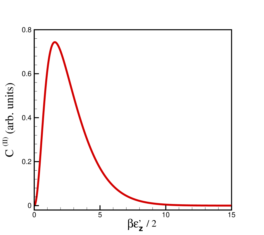
Figure 1: Magnetic field (thermal) variation of the $C^{(II)}$.

IV.1 Discussion on the field dependence of the Heat Capacity

In this section, we have studied the magnetic field dependence of the Heat capacity of glasses at low temperature. We have assumed that the tunneling particles carry both an angular momentum and a nuclear spin. So, the magnetic field couple to both terms.

We have examined our results numerically for arbitrary angle of EFG and different phases between the quadrupole moments on each well. The final results are not influenced if we only consider the simple case of $\theta=0$ and considering that $\epsilon_{q}^{R}=\epsilon_{q}^{L}=\epsilon_{q}$. Thus, we have reported our results in the mentioned special case where we can find an analytical expression for the specific heat behaviour. In this respect, the total partition function of system can be splitted into the multiplication of three separate terms. Therefore, the Heat capacity is composed of three terms, the TLS contribution ($C_{TLS}$), the nuclear ($C^{(I)}$) and the angular momentum ($C^{(II)}$) parts. The magnetic field dependence will arise from $C^{(I)}$ and $C^{(II)}$.

We have introduced the generalized Hamiltonian which takes into account the mentioned degrees of freedom. The direction of external magnetic ($\theta^{\prime},\phi^{\prime}$) field has been considered arbitrary with respect to the EFG direction of each TLS. However, the outcome will be averaged over this spherical angle which can be contracted as a constant to the final results. We have calculated the contribution of $C_{TLS}$ and $C^{(II)}$ exactly while the effect of nuclear spin ($C^{(I)}$) has been treated in a thermal expansion up to the second order corrections.

The different scale of Zeeman energy for the nuclear moment and the angular momentum of the tunneling entity is roughly $\epsilon_{z}/\epsilon_{z}^{\prime}\approx 10^{-3}$. Thus, for low magnetic fields $\beta\epsilon_{z}^{\prime}<10$ the dominant effect comes from the angular momentum part ($C^{(II)}$). Our calculation shows that at low magnetic field this contribution is proportional to the square of magnetic field, $C^{(II)}\simeq B^{2}$ (Eq.(69). However, $C^{(II)}$ reaches a maximum at $\beta\epsilon_{z}^{\prime}\simeq 3$ and then decreases to zero for $\beta\epsilon_{z}^{\prime}>20$ (see Fig.(1)).

For low magnetic field ($B<10T$) our result predict a Schottky like peak in the specific heat of glasses which have nonzero angular momentum for the tunneling entity. Or at least the sample has some impurity with nonzero $J$ (angular momentum). This result is in agreement with the recent experimental observations for Duran, AlBaSi strehlow-web and Suprasil Str04 . The data show explicitly an upward increase of the specific heat versus the magnetic filed for $B<0.5\mbox{T}$ and monotonic decrease for $B>1\mbox{T}$ at $T<1\mbox{K}$.

We have also predicted that for high magnetic fields ($\beta\epsilon_{z}^{\prime}>20$) the dominant contribution to the specific heat comes from the nuclear moments which shows a quadratic dependence on the field (Eq. 68).

In this paper we have studied the special case that the impurities have only the intrinsic angular momentum part. For the general case of impurities (for example electrons) with angular momentum, $J>\frac{1}{2}$ (spin + orbit), we should take into account the effect of spin - orbit interaction. Which means that at zero magnetic field the levels $m^{\prime}=-J,...,J-1,J$ may have different energies due to the crystal field splitting.

However, if we consider $J=0$ which means to have a pure glass without magnetic impurities like BK7 the nuclear quadrupole term is the only dominant term in the specific heat. So, the present calculations predict a quadratic dependence on the magnetic field, and $1/T^{2}$ dependence on temperature. As far as we know there is no experimental result for this case. Therefore it might be a good suggestion for future experiments.

V Summary

Based on the polarization echoes experiments Nag04 we believe that the nuclear quadrupole model should provide the rightful explanation for the intriguing behavior of the dielectric properties of glasses. A relaxation spectrum rather sensitive to the orientation of the nuclear quadrupoles is providing a relaxation susceptibility strongly dependent on the applied magnetic field Dor06 , driving us to the conclusion that the observed magnetic properties of glasses might have a relaxation origin. Other effects like non-linearities with the voltage Bur05 , or cooperative TLS behavior might as well be found contributing.

Appendix A Generalized TLS Hamiltonian with both nuclear spin and angular momentum

The aim of this appendix is to find the generalized TLS Hamiltonian with both nuclear spin and angular momentum. In the similar way leading to the Eq. 34, we can write the total Hamiltonian as:

$$\left(\begin{array}[]{cc}H^{L}+\frac{\Delta}{2}\cdot\textbf{1 }&\frac{\Delta_{0}}{2}\cdot\textbf{1 }\\ \frac{\Delta_{0}}{2}\cdot\textbf{1 }&H^{R}-\frac{\Delta}{2}\cdot\textbf{1 }\end{array}\right)\vspace{0.5cm}$$ (73)

where 1 is the unit matrix of rank $(2I+1)\times(2J+1)$. $H^{L}=V_{Q}^{L}+H_{Z}^{L}$ and $H^{R}=V_{Q}^{R}+H_{Z}^{R}$ are defined for particles in the left and right wells, respectively. The state in each well (L or R) can be characterized by $\mid\psi^{L(R)}_{[I,m],[J,m^{\prime}]}\rangle=\mid L(R)\rangle\bigotimes\mid I,m\rangle\bigotimes\mid J,m^{\prime}\rangle$ and consequently the matrix element of the Hamiltonian is defined by the following equation,

$$H^{L(R)}_{mm^{\prime},nn^{\prime}}=\langle\psi^{L(R)}_{[I,m],[J,m^{\prime}]}\mid H^{L(R)}\mid\psi^{L(R)}_{[I,n],[J,n^{\prime}]}\rangle.$$ (74)

After some simple algebra we can easily show that for $H^{R}_{mm^{\prime},nn^{\prime}}$ we obtain

$$H^{R}_{mm^{\prime},nn^{\prime}} = \left\{\epsilon_{q}^{R}\left[\Upsilon_{m,m-2}e^{2i\theta}\delta_{m-2,n}+\Upsilon_{m,m+2}e^{-2i\theta}\delta_{m+2,n}\right]-\epsilon_{z}\sin\theta^{{}^{\prime}}\left[e^{i\phi^{{}^{\prime}}}\alpha_{-}^{m}\delta_{m+1,n}+e^{-i\phi^{{}^{\prime}}}\alpha_{+}^{m}\delta_{m-1,n}\right]\right.$$ (75)

$$+ \left.\left[-m^{\prime}\epsilon_{z}^{\prime}-\epsilon_{z}\cos\theta^{{}^{\prime}}m+\epsilon_{q}^{R}\Upsilon_{m,m}\right]\delta_{m,n}\right\}\delta_{m^{\prime},n^{\prime}}.$$

where $\theta^{{}^{\prime}}$ and $\phi^{{}^{\prime}}$ define the direction of magnetic field in the basis $(e_{1},e_{2},e_{3})$; $\alpha_{\pm}^{m}$ and $\Upsilon_{m,m^{\prime}}$ are given by Eqs. (37 & 38) . In a similar manner we can obtain the matrix element of the Hamiltonian for the particles in the left well $H^{L}_{m,n}$ by taking $\theta=0$ and changing $\epsilon_{q}^{R}\longmapsto\epsilon_{q}^{L}$ in the above equation.

References

• (1) P. Esquinazi (ed.), Tunneling Systems in Amorphous and Crystalline Solids, Springer Berlin Heidelberg, New York (1998).
• (2) R. C. Zeller and R. O. Pohl, Phys. Rev. B 4, 2029 (1971).
• (3) N. Ahmad, K. W. Hutt, and W. A. Phillips, J. Phys. C 19, 3765 (1986).
• (4) W. A. Philips, J. Low. Temp. Phys. 7, 351 (1972).
• (5) P. W. Anderson, B. I. Halperin and C. M. Varma, Philos. Mag. 25, 1 (1972).
• (6) P.Β Strehlow, C.Β Enss, S. Hunklinger, Phys.Β Rev.Β Lett. 80, 5361 (1998).
• (7) P.Β Strehlow et al., Phys.Β Rev.Β Lett. 84, 1938 (2000).
• (8) M.Β Wohlfahrt et al., Europhys.Β Lett. 56, 690 (2001)
• (9) J. Le Cochec, F.Β Ladieu, P.Β Pari, Phys.Β Rev.Β B 66, 064203 (2002).
• (10) R. Haueisen and G. Weiss, Physica B 316, 555 (2004).
• (11) S. Ludwig, C. Enss, P. Strehlow, and S. Hunklinger, Phys.Β Rev.Β Lett. 88, 075501 (2002).
• (12) C.Β Enss and S. Ludwig, Phys.Β Rev.Β Lett. 89, 075501 (2002).
• (13) S. Hunklinger and C. Enss, Insulating and Semiconducting Glasses, World Scientific, Hong Kong (2000).
• (14) A. WΓΌrger, From coherent Tunnelling to Relaxation, Springer Tracts in Modern Physics, 135, Springer, Berlin, Heidelberg, New York (1997).
• (15) S.Β Kettemann, P. Fulde, and P. Strehlow, Phys.Β Rev.Β Lett. 83, 4325 (1999).
• (16) V. Lubchenko and P. Wolynes, Phys. Rev. Lett. 87, 195901 (2001).
• (17) A. Langari, Phys. Rev. B 65, 104201 (2002).
• (18) A. Akbari and A. Langari, Phys. Rev. B, 72, 024203 (2005).
• (19) A.Β WΓΌrger, Phys.Β Rev.Β Lett. 88, 077502 (2002).
• (20) A.Β WΓΌrger, A. Fleischmann, C.Β Enss, Phys.Β Rev.Β Lett. 89, 237601 (2002).
• (21) A. WΓΌrger, J. Low Temp. Phys. 137, 143 (2004).
• (22) P. Nagel, A. Fleishmann, S. Hunklinger and C. Enss, Phys. Rev. Lett. 92, 245511 (2004).
• (23) D. Bodea and A. WΓΌrger, J. Low Temp. Phys. 136, 39 (2004).
• (24) D. Bodea and A. WΓΌrger, to be published.
• (25) I. Y. Polishchuk et al., J. Low Temp. Phys. 140, 355 (2005).
• (26) M. Meissner and P. Strehlow, J. Low Temp. Phys. 137, 355 (2004).
• (27) A. Abragam, The Principles of Nuclear Magnetism, Oxford University Press (1989).
• (28) A. Akbari and A. Langari, Preprint.
• (29) J. JΓ€ckle, Z. Phys. 257, 212 (1972).
• (30) A. Burin, private communication.
• (31) The data can be found in the following URL, (http://www.hmi.de/bensc/sample-env/index_en.html)