Small cosmological constant in seesaw mechanism with breaking down SUSY

Abstract

The observed small value of cosmological constant can be naturally related with the scale of breaking down supersymmetry in agreement with other evaluations in particle physics.

I Introduction

Recent precise observations in cosmology snIa ; deceldata ; SNLS ; wmap ; baryon prefer for the model of flat Universe, which has the energy density composed by following three dominant components: baryons, dark matter and dark energy with fractions of energy approximately given by $\Omega_{\rm b}\approx 0.04$, $\Omega_{\rm dm}\approx 0.21$ and $\Omega_{\rm de}\approx 0.75$, respectively. The dark energy is dynamically fitted by a quintessence quint , that is a slowly evolving scalar-field, whose potential energy imitates the cosmological constant. The introduction of quintessence seems to be reasonable, since the cosmological constant itself Weinberg-RMP should give the energy density

$$\rho_{\Lambda}=\mu_{\Lambda}^{4},\quad\mbox{at}\quad\mu_{\Lambda}\approx 0.25\cdot 10^{-11}\;\mbox{GeV,}$$ (1)

which leads to the artificially small scale in particle physics. The quintessence serves to produce such the scale due to the evolution of potential energy from natural values to the present-day point.

There is an alternative way to show that the small value of $\mu_{\Lambda}$ is not artificial but natural. Indeed, fluctuations between two vacuum-states with exact and broken down supersymmetry can result in small mixing and appearance of stationary vacuum level with the small cosmological constant. Thus, the cosmological constant could indicate the scale of supersymmetry breaking.

In Section II of present paper we assign the cosmological constant to the energy density of vacuum (zero-point) modes. If supersymmetry (SUSY) is exact the vacuum is flat, while breaking down SUSY results in a negative density of energy determined by the scale of SUSY breaking $\mu_{\mbox{\footnotesize{x}}}$, and the vacuum state is given by Anti-de Siter spacetime (AdS). We argue for the two vacua correlate. The decay of flat vacuum to AdS one false-decay is forbidden due to the gravity effects CdL , introducing a critical density of AdS state unreachable in supergravity Wein-S . Therefore, two vacuum-levels can get mixing, not the decay.

In Section III we consider static spherically-symmetric action of gravity and scalar field interpolating between two its positions in minima of potential with zero and negative values of energy density. Such the configuration describes the bubble of AdS vacuum separated from the flat vacuum by the domain wall. We show that the domain wall does not propagate to infinity. Contrary, it has a finite size. We compare the situation with the case of gravity switched off as well as with the calculation of static energy describing the decay of flat vacuum if not forbidden. We estimate the size of bubble fluctuations, responsible for the mixing.

The mixing of two stationary vacuum-levels is studied in Section IV in cases of both thin and thick domain walls. The suppression of mixing matrix element leads to seesaw mechanism with small mixing angle Fritzsch , so that the observed small value of cosmological constant is naturally derived in terms of SUSY breaking scale $\mu_{\mbox{\footnotesize{x}}}$ and Planck mass.

The estimates in Section V show that thin domain walls correspond to low scale of SUSY breaking about $\mu_{\mbox{\footnotesize{x}}}\sim 10^{4}$ GeV, while thick domain walls give high scales of the order of $\mu_{\mbox{\footnotesize{x}}}\sim 10^{12-13}$ GeV.

In Section VI we formulate a model of superpotential, which allows us to demonstrate that thin domain walls correspond to gauge-mediated SUSY breaking as well as thick domain walls do to gravity-mediated SUSY breaking. Then, we evaluate the mixing angle in Section VII.

A connection of vacuum superposition to the problem of generations in the Standard Model (SM) of particle interactions is discussed in Section VIII, wherein we qualitatively map the way for the origin of three generations.

In Conclusion we summarize our results and focus on some further questions.

II Vacuum modes and cosmological constant

The quantization of free bosonic and fermionic fields give hamiltonians in terms of creation and annihilation operators

$$\begin{array}[]{l}E_{\mbox{\footnotesize{b}}}\hskip-3.0pt={\displaystyle\hskip-3.0pt\int\hskip-3.0pt\frac{{\rm d}^{3}\boldsymbol{k}}{(2\pi)^{3}}}\,\frac{1}{2}\big{\{}\mathfrak{a}^{\dagger}_{\mbox{\footnotesize{b}}}(\boldsymbol{k})\mathfrak{a}_{\mbox{\footnotesize{b}}}(\boldsymbol{k})+\mathfrak{a}_{\mbox{\footnotesize{b}}}(\boldsymbol{k})\mathfrak{a}^{\dagger}_{\mbox{\footnotesize{b}}}(\boldsymbol{k})\big{\}}\,\omega_{\mbox{\footnotesize{b}}}(\boldsymbol{k}),\\[14.22636pt] E_{\mbox{\footnotesize{f}}}\hskip-3.0pt={\displaystyle\hskip-3.0pt\int\hskip-3.0pt\frac{{\rm d}^{3}\boldsymbol{k}}{(2\pi)^{3}}}\,\frac{1}{2}\big{\{}\mathfrak{a}^{\dagger}_{\mbox{\footnotesize{f}}}(\boldsymbol{k})\mathfrak{a}_{\mbox{\footnotesize{f}}}(\boldsymbol{k})-\mathfrak{a}_{\mbox{\footnotesize{f}}}(\boldsymbol{k})\mathfrak{a}^{\dagger}_{\mbox{\footnotesize{f}}}(\boldsymbol{k})\big{\}}\,\omega_{\mbox{\footnotesize{f}}}(\boldsymbol{k}),\end{array}$$ (2)

respectively, for each mode with $\omega(\boldsymbol{k})=\sqrt{m^{2}+\boldsymbol{k}^{2}}$.

The commutation and anti-commutation relations for bosons and fermions

$$[\mathfrak{a}_{\mbox{\footnotesize{b}}}(\boldsymbol{k}),\mathfrak{a}^{\dagger}_{\mbox{\footnotesize{b}}}(\boldsymbol{k}^{\prime})]=\{\mathfrak{a}_{\mbox{\footnotesize{f}}}(\boldsymbol{k}),\mathfrak{a}^{\dagger}_{\mbox{\footnotesize{f}}}(\boldsymbol{k}^{\prime})\}=(2\pi)^{3}\delta(\boldsymbol{k}-\boldsymbol{k}^{\prime}),$$ (3)

involve the delta-function at zero if $\boldsymbol{k}=\boldsymbol{k}^{\prime}$. It is related with the spatial volume

$$(2\pi)^{3}\delta(\boldsymbol{k})\Big{|}_{\boldsymbol{k}=0}=\int{\rm d}^{3}\boldsymbol{r}\cdot{\rm e}^{{\rm i}\boldsymbol{r}\cdot\boldsymbol{k}}\Big{|}_{\boldsymbol{k}=0}=\mbox{\small{Volume}.}$$

Then, the energy of single field-mode is given by the expression

$$E=\hskip-3.0pt\int\frac{{\rm d}^{3}\boldsymbol{k}}{(2\pi)^{3}}\,\mathfrak{a}^{\dagger}(\boldsymbol{k})\mathfrak{a}(\boldsymbol{k})\cdot\omega(\boldsymbol{k})+(-1)^{F}\hat{\rho}\cdot\mbox{\small{Volume}},$$ (4)

where $F=\{0,1\}$ denotes the fermion number for bosonic or fermionic mode, correspondingly, while the energy density of zero-point mode $\hat{\rho}$ equals

$$\hat{\rho}=\frac{1}{2}\int\frac{{\rm d}^{3}\boldsymbol{k}}{(2\pi)^{3}}\;\omega(\boldsymbol{k}).$$ (5)

The vacuum energy has the density

$$\rho=\sum\limits_{\mbox{\tiny modes}}(-1)^{F}\hat{\rho}.$$ (6)

At $\omega>0$, the exact supersymmetry guarantees the followings:

• The number of bosonic modes is equal to the number of fermionic ones

  $$I_{W}=\sum\limits_{\mbox{\tiny modes}}(-1)^{F}=0.$$

• Masses of superpartners are equal to each other

  $$m_{\mbox{\footnotesize{b}}}=m_{\mbox{\footnotesize{f}}},\quad\Rightarrow\quad\omega_{\mbox{\footnotesize{b}}}(\boldsymbol{k})=\omega_{\mbox{\footnotesize{f}}}(\boldsymbol{k}).$$

Therefore, the supersymmetric vacuum state $|\Phi_{\mbox{\footnotesize{s}}}\rangle$ has zero energy density $\rho_{\mbox{\footnotesize{s}}}=0$ due to the contribution by the vacuum zero-point modes. The Witten’s index $I_{W}$ Witten_index counting for all physical modes would differ from zero in the supersymmetric theory Weinberg-VIII , if one introduces different numbers of bosonic and fermionic modes with zero energy $\omega=0$, but such the situation would correspond to the case, when, due to the conservation law for the number of unpaired zero-energy modes, the supersymmetry cannot be spontaneously broken in evident contradiction with observations.

A loss of balance between the modes produces a non-zero cosmological constant. The balance could be lost because of essential deviations from dispersion laws of free particles, that can appear due to a strong field dynamics beyond the asymptotically free region. Then, SUSY is broken down.

In ordinary schemes the SUSY breaking down is described by generation of different masses for superpartners at scales below $\mu_{\mbox{\footnotesize{x}}}$, the characteristic energy of SUSY breaking. For instance, in the gauge-mediated scenario of SUSY breaking the superpartners of fields in the SM acquire masses of the order

$$m\sim\frac{\alpha_{g}}{4\pi}\,\mu_{\mbox{\footnotesize{x}}}\ll\mu_{\mbox{\footnotesize{x}}},$$

while the number of modes in the matter sector of theory is preserved, and the masses satisfy a rule of splitting

$$\sum\limits_{\mbox{\tiny matter modes}}\hskip-11.38109pt(-1)^{F}=0,\qquad\sum\limits_{\mbox{\tiny matter modes}}\hskip-11.38109pt(-1)^{F}m^{2}=0.$$ (7)

Effectively at scales below $\mu_{\mbox{\footnotesize{x}}}$ we put the dispersion law $\omega(\boldsymbol{k})=\sqrt{\boldsymbol{k}^{2}+m^{2}}$. SUSY is restored at scales higher than $\mu_{\mbox{\footnotesize{x}}}$. Then, the integration in the energy density of single vacuum-mode is actually cut off by $\mu_{\mbox{\footnotesize{x}}}$ because of exact cancelling by the superpartner contribution, and we easily get

$$\begin{array}[]{rl}\hat{\rho}=&\displaystyle\frac{1}{2}\int\limits_{0}^{\mu_{\mbox{\footnotesize{x}}}}\frac{k^{2}{\rm d}k}{(2\pi)^{3}}\;\sqrt{k^{2}+m^{2}}\int{\rm d}\Omega\\[17.07164pt] =&\displaystyle\frac{2}{(16\pi)^{2}}\;m^{4}\,(\sinh 4y-4y),\end{array}$$ (8)

where

$$y=\mbox{arcsinh}\frac{\mu_{\mbox{\footnotesize{x}}}}{m}=\ln\left(\frac{\mu_{\mbox{\footnotesize{x}}}}{m}+\sqrt{\frac{\mu_{\mbox{\footnotesize{x}}}^{2}}{m^{2}}+1}\;\right).$$

At $\frac{\mu_{\mbox{\footnotesize{x}}}}{m}\gg 1$ the leading contribution to the vacuum energy in the observable matter sector is about

$$\sum\limits_{\mbox{\tiny matter modes}}\hskip-11.38109pt(-1)^{F}\hat{\rho}\sim-\hskip-14.22636pt\sum\limits_{\mbox{\tiny matter modes}}\hskip-11.38109pt(-1)^{F}m^{4}\ln\frac{\mu_{\mbox{\footnotesize{x}}}}{m},$$ (9)

since terms of the form $\mu_{\mbox{\footnotesize{x}}}^{4}$ are cancelled due to the balance between the superpartner modes, i.e. Witten’s index is equal to zero, while terms of the form $m^{2}\mu_{\mbox{\footnotesize{x}}}^{2}$ nullify due to the sum rule for the mass splitting (7). The supercharge relation with the hamiltonian ensures the positivity of matter contribution to the vacuum energy (9), i.e. up to fine effects in higher orders of small ratio $m/\mu_{\mbox{\footnotesize{x}}}$ one should expect the following sum rule

$$\sum\limits_{\mbox{\tiny matter modes}}\hskip-11.38109pt(-1)^{F}m^{4}\ln\frac{\mu_{\mbox{\footnotesize{x}}}}{m}<0.$$

However, the direct breaking down SUSY at tree level in the minimal extension of SM contradicts with observations, since the mass sum rules (7) introduce too light superpartners for the particles of observable sector Weinberg-VIII . So, SUSY is broken in a hidden sector, which can carry zero or nonzero quantum numbers of SM, and the particles of observable sector acquire masses due to loops with particles from the hidden sector, that plays the role of messenger. The first scenario with messengers carrying nonzero SM charges refers to the gauge-mediated SUSY breaking, while the second possibility of sterile messengers does to gravity-mediated one. The masses of messengers are of the order of SUSY breaking scale, $m\sim\mu_{\mbox{\footnotesize{x}}}$. Hence, the contribution of hidden sector to the density of vacuum energy is dominant, $\rho\sim\pm\mu_{\mbox{\footnotesize{x}}}^{4}$. The sign can be certainly fixed, if one takes into account the result by W. Nahm, who algebraically found Nahm , that SUSY realization is forbidden in four-dimensional (4D) spacetime with a positive density of vacuum energy, while it is permitted in 4D spacetime with a negative density of vacuum energy.

In the gravity sector, the SUSY breaking leads to two massless modes of graviton with spirality $\pm 2$ as well as to two massive modes of graviton superpartner, the gravitino with spirality $\pm\frac{3}{2}$, while in addition the goldstino with spirality $\pm\frac{1}{2}$ becomes massive and it complements higher spirality modes of gravitino to the full set $\{\pm\frac{3}{2},\pm\frac{1}{2}\}$. Therefore, the goldstino breaks the balance between the number of bosonic and fermionic modes in the gravity sector. Hence, the vacuum energy could gain the large negative contribution of two goldstino-modes

$$\sum\limits_{\mbox{\tiny gravity}}(-1)^{F}\hat{\rho}\sim-\hskip-5.69054pt\sum\limits_{\mbox{\tiny goldstino}}\hskip-5.69054pt\hat{\rho}\sim-\frac{1}{8\pi^{2}}\,\mu_{\mbox{\footnotesize{x}}}^{4}.$$ (10)

However, the goldstino is a composition of hidden sector spinor fields, i.e. its two modes are superpartners for the bosonic modes from the non-gravity sector. Therefore, the true value of vacuum energy is determined by the whole hidden sector as it has been matched above.

Thus, the vacuum modes in supergravity with SUSY broken below $\mu_{\mbox{\footnotesize{x}}}$ give the negative cosmological term, that corresponds to Anti-de Sitter spacetime. We denote such the state by $|\Phi_{\mbox{\footnotesize{x}}}\rangle$, which has got the negative energy density $\rho=-\rho_{\mbox{\footnotesize{x}}}\sim-\mu_{\mbox{\footnotesize{x}}}^{4}$.

Such the nature of vacuum energy assumes that two states $|\Phi_{\mbox{\footnotesize{s}}}\rangle$ and $|\Phi_{\mbox{\footnotesize{x}}}\rangle$ correlate, i.e. they are not completely independent, since the vacuum modes with momenta greater $\mu_{\mbox{\footnotesize{x}}}$ are common for both states. In other words, we can introduce the correlation length determined by the scale of SUSY beraking $\lambda_{\mbox{\footnotesize{x}}}=1/\mu_{\mbox{\footnotesize{x}}}$, so that dynamical processes at characteristic distances less than $\lambda_{\mbox{\footnotesize{x}}}$ involve the correlation of two vacuum-states with zero and negative cosmological constants. The transitions between two states can have a status of whether we get the decay of unstable state into the stable one or mixing that leads to two stationary levels. The overlapping of two vacua is associated with the domain wall separating the bubble of lower-energy AdS-vacuum from the exterior of higher-energy flat vacuum. The process of decay is described in terms of bounce, the solution of 4D Euclidean spherically symmetric field-equations for a scalar field interpolating between local minima of its potential in the region of domain wall. The bounce determines the quasiclassical exponent of penetration between two levels of vacuum. Coleman and De Luccia CdL shown that the bounce is essentially modified by gravity that introduces a critical surface tension of domain wall, while S.Weinberg Wein-S found that the real surface density of energy exceeds the critical one in supergravity. Thus, the decay does not take place. Therefore, we focus on stationary 3D spherically symmetric fluctuations of scalar field, that provide the mixing of two vacuum-states, if such the domain wall cannot evolve to spatial infinity.

III Static energy and domain wall

For fields independent of time, the action is converted to the static potential $U^{\rm stat}$ multiplied by the factor of total time

$$S=\int\mathscr{L}\,\sqrt{-g}\;\;{\mathrm{d}}^{4}x\;\mapsto\;S^{\rm stat}=-U^{\rm stat}\int{\mathrm{d}}t,$$ (11)

since the metric could be also written in the static form, too. In the case of spherical symmetry we get the metric

$${\mathrm{d}}s^{2}=\widetilde{\mathtt{B}}(r)\,{\mathrm{d}}t^{2}-\frac{1}{\mathtt{B}(r)}\,{\mathrm{d}}r^{2}-r^{2}({\mathrm{d}}\vartheta^{2}-\sin^{2}\vartheta\,{\mathrm{d}}\varphi^{2}),$$ (12)

so that $\sqrt{-g}=r^{2}\sin\vartheta\,\sqrt{\widetilde{\mathtt{B}}/\mathtt{B}}$, while in the lagrangian of real scalar field $\phi(r)$ dependent of the radius

$$\mathscr{L}_{f}=\frac{1}{2}\,g^{\mu\nu}\partial_{\mu}\phi\partial_{\nu}\phi-V(\phi),$$

the gradient term survives in the form

$$g^{\mu\nu}\partial_{\mu}\phi\partial_{\nu}\phi\;\mapsto\;-(\phi^{\prime})^{2}\,\mathtt{B},$$ (13)

where the prime denotes the derivative with respect to the distance $r$. Then the field equation reads as follows

$$\phi^{\prime\prime}+u^{\prime}\phi^{\prime}+\frac{2}{r}\,\phi^{\prime}=\frac{1}{\mathtt{B}}\;\frac{\partial V}{\partial\phi}$$ (14)

with $u=\frac{1}{2}\ln(\widetilde{\mathtt{B}}\mathtt{B})$. The field equation allows the treatment in terms of Newtonian mechanics by the assignment of $\phi^{\prime\prime}$ to the “acceleration” of “coordinate” $\phi$, so that the force contains the “potential term” $\partial V/\partial\phi$ with “external parameter” $\mathtt{B}$ and the “friction” proportional to the “velocity” $\phi^{\prime}$. The friction coefficient $2/r$ enters because of the spatial dimension equal to 3, while the gravitation results in the friction if $u^{\prime}$ is positive, otherwise the gravitation causes the enlarging the acceleration.

The energy-momentum tensor $T_{\mu\nu}=\partial_{\mu}\phi\partial_{\nu}\phi-g_{\mu\nu}\mathscr{L}_{f}$ is composed by diagonal elements

$$\begin{array}[]{rcl}T_{t}^{t}&=&+\frac{1}{2}\,(\phi^{\prime})^{2}\,\mathtt{B}+V,\\[5.69054pt] T_{r}^{r}&=&-\frac{1}{2}\,(\phi^{\prime})^{2}\,\mathtt{B}+V,\end{array}$$ (15)

and $T_{\vartheta}^{\vartheta}=T_{\varphi}^{\varphi}=T_{t}^{t}$, which enter the Einstein equation

$$R_{\mu\nu}-\frac{1}{2}\,g_{\mu\nu}R=8\pi G\,T_{\mu\nu}.$$

Hence, due to the relation of scalar curvature with the trace of energy-momentum tensor

$$R=-8\pi G\,T,$$

the lagrangian of general relativity equal to

$$\mathscr{L}_{GR}=-\frac{R}{16\pi\,G},$$

and the static field lagrangian equal to

$$\mathscr{L}_{f}=-T_{t}^{t},$$

we get the stationary energy depending on the size of sphere $r_{A}$ inside of which the matter has a non-zero energy,

$$U^{\rm stat}(r_{A})=-4\pi\int\limits_{0}^{r_{A}}V(\phi)\,\sqrt{\frac{\widetilde{\mathtt{B}}}{\mathtt{B}}}\;r^{2}\,{\mathrm{d}}r.$$ (16)

The static potential equals zero if the scalar field is global, and it positioned at a local minimum of its potential with $V=0$. If the local minimum at constant field is positioned at negative $V=-\rho_{\mbox{\footnotesize{x}}}$, then we arrive to Anti-de Sitter spacetime with

$$\widetilde{\mathtt{B}}_{\rm AdS}=\mathtt{B}_{\rm AdS}=1+\frac{r^{2}}{\ell^{2}},\qquad\frac{1}{\ell^{2}}=\frac{8\pi\,G}{3}\,\rho_{\mbox{\footnotesize{x}}},$$ (17)

and the positive static potential

$$U^{\rm stat}_{{\rm AdS}}=\frac{4\pi}{3}\,r_{A}^{3}\,\rho_{\mbox{\footnotesize{x}}}.$$ (18)

Let $\phi(r)$ be the solution, which interpolates between two local minima of potential with zero energy and negative $V=-\rho_{\mbox{\footnotesize{x}}}$. To the moment, we restrict ourselves by the consideration of thin domain wall, so that the field is essentially changing in a narrow layer of width $\delta r$ near the sphere of radius $r_{A}$ and $\delta r\ll r_{A}$. Then, the stationary potential is composed of two summands with integration in limits $[0,r_{A}]$ and $[r_{A},r_{A}+\delta r]$ respectively,

$$U^{\rm stat}(r_{A})=\frac{4\pi}{3}\,r_{A}^{3}\,\rho_{\mbox{\footnotesize{x}}}-4\pi\,r_{A}^{2}\,W_{A},$$ (19)

where $W_{A}$ determines the surface energy per unit area

$$W_{A}(r_{A})=\frac{1}{r_{A}^{2}}\int\limits_{r_{A}}^{r_{A}+\delta r}V(\phi)\,\sqrt{\frac{\widetilde{\mathtt{B}}}{\mathtt{B}}}\;r^{2}\,{\mathrm{d}}r,$$ (20)

and it is positive if the local minima are separated by sufficiently high potential barrier.

At $\delta r\ll r_{A}\ll\ell$ we can safely neglect the contribution of friction in the field equation (14), since by the order of magnitude $\phi^{\prime\prime}\sim\delta\phi/(\delta r)^{2}$, while the spatial term is at the level of $\phi^{\prime}/r\sim\delta\phi/(\delta r)^{2}\cdot\delta r/r_{A}\ll\phi^{\prime\prime}$, and the metric elements $\widetilde{\mathtt{B}}$, $\mathtt{B}$ are infinitely close to unit, so that $u^{\prime}\phi^{\prime}\sim r_{A}^{2}/\ell^{2}\cdot 1/\delta r\cdot\delta\phi/\delta r\ll\phi^{\prime\prime}$. Therefore, in this limit the field equation does not involve any scale parameter external with respect to the potential $V$, and it reproduces the “kink” solution with the small value of $r_{A}$ and the width $\delta r$ determined by a mass parameter in $V$, since the field equation yields $1/(\delta r)^{2}\sim\delta V/(\delta\phi)^{2}\sim\partial^{2}V/\partial\phi^{2}$. Note, that the gradient contribution to the energy density $T_{t}^{t}$ equals the potential term CdL . The kink sets the distribution of matter determining the behavior of metric. Thus, the thin domain wall can be established in the limit of small bubble.

At $\delta r\ll r_{A}\sim\ell$ the gravitational contribution to the field equation has two regimes. At the inner surface of domain wall, i.e. at the edge of AdS spacetime, the metric elements $\widetilde{\mathtt{B}}$, $\mathtt{B}$ are about unit and $u^{\prime}>0$ at $u^{\prime}\sim r_{A}/\ell^{2}\sim 1/r_{A}$, so that one could neglect its contribution as well as the friction term. Inside the wall the metric elements $\widetilde{\mathtt{B}}$, $\mathtt{B}$ can rapidly fall to unit and $u^{\prime}<0$ at $u^{\prime}\sim 1/\delta r$, so that $u^{\prime}\phi^{\prime}\sim\phi^{\prime\prime}$ and the gravity term accelerates the evolution of field from the negative minimum to positive one, if the field evolves from a small value to larger one. Therefore, the surface tension $W_{A}$ can depend on the bubble size, but the width of the domain wall still remains at the same order as it was at small $r_{A}$, that preserves the magnitude of $W_{A}$, too. In this region of bubble size the gradient term in the energy density is comparable to the potential.

We can evaluate the surface tension $W_{A}$ by setting $\widetilde{\mathtt{B}}\sim\mathtt{B}$ and $V\sim(\phi^{\prime})^{2}$, so that $W_{A}\sim\int\sqrt{V}\phi^{\prime}{\rm d}r\sim\int\sqrt{V}{\rm d}\phi$, while in the supersymmetric theory with the chiral superfield the potential is determined by the superpotential $f$ as $V=|\partial f/\partial\phi|^{2}$, hence, $W_{A}\sim|f_{0}|$, where $f_{0}$ is the superpotential value at the vacuum. In supergravity the negative vacuum energy at the extremal of superpotential is assigned to the superpotential itself in the linear order in Newtonian constant $G$

$$\rho_{\mbox{\footnotesize{x}}}=24\pi G\,|f_{0}|^{2},$$ (21)

that yields

$$W_{A}\sim m_{\mathtt{Pl}}\,\mu_{\mbox{\footnotesize{x}}}^{2},$$ (22)

where $m_{\mathtt{Pl}}=1/\sqrt{G}\sim 10^{19}$ GeV is the Planck mass.

At $r_{A}\gg\ell$ the metric elements at the edge of AdS spacetime become large $\widetilde{\mathtt{B}}\sim\mathtt{B}\sim r_{A}^{2}/\ell^{2}\gg 1$, and the gravity term in the left hand side of field equation (14) can still be essential, since at $\delta u\sim 1$ we estimate $u^{\prime}\phi^{\prime}\sim\delta\phi/(\delta r)^{2}\sim\phi^{\prime\prime}$, while condition $\mathtt{B}\gg 1$ leads to suppression of gradient term in the energy as well as to more thick domain wall because of the approximation $\mathtt{B}\cdot\phi^{\prime\prime}\sim\partial V/\partial\phi$, hence, $(\phi^{\prime})^{2}\ll V$ and $1/(\delta r)^{2}\sim\partial^{2}V/\partial\phi^{2}\cdot\ell^{2}/r_{A}^{2}$. Note, that the width of domain wall essentially exceeds its “natural” value $\delta r_{0}$ determined by the parameters of potential $V$ at small $r_{A}$, and it linearly grows with $r_{A}$ like $\delta r\sim\delta r_{0}\cdot r_{A}/\ell$. Switching the regimes in $W_{A}$ versus $r_{A}$ depends on the parameters of potential. The simple example with $W_{A}=W_{A}^{0}\left[1+\frac{r_{A}}{b\ell}\left(1+\tanh\left\{\frac{r_{A}}{b\ell}-b^{\prime}\right\}\right)\right]$ at $b^{\prime}\gg 1$ allows us to draw a conclusion on the critical behavior of $W_{A}$ versus the scale of switch $r_{A}\sim bb^{\prime}\ell$, as it is depicted in Fig. 1, that shows the static potential $U^{\rm stat}$. Moreover, at large $r_{A}\gg\ell$ the domain wall could disintegrate at all.

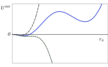
Figure 1: The static potential of bubble with the domain wall versus the bubble radius at different behavior of surface tension: naively constant $W_{A}^{0}$ (long-dashed curve), with a large scale of switching the regime (solid curve) and a low scale of switching (dotted curve). The low scale of switching is not realistic, since it should mean the opportunity of domain-wall motion to infinity, i.e. the decay, that is forbidden (see text).

We assume that the critical scale is large enough in order to provide the materialization of bubble with zero static potential. Then, the bubble can arise in the vacuum with zero density of energy. The characteristic size of such the bubble is given by solving $U^{\rm stat}=0$, that gives

$$r_{A}=\frac{3W_{A}}{\rho_{\mbox{\footnotesize{x}}}}\sim\ell.$$ (23)

The materialization of bubble in the flat vacuum results in the instability, since it takes place at the size of $r_{A}$, that is not positioned at the local minimum of static potential: the domain wall begins to move to the bubble center (see Fig. 1). Furthermore, the zero size of bubble is also unstable: the flat vacuum suffers from fluctuations due to the bubbles of AdS vacuum.

This situation is opposite to the case of switching off the gravity. Indeed, the elimination of gravitational action results in the static potential of bubble

$$U_{0}^{\rm stat}=-\frac{4\pi}{3}r_{A}^{3}\rho_{\mbox{\footnotesize{x}}}+4\pi r_{A}^{2}\widetilde{W}_{A},$$

where

$$\widetilde{W}_{A}(r_{A})=\frac{1}{r_{A}^{2}}\int\limits_{r_{A}}^{r_{A}+\delta r}\left\{V(\phi)+\frac{1}{2}\,(\phi^{\prime})^{2}\right\}\;r^{2}\,{\mathrm{d}}r.$$

This static potential formally has the opposite sign in comparison with (19). Therefore, the domain wall can materialize after the penetration through the potential barrier, but it will move to spatial infinity, that means the decay of flat vacuum to the AdS one. The description of penetration in the presence of gravity was considered by Coleman and De Luccia CdL , involving the Euclidean action and spherical symmetry. So, the critical surface tension was found, and in fact Wein-S the decay is forbidden, since the tension exceeds the critical value.

Indeed, at weak gravitational field, i.e. at $G\to 0$, one can easily evaluate the static energy $E^{\rm stat}$ by summing up

• the energy of AdS-vacuum bubble

  $$M_{\rm b}=-\frac{4}{3}\,\pi r_{A}^{3}\rho_{\mbox{\footnotesize{x}}},$$

• the energy of domain wall $M_{\rm dw}=4\pi r_{A}^{2}\widetilde{W}_{A}$,

• the gravitational potential of wall-bubble interaction

  $$\varphi_{\rm AdS}\,M_{\rm dw}=\varphi_{\rm AdS}\,4\pi r_{A}^{2}\widetilde{W}_{A}=\frac{16}{3}\,\pi^{2}\,G\,r_{A}^{2}\rho_{\mbox{\footnotesize{x}}}\widetilde{W}_{A},$$

• the gravitation of thin domain wall itself

  $$\int\varphi_{\rm dw}{\rm d}M_{\rm dw}=-\frac{G}{r_{A}}\int M_{\rm dw}\,{\rm d}M_{\rm dw}=-8\pi^{2}\,G\,r_{A}^{4}\widetilde{W}_{A}^{2},$$

that yields

$$E^{\rm stat}\approx-\frac{4\pi}{3}\,r_{A}^{3}\rho_{\mbox{\footnotesize{x}}}+4\pi r_{A}^{2}\widetilde{W}_{A}\left(1+\frac{1}{2}\,\frac{r_{A}^{2}}{\ell^{2}}\right)-8\pi^{2}\,G\,r_{A}^{3}\widetilde{W}_{A}^{2}.$$

Beyond the weak-field approximation in Wein-S S.Weinberg found

$$E^{\rm stat}=-\frac{4\pi}{3}\,r_{A}^{3}\rho_{\mbox{\footnotesize{x}}}+4\pi r_{A}^{2}\widetilde{W}_{A}\sqrt{1+\frac{r_{A}^{2}}{\ell^{2}}}-8\pi^{2}\,G\,r_{A}^{3}\widetilde{W}_{A}^{2},$$

where the only modification of wall-bubble term is related with the strict definition of thin domain-wall density of energy in terms of Dirac delta-function

$$\rho_{\rm dw}=\frac{\widetilde{W}_{A}}{\sqrt{\mathtt{B}}}\,\delta(r-r_{A})$$

with $\mathtt{B}=\mathtt{B}_{\rm AdS}$, that preserves the invariance under re-parameterizations of radius. Such the static energy is the mass determining the Schwarzschild metric beyond the bubble and domain wall, so it has nothing with the static value of action, $U^{\rm stat}\neq E^{\rm stat}$. It is the easy task to find that $E^{\rm stat}$ nullifies at

$$r_{A}=\frac{r_{A}^{0}}{1-\left(\frac{r_{A}^{0}}{2\ell}\right)^{2}},\quad\mbox{at}\quad r_{A}^{0}=\frac{3\widetilde{W}_{A}}{\rho_{\mbox{\footnotesize{x}}}}.$$

Therefore, $r_{A}^{0}<2\ell$ and the critical density is given by $\rho_{\mbox{\footnotesize{x}}}^{c}=6\pi\,G\,\widetilde{W}_{A}^{2}$. S.Weinberg shown that the surface tension is constrained by the superpotential as $\widetilde{W}_{A}\geqslant 2|f_{0}|$. Thus, $\rho_{\mbox{\footnotesize{x}}}^{c}>24\pi\,G\,|f_{0}|^{2}=\rho_{\mbox{\footnotesize{x}}}$, and the flat vacuum cannot decay to the AdS one. We have to stress two points. First, the above conclusions on the behavior of $E^{\rm stat}$ is made at exactly constant surface tension $\widetilde{W}_{A}$. Second, at arbitrary $\widetilde{W}_{A}$, nullifying the static energy $E^{\rm stat}$ describes the materialization of bubble, which is strictly considered in CdL in terms of Euclidean 4D-symmetric action, so that one gets the standard quasiclassical calculation of bounce. Contrary, the static action corresponds to unstable fluctuations usually called sphalerons, which are considered in 3D space. Such the bounce and sphaleron are generally different classical solutions, so certainly $E^{\rm stat}\neq U^{\rm stat}$.

As we have just shown the gravity induces the materialization of bubble not propagating to infinity, that means the mixing of two levels, but not the decay.

Thus, due to the unstable bubbles the vacua are not eigenstates of true hamiltonian.

IV Two level system

Consider the quantum system of two stationary vacuum-levels within the domain wall, which is described by the hamiltonian density $\mathscr{H}=H_{\rm vac.}/\mbox{\small{Volume}}$,

$$\begin{array}[]{rl}\mathscr{H}=&-\rho_{\mbox{\footnotesize{x}}}|\Phi_{\mbox{\footnotesize{x}}}\rangle\langle\Phi_{\mbox{\footnotesize{x}}}|+\rho_{\mbox{\footnotesize{s}}}|\Phi_{\mbox{\footnotesize{s}}}\rangle\langle\Phi_{\mbox{\footnotesize{s}}}|\\[8.53581pt] &+\widetilde{\rho}\,\big{\{}|\Phi_{\mbox{\footnotesize{x}}}\rangle\langle\Phi_{\mbox{\footnotesize{s}}}|+|\Phi_{\mbox{\footnotesize{s}}}\rangle\langle\Phi_{\mbox{\footnotesize{x}}}|\big{\}},\end{array}$$ (24)

where $\rho_{\mbox{\footnotesize{x}}}\sim\mu_{\mbox{\footnotesize{x}}}^{4}$ in the AdS vacuum with broken SUSY, while in the supersymmetric vacuum $\rho_{\mbox{\footnotesize{s}}}=0$. We define global complex phases of states, so that the quantity $\widetilde{\rho}$ takes a real positive value. The transition is associated with fluctuations described by the domain wall corresponding to the overlapping region of states. The bubble of AdS vacuum has the size $r_{A}\sim\ell$, the domain wall has a width $\delta r$. Let us, first, evaluate the width of domain wall $\delta r$ in various cases and, second, estimate the mixing matrix element $\widetilde{\rho}=\langle\Phi_{\mbox{\footnotesize{s}}}|\mathscr{H}|\Phi_{\mbox{\footnotesize{x}}}\rangle$.

IV.1 Thin domain wall

If the domain wall is thin, its mass is given by the expression $M_{\rm dw}=4\pi r_{A}^{2}\,W_{A}\sim 4\pi\ell^{2}\delta r\,V_{0}$, where $V_{0}$ is the characteristic height of potential barrier inside the wall. This mass is compensated by the negative mass of bubble $M_{\rm b}=-4\pi r_{A}^{3}\rho_{x}/3\sim-\mu_{\mbox{\footnotesize{x}}}^{4}\ell^{3}$, so that under $\ell\sim m_{\mathtt{Pl}}/\mu_{\mbox{\footnotesize{x}}}^{2}$ we get

$$\delta r\cdot V_{0}\sim\ell\rho_{\mbox{\footnotesize{x}}}\sim m_{\mathtt{Pl}}\,\mu_{\mbox{\footnotesize{x}}}^{2}.$$ (25)

Furthermore, for the chiral superfield, the potential is defined by $V=|\partial f/\partial\phi|^{2}$, where in the linear order in $G$ the superpotential $f_{0}$ at stationary point is related with the negative density of vacuum energy by (21), that gives

$$f_{0}\sim m_{\mathtt{Pl}}\,\mu_{\mbox{\footnotesize{x}}}^{2}\quad\Rightarrow\quad V_{0}\sim\frac{f_{0}^{2}}{(\delta\phi)^{2}}\sim\frac{m_{\mathtt{Pl}}^{2}\,\mu_{\mbox{\footnotesize{x}}}^{4}}{(\delta\phi)^{2}},$$ (26)

where $\delta\phi$ is the characteristic change of field in the domain wall, i.e. the “distance” between two extremal points of the field. Hence, we evaluate the width of domain wall in terms of evolution change of the field,

$$\delta r\sim\frac{(\delta\phi)^{2}}{m_{\mathtt{Pl}}\,\mu_{\mbox{\footnotesize{x}}}^{2}}.$$ (27)

Putting $\delta r\ll r_{A}\sim\ell$, we find

$$\delta\phi\ll m_{\mathtt{Pl}}.$$ (28)

Therefore, the domain wall is thin, if the field dynamics is essentially sub-Planckian.

For instance, we get

$$\delta\phi\sim\mu_{\mbox{\footnotesize{x}}} \Rightarrow \delta r\sim\frac{1}{m_{\mathtt{Pl}}},$$ (29)

$$\delta\phi\sim\sqrt{m_{\mathtt{Pl}}\,\mu_{\mbox{\footnotesize{x}}}} \Rightarrow \delta r\sim\lambda_{\mbox{\footnotesize{x}}}=\frac{1}{\mu_{\mbox{\footnotesize{x}}}}.$$ (30)

The case of $\delta r\sim\lambda_{\mbox{\footnotesize{x}}}$ looks the most natural situation, since the domain wall has the size of correlation length of two vacua. At $\sqrt{m_{\mathtt{Pl}}\,\mu_{\mbox{\footnotesize{x}}}}\ll\delta\phi\ll m_{\mathtt{Pl}}$ the domain wall becomes thick with respect to the correlation length $\lambda_{\mbox{\footnotesize{x}}}$. This case requires especial consideration.

The correlation energy of two states can be estimated in terms of mixing density of energy multiplied by the volume of the bubble,

$$E_{\rm corr.}\sim\widetilde{\rho}\cdot\ell^{3}.$$ (31)

On the other hand, it is determined by the energy in the overlapping region restricted by the correlation length $\lambda_{\mbox{\footnotesize{x}}}$, i.e. in the element of thin domain wall with the area of the order of $\lambda_{\mbox{\footnotesize{x}}}^{2}$. Hence, $E_{\rm corr.}$ is given by the surface tension $W_{A}\sim\delta r\cdot V_{0}$ in the area of correlation

$$E_{\rm corr.}\sim W_{A}\cdot\lambda_{\mbox{\footnotesize{x}}}^{2}.$$ (32)

Value (32) gives the energy of domain wall in the beginning of materialization at $r_{A}\mapsto\lambda_{\mbox{\footnotesize{x}}}$.

Therefore, under $W_{A}\sim f_{0}\sim m_{\mathtt{Pl}}\,\mu_{\mbox{\footnotesize{x}}}^{2}$ we get the estimate

$$\widetilde{\rho}\sim\frac{\mu_{\mbox{\footnotesize{x}}}^{2}}{\ell^{2}}\sim\frac{\mu_{\mbox{\footnotesize{x}}}^{6}}{m_{\mathtt{Pl}}^{2}},$$ (33)

implying $\widetilde{\rho}\ll\rho_{\mbox{\footnotesize{x}}}$.

At $\sqrt{m_{\mathtt{Pl}}\,\mu_{\mbox{\footnotesize{x}}}}\ll\delta\phi\ll m_{\mathtt{Pl}}$ the correlation energy is determined by the height of potential barrier within the correlation volume $E_{\rm corr.}\sim V_{0}\cdot\lambda_{\mbox{\footnotesize{x}}}^{3}$, that yields $\widetilde{\rho}\ll{\mu_{\mbox{\footnotesize{x}}}^{6}}/{m_{\mathtt{Pl}}^{2}}$ satisfying the same condition $\widetilde{\rho}\ll\rho_{\mbox{\footnotesize{x}}}$ as above.

IV.2 Thick domain wall

The mass of thick domain wall is estimated in terms of characteristic height of the barrier $M_{\rm dw}\sim(\delta r)^{3}V_{0}$, that is opposite to the mass of bubble with size $r_{A}\sim\ell$, where the energy density is negative. So,

$$(\delta r)^{3}\cdot V_{0}\sim\ell^{3}\rho_{\mbox{\footnotesize{x}}},$$ (34)

that leads to

$$(\delta r)^{3}\sim\frac{m_{\mathtt{Pl}}\,(\delta\phi)^{2}}{\mu_{\mbox{\footnotesize{x}}}^{6}}.$$ (35)

Putting $\delta r\gg\ell$, we get

$$\delta\phi\gg m_{\mathtt{Pl}},$$ (36)

and the dynamics of thick domain wall is related with super-Planckian fields.

The correlation energy is determined by the dominant volume of thick domain wall

$$E_{\rm corr.}^{\rm thick}\sim\widetilde{\rho}\cdot(\delta r)^{3},$$ (37)

which is equal to the characteristic energy inside the wall within the correlation volume

$$E_{\rm corr.}^{\rm thick}\sim V_{0}\cdot\lambda_{\mbox{\footnotesize{x}}}^{3}.$$ (38)

Therefore, we get

$$\widetilde{\rho}\sim\frac{m_{\mathtt{Pl}}\,\mu_{\mbox{\footnotesize{x}}}^{7}}{(\delta\phi)^{4}},$$ (39)

and again $\widetilde{\rho}\ll\rho_{\mbox{\footnotesize{x}}}$ due to (36) and $\mu_{\mbox{\footnotesize{x}}}\ll m_{\mathtt{Pl}}$.

IV.3 Seesaw mechanism

We have just draw the conclusion that the matrix of two-level hamiltonian of vacuum has the form

$$\mathscr{H}=\left(\hskip-3.0pt\begin{array}[]{cc}-\rho_{\mbox{\footnotesize{x}}}&\widetilde{\rho}\\[5.69054pt] \widetilde{\rho}&0\\ \end{array}\right)\quad\mbox{at}\quad\widetilde{\rho}\ll\rho_{\mbox{\footnotesize{x}}},$$ (40)

so that such the texture is well known in the particle phenomenology as the “seesaw mechanism” for describing the mixing of charged currents, for instance Fritzsch . Some applications of seesaw mechanism to the cosmological constant problem have been recently considered in Grav-seesaw , while the small scale in the quintessence dynamics generated due to seesaw, has been studied in Enqvist:2007tb .

The eigenvalues of (40) are equal to

$$\rho_{\Lambda}=-\frac{1}{2}\left(\rho_{\mbox{\footnotesize{x}}}\pm\sqrt{\rho_{\mbox{\footnotesize{x}}}^{2}+4\widetilde{\rho}^{2}}\right),$$ (41)

and due to $\widetilde{\rho}\ll\rho_{\mbox{\footnotesize{x}}}$ they are reduced to

$$\begin{array}[]{lcc}\rho_{\Lambda}^{\rm dS}&\approx&\displaystyle\frac{\widetilde{\rho}^{2}}{\rho_{\mbox{\footnotesize{x}}}},\\[11.38109pt] \rho_{\Lambda}^{\rm AdS}&\approx&-\rho_{\mbox{\footnotesize{x}}},\\ \end{array}$$ (42)

that corresponds to expanding de Sitter (dS) universe and collapsing AdS universe. Both vacua are stationary levels with no mixing or decay. We are certainly living in the Universe with the dS vacuum.

The eigenstates are described by superposition of initial non-stationary vacua

$$\begin{array}[]{llcl}|\mbox{vac}\rangle&\hskip-3.0pt=\cos\theta_{\mbox{\footnotesize{k}}}|\Phi_{\mbox{\footnotesize{s}}}\rangle&\hskip-5.0pt+&\hskip-3.0pt\sin\theta_{\mbox{\footnotesize{k}}}|\Phi_{\mbox{\footnotesize{x}}}\rangle,\\[5.69054pt] |\mbox{vac}^{\prime}\rangle&\hskip-3.0pt=\cos\theta_{\mbox{\footnotesize{k}}}|\Phi_{\mbox{\footnotesize{x}}}\rangle&\hskip-5.0pt-&\hskip-3.0pt\sin\theta_{\mbox{\footnotesize{k}}}|\Phi_{\mbox{\footnotesize{s}}}\rangle,\end{array}$$ (43)

with the mixing angle equal to

$$\tan 2\theta_{\mbox{\footnotesize{k}}}=\frac{2\widetilde{\rho}}{\rho_{\mbox{\footnotesize{x}}}},$$ (44)

well approximated by

$$\sin\theta_{\mbox{\footnotesize{k}}}\approx\frac{\widetilde{\rho}}{\rho_{\mbox{\footnotesize{x}}}}\ll 1.$$ (45)

Thus, we arrive to the analysis of cosmological constant in different schemes of fluctuations in the region of overlapping the two initial vacuum-states, i.e. the domain wall.

V Estimates

The thin domain wall determines

$$\rho_{\Lambda}^{\rm dS}\sim\frac{\mu_{\mbox{\footnotesize{x}}}^{8}}{m_{\mathtt{Pl}}^{4}},$$ (46)

and due to $\rho_{\Lambda}=\mu_{\Lambda}^{4}$ we get the estimate

$$\mu_{\mbox{\footnotesize{x}}}\sim\sqrt{m_{\mathtt{Pl}}\,\mu_{\Lambda}}\sim 10^{4}\,\mbox{GeV}.$$ (47)

Thus, the thin domain wall is relevant to the low scale of SUSY breaking.

For the thick domain walls we arrive to the estimate

$$\rho_{\Lambda}^{\rm dS}\sim\frac{m_{\mathtt{Pl}}^{2}\,\mu_{\mbox{\footnotesize{x}}}^{10}}{(\delta\phi)^{8}}.$$ (48)

Then, the comparison with observed cosmological constant gives rough estimates at various evolution change of filed, for example,

$$\begin{array}[]{ccc}\displaystyle\delta\phi\sim\frac{m_{\mathtt{Pl}}^{2}}{\mu_{\mbox{\footnotesize{x}}}}&\Rightarrow&\mu_{\mbox{\footnotesize{x}}}\sim 10^{12}\,\mbox{GeV,}\\[14.22636pt] \displaystyle\delta\phi\sim\frac{m_{\mathtt{Pl}}^{2}}{\mu_{\mbox{\footnotesize{x}}}}\sqrt{\frac{m_{\mathtt{Pl}}}{\mu_{\mbox{\footnotesize{x}}}}}&\Rightarrow&\mu_{\mbox{\footnotesize{x}}}\sim 10^{13}\,\mbox{GeV.}\end{array}$$ (49)

Therefore, thick domain walls are relevant to the high scale of SUSY breaking.

The relation of SUSY breaking scenario with different regimes of domain wall fluctuations can be clarified by considering some typical properties of scalar field potential.

VI Model potential

For simplicity, consider the real scalar field and AdS vacuum density modelled by a single fermionic mode of formula (8)

$$\rho_{\mbox{\footnotesize{x}}}\mapsto\hat{\rho}.$$ (50)

Introduce the field $\mathscr{M}$ defined as the bottom boundary of integration versus the vacuum modes in the energy density,

$$\hat{\rho}(\mathscr{M})=\int\limits_{\mathscr{M}}^{\mu_{\mbox{\footnotesize{x}}}}\frac{k^{2}{\rm d}k}{(2\pi)^{2}}\;\sqrt{k^{2}+m^{2}}.$$ (51)

This field should be physical, since it describes the generation of SUSY breaking. At $\mathscr{M}=\mu_{\mbox{\footnotesize{x}}}$, SUSY is exact, while at $\mathscr{M}=0$ we get $\rho_{\mbox{\footnotesize{x}}}=\hat{\rho}(0)$ and SUSY is broken down.

The field $\mathscr{M}$ is constrained by limits $\mathscr{M}\in[0,\mu_{\mbox{\footnotesize{x}}}]$. In addition, the above definition can involve non-canonic kinetic energy. Therefore, $\mathscr{M}$ is actually expressed in terms of canonic scalar field $\phi$, i.e. $\mathscr{M}=\mathscr{M}(\phi)$.

Let us assign the superpotential of $\phi$ by supergravity relation

$$f^{2}(\phi)=\frac{1}{24\pi\,G}\,\hat{\rho}(\mathscr{M})\sim m_{\mathtt{Pl}}^{2}\,\mu_{\mbox{\footnotesize{x}}}^{4}.$$ (52)

Then, the potential is given by the expression

$$V(\phi)=\left|\frac{\partial f}{\partial\phi}\right|^{2},$$ (53)

which is calculated as the derivative of composite function. This fact causes three important points.

First, at $\mathscr{M}\to\mu_{\mbox{\footnotesize{x}}}$ the vacuum density of energy nullifies $\hat{\rho}\sim\mu_{\mbox{\footnotesize{x}}}^{4}-\mathscr{M}^{4}$ at $m\ll\mu_{\mbox{\footnotesize{x}}}$ or $\hat{\rho}\sim\mu_{\mbox{\footnotesize{x}}}^{3}-\mathscr{M}^{3}$ at $m\gg\mu_{\mbox{\footnotesize{x}}}$, while actually $m\sim\mu_{\mbox{\footnotesize{x}}}$, so that anyway the superpotential behaves like

$$f\sim\sqrt{1-\frac{\mathscr{M}}{\mu_{\mbox{\footnotesize{x}}}}},$$

and there is the singularity

$$\frac{\partial f}{\partial\mathscr{M}}\sim\frac{1}{\displaystyle\sqrt{1-\frac{\mathscr{M}}{\mu_{\mbox{\footnotesize{x}}}}}}.$$

The simplest way to avoid the singularity is to postulate an appropriate behavior of derivative for $\mathscr{M}$ with respect to $\phi$ like

$$\frac{{\rm d}\mathscr{M}}{{\rm d}\phi}\sim 1-\frac{\mathscr{M}}{\mu_{\mbox{\footnotesize{x}}}}.$$ (54)

Then, the potential will be regular at its local minimum corresponding to the flat vacuum with $\rho_{\mbox{\footnotesize{s}}}=0$. Solution of (54) is given by the exponential potential. In more general form, we put

$$\left(\frac{\mathscr{M}}{\mu_{\mbox{\footnotesize{x}}}}\right)^{\nu}=1-\exp\left\{-\frac{\phi^{2}}{\widetilde{m}^{2}}\,[1+\mathcal{C}(\phi)]\right\},$$ (55)

where $\widetilde{m}$ is a scale, $\nu$ is integer, while $\mathcal{C}(\phi)$ is a polynomial function, introducing corrections to the quadratic dependence of the exponent argument versus the filed. The quadratic behavior is introduced in order to preserve the limits of $\mathscr{M}$ as well as the invariance under $\phi\leftrightarrow-\phi$, for the sake of simplicity.

Second, at $\mathscr{M}\to 0$ the vacuum density tends to its AdS value as $\hat{\rho}\sim\mu_{\mbox{\footnotesize{x}}}^{4}-m^{\prime}\cdot\mathscr{M}^{3}$, so that the superpotential acquires the dependence in the form

$$f\sim 1-\tilde{b}\,\frac{\mathscr{M}^{3}}{\mu_{\mbox{\footnotesize{x}}}^{3}}.$$ (56)

At this point, SUSY is broken, hence $\partial f/\partial\phi\neq 0$, that can be easily satisfied if

$$\mathscr{M}^{3}\sim\phi\to 0.$$ (57)

This condition is provided by ansatz (55) at $\nu=6$, since $\mathcal{C}\to 0$ at $\phi\to 0$.

Third, the vacuum energy in the scalar sector given by $V$ at $\phi\to 0$ is modified by supergravity Weinberg-VIII

$$\rho\to\left|\frac{\partial f}{\partial\phi}\right|^{2}-24\pi\,G\,f^{2}(0)=\left|\frac{\partial f}{\partial\phi}\right|^{2}-\rho_{\mbox{\footnotesize{x}}}.$$ (58)

To preserve the AdS spacetime we should require

$$\left|\frac{\partial f}{\partial\phi}\right|^{2}\lesssim 24\pi\,G\,f^{2},\quad\mbox{at}\quad\phi\to 0,$$

or approximately

$$\frac{m_{\mathtt{Pl}}^{2}}{\widetilde{m}^{2}}\,\mu_{\mbox{\footnotesize{x}}}^{4}\lesssim\mu_{\mbox{\footnotesize{x}}}^{4},$$

that can be satisfied by putting $\widetilde{m}=\widetilde{m}_{\rm thin}$, where

$$\widetilde{m}_{\rm thin}=\frac{m_{\mathtt{Pl}}}{\gamma},$$ (59)

so that $\gamma^{2}\sim\mu_{\mbox{\footnotesize{x}}}/m\sim 1$ with $m$ being the mass in the single vacuum density of energy (51), and such value of $\gamma$ provides the correct expectation $V(0)\sim\mu_{\mbox{\footnotesize{x}}}^{4}$, that is appropriate for thin domain walls as we will see below, since it provides the sub-Planckian changes of field in the domain wall.

At $V(0)\ll\mu_{\mbox{\footnotesize{x}}}^{4}$, one could expect that $V(0)$ is suppressed by gravitational constant $G$, and hence,

$$\widetilde{m}_{\rm thick}\sim\frac{m_{\mathtt{Pl}}^{n+1}}{\mu_{\mbox{\footnotesize{x}}}^{n}}\gg m_{\mathtt{Pl}},\quad\mbox{at integer }n>0,$$ (60)

that is appropriate for thick domain walls with super-Planckian changes of filed.

So, the potential model in (55) is almost defined. The only uncertainty is entered through integer $n$ and function $\mathcal{C}(\phi)$, which properties are related with the dynamics of SUSY breaking down.

VI.1 Gauge-mediated SUSY breaking

The correction function could look as the expansion in inverse $\phi_{g}\sim\mu_{\mbox{\footnotesize{x}}}$ determined by a strong-field interaction in the gauge sector, so that to the leading order one could expect

$$\mathcal{C}(\phi)\mapsto\frac{\phi^{2}}{\phi_{g}^{2}}.$$ (61)

The complete potential energy of the field, including linear $G$-corrections from supergravity, has the form

$$\begin{array}[]{cl}U(\phi)=&\displaystyle V(\phi)-24\pi\,G\left(f(\phi)-\frac{\phi}{3}\,\frac{\partial f}{\partial\phi}\right)^{2}\\[14.22636pt] &\displaystyle+\frac{16\pi}{3}\,G\,\phi^{2}\,\left(\frac{\partial f}{\partial\phi}\right)^{2}.\\ \end{array}$$ (62)

Characteristic behavior of quantity (62) under (61) is shown in Fig. 2.

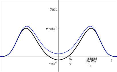
Figure 2: The potential of scalar field $U(\phi)$ in the gauge-mediated scheme of SUSY breaking at $\phi_{g}=\mu_{\mbox{\footnotesize{x}}}/\gamma$ and $\widetilde{m}\sim m_{\mathtt{Pl}}/\gamma$. The upper curve shows the potential with no supergravity corrections.

It is clear that $U(\phi)$ starts to rapidly grow from $U(0)$ at $\phi\sim\phi_{g}\sim\mu_{\mbox{\footnotesize{x}}}$, where $\mathcal{C}(\phi)$ effectively becomes to dominate with respect to unit. The potential begins to fall at $\phi\sim\sqrt{\widetilde{m}\,\phi_{g}}\sim\sqrt{m_{\mathtt{Pl}}\,\mu_{\mbox{\footnotesize{x}}}}\gg\mu_{\mbox{\footnotesize{x}}}$. Then, the characteristic change of field between two minima of potential is about $\delta\phi\sim\sqrt{m_{\mathtt{Pl}}\,\mu_{\mbox{\footnotesize{x}}}}$, which corresponds to thin domain wall.

Thus, the thin domain wall is relevant to the gauge-mediated SUSY breaking at low scales $\mu_{\mbox{\footnotesize{x}}}\sim 10^{4}$ GeV.

VI.2 Gravity-mediated SUSY breaking

If the gravity is responsible for the transition of SUSY breaking to the observed matter sector, the expansion of $\mathcal{C}$ is composed versus powers of Newtonian constant, i.e. in the inverse Planck mass. Therefore, to the leading order one expects

$$\mathcal{C}(\phi)\mapsto\frac{\bar{\gamma}^{2}\phi^{2}}{m_{\mathtt{Pl}}^{2}},\qquad\mbox{at }\bar{\gamma}\sim 1.$$ (63)

The leading term depends on the mass scale $\widetilde{m}_{\rm thick}$, which can be estimated by

$$\frac{\phi^{2}}{\hskip 5.0pt\widetilde{m}_{\rm thick}^{2}}\mapsto\frac{\phi^{2}\phi^{2}_{\mbox{\footnotesize{gr}}}}{m_{\mathtt{Pl}}^{4}},$$ (64)

where $\phi_{\mbox{\footnotesize{gr}}}\ll\mu_{\mbox{\footnotesize{x}}}$ denotes the characteristic scale of observed fields or superpartner masses, which is composed by breaking scale $\mu_{\mbox{\footnotesize{x}}}$, and it includes powers of inverse Planck mass, too. Therefore,

$$\widetilde{m}_{\rm thick}=\frac{m_{\mathtt{Pl}}^{2}}{\phi_{\mbox{\footnotesize{gr}}}},$$

while

$$\delta\phi\sim\sqrt{\widetilde{m}_{\rm thick}m_{\mathtt{Pl}}}.$$

For instance, at $\phi_{\mbox{\footnotesize{gr}}}\sim\mu_{\mbox{\footnotesize{x}}}^{2}/m_{\mathtt{Pl}}\sim\sqrt{G}\,\mu_{\mbox{\footnotesize{x}}}^{2}$ we find the distance between fields fitted to the minima of potential

$$\delta\phi\sim\frac{m_{\mathtt{Pl}}^{2}}{\mu_{\mbox{\footnotesize{x}}}},$$

while $\phi_{\mbox{\footnotesize{gr}}}\sim\mu_{\mbox{\footnotesize{x}}}^{3}/m_{\mathtt{Pl}}^{2}\sim G\,\mu_{\mbox{\footnotesize{x}}}^{3}$ corresponds to

$$\delta\phi\sim\frac{m_{\mathtt{Pl}}^{2}}{\mu_{\mbox{\footnotesize{x}}}}\sqrt{\frac{m_{\mathtt{Pl}}}{\mu_{\mbox{\footnotesize{x}}}}}.$$

Both above cases of $\phi_{\mbox{\footnotesize{gr}}}$ represent two known versions of standard scenario for the gravity-mediated SUSY breaking Weinberg-VIII .

Since the field is exposed to super-Planckian changes, we deal with thick domain walls in the gravity-mediated SUSY breaking at high scales about $10^{12-13}$ GeV.

To the end of this Section, we especially emphasize that at super-Planckian changes of field in thick domain walls, the height of potential barrier takes the values much less than the energy density of AdS vacuum, $V_{0}\ll\mu_{\mbox{\footnotesize{x}}}^{4}$. Therefore, one should control the dimensionless parameters like $\bar{\gamma}$ in order to get positive values of actual potential (62) within the wall. In this respect, one can see the role of presented potential as a toy model, that serves to demonstrate some general features of scale dependence in the problem. In practice, the form of true potential is strongly depends of the field contents in the theory. Moreover, remember that we have accented the attention on the nonperturbative low-energy contribution and neglected a tree potential.

VII Angle $\theta_{\tiny\textmd{K}}$

The mixing angle of two levels $\theta_{\mbox{\footnotesize{k}}}$ takes different values depending on the scenario of SUSY breaking.

For thin domain wall we get

$$\theta_{\mbox{\footnotesize{k}}}\approx\frac{\widetilde{\rho}}{\rho_{\mbox{\footnotesize{x}}}}\sim\frac{\mu_{\mbox{\footnotesize{x}}}^{2}}{m_{\mathtt{Pl}}^{2}}\sim\frac{\mu_{\Lambda}}{m_{\mathtt{Pl}}}.$$ (65)

Therefore, its value is certainly fixed by present day data on the cosmological constant, $\theta_{\mbox{\footnotesize{k}}}\sim 10^{-30}$.

In contrast, for thick domain walls we write down

$$\theta_{\mbox{\footnotesize{k}}}\approx\sqrt{\frac{\widetilde{\rho}^{2}}{\rho_{\mbox{\footnotesize{x}}}^{2}}}=\sqrt{\frac{\rho_{\Lambda}^{\rm dS}}{\rho_{\mbox{\footnotesize{x}}}}}\sim\frac{\mu_{\Lambda}^{2}}{\mu_{\mbox{\footnotesize{x}}}^{2}},$$ (66)

where $\mu_{\mbox{\footnotesize{x}}}$ depends on the scheme of gravity-mediated SUSY breaking. In the above examples we roughly get the estimate $\theta_{\mbox{\footnotesize{k}}}\sim 10^{-(46-48)}$.

VIII Generation problem

The vacuum states $|\Phi_{\mbox{\footnotesize{s}}}\rangle$ and $|\Phi_{\mbox{\footnotesize{x}}}\rangle$ are determined by classical values of scalar field in the local minima of its potential. So, the quantization of dynamical fields in vicinity of such vacua are straightforwardly standard. The question is how can we quantize the fields over the true vacuum being the superposition of such two states in accordance with (43)?

First, we can determine the field masses in vacua $|\Phi_{\mbox{\footnotesize{s}}}\rangle$ and $|\Phi_{\mbox{\footnotesize{x}}}\rangle$, respectively, in ordinary way. Say, let $m_{\mbox{\footnotesize{s}}}$ and $m_{\mbox{\footnotesize{x}}}$ be the masses of fermion field as given by such the procedure. Hence, the masses corresponds to the cases of exact and broken SUSY.

Second, the superposition of vacuum states is equivalently described by 2D vector or column

$$|\mbox{vac}\rangle\mapsto\left(\begin{array}[]{c}\cos\theta_{\mbox{\footnotesize{k}}}\\ \sin\theta_{\mbox{\footnotesize{k}}}\\ \end{array}\right).$$ (67)

Therefore, the mass term of fermion field should be given by $2\raisebox{1.0pt}{$\scriptstyle\times$}2$-matrix of general form

$$M=\left(\begin{array}[]{cl}m_{\mbox{\footnotesize{x}}}&\bar{m}\\[2.84526pt] \bar{m}&m_{\mbox{\footnotesize{s}}}\\ \end{array}\hskip-2.0pt\right).$$ (68)

It is clear that such the construction is responsible for two generations of the same field.

Thus, the vacuum structure in the form of superposition can be the origin of generations observed in the Standard Model. Then, one should suggest the superposition of three vacuum levels, at least. Probably, one could prefer for the situation with two flat vacua and signle AdS vacuum as it depicted in Fig. 2. Then, the hamiltonian of vacuum contains the mixing of AdS level with each flat state $|\Phi_{\mbox{\footnotesize{s}}}\rangle_{+}$ and $|\Phi_{\mbox{\footnotesize{s}}}\rangle_{-}$ at positive and negative values of flat minima, while the eigenstate relevant to our Universe takes the form of superposition

$$|\mbox{vac}\rangle_{\mbox{\footnotesize{3g}}}\approx\frac{1}{\sqrt{2}}\big{\{}|\mbox{vac}\rangle_{+}+|\mbox{vac}\rangle_{-}\big{\}},$$ (69)

which is represented as 3D vector

$$|\mbox{vac}\rangle_{\mbox{\footnotesize{3g}}}\mapsto\frac{1}{\sqrt{2}}\left(\begin{array}[]{c}2\sin\theta_{\mbox{\footnotesize{k}}}\\ \cos\theta_{\mbox{\footnotesize{k}}}\\ \cos\theta_{\mbox{\footnotesize{k}}}\\ \end{array}\hskip-2.0pt\right),$$ (70)

in the basis of states $\{|\Phi_{\mbox{\footnotesize{x}}}\rangle,|\Phi_{\mbox{\footnotesize{s}}}\rangle_{+},|\Phi_{\mbox{\footnotesize{s}}}\rangle_{-}\}$, that could be actual for 3 generations, probably, with some realistic textures of mass matrices of matter fields.

We finalize at this point, since the consideration of spectroscopy is beyond the scope of present paper. The problem is reduced to calculation of non-diagonal “masses” a la $\bar{m}$ in (68).

IX Conclusion

In this paper we have described the mechanism for dynamical generation of small cosmological constant due to seesaw mixing of two initial vacuum-states describing the phases of exact and broken supersymmetry. The current value of cosmological constant is consistent with phenomenological estimates of SUSY broken scale in particle physics.

The mechanism works due to fluctuations formed by bubbles of AdS vacuum separated by domain walls from the flat vacuum. We have classified the cases of thin and thick domain walls related with gauge or gravity-mediated SUSY breaking, respectively. The mixing results in the superposition of initial vacua, that could set the origin of three generations of fermions in the Standard Model.

Further studies of such the mechanism have to answer important questions on the spectroscopy of matter and superpartners as well as on a role of mixing angle $\theta_{\mbox{\footnotesize{k}}}$ and methods of its direct measurement. In addition, one should clarify why we are living in the vacuum we have got. An answer to this question could disfavor the scheme with two flat vacua as presented in Section VIII. Then, an inverse picture with two AdS-vacua and single flat vacuum could be more realistic. This possibility will be investigated elsewhere prepare-Inflat . Nevertheless, basic features of scale dependence found in the present paper, should remain valid with no changes.

References

-
(1)
A. G. Riess et al. [Supernova Search Team
Collaboration],
Astron. J. 116, 1009 (1998) [arXiv:astro-ph/9805201];
B. P. Schmidt et al. [Supernova Search Team Collaboration], Astrophys. J. 507, 46 (1998) [arXiv:astro-ph/9805200];
S. Perlmutter et al. [Supernova Cosmology Project Collaboration], Astrophys. J. 517, 565 (1999) [arXiv:astro-ph/9812133];
J. P. Blakeslee et al. [Supernova Search Team Collaboration], Astrophys. J. 589, 693 (2003) [arXiv:astro-ph/0302402];
A. G. Riess et al. [Supernova Search Team Collaboration], Astrophys. J. 560, 49 (2001) [arXiv:astro-ph/0104455]. - (2) A. G. Riess et al. [Supernova Search Team Collaboration], Astrophys. J. 607, 665 (2004) [arXiv:astro-ph/0402512].
- (3) P. Astier et al., arXiv:astro-ph/0510447.
-
(4)
D. N. Spergel et al. [WMAP Collaboration],
Astrophys. J. Suppl. 148, 175 (2003)
[arXiv:astro-ph/0302209];
D. N. Spergel et al., arXiv:astro-ph/0603449. -
(5)
D. J. Eisenstein et al.,
arXiv:astro-ph/0501171;
S. Cole et al. [The 2dFGRS Collaboration], Mon. Not. Roy. Astron. Soc. 362, 505 (2005) [arXiv:astro-ph/0501174]. -
(6)
T. Chiba,
Phys. Rev. D 60, 083508 (1999)
[arXiv:gr-qc/9903094];
N. A. Bahcall, J. P. Ostriker, S. Perlmutter and P. J. Steinhardt, Science 284, 1481 (1999) [arXiv:astro-ph/9906463];
P. J. Steinhardt, L. M. Wang and I. Zlatev, Phys. Rev. D 59, 123504 (1999) [arXiv:astro-ph/9812313];
L. M. Wang, R. R. Caldwell, J. P. Ostriker and P. J. Steinhardt, Astrophys. J. 530, 17 (2000) [arXiv:astro-ph/9901388]. - (7) V. Sahni and A. Starobinsky, Int. J. Mod. Phys. D 15, 2105 (2006) [arXiv:astro-ph/0610026].
- (8) S. Weinberg, Rev. Mod. Phys. 61, 1 (1989).
- (9) I. Y. Kobzarev, L. B. Okun and M. B. Voloshin, Sov. J. Nucl. Phys. 20, 644 (1975) [Yad. Fiz. 20, 1229 (1974)]; S. R. Coleman, Phys. Rev. D 15, 2929 (1977) [Erratum-ibid. D 16, 1248 (1977)]; C. G. Callan and S. R. Coleman, Phys. Rev. D 16, 1762 (1977).
- (10) S. R. Coleman and F. De Luccia, Phys. Rev. D 21, 3305 (1980).
- (11) S. Weinberg, Phys. Rev. Lett. 48, 1776 (1982).
- (12) H. Fritzsch, Phys. Lett. B 70, 436 (1977); H. Harari, H. Haut and J. Weyers, Phys. Lett. B 78, 459 (1978); H. Fritzsch, Nucl. Phys. B 155, 189 (1979); Y. Koide, Phys. Rev. D 28, 252 (1983); P. Kaus and S. Meshkov, Mod. Phys. Lett. A 3, 1251 (1988) [Erratum-ibid. A 4, 603 (1989)]; Y. Koide, Phys. Rev. D 39, 1391 (1989); H. Fritzsch and J. Plankl, Phys. Lett. B 237, 451 (1990).
- (13) E. Witten, Nucl. Phys. B 202, 253 (1982).
- (14) S. Weinberg, “The quantum theory of fields”, Volume III “Supersymmetry”, Cambridge University Press, 2000.
- (15) W. Nahm, Nucl. Phys. B 135, 149 (1978).
- (16) A. A. Andrianov, F. Cannata, P. Giacconi, A. Y. Kamenshchik and R. Soldati, Phys. Lett. B 651, 306 (2007) [arXiv:0704.1436 [gr-qc]].
- (17) T. Banks, arXiv:hep-th/0211160.
- (18) M. McGuigan, arXiv:hep-th/0602112; hep-th/0604108.
- (19) K. Enqvist, S. Hannestad and M. S. Sloth, Phys. Rev. Lett. 99, 031301 (2007) [arXiv:hep-ph/0702236].
- (20) T. Banks, arXiv:hep-th/0007146.
- (21) V. V. Kiselev and S. A. Timofeev, in preparation.