Physical and Geometrical Interpretation of the $\epsilon\leq 0$ Szekeres Models.

Abstract

We study the properties and behaviour of the quasi-pseudospherical and quasi-planar Szekeres models, obtain the regularity conditions, and analyse their consequences. The quantities associated with “radius” and “mass” in the quasi-spherical case must be understood in a different way for these cases. The models with pseudospherical foliation can have spatial maxima and minima, but no origins. The “mass” and “radius” functions may be one increasing and one decreasing without causing shell crossings. This case most naturally describes a snake-like, variable density void in a more gently varying inhomogeneous background, although regions that develop an overdensity are also possible. The Szekeres models with plane foliation can have neither spatial extrema nor origins, cannot be spatially flat, and they cannot have more inhomogeneity than the corresponding Ellis model, but a planar surface can be the boundary between regions of spherical and pseudospherical foliation.

I Introduction

The Szekeres metric is important because, as a model with 5 arbitrary functions, it exhibits features of non-linear gravitation that less general models cannot. It is an exact inhomogeneous solution of the Einstein field equations (EFEs) that has a realistic equation of state (dust) suitable for the post recombination universe, it has no Killing vectors. It is necessary to pay more attention to models with little symmetry in order to better understand all the features and possibilities of General Relativity, and therefore to better model the structures of our universe.

Although there have been a number of papers that investigate the Szekeres metric generally Szek1975a ; BoTo1976 ; GoWa1982a ; GoWa1982b , and several papers that investigate the quasi-spherical case in particular Szek1975b ; Bonn1976a ; BoST1977 ; Bonn1976b ; DeSo1985 ; Bonn1986 ; BoPu1987 ; Szek1980 , there have been none that specifically look at the quasi-pseudospherical and quasi-planar cases. This is probably because we have a good understanding of spherical gravity from Newtonian theory, and so relativistic analyses of spherically symmetric metrics were easily developed. Without spherical symmetry, or a slight variation of it, familiar relationships, such as that between the mass inside a sphere and the gravitational potential, do not apply, so it is much more difficult to interpret the equations physically.

We here set out to improve our understanding of the quasi-planar and quasi-pseudospherical models, and thus enhance their usability, by analysing their physical and geometric properties. The main challenge is to develop a re-interpretation of quantities such as “radius” and “mass” that cannot retain the meaning they have in (nearly) spherical models.

The appearance of the first paper Bole2006 to produce an explicit model using the quasi-spherical Szekeres metric, that of a void adjacent to a cluster, and to plot the evolution of its density, is an encouraging development. If the other Szekeres cases are sufficiently well understood, explicit models can be produced from these too.

Our methods below are to (a) analyse how the metric functions affect the geometry, the matter distribution, and the evolution, (b) derive regularity conditions on the metric for well behaved matter, curvature and evolution, (c) compare with other metrics that have planar and pseudospherical symmetry, and (d) produce one or two simple examples.

II The Szekeres Metric

In this section we will present the metric and its basic relationships, but we will refrain from any physical interpretation, reserving that for a later section. Once all the features and properties of the model are established, we will collect the results, discuss the meaning of the various functions, and attempt an interpretation of the model.

Our notation is that of HeKr2002 , for which this is a follow up. The LT-type Szekeres metric Szek1975a ; Szek1975b ; Kras1997 ; PlKr2006 is:

$$ds^{2}=-dt^{2}+\frac{(R^{\prime}-R\frac{\textstyle E^{\prime}}{\textstyle E})^{2}}{(\epsilon+f)}dr^{2}+R^{2}\frac{(dp^{2}+dq^{2})}{E^{2}}~{},$$ (1)

where ${}^{\prime}\equiv\partial/\partial r$, $\epsilon=\pm 1,0$ and $f=f(r)\geq-\epsilon$ is an arbitrary function of $r$. The function $E$ is given by

$$E(r,p,q) =\frac{S}{2}\left\{\left(\frac{p-P}{S}\right)^{2}+\left(\frac{q-Q}{S}\right)^{2}+\epsilon\right\}~{},$$ (2)

$$\epsilon =0,\pm 1~{},$$

where $S=S(r)$, $P=P(r)$, and $Q=Q(r)$ are arbitrary functions. In the original parametrisation of Szekeres, $E$ had the form

$$E(r,p,q)=A(p^{2}+q^{2})+2B_{1}p+2B_{2}q+C~{},$$ (3)

where

$$A =\frac{1}{2S}~{},~{}~{}B_{1}=\frac{-P}{2S}~{},~{}~{}B_{2}=\frac{-Q}{2S}~{},$$

$$C =\frac{P^{2}+Q^{2}+\epsilon S^{2}}{2S}~{},~{}~{}4(AC-B_{1}^{2}-B_{2}^{2})=\epsilon~{}.$$ (4)

The function $R=R(t,r)$ satisfies the Friedmann equation for dust

$$\dot{R}^{2}=\frac{2M}{R}+f,$$ (5)

where $\dot{{}}\equiv\partial/\partial t$ and $M=M(r)$ is another arbitrary function of coordinate $r$. It follows that the acceleration of $R$ is

$$\ddot{R}=\frac{-M}{R^{2}}.$$ (6)

Solving (5), the evolution of $R$ depends on the value of $f$; it can be:
  hyperbolic, $f>0$:

$$R =\frac{M}{f}(\cosh\eta-1)~{},$$ (7)

$$(\sinh\eta-\eta) =\frac{f^{3/2}\sigma(t-a)}{M}~{},$$ (8)

  parabolic, $f=0$:

$$R=\left(\frac{9M(t-a)^{2}}{2}\right)^{1/3}~{},$$ (9)

  or elliptic, $f<0$:

$$R =\frac{M}{(-f)}(1-\cos\eta)~{},$$ (10)

$$(\eta-\sin\eta) =\frac{(-f)^{3/2}\sigma(t-a)}{M}~{},$$ (11)

where $a=a(r)$ is the last arbitrary function, giving the local time of the big bang or crunch $R=0$ and $\sigma=\pm 1$ permits time reversal. More correctly, the three types of evolution hold for $f/M^{2/3}>,=,<0$, since $f=0$ at a spherical type origin for all 3 evolution types. The behaviour of $R(t,r)$ is identical to that in the Lemaître-Tolman (LT) model, and is unaffected by $(p,q)$ variations.

The 6 arbitrary functions $f$, $M$, $a$, $S$, $P$ and $Q$ give us 5 functions to control the physical inhomogeneity, plus a choice of the coordinate $r$. Note, however, that in the case $\epsilon=0$ we are free to redefine the functions $R$, $S$, $f$ and $M$ as follows:

$$(R,S,f,M)=(\alpha\widetilde{R},\widetilde{S}/\alpha,\alpha^{2}\widetilde{f},\alpha^{3}\widetilde{M}),$$ (12)

where $\alpha=\alpha(r)$ is an arbitrary function, and the form of the metric, the density and the evolution equations will not change. In particular, we can choose $\alpha$ so that $\widetilde{S}=1$.

The density and Kretschmann scalar are functions of all four coordinates

$$8\pi\rho =G_{tt}=\frac{2(M^{\prime}-3ME^{\prime}/E)}{R^{2}(R^{\prime}-RE^{\prime}/E)},$$ (13)

$${\cal K} =R^{\alpha\beta\gamma\delta}R_{\alpha\beta\gamma\delta}=(8\pi)^{2}\left[\frac{4}{3}\overline{\rho}^{2}-\frac{8}{3}\overline{\rho}\rho+3\rho^{2}\right],$$ (14)

where

$$8\pi\overline{\rho}=\frac{6M}{R^{3}}$$ (15)

is some kind of mean density. For all $\rho$ and $\overline{\rho}$ we have ${\cal K}\geq 0$, but assumptions of positive mass and density require $\rho\geq 0$ and $\overline{\rho}\geq 0$. The flow properties of the comoving matter were given for any $\epsilon$ value in HeKr2002 . For further discussion of this metric see Kras1997 ; PlKr2006 .

In the following, we will call the comoving surfaces of constant $r$ “shells”, and paths that follow constant $p$ & $q$ will be termed “radial”. We will use the term “hyperbolic” to describe the time evolution for $f>0$, and “pseudospherical” or “hyperboloidal” to describe the shape of the $(p,q)$ 2-surfaces when $\epsilon=-1$. To make it clear the shells are quite different from spheres, we will call $r$ the “p-radius” or “h-radius”, $R$ the “areal p-radius” or “areal h-radius’, and $M$ the “p-mass” or “h-mass”, in the planar or pseudospherical cases, respectively. However, we will use “radius” generically when more than one $\epsilon$ value is considered.

II.1 Singularities

The bang or crunch occur when $t=a$ or $t=2\pi M/(-f)^{3/2}+a$, which makes $R=0$ and both $\rho$ and $\cal K$ divergent. Shell crossings happen when surfaces (“shells”) of different $r$ values intersect, i.e. $R^{\prime}=RE^{\prime}/E$ and $M^{\prime}\neq 3ME^{\prime}/E$. Also $\rho$ but not ${\cal K}$ passes through zero where $E^{\prime}/E$ exceeds $M^{\prime}/3M$.

II.2 Special Cases and Limits

The Lemaître-Tolman model is the spherically symmetric special case $\epsilon=+1$, $E^{\prime}=0$.

The Ellis metrics Elli1967 result as the special case $E^{\prime}=0$; they are the LT model and its counterparts with plane and pseudospherical symmetry.

The vacuum case is $(M^{\prime}-3ME^{\prime}/E)=0$, which implies $E^{\prime}=M^{\prime}=0=S^{\prime}=P^{\prime}=Q^{\prime}$. For $M\neq 0$ this gives pseudospherical and planar equivalents of the Schwarzschild metric CaDe1968 (see section VI.2).

The null limit is obtained by taking $f\rightarrow\infty$ after a suitable tranformation. In this limit the ‘dust’ particles move at light speed Hel96 ; Bon97 and the metric becomes a pure radiation Robinson-Trautman metric of Petrov type D (see SKMHH03 eq (28.71) with (28.73)).

The Kantowski-Sachs (KS) type Szekeres metric is in fact a regular limit of the LT type Szekeres metric Hel96 ; PlKr2006 .

II.3 Basic Physical Restrictions

1. In order to keep the metric signature Lorentzian we must have

   $$\epsilon+f\geq 0~{},$$ (16)

   and in particular

   $$\epsilon+f>0~{}~{}~{}~{}\mbox{and}~{}~{}~{}~{}R^{\prime}-\frac{RE^{\prime}}{E}\neq 0~{},$$ (17)

   while

   $$\epsilon+f=0~{}~{}~{}~{}\mbox{where}~{}~{}~{}~{}R^{\prime}=\frac{RE^{\prime}}{E}~{}.$$ (18)

   Clearly, pseudospherical foliations, $\epsilon=-1$, require $f\geq 1$, and so are only possible for regions with hyperbolic evolution, $f>0$. Similarly, planar foliations, $\epsilon=0$, are only possible for regions with parabolic or hyperbolic evolution, $f\geq 0$; whereas spherical foliations are possible for all $f\geq-1$.

2. We require the metric to be non degenerate & non singular, except at the bang or crunch. For a well behaved $r$ coordinate then, we need to specify

   $$\infty>\frac{(R^{\prime}-RE^{\prime}/E)^{2}}{(\epsilon+f)}>0~{}.$$ (19)

   Whilst failure to satisfy this may only be due to bad coordinates, there should exist a choice of $r$ coordinate for which it holds.

3. The density must be positive, and the Kretschmann scalar must be finite, i.e.

   $$\infty>\frac{M^{\prime}-3ME^{\prime}/E}{R^{\prime}-RE^{\prime}/E}\geq 0~{}.$$ (20)

4. We assume

   $$R\geq 0~{},~{}~{}~{}~{}M\geq 0~{}~{}~{}~{}\mbox{and}~{}~{}~{}~{}S>0~{}.$$ (21)

   The sign of $S$, and hence of $E$ can be flipped without changing the metric, but $S=0$ is not acceptable.

5. The various arbitrary functions should have sufficient continuity — $C^{1}$ and piecewise $C^{3}$ — except possibly at a spherical origin.

II.4 3-spaces of constant $t$

It is known from BeEaOl77 that when $\epsilon=+1$ these 3-spaces are conformally flat, and it is easy to verify, using Maple Maple and GRTensor GRT that the Cotton-York tensor is zero for all $\epsilon$ (see PlKr2006 , section 19.11, exercise 19.14, and theorem 7.1).

Calculating the Riemann tensor for the constant $t$ spatial sections of (1), we find

$${}^{3}\!R_{rprp} ={}^{3}\!R_{rqrq}$$

$$=\frac{-R}{E^{2}(\epsilon+f)}\left(R^{\prime}-\frac{RE^{\prime}}{E}\right)\left(\frac{f^{\prime}}{2}-\frac{fE^{\prime}}{E}\right)$$ (22)

$${}^{3}\!R_{pqpq} =\frac{-R^{2}f}{E^{4}}$$ (23)

$${}^{3}\!R =\frac{2f}{R^{2}}\left(\frac{2\left(\frac{f^{\prime}}{2f}-\frac{E^{\prime}}{E}\right)}{\left(\frac{R^{\prime}}{R}-\frac{E^{\prime}}{E}\right)}+1\right)$$ (24)

$${}^{3}{\cal K} ={}^{3}\!R^{ijkl}{}^{3}\!R_{ijkl}=\frac{4f^{2}}{R^{4}}\left(\frac{2\left(\frac{f^{\prime}}{2f}-\frac{E^{\prime}}{E}\right)^{2}}{\left(\frac{R^{\prime}}{R}-\frac{E^{\prime}}{E}\right)^{2}}+1\right)$$ (25)

where equations (2)-(5) of Hel96 have been used, and the other curvature invariants are linearly dependent on these. The flatness condition ${}^{3}\!R_{abcd}=0$ requires

$$\epsilon \neq 0:~{}~{} f=0$$ (26)

$$\epsilon =0:~{}~{} R^{\prime}=E^{\prime}=f^{\prime}=f=0$$ (27)

and the latter is only possible as a limit, or as a Kantowski-Sachs type Szekeres model Hel96b . Interestingly, $(\epsilon+f)$ does not enter any curvature invariants, and they are all well behaved if $f=0$. The 2-spaces of constant $t$ and $r$ have Ricci scalar

$${}^{2}\!R =\frac{2\epsilon}{R^{2}}~{}.$$ (28)

II.5 General properties of $E(r,p,q)$

From (2) we see $E$ has circular symmetry about $p=P$, $q=Q$, which is a different point for each $r$. The $E=0$ locus

$$(p-P)^{2}+(q-Q)^{2}=-\epsilon S^{2}~{},$$ (29)

only exists if $\epsilon\leq 0$, and is clearly a circle in the $p$-$q$ plane, with $E>0$ on the outside, but becomes a point $p=P$, $q=Q$ if $\epsilon=0$. We have

$$E^{\prime} =-\frac{S^{\prime}}{2}\left\{\left(\frac{p-P}{S}\right)^{2}+\left(\frac{q-Q}{S}\right)^{2}-\epsilon\right\}$$

$$~{}~{}~{}~{}-\left(\frac{p-P}{S}\right)P^{\prime}-\left(\frac{q-Q}{S}\right)Q^{\prime}$$ (30)

so the $E^{\prime}=0$ locus is also a circle in the $p$-$q$ plane, since it can be written

$$\left(\frac{p-P}{S}+\frac{P^{\prime}}{S^{\prime}}\right)^{2}+\left(\frac{q-Q}{S}+\frac{Q^{\prime}}{S^{\prime}}\right)^{2}=\frac{(P^{\prime})^{2}+(Q^{\prime})^{2}}{(S^{\prime})^{2}}+\epsilon~{}.$$ (31)

With $\epsilon\geq 0$, this locus always exists, and with $\epsilon=-1$ it only exists if

$$(S^{\prime})^{2}<(P^{\prime})^{2}+(Q^{\prime})^{2}~{},$$ (32)

with the radius of this circle shrinking to zero as the equality is approached. Since, if they exist, the distance between the centres of these two circles never exceeds the sum of their radii

$$\left|\frac{S}{S^{\prime}}\right| \sqrt{(P^{\prime})^{2}+(Q^{\prime})^{2}}\;\leq$$

$$\left|\frac{S}{S^{\prime}}\right|\left(\left|S^{\prime}\right|\sqrt{-\epsilon}\;+\sqrt{(P^{\prime})^{2}+(Q^{\prime})^{2}+\epsilon(S^{\prime})^{2}}\;\right)$$ (33)

they always intersect, and the intersection points are

$$\frac{p-P}{S} =\frac{\epsilon P^{\prime}S^{\prime}\pm Q^{\prime}\sqrt{-\epsilon\left\{(P^{\prime})^{2}+(Q^{\prime})^{2}+\epsilon(S^{\prime})^{2}\right\}}\;}{(P^{\prime})^{2}+(Q^{\prime})^{2}\;}~{},$$

$$\frac{q-Q}{S} =\frac{\epsilon Q^{\prime}S^{\prime}\mp P^{\prime}\sqrt{-\epsilon\left\{(P^{\prime})^{2}+(Q^{\prime})^{2}+\epsilon(S^{\prime})^{2}\right\}}\;}{(P^{\prime})^{2}+(Q^{\prime})^{2}\;}~{}.$$ (34)

To see how $E^{\prime}/E$ affects the metric and the density, we write $x=E^{\prime}/E$. Then in the metric (1), $g_{rr}$ is a decreasing function of $x$ provided $x>R^{\prime}/R$, while for the density (13) we have

$$8\pi\rho =\frac{6M}{R^{3}}\,\frac{(M^{\prime}/(3M)-x)}{(R^{\prime}/R-x)}~{},$$ (35)

so that

$$8\pi\frac{\partial{\rho}}{\partial{x}} =-\frac{6M}{R^{3}}\frac{(R^{\prime}/R-M^{\prime}/(3M))}{(R^{\prime}/R-x)^{2}}$$ (36)

and if $$x\to\pm\infty$$

$$8\pi\rho \to\frac{6M}{R^{3}}~{}.$$ (37)

Therefore at given $r$ and $t$ values, the density varies monotonically with $x=E^{\prime}/E$, but the sign of the numerator may possibly change as $R$ evolves. If $x$ can diverge, $\rho$ approaches a finite, positive limit.

The metric component

$$\frac{(dp^{2}+dq^{2})}{E^{2}}$$ (38)

is a 2-d surface of constant unit curvature, that is a pseudosphere, a plane, or a sphere in Riemann or stereographic projection:

$$\epsilon=-1~{},~{}E>0:~{}~{}\frac{(p-P)}{S}=\coth\left(\frac{\theta}{2}\right)\cos(\phi)~{},$$

$$~{}~{}~{}~{}~{}~{}\frac{(q-Q)}{S}=\coth\left(\frac{\theta}{2}\right)\sin(\phi)~{},$$ (39)

$$\epsilon=-1~{},~{}E<0:~{}~{}\frac{(p-P)}{S}=\tanh\left(\frac{\theta}{2}\right)\cos(\phi)~{},$$

$$~{}~{}~{}~{}~{}~{}\frac{(q-Q)}{S}=\tanh\left(\frac{\theta}{2}\right)\sin(\phi)~{},$$ (40)

$$\epsilon=~{}0:~{}~{}\frac{(p-P)}{S}=\left(\frac{2}{\theta}\right)\cos(\phi)~{},$$

$$~{}~{}~{}~{}~{}~{}\frac{(q-Q)}{S}=\left(\frac{2}{\theta}\right)\sin(\phi)~{},$$ (41)

$$\epsilon=+1:~{}~{}\mbox{either}~{}~{}\frac{(p-P)}{S}=\cot\left(\frac{\theta}{2}\right)\cos(\phi)~{},$$

$$~{}~{}~{}~{}~{}~{}\frac{(q-Q)}{S}=\cot\left(\frac{\theta}{2}\right)\sin(\phi)~{}.$$ (42)

$$\mbox{or}~{}~{}~{}~{}~{}~{}~{}~{}~{}~{}~{}~{}~{}~{}~{}~{}~{}~{}~{}~{}\frac{(p-P)}{S}=\tan\left(\frac{\theta}{2}\right)\cos(\phi)~{},$$

$$~{}~{}~{}~{}~{}~{}\frac{(q-Q)}{S}=\tan\left(\frac{\theta}{2}\right)\sin(\phi),$$ (43)

Figure 1: The Riemann projection from $(\theta,\phi)$ to $(p,q)$ coordinates for pseudospheres ($\epsilon=-1$). The projections of the two sheets require different formulae, one is shown as solid grey lines, the other as dark dashed lines. The $45^{\circ}$ asymptotes that divide the projections of the two hyperboloid sheets are shown as dot-dash lines. This and the next 2 diagrams show only the $\phi=0,\pi$ section, i.e. the $q=Q$ section. For the full projection, they should be rotated around the $z$ axis and the $q$ dimension added.

Figure 2: The Riemann projection from $(\theta,\phi)$ to $(p,q)$ coordinates for semi-infinite cylinders ($\epsilon=0$). Section V.3 gives the projection as an inversion of the plane in a circle, which can’t be illustrated as above. The diagram here shows the projection of a cylinder, with $\theta$ increasing along the length of the cylinder, and each half cylinder maps to the full $(p,q)$ plane (with the same formula).

Figure 3: The Riemann projection from $(\theta,\phi)$ to $(p,q)$ coordinates for spheres ($\epsilon=+1$). Each of the two possible projection formulae maps the full sphere to the plane, but only half of each is shown, one as solid grey lines, the other as dark dashed lines.

Figure 4: The relation bewtween $p$ & $\theta$ for each of the Szekeres types. Only $(p-P)\geq 0$ and $\theta>0$ is shown, as rotating $\phi$ completes the mapping. The dark dot-dash line is for $\epsilon=+1$, the pale solid line is for $\epsilon=0$, and medium dashed line is for $\epsilon=-1$.

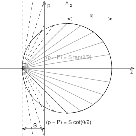
The projections are illustrated in figs 1-3, and the $\theta$-to-$p$ transformations (at $\phi=0$) are shown in fig 4. In these diagrams, the parametric equations for spheres and right hyperboloids are

$$x =a\sin\theta\cos\phi~{},~{}~{}y=a\sin\theta\sin\phi~{},~{}~{}z=a\cos\theta~{},$$

$$~{}~{}~{}~{}~{}~{}0\leq\theta\leq\pi~{},~{}~{}0\leq\phi\leq 2\pi~{},$$ (44)

$$x =a\cos\phi~{},~{}~{}y=a\sin\phi~{},~{}~{}z=a\theta~{},$$

$$~{}~{}~{}~{}~{}~{}0\leq\theta\leq\infty~{},~{}~{}0\leq\phi\leq 2\pi~{},$$ (45)

$$x =a\sinh\theta\cos\phi~{},~{}~{}y=a\sinh\theta\sin\phi~{},~{}~{}z=a\cosh\theta~{},$$

$$~{}~{}~{}~{}~{}~{}-\infty\leq\theta\leq\infty~{},~{}~{}0\leq\phi\leq 2\pi~{},$$ (46)

where the former gives the entire sphere minus one point, but the latter gives only one sheet of the hyperboloid. Notice that, with $\theta$ & $\phi$ ranging over the whole sphere, each of the spherical transformations (39) & (40) covers the entire $p$-$q$ plane. (In fig 3, only the range $0\leq\theta\leq\pi/2$, $\phi=0,\pi$ has been shown for each.) In contrast, BOTH of the pseudospherical transformations (42) & (43), with $0\leq\theta\leq\infty$, are required to cover the entire $p$-$q$ plane once, each transformation mapping one of the hyperboloid sheets to the $p$-$q$ plane. To distinguish the sheets, we choose $\theta$ to be negative on one and positive on the other. In the planar case, the Riemann projection can be considered an inversion of the plane in a circle, which is hard to illustrate, or as in fig 2 a mapping of a semi-infinite cylinder to a plane.

One might suspect that the two regions of the $(p,q)$ plane on either side of $E=0$ simply provide a double covering of the same surface, but this is not the case. For the double-sheeted hyperboloid at a single $r$ value, the two sheets are isometric to each other, the isometry transformation $(p,q)\to(p^{\prime},q^{\prime})$ is

$$p =P_{0}+\frac{{S_{0}}^{2}(p^{\prime}-P_{0})}{(p^{\prime}-P_{0})^{2}+(q^{\prime}-Q_{0})^{2}},$$

$$q =Q_{0}+\frac{{S_{0}}^{2}(q^{\prime}-Q_{0})}{(p^{\prime}-P_{0})^{2}+(q^{\prime}-Q_{0})^{2}},$$ (47)

where $(S_{0},P_{0},Q_{0})$ are the values of $P$, $Q$ and $S$ in that hyperboloid. However, for a family of hyperboloids immersed in a Szekeres spacetime, the transformation (II.5) will change the values of the functions $(P,Q,S)$ in all other hyperboloids, and will not be an isometry. Thus, the two sheets are distinct surfaces in spacetime.

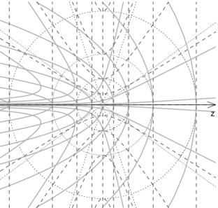
It is a property of the Riemann projection that for $\epsilon\geq 0$, circles in $(p,q)$ map to circles in $(\theta,\phi)$. Constant $\phi$ lines in $(\theta,\phi)$ (that obviously pass through $\theta=0$) map to straight lines through $p=P$, $q=Q$. Circles in $(\theta,\phi)$ that pass through $\theta=0$, map to straight lines in $(p,q)$. See fig. 5 for an example with $\epsilon=0$. For $\epsilon=0$ the projection is just an inversion of the plane in the circle of radius $\sqrt{2S}$.

Figure 5: An inversion with respect to the circle IC centred at CI maps an infinite straight line into a circle that passes through CI. The straight lines $l_{1}$, $l_{2}$ and $l_{3}$ are mapped into the circles $C_{1}$, $C_{2}$ and $C_{3}$, respectively. The straight line $l_{4}$ that passes through CI is mapped onto itself, i.e. the image-circle has then an infinite radius. A strip between two parallel straight lines is mapped into the crescent-shaped ring between their image-circles. The ring has finite surface area except when one edge of the strip passes through CI.

Thus the factor $\epsilon$ determines whether the $p$-$q$ 2-surfaces are pseudospherical ($\epsilon=-1$), planar ($\epsilon=0$), or spherical ($\epsilon=+1$). In other words, it determines the shape of the constant $r$ 2-surfaces that foliate the 3-d spatial sections of constant $t$. The function $E$ determines how the coordinates $(p,q)$ map onto the 2-d unit pseudosphere, plane or sphere at each value of $r$. Each 2-surface is multiplied by factor $R=R(t,r)$ that is different for each $r$ and evolves with time. Thus the $r$-$p$-$q$ 3-surfaces are constructed out of a sequence of 2-dimensional spheres, pseudospheres, or planes that are not arranged symmetrically. Obviously, for $\epsilon\leq 0$ the area of the $(t=$ const, $r=$const$)$ surfaces could be infinite, but in the $\epsilon=+1$ case it is $4\pi R^{2}$.

III The Effect of $\epsilon$ and $E$

We here analyse the role $E$ plays in these models, and contrast it with the $\epsilon=+1$ case, in which $E^{\prime}/E$ creates a dipole variation around the constant $(t,r)$ 2-spheres. We omit some of the detail below because very similar calculations were done in HeKr2002 . We assume $S>0$.

III.1 Pseudospherical foliations, $\epsilon=-1$

Transforming (2) and its derivatives using (39) and (40), and putting $\epsilon=-1$ , we get

$$E =\frac{\nu\,S}{\cosh\theta-\nu}~{},$$ (48)

$$E^{\prime} =-\frac{S^{\prime}\cosh\theta+\sinh\theta(P^{\prime}\cos\phi+Q^{\prime}\sin\phi)}{\cosh\theta-\nu}~{},$$ (49)

$$E^{\prime\prime} =-\frac{S^{\prime\prime}\cosh\theta+\sinh\theta(P^{\prime\prime}\cos\phi+Q^{\prime\prime}\sin\phi)}{(\cosh\theta-\nu)}$$

$$~{}~{}~{}~{}+2\left(\frac{S^{\prime}}{S}\right)\left(\frac{S^{\prime}\cosh\theta+\sinh\theta(P^{\prime}\cos\phi+Q^{\prime}\sin\phi)}{(\cosh\theta-\nu)}\right)$$

$$~{}~{}~{}~{}-\frac{((S^{\prime})^{2}-(P^{\prime})^{2}-(Q^{\prime})^{2})}{S}~{},$$ (50)

where $\nu=+1$ when $E>0$,  $0$ when $E=0$  and $-1$ when $E<0$. The $E=0$ circle corresponds to $\theta\to\pm\infty$, and its neighbourhood represents the asymptotic regions of the two sheets. It is clear that curves and regions that intersect the $E=0$ circle must have infinite length or area, since

$$L=\int\frac{R}{E}\sqrt{dp^{2}+dq^{2}}\;ds~{},~{}~{}~{}~{}A=\int\int\frac{R^{2}}{E^{2}}\,dp\,dq$$ (51)

The locus $E^{\prime}=0$ for all $E$ is

$$S^{\prime}\cosh\theta+P^{\prime}\sinh\theta\cos\phi+Q^{\prime}\sinh\theta\sin\phi=0~{}.$$ (52)

Writing $z=\cosh\theta$, $y=\sinh\theta\sin\phi$, $x=\sinh\theta\cos\phi$ as the parametric locus of a unit right hyperboloid centered on $(0,0,0)$ in flat 3-d space, we find (52) becomes $S^{\prime}z+P^{\prime}x+Q^{\prime}y=0$ which is a plane through $(0,0,0)$, so $E^{\prime}=0$ is the intersection of a plane with a right hyperboloid. In fact, (52) is a geodesic of the $p$-$q$ 2-space, as shown in appendix A.

We can write the $E^{\prime}=0$ locus as

$$\tanh\theta =\frac{-S^{\prime}}{P^{\prime}\cos\phi+Q^{\prime}\sin\phi}=\frac{-d}{\cos(\phi-\phi_{0})}$$ (53)

where

$$d =\frac{S^{\prime}}{\sqrt{(P^{\prime})^{2}+(Q^{\prime})^{2}}\;}~{},~{}~{}~{}~{}\tan(\phi_{0})=\frac{Q^{\prime}}{P^{\prime}}$$ (54)

so obviously a solution only exists if (32) holds, and only for

$$|\cos(\phi-\phi_{0})|\geq d~{}.$$ (55)

From (49) and (48) we find

$$\frac{E^{\prime}}{E}=-\nu\,\frac{S^{\prime}\cosh\theta+\sinh\theta(P^{\prime}\cos\phi+Q^{\prime}\sin\phi)}{S}~{},$$ (56)

thus $E^{\prime}/E=$ constant implies $S^{\prime}z+P^{\prime}x+Q^{\prime}y=S\times$ constant, which is a plane parallel to the $E^{\prime}=0$ plane. The location of the extrema of $E^{\prime}/E$ are found as follows

$$\frac{\partial(E^{\prime}/E)}{\partial\phi} =\nu\,\frac{\sinh\theta(P^{\prime}\sin\phi-Q^{\prime}\cos\phi)}{S}=0$$ (57)

$$\Rightarrow~{}~{}\tan\phi_{e}=\frac{Q^{\prime}}{P^{\prime}}~{}~{}~{}~{}\mbox{and}$$

$$\cos\phi_{e}=\epsilon_{1}\frac{P^{\prime}}{\sqrt{(P^{\prime})^{2}+(Q^{\prime})^{2}}\;}~{},$$ (58)

$$\frac{\partial(E^{\prime}/E)}{\partial\theta} =0=$$

$$-\nu \,\frac{S^{\prime}\sinh\theta+\cosh\theta(P^{\prime}\cos\phi+Q^{\prime}\sin\phi)}{S}$$ (59)

$$\Rightarrow~{}~{}\tanh\theta_{e}=-\frac{P^{\prime}\cos\phi_{e}+Q^{\prime}\sin\phi_{e}}{S^{\prime}}$$

$$~{}~{}~{}~{}~{}~{}~{}~{}=-\epsilon_{1}\frac{\sqrt{(P^{\prime})^{2}+(Q^{\prime})^{2}}\;}{S^{\prime}}~{}~{}~{}~{}\mbox{and}$$

$$\cosh\theta_{e}=\epsilon_{2}\frac{S^{\prime}}{\sqrt{(S^{\prime})^{2}-(P^{\prime})^{2}-(Q^{\prime})^{2}}\;}~{}.$$ (60)

where $\epsilon_{1}=\pm 1$ and $\epsilon_{2}={\rm sign}(S^{\prime})$. The extreme value is then

$$\left(\frac{E^{\prime}}{E}\right)_{\rm extreme}=-\epsilon_{2}\,\nu\frac{\sqrt{(S^{\prime})^{2}-(P^{\prime})^{2}-(Q^{\prime})^{2}}}{S}.$$ (61)

and these extrema only exist at finite $\theta$ if

$$(S^{\prime})^{2}>(P^{\prime})^{2}+(Q^{\prime})^{2}$$ (62)

which is the opposite of (32); so on a given constant $r$ shell, either $E^{\prime}=0$ exists, or the extrema of $E^{\prime}/E$ exist, but not both. Notice that when (62) holds, then $E^{\prime}$ does not change sign on a given sheet, it is fixed by $\nu$ and the sign of $S^{\prime}$. It follows from (56) that this extremum is a maximim where $E^{\prime}/E$ is negative, and a minimum where $E^{\prime}/E$ is positive. Thus, for each constant $r$ hyperboloid, on the sheet with $ES^{\prime}<0$ (i.e. $\nu\epsilon_{2}=-1$), $E^{\prime}/E$ has a positive minimum and goes to $+\infty$ as $|\theta|\to\infty$, while on the sheet with $ES^{\prime}>0$, $E^{\prime}/E$ has a negative maximum and goes to $-\infty$. The maximum and minimum are at opposite poles in the sense that $(\theta,\phi)~{}\to~{}(-\theta,\phi+\pi)$ maps one into the other, and indeed it maps $E^{\prime}/E$ to $-E^{\prime}/E$. We now specify that $\theta<0$ on the $E<0$ sheet (see below (46)).

From the foregoing considerations, if $(S^{\prime})^{2}>(P^{\prime})^{2}+(Q^{\prime})^{2}$, then $E^{\prime}/E$ is the pseudospherical equivalent of a dipole, having a negative maximum on one sheet and a positive minimum on the other, but diverging in the asymptotic regions of each sheet near $E=0$.

We see in the metric (1) that $RE^{\prime}/E$ is the correction to the separation $R^{\prime}$, along the $r$ curves, of neighbouring constant $r$ shells, meaning that the hyperboloids are centered differently and are “non concentric”. In particular $RS^{\prime}/S$ is the forward $(\theta=0)$ displacement, and $RP^{\prime}/S$ & $RQ^{\prime}/S$ are the two sideways displacements $(\theta=\pi/2,~{}\phi=0)$ & $(\theta=\pi/2,~{}\phi=\pi/2)$. The shortest radial distance is where $E^{\prime}/E$ is maximum. (From a given point $(p,q)$ on a given $r$ shell at constant $t$, the shortest distance to an infinitesimally neighbouring $r$ shell must be along an orthogonal curve, i.e. along constant $p$ and $q$.)

III.2 Planar foliations, $\epsilon=0$

Transforming (2) and its derivatives using (41) and putting $\epsilon=0$ , we get

$$E =\frac{2S}{\theta^{2}},$$ (63)

$$E^{\prime} =-\frac{2(S^{\prime}+\theta(P^{\prime}\cos\phi+Q^{\prime}\sin\phi))}{\theta^{2}},$$ (64)

$$E^{\prime\prime} =-\frac{2(S^{\prime\prime}+\theta(P^{\prime\prime}\cos\phi+Q^{\prime\prime}\sin\phi))}{\theta^{2}}$$

$$+4\left(\frac{S^{\prime}}{S}\right)\left(\frac{S^{\prime}+\theta(P^{\prime}\cos\phi+Q^{\prime}\sin\phi)}{\theta^{2}}\right)$$

$$+\frac{(P^{\prime})^{2}-(Q^{\prime})^{2}}{S}.$$ (65)

The $E=0$ locus has shrunk to the point $p=P$, $q=Q$, but still corresponds to the asymptotic regions of the plane, $\theta=\infty$. The locus $E^{\prime}=0$ is

$$S^{\prime}+P^{\prime}\theta\cos\phi+Q^{\prime}\theta\sin\phi=0~{}.$$ (66)

Obviously, (66) is a geodesic of the $p$-$q$ 2-space. We can write the $E^{\prime}=0$ locus as

$$\theta =\frac{-S^{\prime}}{P^{\prime}\cos\phi+Q^{\prime}\sin\phi}=\frac{-d}{\cos(\phi-\phi_{0})}$$ (67)

where (54) defines $d$ and $\phi_{0}$, and evidently it exists provided

$$S^{\prime}\neq 0~{}~{}~{}~{}\mbox{and}~{}~{}~{}~{}(P^{\prime}\neq 0~{}~{}\mbox{or}~{}~{}Q^{\prime}\neq 0)~{}.$$ (68)

From (64) and (63) we find

$$\frac{E^{\prime}}{E}=-\frac{S^{\prime}+\theta(P^{\prime}\cos\phi+Q^{\prime}\sin\phi)}{S}~{}.$$ (69)

Thus there are no extrema of $E^{\prime}/E$, and it extends to both $\pm\infty$, though for fixed $\theta$, $\phi=\phi_{0}\pm\pi$ gives the line of maximum and minimum $E^{\prime}/E$. The behaviour found here cannot really be termed a dipole.

As before, $RE^{\prime}/E$ is the correction to the “radial” separation $R^{\prime}$ of neighbouring constant $r$ shells, and the above indicates that adjacent shells are planes tilted relative to each other, with $\phi_{0}$ being the direction of maximum tilt, but if $E^{\prime}/E=$ constant they are parallel.

IV Regularity

IV.1 Pseudospherical and Planar “Origins”,

For spherical foliations, $\epsilon=+1$, if $r=0$ is an origin, then $R(t,0)=0$ for all $t$, and such origins are well understood. The conditions on the arbitrary functions that ensure a regular origin were given in HeKr2002 . Specifically, the density, curvature and evolution of $R$ are all well behaved if

$$M\sim R^{3}~{}, ~{}~{}~{}~{}f\sim R^{2}~{},~{}~{}~{}~{}$$

$$S\sim R^{n}~{},~{}~{}~{}~{}P\sim R^{n}~{}, ~{}~{}~{}~{}Q\sim R^{n}~{},~{}~{}~{}~{}n\geq 0.$$ (70)

We note that the derivation of these conditions does not depend on the value of $\epsilon$. Therefore one immediately asks whether such a locus is possible for pseudospherical and planar foliations.

Now by (16) we must have $f\geq-\epsilon$ for a Lorentzian signature, so for $\epsilon=-1$ models, $f\to 0$ is not possible. Therefore an “origin” is not allowed for pseudospherical foliations.

For planar foliations, $\epsilon=0$, $f\to 0$ is not impossible. By (19) we expect

$$\lim_{r\to r_{O}}g_{rr}=\lim_{r\to r_{O}}\frac{\left\{R^{\prime}\left[1-\frac{RE^{\prime}}{R^{\prime}E}\right]\right\}^{2}}{f}$$ (71)

to be finite and non-zero, and from (79) and (84) of HeKr2002 we know $RE^{\prime}/(R^{\prime}E)$ is not divergent. So, to keep $g_{rr}$ well behaved in this limit, we require $R^{\prime}/\sqrt{f}$ to be finite and non-zero, and by (70) this implies

$$R^{\prime}\sim\sqrt{f}\sim R~{}~{}~{}~{}\Rightarrow~{}~{}~{}~{}R\sim e^{br}~{},~{}~{}~{}~{}b~{}\mbox{constant,}$$ (72)

while the “radial” distance is

$$s=\int\sqrt{g_{rr}}\;\,dr\sim r~{}.$$ (73)

In other words, R only asymptotically approaches zero. Therefore there is no real origin, but $R$, $M$ and $f$ can asymptotically approach zero. (See figure 9.)

IV.2 Conditions for No Shell Crossings

For $\rho$ to be positive, (13) shows that $(M^{\prime}-3ME^{\prime}/E)$ & $(R^{\prime}-RE^{\prime}/E)$ must have the same sign. We now consider the case where both are positive. Where $(M^{\prime}-3ME^{\prime}/E)\leq 0$ and $(R^{\prime}-RE^{\prime}/E)<0$ we reverse the inequalities in all the following.

IV.2.1 Pseudospherical foliations, $\epsilon=-1$

The inequality

$$(M^{\prime}-3ME^{\prime}/E)\geq 0$$ (74)

must hold for all possible $p$ & $q$, and at every $r$ value. If (32) holds so that there is an $E^{\prime}=0$ locus on each hyperboloid sheet, then $E^{\prime}/E$ varies between $\pm\infty$, diverging in the asymptotic regions of each sheet, so the density inevitably goes negative in some regions of every constant $r$ shell. If however (62) holds, so there are finite extreme values for $E^{\prime}/E$ but no loci where $E^{\prime}/E=0$, then on the sheet with $0\leq{(E^{\prime}/E)_{\text{min}}}\leq(E^{\prime}/E)<\infty$, (74) is violated over all of the sheet, except near the minimum if $M^{\prime}/(3M)\geq{(E^{\prime}/E)_{\text{min}}}=\sqrt{(S^{\prime})^{2}-(P^{\prime})^{2}-(Q^{\prime})^{2}}\,/S$, but on the sheet with $0\geq{(E^{\prime}/E)_{\text{max}}}\geq(E^{\prime}/E)>-\infty$, it is always satisfied if

$$\frac{M^{\prime}}{3M}\geq{\left(\frac{E^{\prime}}{E}\right)_{\text{max}}}=-\frac{\sqrt{(S^{\prime})^{2}-(P^{\prime})^{2}-(Q^{\prime})^{2}}\;}{S}~{}.$$ (75)

It is obvious that (62) and (75) ensure (74), but (75) can only hold for one sheet, and on that sheet it appears that negative $M^{\prime}$ $f^{\prime}$ or $R^{\prime}$ are not excluded.

Now consider the time evolution of $(R^{\prime}/R-E^{\prime}/E)>0$. Because of the above, we only need consider the negative $E^{\prime}/E$ sheet, and since $\epsilon=-1$, only hyperbolic evolution, with $f\geq 1$, is relevant. The argument proceeds almost exactly as in HeKr2002 , except that the dipole term $-RE^{\prime}/E$ is everywhere positive, so it tends to relax the conditions. Defining $\phi_{4}=\sinh\eta(\sinh\eta-\eta)/(\cosh\eta-1)^{2}$ and $\phi_{5}=\sinh\eta/(\cosh\eta-1)^{2}$ we have

$$\frac{R^{\prime}}{R} =\frac{M^{\prime}}{M}(1-\phi_{4})+\frac{f^{\prime}}{f}\left(\frac{3}{2}\phi_{4}-1\right)-\frac{f^{3/2}a^{\prime}}{M}\phi_{5}~{}.$$ (76)

Because $(1-\phi_{4})$, $(3\phi_{4}-2)$ and $\phi_{5}$ are always positive, but evolve differently with $\eta$, this argument shows that to avoid shell crossings we require

$$a^{\prime}\leq 0~{},$$ (77)

and

$$\frac{f^{\prime}}{2f}-\frac{E^{\prime}}{E}\geq 0~{},$$ (78)

and the latter takes its strongest form at the maximum of $E^{\prime}/E$, so

$$\frac{f^{\prime}}{2f}\geq-\frac{\sqrt{(S^{\prime})^{2}-(P^{\prime})^{2}-(Q^{\prime})^{2}}\;}{S}~{}.$$ (79)

To confirm (62), (75), (77) and (79) are sufficient, we use equations (99) and (100) of HeKr2002 , write $X=\left|{(E^{\prime}/E)_{\text{max}}}\right|$ so (75) and (79) become $M^{\prime}/(3M)=-X+\alpha$ and $f^{\prime}/(2f)=-X+\beta$ with $\alpha$ and $\beta$ non-negative, and thus obtain (76) again and

$$\frac{R^{\prime}}{R} =-X+3\alpha(1-\phi_{4})+\beta(3\phi_{4}-2)-\frac{f^{3/2}a^{\prime}}{M}\phi_{5}~{},$$ (80)

$$\geq-X~{},$$ (81)

as required. This also means

$$\frac{R^{\prime}}{R}-\frac{M^{\prime}}{3M} \geq(\beta-\alpha)(3\phi_{4}-2)-\frac{f^{3/2}a^{\prime}}{M}\phi_{5}~{}.$$ (82)

so the numerator of (36) is negative for all $$\eta$$ if there are no shell crossings and

$$\frac{f^{\prime}}{2f}\geq\frac{M^{\prime}}{3M}~{},$$ (83)

otherwise it can change sign from negative to positive as $\eta$ increases or if $a^{\prime}=0$ it goes from zero to negative.

Thus we see that only one of the hyperboloid sheets can be free of shell crossings, and it must have a minimum in $(R^{\prime}-RE^{\prime}/E)$ and $(M^{\prime}-ME^{\prime}/E)$.

IV.2.2 Planar foliations, $\epsilon=0$

By (69) and the discussion following (66) we have

$$\frac{R^{\prime}}{R}-\frac{E^{\prime}}{E} =\frac{R^{\prime}}{R}+\frac{S^{\prime}+\theta(P^{\prime}\cos\phi+Q^{\prime}\sin\phi)}{S}~{},$$ (84)

so adjacent shells are like tilted planes and inevitably they must intersect on the straight line

$$\theta =\frac{-(S^{\prime}+SR^{\prime}/R)}{P^{\prime}\cos\phi+Q^{\prime}\sin\phi}$$ (85)

creating shell crossings, except when

$$P^{\prime}=0~{},~{}~{}Q^{\prime}=0~{},$$ (86)

and

$$\frac{R^{\prime}}{R}\geq\frac{-S^{\prime}}{S}~{}.$$ (87)

Condition (86) ensures the shells are parallel, while (87) can be converted to

$$\frac{R^{\prime}}{R}\geq 0$$ (88)

because $S$ can be absorbed into other functions, as shown in equation (12). Effectively then we require

$$S^{\prime}=P^{\prime}=Q^{\prime}=E^{\prime}=0~{}.$$ (89)

and the remaining conditions follow exactly as in HeKr2002 or HelLak85 .

The no shell crossing conditions for $\epsilon\leq 0$ are summarised in Table 1. It is a continuation of Table 1 in Sec. VI of Ref. HeKr2002 , which summarised those conditions for $\epsilon=+1$.

IV.3 Regular Maxima and Minima

We already know that spherical foliations can have regular extrema $r=r_{m}$, where $R^{\prime}(t,r_{m})=0$, and we consider this possibility for other $\epsilon$ values. The case of both $(M^{\prime}-3ME^{\prime}/E)$ & $(R^{\prime}-RE^{\prime}/E)$ being zero may occur momentarily at isolated locations as $R$ evolves, but for a given $r=r_{m}$, the no shell crossing considerations give

$$R^{\prime}=M^{\prime}=f^{\prime}=a^{\prime}=S^{\prime}=P^{\prime}=Q^{\prime}=0~{},$$ (90)

since they must hold at all times, and for all $p$ & $q$. In order for the metric and the density to have well behaved limits as $r_{m}$ is approached, we require

$$\sqrt{g_{rr}}=\frac{R^{\prime}-RE^{\prime}/E}{\sqrt{\epsilon+f}\;} ~{}\to~{}L~{},~{}~{}~{}~{}0<L<\infty$$ (91)

$$4\pi\rho R^{2}=\frac{M^{\prime}-3ME^{\prime}/E}{R^{\prime}-RE^{\prime}/E} ~{}\to~{}N~{},~{}~{}~{}~{}0\leq N<\infty$$ (92)

and we obtain all the results of section VI of HeKr2002 , which was done for general $\epsilon$. As noted there, we must replace $M^{\prime}$ with $\lim_{r\to r_{m}}M^{\prime}/\sqrt{\epsilon+f}\,$, and similarly for all 6 arbitrary functions, in all the no shell crossing conditions; and to ensure these limits exist as well as avoid a surface layer at $r_{m}$ we require

$$f=-\epsilon~{}.$$ (93)

With pseudospherical foliations this just means $f=+1$ at an extremum, but with planar foliations, we already saw in section IV.1 that $f=0$ is not possible, and can only be approached asymptotically, so spatial extrema of $R$ cannot occur when $\epsilon=0$.

Table 1.   Summary of the conditions for no shell crossings or surface layers. $\epsilon$ $R^{\prime}$ $f$ $S^{\prime}$ $M^{\prime}$ ,  $f^{\prime}$ ,  $a^{\prime}$ ,  $P^{\prime}$ ,  $Q^{\prime}$ $=-1$ $>0$ $\geq 1$ $ES^{\prime}>0$   $(S^{\prime})^{2}>(P^{\prime})^{2}+(Q^{\prime})^{2}$ $\frac{M^{\prime}}{3M}\geq-\frac{\sqrt{(S^{\prime})^{2}-(P^{\prime})^{2}-(Q^{\prime})^{2}}\;}{S}$ $\frac{f^{\prime}}{2f}\geq-\frac{\sqrt{(S^{\prime})^{2}-(P^{\prime})^{2}-(Q^{\prime})^{2}}\;}{S}$ $a^{\prime}\leq 0$ $=0$ $=1$ $S^{\prime}=0$ $M^{\prime}=0$ ,   $f^{\prime}=0$ ,   $a^{\prime}=0$ , $P^{\prime}=0$ ,   $Q^{\prime}=0$ $<0$ $\geq 1$ $ES^{\prime}<0$ $(S^{\prime})^{2}>(P^{\prime})^{2}+(Q^{\prime})^{2}$ $\frac{M^{\prime}}{3M}\leq+\frac{\sqrt{(S^{\prime})^{2}-(P^{\prime})^{2}-(Q^{\prime})^{2}}\;}{S}$ $\frac{f^{\prime}}{2f}\leq+\frac{\sqrt{(S^{\prime})^{2}-(P^{\prime})^{2}-(Q^{\prime})^{2}}\;}{S}$ $a^{\prime}\geq 0$ $=0$ $>0$ $\geq 0$ $=0$   $M^{\prime}\geq 0$ ,   $f^{\prime}\geq 0$ ,   $a^{\prime}\leq 0$ , $P^{\prime}=0$ ,   $Q^{\prime}=0$ $=0$ $=0$ $=0$ $M^{\prime}=0$ ,   $f^{\prime}=0$ ,   $a^{\prime}=0$ , $P^{\prime}=0$ ,   $Q^{\prime}=0$ $<0$ $\geq 0$ $=0$ $M^{\prime}\leq 0$ ,   $f^{\prime}\leq 0$ ,   $a^{\prime}\geq 0$ , $P^{\prime}=0$ ,   $Q^{\prime}=0$

IV.4 Density: Extrema, Asymptotics, and Evolution

Considering the density (13) with hyperbolic and parabolic evolution (7)-(9) and $R^{\prime}/R$ given by (80) and section V.B.1 of HeKr2002 , we have

$$a^{\prime}\neq 0:~{}~{}\frac{R^{\prime}}{R} \to\infty~{},~{}~{} \rho \to\frac{M^{\prime}-3ME^{\prime}/E}{4\pi R^{2}R^{\prime}}$$ (94)

$$a^{\prime}=0:~{}~{}\frac{R^{\prime}}{R} \to\frac{M^{\prime}}{3M}~{},~{}~{} \rho \to\frac{3M}{4\pi R^{3}}=\rho_{\text{LT~{}early}}$$ (95)

at early times, $\eta\to 0$, while at late times, $\eta\to\infty$,

$$\frac{R^{\prime}}{R} \to\frac{f^{\prime}}{2f}~{},~{}~{}~{}~{} \rho \to\frac{M^{\prime}-3ME^{\prime}/E}{4\pi R^{3}(f^{\prime}/(2f)-E^{\prime}/E)}~{}.$$ (96)

Therefore, the effect of $E^{\prime}/E$ only disappears near a simultaneous bang.

We saw in section III.1 that when $\epsilon=-1$, $E^{\prime}/E$ acts like the pseudospherical equivalent of a dipole, and section IV.2 showed $E^{\prime}/E$ must be negative but rise to a maximum somewhere. By (36) and (82) the density $\rho$ decreases monotonically with $E^{\prime}/E$ if (83) holds, otherwise it can change to a monotonic increase as time passes. So we conclude that, on shells where (83) holds, the density is minimum where $E^{\prime}/E$ is maximum and the shell separation minimum, and vice-versa. On shells where it doesn’t hold, the initial density minimum can evolve into a maximum. This holds for hyperbolic evolution with any $\epsilon$ value.

V The Case of $\epsilon=0$

Ironically, the $\epsilon=0$ case is the most tricky to understand. Below we consider the quasi-planar case in two ways; as a complete manifold with planar foliation, and as a boundary surface between a region having a spherical foliation and one having a pseudospherical foliation.

V.1 The Quasi-Planar Manifold

It is difficult to interpret the Szekeres spacetime in which all the $(p,q)$ subspaces are flat, even in the limit $E^{\prime}=0$, when the spacetime becomes plane symmetric. As seen from section II.4, the value $f=0$ is not admissible, as it makes both the metric and the curvature singular. Thus, the quasi-planar case does not admit flat 3-dimensional subspaces, so this case cannot provide a foliation of 3-d Euclidean space, such as the construction of section VII.

V.2 The Quasi-Planar Szekeres Metric as a Limit

We here show that the planar metric can be viewed as the limit of the other two at large $R$. We pay particular attention to the limit of the spherical case, with which we are more familiar. In spherical coordinates, if $R$ is large (at a fixed, finite $t$), the region near $\theta=0$ looks like cylindrical coordinates, and in the limit as $R$ diverges, the constant $r$ surfaces are effectively planar. In this limit pseudospherical coordinates also look cylindrical. We need to find a transformation that will allow this limit but keep all physical quantities well behaved. Let $\omega$ be a large quantity that goes to $\infty$ in the limit, then the transformation

$$M\to\omega^{3}\overline{M}~{},~{}~{}~{}~{}f\to\omega^{2}\overline{f}~{},~{}~{}~{}~{}a\to\overline{a}~{},~{}~{}~{}~{}$$

$$S\to\omega^{-1}\overline{S}~{},~{}~{}~{}~{}P\to\overline{P}~{},~{}~{}~{}~{}Q\to\overline{Q}~{},$$

$$t\to\overline{t}~{},~{}~{}~{}~{}r\to\overline{r}~{},~{}~{}~{}~{}p\to\overline{p}~{},~{}~{}~{}~{}q\to\overline{q}~{},~{}~{}~{}~{}$$

$$\theta\to\omega^{-1}\overline{\theta}~{},~{}~{}~{}~{}\phi\to\overline{\phi}~{},$$

$$\eta\to\overline{\eta}~{},~{}~{}~{}~{}R\to\omega\overline{R}~{},~{}~{}~{}~{}E\to\omega\overline{E}~{},~{}~{}~{}~{}$$

$$\rho\to\overline{\rho}~{},$$ (97)

results in

$$E= \frac{S}{2}\left\{\left(\frac{p-P}{S}\right)^{2}+\left(\frac{q-Q}{S}\right)^{2}+\epsilon\right\}$$

$$\to ~{}~{}\overline{E}=\frac{\overline{S}}{2}\left\{\left(\frac{\overline{p}-\overline{P}}{\overline{S}}\right)^{2}+\left(\frac{\overline{q}-\overline{Q}}{\overline{S}}\right)^{2}\right\}~{},$$ (98)

$$\frac{(p-P)}{S} =\cot\left(\frac{\theta}{2}\right)\cos(\phi)\to\frac{(\overline{p}-\overline{P})}{\overline{S}}=\frac{2}{\overline{\theta}}\cos(\overline{\phi})~{},$$ (99)

$$\frac{(q-Q)}{S} =\cot\left(\frac{\theta}{2}\right)\sin(\phi)\to\frac{(\overline{q}-\overline{Q})}{\overline{S}}=\frac{2}{\overline{\theta}}\sin(\overline{\phi})~{},$$ (100)

$$\frac{E^{\prime}}{E} =\frac{-\{S^{\prime}\cos\theta+\sin\theta(P^{\prime}\cos\phi+Q^{\prime}\sin\phi)\}}{S}$$

$$\to\frac{E^{\prime}}{E}=\frac{-\{S^{\prime}+\theta(P^{\prime}\cos\phi+Q^{\prime}\sin\phi)\}}{S}$$ (101)

$$\frac{\left(R^{\prime}-\frac{RE^{\prime}}{E}\right)^{2}\,dr^{2}}{\epsilon+f} \to\frac{\left(\overline{R}^{\prime}-\frac{\overline{R}\overline{E}^{\prime}}{\overline{E}}\right)^{2}\,d\overline{r}^{2}}{\overline{f}}~{},$$ (102)

$$R^{2}\,\sin^{2}\theta\,d\phi^{2} \to\overline{R}^{2}\,\overline{\theta}^{2}\,d\overline{\phi}^{2}~{},$$ (103)

$$8\pi\rho =\frac{2\left(M^{\prime}-3ME^{\prime}/E\right)}{R^{2}\left(R^{\prime}-RE^{\prime}/E\right)}$$

$$\to 8\pi\overline{\rho}=\frac{2\left(\overline{M}^{\prime}-3\overline{M}\overline{E}^{\prime}/\overline{E}\right)}{\overline{R}^{2}\left(\overline{R}^{\prime}-\overline{R}\overline{E}^{\prime}/\overline{E}\right)}~{},$$ (104)

$$\dot{R}^{2}=\frac{2M}{R}+f \to\dot{\overline{R}}^{2}=\frac{2\overline{M}}{\overline{R}}+\overline{f}~{},$$ (105)

$$R=\frac{M}{f}(\cosh\eta-1) \to\overline{R}=\frac{\overline{M}}{\overline{f}}(\cosh\overline{\eta}-1)~{},$$ (106)

$$t-a=\frac{M}{f^{3/2}}(\sinh\eta-\eta) \to\overline{t}-\overline{a}=\frac{\overline{M}}{\overline{f}^{3/2}}(\sinh\overline{\eta}-\overline{\eta})~{}.$$ (107)

Thus we have exactly the planar Szekeres metric, with all the correct matter content and dynamics. Another way of looking at this transformation is that we have effectively taken an infinitesimal region near $\theta=0$ at finite $r$ and blown it up to finite size. Note that $f$ must diverge, so while an elliptic model can have infinite $R$ HelLak85 , it cannot have this limit.

V.3 The flat limit of the Riemann projection

Equations (41) show that the transformation from the $(p,q)$ coordinates to the $(\theta,\phi)$ coordinates involves an inversion of the coordinate plane in the circle of radius $\sqrt{2S}$: a point at a distance $u=\sqrt{(p-P)^{2}+(q-Q)^{2}}\,$ from $(P,Q)$ is mapped into a point at a distance $\theta=\sqrt{2S}/u$, so that the product $\theta u$ is the same for all point-image pairs. The problem is thus to set up the two other mappings in such a way that in the limit of zero curvature (infinite radius) of the sphere or hyperboloid they go over into an inversion of the plane.

The characteristic property of the inversion is that the inversion circle remains invariant. The first question is thus: is it possible that in the other two projections a circle in the curved surface is mapped into a circle of the same radius in the plane? This must be answered separately for the sphere and the hyperboloid, and we now proceed to this consideration.

V.3.1 The quasi-spherical model

For the quasi-spherical model, the projection is illustrated in Fig. 6. The radius of the sphere is $\alpha$, the point on the sphere that is being mapped has the polar coordinate $\theta$ and the projection plane $PP$ is at the distance $S$ from the projection pole $O$. The image-point in the plane is at the distance $p$ from the axis. (We set $P$ and $Q$ to zero, since their values are unimportant for any one shell.)

Figure 6: The Riemann projection of a sphere on a plane. If the plane intersects the sphere, the circle of intersection has radius $b=\sqrt{\alpha^{2}-(S-\alpha)^{2}}$ and it is invariant since it is mapped onto itself in the projection. For the projection shown here, however, in the limit $\alpha\to\infty$ with $b$ held constant, an identity mapping results, not an inversion.

If $PP$ intersects the sphere so that the radius of the intersection circle is $b$, then points on the sphere left of $PP$ map to points on the plane outside that circle, and vice-versa. This will become the invariant circle of the inversion in the limit. For a given $b$ value, there are two possible locations for the plane, $S=\alpha\pm\sqrt{\alpha^{2}-b^{2}}$. The “$+$” configuration, shown in Fig. 6 is, however, unsuitable for the limit of infinite radius, because the part of the sphere right of $PP$ is mapped onto the inside of the circle in the plane, and in the limit $\alpha\to\infty$ we will not get an inversion, but an identity mapping.

Therefore we proceed to the “$-$” configuration,

$$S=\alpha-\sqrt{\alpha^{2}-b^{2}},$$ (108)

shown in Fig. 7. We begin with a sphere of radius $\alpha$, and increase $\alpha$ while moving the center of the sphere to the right in such a way that all spheres intersect the plane $PP$ along the same circle of radius $b$. We have $\tan(\theta/2)=S/p$, and so

$$h=\frac{2\alpha Sp}{p^{2}+S^{2}}=\frac{2\alpha p\left(\alpha-\sqrt{\alpha^{2}-b^{2}}\right)}{\left(\alpha-\sqrt{\alpha^{2}-b^{2}}\right)^{2}+p^{2}}.$$ (109)

We now apply the identity $\alpha-\sqrt{\alpha^{2}-b^{2}}=b^{2}/\left(\alpha+\sqrt{\alpha^{2}-b^{2}}\right)$ and obtain

$$h=\frac{2\alpha b^{2}p}{\left(\alpha+\sqrt{\alpha^{2}-b^{2}}\right)\left[\left(\frac{b^{2}}{\alpha+\sqrt{\alpha^{2}-b^{2}}}\right)^{2}+p^{2}\right]}\ {\underset{\alpha\to\infty}{\longrightarrow}}\ \frac{b^{2}}{p},$$ (110)

which is indeed an inversion in the circle of radius $b$. Fig. 7 shows also the trajectory of the projected point on the sphere as $\alpha\to\infty$, while $p$ is kept fixed. That trajectory is a circle of radius $(1/2)(b^{2}/p-p)$ with the centre at $(z,x)=(0,(p+b^{2}/p)/2)$. As should be expected, the circle degenerates to a point when $p=b$, and its radius becomes infinite when $p\to 0$.

Figure 7: The Riemann projection of a sphere that goes over into the inversion of the plane in the limit $\alpha\to\infty$. The meaning of the symbols is the same as in Fig. 6. The limit is taken in such a way that the circle of intersection, of radius $b$, remains the same as the radius of the sphere $\alpha$ goes to infinity. One of the larger spheres is shown. If the point in the plane at the distance $p$ from the axis is kept constant for all spheres, then its image on the various spheres will follow the circle arch $pt$, and in the limit $\alpha\to\infty$ the image will land in the plane, at the distance $b^{2}/p$ from the axis – i.e. the limiting plane undergoes an inversion. This result is derived in the text.

The $S$ of the flat case is actually the $b=\sqrt{S(2\alpha-S)}$ of the spherical case, and $b$ and $h$ correspond to $\overline{S}$ and $\overline{\theta}$ in (97).

V.3.2 The Quasi-Pseudospherical Model

As with the spherical case, the hyperboloid and the plane must intersect for an invariant circle to exist, and if the pole of projection is not placed in the same sheet of the hyperboloid as the invariant circle, then in the limit of zero curvature an identity instead of an inversion results. The case that gives the inversion, is shown in Fig. 8.

Figure 8: The Riemann projection of a hyperboloid that goes over into the inversion of the plane $PP$ in the limit $\alpha\to\infty$. Three hyperbolae (intersections of hyperboloids with the plane of the figure) are shown. The parameter $\alpha$ has the smallest value on the hyperbola with the leftmost vertex and largest for the hyperbola with the rightmost vertex. The calculations in the text are done for the middle hyperbola. As $\alpha$ increases, and $\beta=\alpha-S$ increases, the hyperbola is shifted right so that the circle of intersection of the hyperboloid with the plane $PP$ is always the same and has radius $b$. The curve $pt$ is the trajectory followed by a point on the hyperboloids as $\alpha\to\infty$, while the image point in the plane $PP$ is kept at the same distance $p$ from the axis. All hyperbolae are right (their asymptotes are inclined at $45^{\circ}$ to the $x$-axis); those that look wider open are simply magnified.

We will increase $\alpha\to\infty$, but will shift the hyperboloids so that they intersect the plane of projection $PP$ always along the same circle of radius $b$. Therefore we must have

$$S=\sqrt{\alpha^{2}+b^{2}}-\alpha~{}.$$ (111)

(We do not consider $S=\sqrt{\alpha^{2}+b^{2}}+\alpha$ which does not lead to inversion.) As expected, in the limit $\alpha\to\infty$ we get $S\to 0$. Using this we get

$$p=h\ \frac{\sqrt{\alpha^{2}+b^{2}}-\alpha}{\sqrt{\alpha^{2}+{h}^{2}}-\alpha}\ {\underset{\alpha\to\infty}{\longrightarrow}}\ \frac{b^{2}}{h}~{},$$ (112)

which is an inversion in the circle of radius $b$.

V.4 Joining Spherical and Pseudospherical Foliations at a Planar Boundary

Suppose in an $\epsilon=+1$ Szekeres metric we let the radius of the constant $r$ spheres diverge, so they become effectively planar at some $r$ value, and similarly in an $\epsilon=-1$ Szekeres metric we let the “radius” of the hyperboloids diverge at some $r$ value. Then the the two metrics can be joined at their planar boundaries, provided we carry out the planar limits of (97)-(107), as is easily verified by calculating the junction conditions.

VI Comparison with Allied Metrics

VI.1 Foliations of the Robertson-Walker Metric

To better understand the $\epsilon=-1$ and $\epsilon=0$ Szekeres foliations, we first look at the simplest possible cases — the homogeneous ones; i.e the Robertson-Walker (RW) metric with planar and pseudospherical foliations. The RW metric in standard coordinates is

$$ds^{2}=-dt^{2}+{\cal S}^{2}(t)\Bigg{\{}\frac{d\tilde{r}^{2}}{1-k\tilde{r}^{2}}+\tilde{r}^{2}(d\vartheta^{2}+\sin^{2}\vartheta\,d\phi^{2})\Bigg{\}}~{},$$ (113)

and the spherical foliations ($\epsilon=+1$) obtained with $\tilde{r}=\sin(r)$, $\tilde{r}=r$ and $\tilde{r}=\sinh(r)$ for $k=+1$, $k=0$ and $k=-1$ respectively are familiar. For $k=-1$ in particular, we have

$$\tilde{r} =\sinh(r_{S})~{},~{}~{}~{}~{}\vartheta=\theta_{S}$$ (114)

$$\to~{}~{}ds^{2} =-dt^{2}+{\cal S}^{2}(t)\big{\{}dr_{S}^{2}$$

$$~{}~{}~{}~{}+\sinh^{2}(r_{S})(d\theta_{S}^{2}+\sin^{2}(\theta_{S})\,d\phi^{2})\big{\}}~{},$$ (115)

$$\to~{}~{}R_{S} ={\cal S}\sinh(r_{S})~{},~{}~{}f_{S}=+\sinh^{2}(r_{S})~{},~{}~{}$$

$$M_{S}=M_{0}\sinh^{3}(r_{S})~{}.$$ (116)

For planar foliations, $\epsilon=0$, with $k=0$ we obtain

$$\tilde{r} =\sqrt{r^{2}+\theta^{2}}\;~{},~{}~{}~{}~{}\vartheta=\tan^{-1}\frac{\theta}{r}$$ (117)

$$\to~{}~{}ds^{2} =-dt^{2}+{\cal S}^{2}(t)\big{\{}dr_{P0}^{2}+(d\theta_{P0}^{2}+\theta_{P0}^{2}\,d\phi^{2})\big{\}}~{},$$ (118)

$$\to~{}~{}R_{P0} ={\cal S}~{},~{}~{}f_{P0}=0~{},~{}~{}M_{P0}=M_{0}~{};$$ (119)

while with $k=-1$ we get

$$r_{P} =\ln(\cosh r_{S}+e_{2}\sinh r_{S}\cos\theta_{S})~{},~{}~{}e_{2}=\pm 1$$ (120)

$$\theta_{P} =\frac{e_{1}\sinh r_{S}\sin\theta_{S}}{(\cosh r_{S}+e_{2}\sinh r_{S}\cos\theta_{S})}~{},~{}~{}e_{1}=\pm 1$$ (121)

$$\sinh r_{S} =\sqrt{\frac{1}{4}\left(e^{r_{P}}(\theta_{P}^{2}+1)+e^{-r_{P}}\right)^{2}-1}\;$$

$$=\sqrt{\left(\frac{1}{2}\left(e^{r_{P}}(\theta_{P}^{2}-1)+e^{-r_{P}}\right)\right)^{2}+\left(\theta_{P}e^{r_{P}}\right)^{2}}\;$$ (122)

$$e_{1}\sin\theta_{S} =\frac{\theta_{P}e^{r_{P}}}{\sqrt{\left(\frac{1}{2}\left(e^{r_{P}}(\theta_{P}^{2}-1)+e^{-r_{P}}\right)\right)^{2}+\left(\theta_{P}e^{r_{P}}\right)^{2}}\;}$$ (123)

$$e_{2}\cos\theta_{S} =\frac{-\left(\frac{1}{2}\left(e^{r_{P}}(\theta_{P}^{2}-1)+e^{-r_{P}}\right)\right)}{\sqrt{\left(\frac{1}{2}\left(e^{r_{P}}(\theta_{P}^{2}-1)+e^{-r_{P}}\right)\right)^{2}+\left(\theta_{P}e^{r_{P}}\right)^{2}}\;}$$ (124)

$$\to~{}~{}ds^{2} =-dt^{2}+{\cal S}^{2}(t)\big{\{}dr_{P}^{2}+e^{2r_{P}}(d\theta_{P}^{2}+\theta_{P}^{2}\,d\phi^{2})\big{\}}~{},$$ (125)

$$\to~{}~{}R_{P} ={\cal S}e^{r_{P}}~{},~{}~{}f_{P}=+e^{2r_{P}}~{},~{}~{}M_{P}=M_{0}e^{3r_{P}}~{},$$ (126)

For pseudospherical foliations, $\epsilon=-1$ & $k=-1$, we find

$$\tilde{r} =\sqrt{\sinh^{2}(r_{H})+\cosh^{2}(r_{H})\sinh^{2}(\theta_{H})}~{},$$

$$\vartheta =\tan^{-1}\left(\frac{\sinh(\theta_{H})}{\tanh(r_{H})}\right)$$ (127)

$$\to~{}~{}ds^{2} =-dt^{2}+{\cal S}^{2}(t)\big{\{}dr_{H}^{2}$$

$$~{}~{}~{}~{}+\cosh^{2}(r_{H})(d\theta_{H}^{2}+\sinh^{2}(\theta_{H})\,d\phi^{2})\big{\}}~{},$$ (128)

$$\to~{}~{}R_{H} ={\cal S}\cosh(r_{H})~{},~{}~{}f_{H}=+\cosh^{2}(r_{H})~{},~{}~{}$$

$$M_{H}=M_{0}\cosh^{3}(r_{H})~{}.$$ (129)

Using the Riemann transformations, each of these can be converted to Szekeres form, but we are here interested in understanding the relationship between different foliations. The relationship between $(r_{H},\theta_{H})$, $(r_{P},\theta_{P})$ and $(r_{S},\theta_{S})$ for the $k=-1$ foliations is illustrated in fig 9, which plots $\tilde{r}$ and $\vartheta$ as polar coordinates on the plane. (This compression of a negatively curved 2-surface onto the plane naturally creates some distortion.)

We now consider time sections $t=t_{0}$ of the $k=-1$ RW model. Each constant $r_{S}$ 2-surface has the geometry of a sphere. The function $\sin r_{S}$ has a zero (at $r_{S}=0$), a maximum (at $r_{S}=\pi/2$), and another zero (at $r_{S}=\pi$), which are features of a closed surface in spherical coordinates.

Each constant $r_{P}$ 2-surface has the geometry of a plane, but in order to embed the plane into a negatively curved 3-space, it has to bend round so that the circumference $e^{r_{P}}\theta_{P}\Delta\phi$ does not increase too fast compared with the radius $e^{r_{P}}\theta_{P}$. The constant $\theta_{P}$ surfaces are horns that flare out rapidly, and even bend backwards to stay orthogonal to the constant $r_{P}$ planes. The coordinates on each plane are magnified by the factor $e^{r_{P}}$ that is nowhere zero, suggesting that a plane foliation of a negatively curved space has $R(t_{0},r_{P})$ decaying asypmtotically towards zero in one direction.

Each constant $r_{H}$ 2-surface has the geometry of one sheet of a two-sheeted right hyperboloid of revolution. The function $\cosh r_{H}$ has a minimum (at $r_{H}=0$), which is suggestive that a “natural” way to cover such a negatively curved manifold with hyperboloids is to have $R(t_{0},r_{H})>0$, but going through a minimum.

In the spherical foliation, $M$ and $f$ are constant on spheres, are zero at an origin, and reach a maximum where $R^{\prime}=0$. In the pseudospherical foliation, the corresponding $M$ and $f$ functions are constant on completely different surfaces, have a minimum where $R^{\prime}=0$, and are nowhere zero. In the planar foliation, $M$ and $f$ are again constant on different surfaces, have no origin and no extremum, but asymptotically approach zero. Despite the apparently very different descriptions, these 3 foliations of the $k=-1$ case describe exactly the same metric with the same behaviour. In each case they obey

$$\dot{\cal S}^{2}=\frac{2M_{0}}{{\cal S}^{2}}-k~{},~{}~{}4\pi\rho=\frac{3M_{0}}{S^{3}}~{},~{}~{}M_{0}=\frac{4\pi S_{0}^{3}\rho_{0}}{3}~{},$$ (130)

where $\rho_{0}$ and $S_{0}$ are constants. (Due to the homogeneity, the features of $R$, $M$ & $f$ such as the origin in (116) or the minimum in (129) are not special locations, as a transformation could move them to any position.)

Figure 9: A section through the spherical, planar and pseudospherical foliations of the $k=-1$ RW model. The curves of constant $r_{S}$ and constant $\theta_{S}$ are the thin dotted lines, the curves of constant $r_{P}$ are the solid pale arches, the curves of constant $\theta_{P}$ are the solid pale lines diverging from the left, the curves of constant $r_{H}$ are the medium dashed vertical lines, and the curves of constant $\theta_{H}$ are the medium dashed curves in the left-right direction. This diagram is distorted because a negatively curved 2-surface has been compressed onto a flat plane. In fact all three sets of lines are orthogonal. The 3-d diagram is obtained by rotating this one about the $z$ axis. At the right of the diagram it is evident how the 3 coordinate systems are similar near the z axis. This becomes exact as $z\to\infty$.

To verify that $R$ cannot go to zero in pseudospherical foliations, we write the RW metric in the form

$$ds^{2}=-dt^{2}+{\cal S}^{2}(t)\big{\{}x^{2}(r)\,dr^{2}+y^{2}(r)(d\theta^{2}+z^{2}(\theta)\,d\phi^{2})\big{\}}~{},$$ (131)

and require that it satisfy the EFEs with the usual Friedmann equation (130) for $\cal S$. We find

$$x=\frac{y^{\prime}}{\sqrt{\alpha-ky^{2}(r)}\;}~{},~{}~{}~{}~{}~{}~{}~{}~{}\frac{{\rm d}^{2}{z}}{{\rm d}{\theta}^{2}}+\alpha\,z=0$$ (132)

where $\alpha$ is arbitrary and $y(r)$ is not fixed, except when $\alpha=0$ and $k=0$, in which case

$$\frac{{\rm d}{y}}{{\rm d}{r}}=0~{},~{}~{}~{}~{}~{}~{}~{}~{}\frac{{\rm d}^{2}{z}}{{\rm d}{\theta}^{2}}=0$$ (133)

and $x(r)$ is not fixed. Clearly, if $k=+1$ $\alpha$ must be positive, so $z(\theta)$ must be a trig function, but if $k=-1$ $\alpha$ can have either sign, so $z(\theta)$ may be a trig function or a hyperbolic trig function. Thus $y(r)=\cosh(r)$ gives (128) above. Notice however that if $k=-1$ and $y(r)$ goes to zero somewhere, such as $y(r)=\sinh(r)$, then $\alpha$ cannot be negative.

VI.2 Matching the Szekeres Metrics to Vacuum

We will now match the general planar and pseudospherical Szekeres solutions to vacuum metrics. Although the vacuum metrics are very different in each case, the matching can be solved at one go for all $\epsilon$. Inspired by Bonnor’s result Bonn1976a ; Bonn1976b that the quasi-spherical Szekeres metric in its full generality can be matched to the Schwarzschild solution, we will verify that the two other Szekeres solutions, in their full generality, can be matched to the corresponding plane- or pseudospherically symmetric vacuum solutions, respectively. The planar and pseudospherical analogues of the Schwarzschild solution are known, even if not well-known (CaDe1968 , eq. 13.48 in Ref. SKMHH03 ). They can be written in one formula as

$${\rm d}s^{2} =-\left(\epsilon-\frac{2m}{R}\right){\rm d}T^{2}+\frac{1}{\epsilon-2m/R}\ {\rm d}R^{2}$$

$$~{}~{}~{}~{}+R^{2}\left[{\rm d}\vartheta^{2}+\frac{1}{\epsilon}\ \sin^{2}\left(\sqrt{\epsilon}\vartheta\right){\rm d}\varphi^{2}\right],$$ (134)

where $m$ is a constant and $\epsilon=\pm 1,0$. The metric with $\epsilon=1$ is the Schwarzschild solution; with $\epsilon=0$ and $m>0$ it is the Kasner solution in untypical coordinates, as is easy to verify. With $\epsilon=-1$ we obtain the vacuum pseudospherically symmetric metric.

Note that the vacuum metrics with $\epsilon\leq 0$ are very different from Schwarzschild’s. The Schwarzschild metric is static for $R>2m$ and nonstatic (vacuum Kantowski-Sachs) for $R<2m$, but the two regions together form one complete manifold, as evidenced by the Kruskal-Szekeres extension. The two other metrics are globally nonstatic when $m>0$, as $T$ is a space coordinate and $R$ is time. The Kasner solution with $m>0$ is of Bianchi type I, the pseudospherical one is of Bianchi type III (see Appendix B).

First, we write the vacuum metrics in Szekeres form. Following the prescription used for the Schwarzschild solution (see Exercise 10 in Chap. 14 in Ref. PlKr2006 ), we transform (134) to coordinates defined by observers freely falling in the $R$-direction — the plane- and pseudospherically symmetric analogues of the Lemaître-Novikov coordinates for the Schwarzschild solution, see Hel87 and Sec. 14.12 in Ref. PlKr2006 . We substitute

$$T=T(t,r),\qquad R=R(t,r)$$ (135)

and require that in the $(t,r)$ coordinates the component $g_{tt}$ of the metric is $-1$, while $g_{tr}=0$. We solve this set of equations for $T_{,t}$ and $T_{,r}$, then impose the integrability condition $T_{,tr}=T_{,rt}$. Discarding the trivial case $R_{,r}=0$, it reduces to

$${R_{,t}}^{2}=\frac{2m}{R}+F(r),$$ (136)

where $F(r)$ is an arbitrary function. This is a special case of eq. (5), corresponding to $M=m=$ const and $F=f$. The full solution for $T(t,r)$ is given in Hel96b . The metric (134) in the $(t,r)$ coordinates becomes

$${\rm d}s^{2}=-{\rm d}t^{2}+\frac{{R,_{r}}^{2}}{\epsilon+F}\ {\rm d}r^{2}+R^{2}\left[{\rm d}\vartheta^{2}+\frac{1}{\epsilon}\ \sin^{2}\left(\sqrt{\epsilon}\vartheta\right){\rm d}\varphi^{2}\right],$$ (137)

and the coordinates of (137) are adapted to matching it to the planar or pseudospherical Szekeres metrics across a hypersurface of constant $r$.

The matching requires that the intrinsic metric of a hypersurface $r=$ const and the second fundamental form of this hypersurface are the same for both 4-metrics. The match between the 3-metrics follows easily. Suppose the matching is done at $r=b$. The transformations to be applied to (137) are different for each value of $\epsilon$. With $\epsilon=0$ we transform the coordinates of (137) as follows

$$(\vartheta,\varphi) = \left(2\sqrt{{p^{\prime}}^{2}+{q^{\prime}}^{2}},\arctan(q^{\prime}/p^{\prime})\right),$$

$$(p^{\prime},q^{\prime}) = \frac{S(b)\left(p-P(b),q-Q(b)\right)}{(p-P(b))^{2}+(q-Q(b))^{2}}.$$ (138)

With $\epsilon=-1$, we transform (137) by

$$\tanh(\vartheta/2) =\frac{1}{S(b)}\ \sqrt{(p-P(b))^{2}+(q-Q(b))^{2}},$$

$$\varphi =\arctan\left[\frac{q-Q(b)}{p-P(b)}\right].$$ (139)

After the transformation (VI.2), or, respectively, (VI.2), the metric (137) becomes

$${\rm d}s^{2} =-{\rm d}t^{2}+\frac{{R,_{r}}^{2}}{\epsilon+F}\ {\rm d}r^{2}+\frac{R^{2}}{{E_{1}}^{2}}\left({\rm d}p^{2}+{\rm d}q^{2}\right),$$

$$E_{1} =\frac{S(b)}{2}\left[\frac{\left(p-P(b)\right)^{2}+(q-Q(b))^{2}}{(S(b))^{2}}+\epsilon\right].$$ (140)

In the single $r=b$ hypersurface the 3-metric of (VI.2) has the same form as in (1). The two 3-metrics will coincide if their $R(t,b)$ are the same at all times. This will be the case when

$$M(b)=m~{},\qquad f(b)=F(b)~{},$$ (141)

since then both $R$-s obey the same differential equation, so it is enough to choose the same initial condition for both of them. The unit normal vector to the matching hypersurface, $n_{\alpha}$ in the Szekeres metric is

$$n_{S\alpha}=(0,n_{1},0,0)~{},\qquad n_{1}=\frac{R^{\prime}-RE^{\prime}/E}{\sqrt{\epsilon+f}}~{},$$ (142)

and in the vacuum metric (VI.2) it is $n_{e\alpha}=(0,R^{\prime}/\sqrt{\epsilon+f},0,0)$. In spite of these different forms, the terms $(R^{\prime}-RE^{\prime}/E)$ and $R^{\prime}$ cancel out in the extrinsic curvature for each metric, and the only nonvanishing components of the second fundamental form of the $r=b$ hypersurface $K_{ij}$ are $K_{22}=K_{33}=-\sqrt{\epsilon+f}R/E^{2}$ which are continuous across $r=b$ by virtue of (141) and (VI.2).

We see that, with the Szekeres mass function $M$ being positive, the matching implies $m>0$ in both cases, and so the “exterior” vacuum solutions for $\epsilon\leq 0$ are necessarily nonstatic. This, in turn, implies that any Szekeres dust model that matches on to them cannot be in a static state.

Thus, in the most general case, the exterior metric for the planar Szekeres metric is the vacuum Kasner metric, and for the pseudospherical Szekeres metric it is the $\epsilon=-1$ vacuum metric (134), both represented as in (VI.2).

VII A flat model of the Szekeres spaces with $\epsilon\neq 0$

To visualise the geometric relations in the Szekeres spatial sections, we will construct an analogue of the Szekeres coordinate system in a flat 3-space.

VII.1 The quasi-spherical case.

For the beginning, we will deal with the $\epsilon=+1$ case, i.e. with the foliation by nonconcentric spheres. We first construct the appropriate coordinates in a plane. The setup will be axially symmetric, and after the construction is completed we will add the third dimension by rotating the whole set around the symmetry axis. The foliating spheres intersect the plane along nonconcentric circles. The family of circles is such that their radii increase from $0$ to $\infty$ while the positions of their centers move from the point $(b,0)$ to $(+\infty,0)$ in such a way that in the limit of infinite radius the circles tend to the vertical line $x=0$.

The family of circles is shown in the right half of Fig. 10; it is given by the equation:

$$\left(x-\sqrt{b^{2}+u^{2}}\right)^{2}+y^{2}=u^{2}~{},\\$$ (143)

where $b$ is a constant that determines the position of the center of the limiting circle of zero radius which we will call the origin $O$, while $u$ is the parameter of the family – the radius of the circles.

For this family, we now construct a family of orthogonal curves. The tangents to the family (143) have slope

$$\frac{{\rm d}{y}}{{\rm d}{x}}=\frac{y^{2}-x^{2}+b^{2}}{2xy}.$$ (144)

which is the differential equation whose solution is (143). The orthogonal curves will obey the equation

$$\frac{{\rm d}{y}}{{\rm d}{x}}=\frac{-2xy}{y^{2}-x^{2}+b^{2}}~{}\Longleftrightarrow~{}\frac{{\rm d}{x}}{{\rm d}{y}}=\frac{x^{2}-y^{2}-b^{2}}{2xy}.$$ (145)

Note that this results from (144) by the substitution:

$$(x,y,b)=(y^{\prime},x^{\prime},{\rm i}b^{\prime}).$$ (146)

Thus a solution of (146) results from (143) by the same substitution and it is:

$$x^{2}+\left(e_{1}y-\sqrt{v^{2}-b^{2}}\right)^{2}=v^{2},$$ (147)

where $e_{1}=\pm 1$ and $v$ is the parameter of the orthogonal family. As it happens, (147) is also a family of nonconcentric circles whose centres all lie on the $y$-axis, but the radius of the smallest circle is $b$. All the circles pass through the origin $O$ at $(x,y)=(b,0)$. Fig. 10 shows the $x>0$ part of both families. The double sign in (147) is needed to cover the whole right half of Fig. 10. With only the $+$ sign, only the $y>0$ sector would be covered. We did not include the corresponding double sign in (143) because we wanted to cover only the $x>0$ half-plane with those circles.

We now choose $u$ and $v$ as the coordinates on the plane and calculate the metric in these coordinates. From (143) and (147) we find

$$x=\frac{b^{2}v}{D},\qquad y=e_{1}e_{2}\frac{b^{2}u}{D},$$

$$D\ {\overset{\rm def}{=}}\ v\sqrt{u^{2}+b^{2}}+e_{2}u\sqrt{v^{2}-b^{2}}~{},$$ (148)

where $e_{2}=\pm 1$. The two solutions arise because, as seen from Fig. 10, the pair of circles corresponding to a given pair of values of $(u,v)$ in general intersects in two points. The exceptional cases are $u=0$ (which corresponds to the single point $(x,y)=(b,0)$) and $v=\pm b$ – when the $v$ circle is mirror-symmetric in $y$, and the two intersection points have the same $x$ coordinate. Using (148) we find

$${\rm d}x^{2}+{\rm d}y^{2} = \frac{b^{4}}{D^{2}}\ \left(\frac{v^{2}}{u^{2}+b^{2}}\ {\rm d}u^{2}+\frac{u^{2}}{v^{2}-b^{2}}\ {\rm d}v^{2}\right).\ \ \$$ (149)

To make the metric look more like Szekeres, we now transform the coordinate $v$ as follows:

$$v=\frac{b^{2}+w^{2}/4}{w}~{},$$ (150)

after which the metric (149) becomes

$${\rm d}x^{2}+{\rm d}y^{2}=\frac{1}{\widetilde{E}^{2}}\ \left[\frac{\left(b^{2}+w^{2}/4\right)^{2}}{u^{2}+b^{2}}\ {\rm d}u^{2}+u^{2}{\rm d}w^{2}\right],$$

$$\widetilde{E}=wD/b^{2}$$

$$=\sqrt{u^{2}+b^{2}}-u+\left(\sqrt{u^{2}+b^{2}}+u\right)\frac{w^{2}}{4b^{2}}.$$ (151)

In the above, for a more explicit correspondence with the Szekeres solution, we have chosen $e_{2}=-1$ and $\sqrt{\left(b^{2}-w^{2}/4\right)^{2}}=+\left(b^{2}-w^{2}/4\right)$, so that the term independent of $w$ tends to zero as $u\to\infty$. This will correspond to $\epsilon\to 0$ in the Szekeres metric. (The case $e_{2}=+1$ results from (VII.1) by the inversion $w=4b^{2}/w^{\prime}$.)

By looking at the Szekeres metric (1) we see that in (VII.1) $u$ simultaneously plays the role of $r$ and of $R$. Let us follow the analogy. We are considering a flat 3-space (so far, only 2-plane). The 3-space $t=$ const in the $\epsilon=+1$ Szekeres metric will be flat when $f=0$. Thus, if (VII.1) is to become the metric of a flat space $t=$ const in the $\epsilon=+1$ Szekeres metric, then the coefficient of ${\rm d}u^{2}$ in (VII.1) should obey:

$$\frac{\left(b^{2}+w^{2}/4\right)^{2}}{\left(u^{2}+b^{2}\right)\widetilde{E}^{2}}=\left[\frac{1}{\widetilde{E}}\ \left(\widetilde{E}-u\widetilde{E},_{u}\right)\right]^{2}.$$ (152)

As can be verified, this holds.

Now it remains to add the third dimension by rotating the whole configuration around the $x$ axis of the initial coordinates. Thus, in $\left({\rm d}x^{2}+{\rm d}y^{2}\right)$ we now treat $y$ as a radial coordinate, we add $\phi$ as the angle of the polar coordinates, and consider the metric $\left({\rm d}x^{2}+{\rm d}y^{2}+y^{2}{\rm d}\phi^{2}\right)$. We go back to (148) and repeat the calculations with this 3-dimensional metric. Thus, going to the Cartesian coordinates $(\widetilde{y},z)=(y\cos\phi,y\sin\phi)$ we thereby transform $(w,\phi)$ to $(p,q)=w(\cos\phi,\sin\phi)$, or

$$w=\sqrt{p^{2}+q^{2}},\qquad\phi=\arctan(q/p),$$ (153)

and after this the metric becomes

$${\rm d}{s_{3}}^{2}=\left[1-\frac{uE_{,u}}{E}\right]^{2}\ {\rm d}u^{2}+\frac{u^{2}}{E^{2}}\left({\rm d}p^{2}+{\rm d}q^{2}\right)~{},$$

$$E=\sqrt{u^{2}+b^{2}}-u+\frac{\sqrt{u^{2}+b^{2}}+u}{4b^{2}}\left(p^{2}+q^{2}\right).\ \ \ \ \ \$$ (154)

This is the axially symmetric (and flat) subcase of the 3-space $t=$ const in the Szekeres metric of (1) – (5) corresponding to $\epsilon=+1$, $B_{1}=B_{2}=P=Q=0$, $S=2b^{2}/\left(\sqrt{u^{2}+b^{2}}+u\right)\equiv 2\left(\sqrt{u^{2}+b^{2}}-u\right)$ and $r=R=u$.

Figure 10: A section through the family of nonconcentric spheres going over into a family of hyperboloids via a plane, that provides a model of flat space sections in Szekeres coordinates. The curves orthogonal to them are also shown. More explanation in the text.

VII.2 The Pseudospherical Case

We can deal with the quasi-pseudospherical case in a similar way, but there is an important difference; in this case the 3-space of constant time can be flat only if its metric is pseudoeuclidean. This pseudoeuclidean space represents a space of Euclidean signature that has constant negative curvature. We will plot the coordinate curves in a Euclidean space, so it has to be remembered that they are distorted and do not represent the geometric relations faithfully. In particular, vectors or curves that are orthogonal in the pseudoeuclidean metric will not look orthogonal in the plot. The space $t=$ const can have a Euclidean signature, but then it must be curved. So we can say that we are representing the relations in a curved space with $f\neq 0$ by figures drawn on a flat plane, and hence the distortion.

We begin with a family of right hyperbolae that fill the left half of the $(x,y)$ plane and in the limit $u\to\infty$ tend to the straight line $x=0$; at the end of the calculation we will rotate the whole collection around the $x$-axis. The family is given by

$$\left(x-\epsilon_{1}\sqrt{u^{2}-b^{2}}\right)^{2}-y^{2}=u^{2},$$ (155)

where $\epsilon_{1}=\pm 1$ and $u\geq b$ is the parameter of the family. The family is shown in the left part of Fig. 10.

We again construct the family of curves orthogonal to these hyperbolae, but in the pseudoeuclidean sense. The hyperbolae (155) solve the differential equation

$$\frac{{\rm d}{y}}{{\rm d}{x}}=\frac{x^{2}+y^{2}+b^{2}}{2xy},$$ (156)

so the curves that are (pseudo) orthogonal to them obey the equation:

$$\frac{{\rm d}{y}}{{\rm d}{x}}=\frac{2xy}{x^{2}+y^{2}+b^{2}},$$ (157)

which is obtained from (156) simply by interchanging $x$ and $y$. We thus conclude that the solution is obtained from (155) by the same interchange, and so it is

$$\left(y-\epsilon_{2}\sqrt{v^{2}-b^{2}}\right)^{2}-x^{2}=v^{2},$$ (158)

where $\epsilon_{2}=\pm 1$. The two families (155) and (157) are shown together in the left half of Fig. 10.

By solving (155) and (158) for $x$ and $y$ we find:

$$x=-\frac{b^{2}v}{D_{h}},\qquad y=\epsilon_{2}\epsilon_{3}\frac{b^{2}u}{D_{h}},$$

$$D_{h}\ {\overset{\rm def}{=}}\ \epsilon_{1}v\sqrt{u^{2}-b^{2}}+\epsilon_{3}u\sqrt{v^{2}-b^{2}},$$ (159)

where $\epsilon_{1}$, $\epsilon_{2}$ $\epsilon_{3}=\pm 1$; from which we get

$$-{\rm d}x^{2}+{\rm d}y^{2}=\frac{b^{4}}{{D_{h}}^{2}}\left(-\frac{v^{2}{\rm d}u^{2}}{u^{2}-b^{2}}+\frac{u^{2}{\rm d}v^{2}}{v^{2}-b^{2}}\right).$$ (160)

Again substituting for $v$ with (150), and adding the 3rd dimension by rotating around the $x$ axis in a similar way to (153), the three dimensional metric $\left(-{\rm d}x^{2}+{\rm d}y^{2}+y^{2}{\rm d}\varphi^{2}\right)$ becomes

$${\rm d}{s_{3}}^{2} =\frac{1}{{E_{1}}^{2}}\ \left\{\frac{-\left[b^{2}+\frac{1}{4}\left(p^{2}+q^{2}\right)\right]^{2}}{u^{2}-b^{2}}\ {\rm d}u^{2}\right.$$

$$+\left.u^{2}\left({\rm d}p^{2}+{\rm d}q^{2}\right)\right\},$$

$$E_{1} =\sqrt{u^{2}-b^{2}}-u+\frac{\sqrt{u^{2}-b^{2}}+u}{4b^{2}}\left(p^{2}+q^{2}\right).$$ (161)

Just as for the spherical case, it can be verified that the Szekeres relation, analogous to (152), is obeyed. It reads here

$$\frac{\left[b^{2}+\frac{1}{4}\left(p^{2}+q^{2}\right)\right]^{2}}{\left(u^{2}-b^{2}\right){E_{1}}^{2}}=\frac{\left(E_{1}-uE_{1,u}\right)^{2}}{{E_{1}}^{2}}.$$ (162)

For the same reason as with (VII.1), we have now chosen $\epsilon_{3}=-\epsilon_{1}$ and $\sqrt{\left(b^{2}-w^{2}/4\right)^{2}}=+\left(b^{2}-w^{2}/4\right)$. Then the sign of $\epsilon_{1}$ becomes irrelevant, since $D_{h}\propto\epsilon_{1}$, and only ${D_{h}}^{2}$ appears in the metric. The metric (162) corresponds to (1) with $\epsilon=-1$, $B_{1}=B_{2}=P=Q=0$, $S=2b^{2}/\left(\sqrt{u^{2}-b^{2}}+u\right)\equiv 2\left(\sqrt{u^{2}-b^{2}}-u\right)$ and $r=R=u$.

Fig. 10 shows the junction of the spaces of (VII.1) and (VII.2) – it represents the Szekeres $t=$ const space consisting of nonconcentric spheres (right half of the picture) that tend to the plane $x=0$ from one side, and the family of hyperboloids (left half of the picture) that tend to the same plane from the other side. This shows how spherical surfaces can go over into hyperboloidal surfaces within the same space. We repeat that only the right half of the picture faithfully represents the geometry of the flat space in coordinates defined by the spheres; the left half is a distorted image of either a curved 3-space or of a flat 3-space that has the pseudoeuclidean signature $(-++)$.

Note that the plane that separates the family of spheres from the family of hyperboloids has, in each family, the equation $u\to\infty$ (to see this, solve (143) and (155) for $x$; in each case one of the solutions resulting when $u\to\infty$ is the plane $x=0$). In this limit $\sqrt{u^{2}\pm b^{2}}-u\to 0$, which, on comparing (VII.1) and (VII.2) with (2), is seen to correspond to $\epsilon=0$, just as it should.

VIII Physical Discussion

VIII.1 Role of $R$

In the metric (1) and in the area integral, $A=R^{2}\int 1/E^{2}\,dp\,dq$, the factor $R^{2}$ multiplies the unit sphere or pseudosphere, and therefore determines the magnitude of the curvature of the constant $(t,r)$ surfaces. It is also a major factor in the curvature of the constant $t$ 3-spaces. Therefore we view it as an “areal factor” or a “curvature scale”. However, when $\epsilon\leq 0$ it is not at all like a spherical radius. We note that when $\epsilon=-1$, there can be no origin, but $R$ can have maxima and minima as $r$ varies, while in the $\epsilon=0$ case, $R$ cannot have extrema, and it can only approach zero asymptotically.

VIII.2 Role of $M$

In (5), $M$ looks like a mass in the gravitational potential energy term of the evolution equation (5), while in (6) $M$ determines the deceleration of $R$. For $\epsilon=+1$, the function $M(r)$ plays the role of the gravitational mass contained within a comoving “radius” $r$, but this interpretation is geometrically and physically correct only in the quasi-spherical model, where the surfaces of constant $r$ are nonconcentric spheres enclosing a finite amount of matter. For $\epsilon\leq 0$ however, $R$ is not the spherical radius that is an important part of these ideas in their original form, and $M$ is not a total (gravitational) mass, since the constant $t$ & $r$ surfaces are not closed. Consequently these ideas need revising.

The impossibility of an “origin” or locus where $M$ and $R$ go to zero when $\epsilon=-1$ means that $M$ must have a global minimum, and indeed regular maxima and minima in $R$ and $M$ are possible. Therefore the local $M$ value is not independent of it’s value elsewhere, and integrals of the density over a region always have a boundary term, suggesting the value of $M$ (rather than its change between two shells) is more than can associated with any finite part of the mass distribution. In $\epsilon=0$ models, an asymptotic “origin” is possible, but not required, and regular maxima and minima in $R$ and $M$ are also possible asymptotically. So, with an asymptotic origin (as occurs in the planar foliation of $k=-1$ RW) the boundary term can be set to zero, but not with an asymptotic minimum in $M$ and $R$.

Nevertheless, the central roles of $R$ and $M$ are confirmed by the fact that the 3 types of Szekeres model can be joined smoothly to vacuum across a constant $r$ surface at which the values of $R$ and $M$ must match (section VI.2). The vacuum metric “generated” by the Szekeres dust distribution must have spherical, planar, or pseudospherical symmetry, and in each $M$ is the sole parameter, while $R$ is an areal factor.

We note that, even in the Poisson equation, the gravitational potential does not need to be associated with a particular body of matter, and indeed it is not uniquely defined for a given density distribution.

Therefore we find that $M$ is the mass factor in the gravitational potential energy.

VIII.3 Role of $f$

As shown in section II.4, and as is apparent from the metric (1), the function $f$ determines sign of the curvature of the 3-space $t=$ const, as well as being a factor in its magnitude (c.f. Hel87 ). In the quasi-spherical case, $\epsilon=+1$, this 3-space becomes Euclidean (represented in odd coordinates) when $f=0$. In the quasi-pseudospherical case, with $f=0$ it becomes flat but pseudoeuclidean: the signature is $(-++)$. In the quasi-planar case, the equations show the value $f=0$ is not possible, and thus the quasi-planar case does not in fact admit flat 3-dimensional subspaces.

We also see from above that $f$ appears in the gravitational energy equation as the total energy per unit mass of the matter particles, and we do not need to revise this interpretation. Therefore, this variable has the same role as in quasi-spherical and spherically symmetric models.

VIII.4 Role of $E$

We have seen in section III that for $\epsilon=+1$, $E^{\prime}/E$ is the factor that determines the dipole nature of the constant $r$ shells, and for $\epsilon=-1$, it is the pseudospherical equivalent of a dipole, except that the two sheets of the hyperboloid contain half the dipole each, and only one of them can be free of shell crossings. For $\epsilon=0$, the effect of $E^{\prime}/E$ is merely to tilt adjacent shells relative to each other, but only the zero tilt case ($E^{\prime}=0$) is free of shell crossings.

The shell separation (along the $r$ lines) decreases monotonically as $E^{\prime}/E$ increases. If $E^{\prime}=0$ it is uniform, otherwise it is minimum at some location and diverges outwards.

For pseudospherical models, which must have $f\geq 1$, (83) and (37) show that if $f^{\prime}/(2f)\geq M^{\prime}/(3M)$ everywhere and there are no shell crossings, the density is at all times monotonically decreasing with $E^{\prime}/E$, but asymptotically approaches a finite value as $E^{\prime}/E$ diverges. Therefore the density distribution on each shell is that of a void, but the void centres on successive shells can be at different $(p,q)$ or $(\theta,\phi)$ positions, in other words, the void has a snake-like or wiggly cylinder shape. The minimum density is only zero if $M^{\prime}/(3M)=-(E^{\prime}/E)_{\text{max}}$. Far from the void, at large $\theta$, the density is asymptotically uniform with $p$ & $q$ (i.e. with $\phi$), but can vary with $r$, though fairly gently compared with the void interior. If $f^{\prime}/(2f)<M^{\prime}/(3M)$ everywhere , an initial void can evolve into an overdensity. Intuitively, it makes sense that there should be an initial underdensity, since too strong a tube-like overdensity would cause outer shells to expand much less rapidly, but this would cause shell crossings in models with hyperbolic evolution, $f>0$.

The location of the density minimum (or maximum) on each sheet is given by (58) and (III.1), so their values are limited by the no shell crossings condition (62). Their rates of change depend on $S^{\prime\prime}$, $P^{\prime\prime}$ and $Q^{\prime\prime}$ and since the latter are not directly limited, they could be arbitrarily large at any one point, however (62) implies that for any given $r_{1}$ and $r_{2}$

$$2\int_{r_{1}}^{r_{2}}(P^{\prime}P^{\prime\prime}+Q^{\prime}Q^{\prime\prime})\,dr+(P^{\prime}_{1})^{2}+(Q^{\prime}_{1})^{2}$$

$$\leq 2\int_{r_{1}}^{r_{2}}S^{\prime}S^{\prime\prime}\,dr+(S^{\prime}_{1})^{2}$$ (163)

which means there is a limit on how far the location of the minimum can move for a finite change in $r$. The density is affected by $E^{\prime}/E$ at all times except near a simultaneous bang or crunch.

IX Conclusions

We have analysed the Szekeres metrics with quasi-pseudospherical and quasi-planar spatial foliations, and established their regularity conditions and their physical properties.

For the quasi-pseudospherical case ($\epsilon=-1$), each constant $r$ shell is a two-sheeted right hyperboloid (pseudosphere), each mapping to only part of the $p$-$q$ plane, but only one sheet can be free of shell crossings, and only if $E^{\prime}/E$ has a negative maximum, going to $-\infty$ in the asymptotic regions of the sheet (where $E\to 0$). The effect of $E^{\prime}/E$ can be called the pseudospherical equivalent of a dipole, but half the dipole is in the disallowed sheet. At this maximum the constant $r$ shells are closest and the density has an extremum — a minimum if (83) holds, otherwise it starts as a minimum, but evolves into a maximum. Far from the the extremum, the density becomes uniform with $p$ & $q$, but can still vary with $r$. The location and value of the extremum depend on the derivatives of $S(r)$, $P(r)$ and $Q(r)$, and so the density extremum can vary in magnitude and makes a wiggling, snake-like path. We also find that on a spatial section $R$ can have extrema, but cannot be zero. The conditions for no shell crossing are weaker than for LT models, allowing $R^{\prime}$ or $M^{\prime}$ to become negative, though there is an extra condition relating the Szekeres functions $S^{\prime}$, $P^{\prime}$ and $Q^{\prime}$. (In contrast, for spherical foliations the no shell crossing conditions are not weaker than in LT.)

We found the quasi-planar case ($\epsilon=0$) was the hardest to understand. Only the plane symmetric case, $E^{\prime}=0$ can be free of shell crossings, spatial sections can have neither zeros nor extrema of $R$, except asymptotically, and it isn’t possible to make it spatially flat, $f=0$ (except in the Kantowski-Sachs-like limit Hel96 ), so as a complete manifold it turns out to be the most restricted once physical regularity conditions are imposed. However a Szekeres spacetime can consist of a region with a quasi-spherical foliation joined across a planar boundary to a region with a quasi-pseudospherical foliation, as visualised in the the 3-d model of section VII.

It was necessary to take particular care in analysing the meaning of $R$ and $M$. Although the evolution of $R$ obeys an energy equation with a term $M/R$ that is very like a gravitational potential, $R$ cannot be a spherical radius as the surfaces it multiplies are not closed. Similarly, because there’s always a boundary term when $\epsilon=-1$, $M$ is not solely determined by the matter inside a finite region, though its change in value between two constant $r$ shells may possibly be associated with the matter bewteen them.

Nevertheless, $R$ is very closely tied to the curvature of the $p$-$q$ 2-surfaces and to their areas, so it is a “curvature scale” or an “areal factor”. The Poisson equation and the EFEs only relate field derivatives to the local matter, so in general the gravitational potential $\Phi$ has no simple connection to a volume integral of the density $\rho$. Similarly, in the planar and pseudospherical foliations studied here, we see an example in which the gravitational potential energy term in the $R$ evolution equation (5) is affected not only by the density and curvature in a finite region, but also by boundary values determined by the distant density and curvature distribution. We view $M$ as a “potential mass” since it is a quantity with dimension mass that determines a gravitational potential energy through $M/R$, and acceleration through $M/R^{2}$. $M$ is the key gravitational field parameter, and it relates the curvature scale $R$ of the comoving surfaces to the potential energy of the $\dot{R}$ equation.

Having understood some key features of the $\epsilon\leq 0$ Szekeres metrics, it should now be easier to construct useful models out of them.

Appendix A The $E^{\prime}=0$ Locus as a Geodesic of the 2-d Hyperboloid

The set $E^{\prime}=0$ in the $(p,q)$ surface of the metric (1) with $\epsilon=-1$ is a geodesic in that surface. Proof:

Calculate $E^{\prime}$ and rewrite the result in the $(\theta,\phi)$ variables of (39):

$$E^{\prime}=-\frac{S^{\prime}\cosh\theta+\sinh\theta(P^{\prime}\cos\phi+Q^{\prime}\sin\phi)}{\cosh\theta-1}.$$ (164)

The solution of the equation $E^{\prime}=0$ is

$$\tanh\theta=-\frac{S^{\prime}}{P^{\prime}\cos\phi+Q^{\prime}\sin\phi}.$$ (165)

Choose $\phi$ as the parameter on the curve $\theta(\phi)$ given by (165). The tangent vector to this curve then has the components

$$k^{\alpha}=\left(\frac{{\rm d}{\theta}}{{\rm d}{\phi}},1\right),\quad\frac{{\rm d}{\theta}}{{\rm d}{\phi}}=\frac{S^{\prime}(-P^{\prime}\sin\phi+Q^{\prime}\cos\phi)}{(P^{\prime}\cos\phi+Q^{\prime}\sin\phi)^{2}-{S^{\prime}}^{2}}.$$ (166)

The metric (38), and its nonzero Christoffel symbols, in the $(\theta,\phi)$ coordinates, are

$${\rm d}{s_{2}}^{2} = {\rm d}\theta^{2}+\sinh^{2}\theta{\rm d}\phi^{2},$$

$$\begin{Bmatrix}1\ \\ 22\end{Bmatrix} = -\sinh\theta\cosh\theta,\qquad\mbox{\small$\begin{Bmatrix}2\ \\ 12\end{Bmatrix}$}=\coth\theta.$$ (167)

Thus the equations of a geodesic are

$$\frac{{\rm d}{{}^{2}\theta}}{{\rm d}{\phi^{2}}}-\sinh\theta\cosh\theta = \lambda\frac{{\rm d}{\theta}}{{\rm d}{\phi}},$$

$$2\coth\theta\frac{{\rm d}{\theta}}{{\rm d}{\phi}} = \lambda,$$ (168)

where $\lambda$ is an unknown proportionality factor. The second equation above defines $\lambda$, which is

$$\lambda=-\frac{2(-P^{\prime}\sin\phi+Q^{\prime}\cos\phi)(P^{\prime}\cos\phi+Q^{\prime}\sin\phi)}{(P^{\prime}\cos\phi+Q^{\prime}\sin\phi)^{2}-{S^{\prime}}^{2}},$$ (169)

and then the first of (A) is easily verified using (166) and

$$\sinh\theta\cosh\theta =\frac{\tanh\theta}{1-\tanh^{2}\theta}$$

$$=-\frac{S^{\prime}(P^{\prime}\cos\phi+Q^{\prime}\sin\phi)}{(P^{\prime}\cos\phi+Q^{\prime}\sin\phi)^{2}-{S^{\prime}}^{2}}$$ (170)

$\square$.

Appendix B The Bianchi type of the pseudospherical vacuum model.

Lower indices will label vectors, the upper indices will label the coordinate components of vectors. The Killing vector fields for the metric (134) with $\epsilon=-1$ are:

$${k_{1}}^{\alpha} = {\delta_{1}}^{\alpha},\qquad{k_{4}}^{\alpha}={\delta_{3}}^{\alpha},$$

$${k_{2}}^{\alpha} = \cos\varphi{\delta_{2}}^{\alpha}-\coth\vartheta\sin\varphi{\delta_{3}}^{\alpha},$$

$${k_{3}}^{\alpha} = \sin\varphi{\delta_{2}}^{\alpha}+\coth\vartheta\cos\varphi{\delta_{3}}^{\alpha}.$$ (171)

The commutators are:

$$\left[k_{1},k_{I}\right] = 0,\qquad I=1,2,3,$$

$$\left[k_{2},k_{3}\right] = k_{4},\qquad\left[k_{2},k_{4}\right]=k_{3},$$

$$\left[k_{3},k_{4}\right] = -k_{2}.$$ (172)

The Bianchi algebra must thus include $k_{1}$ and a 2-dimensional subspace of $\left\{k_{2},k_{3},k_{4}\right\}$. Consequently, out of the set $\left\{k_{2},k_{3},k_{4}\right\}$ we choose two linear combinations, $\ell$ and $m$, that span a 2-dimensional Lie algebra, i.e. have the property $[\ell,m]=\alpha\ell+\beta m$. This can be done in many ways; one example of such a combination is

$$\ell=k_{2},\qquad m=k_{2}+k_{3}+k_{4},$$ (173)

for which we have

$$[\ell,m]=m-\ell.$$ (174)

This is not a standard Bianchi basis. To obtain a standard basis (see Ref. PlKr2006 ) we take such combinations of $k_{1}$, $\ell$ and $m$ that are equivalent to

$$w_{1} = 2k_{2}+k_{3}+k_{4},\qquad w_{2}=k_{1}-k_{3}-k_{4},$$

$$w_{3} = k_{1}+k_{3}+k_{4}.$$ (175)

The commutation relations are now

$$\left[w_{1},w_{2}\right]=w_{2}-w_{3}=\left[w_{3},w_{1}\right],\qquad\left[w_{2},w_{3}\right]=0,$$ (176)

and this is the standard form of the Bianchi type III algebra.