Boltzmann, Gibbs and the Concept of Equilibrium

Abstract

The Boltzmann and Gibbs approaches to statistical mechanics have very different definitions of equilibrium and entropy. The problems associated with this are discussed and it is suggested that they can be resolved, to produce a version of statistical mechanics incorporating both approaches, by redefining equilibrium not as a binary property (being/not being in equilibrium) but as a continuous property (degrees of equilibrium) measured by the Boltzmann entropy and by introducing the idea of thermodynamic-like behaviour for the Boltzmann entropy. The Kac ring model is used as an example to test the proposals.

1 Introduction

The object of study in the Gibbs formulation of statistical mechanics is an ensemble of systems and the Gibbs entropy is a functional of the ensemble probability density function. Equilibrium is defined as the state where the probability density function is a time-independent solution of Liouville’s equation. The development of this approach has been very successful, but its extension to non-equilibrium presents contentious problems.

To implement the Boltzmann approach (Lebowitz; 1993; Bricmont; 1995; Goldstein; 2001) the phase space is divided into a set of macrostates. The Boltzmann entropy at a particular point in phase space is a measure of the volume of the macrostate in which the phase point is situated. The system is understood to be in equilibrium when the phase point is in a particular region of phase space. The entropy and equilibrium are thus properties of a single system.

The purpose of this paper is to attempt to produce a synthesis of the Gibbs and Boltzmann approaches, which validates the Gibbs approach, as currently used in ‘equilibrium’ statistical mechanics and solid state physics, while at the same time endorsing the Boltzmann picture of the time-evolution of entropy, including ‘the approach to equilibrium’. In order to do this we need to resolve in some way three questions, to which the current versions of the Gibbs and Boltzmann approaches offer apparently irreconcilable answers: (a) What is meant by equilibrium? (b) What is statistical mechanical entropy? and (c) What is the object of study? The attempt to produce conciliatory answers to (a) and (b) will occupy most of this paper. However, we shall at the outset deal with (c). As indicated above, ensembles are an intrinsic feature of the Gibbs approach (see, for example Prigogine; 1994, 8). However we follow the Neo-Boltzmannian view of Lebowitz (1993, 38) that we “neither have nor do we need ensembles $\ldots$”. The object of study in statistical mechanics is a single system and all talk of ensembles can be understood as just a way of giving a relative frequency flavour to the probabilities of events occurring in that system.

We now describe briefly the dynamics and thermodynamics of the system together with the statistical approach of Gibbs. The Boltzmann approach is described in greater detail in Sect. 2.

At the microscopic (dynamic) level

the system (taken to consist of $N$ microsystems) is supposed to have a one-to-one autonomous dynamics $\boldsymbol{x}\rightarrow\phi_{t}\,\boldsymbol{x}$, on its phase space $\Gamma_{{{\mbox{\tiny$N$}}}}$. The system is reversible; meaning that there exists a self-inverse operator $\mathfrak{I}$ on $\boldsymbol{x}\in\Gamma_{{{\mbox{\tiny$N$}}}}$, such that $\phi_{t}\boldsymbol{x}=\boldsymbol{x}^{\prime}$ $\rightarrow$ $\phi_{t}\mathfrak{I}\,\boldsymbol{x}^{\prime}=\mathfrak{I}\,\boldsymbol{x}$. Then $\phi_{-t}=(\phi_{t})^{-1}=\mathfrak{I}\phi_{t}\mathfrak{I}$. On the subsets of $\Gamma_{{{\mbox{\tiny$N$}}}}$ there is a sigma-additive measure ${\sf m}$, such that (a) ${\sf m}(\Gamma_{{{\mbox{\tiny$N$}}}})$ is finite, (b) ${\sf m}$ is absolutely continuous with respect to the Lebesque measure on $\Gamma_{{{\mbox{\tiny$N$}}}}$, and (c) ${\sf m}$ is preserved by $\{\phi_{t}\}$; that is ${\sf m}(\phi_{t}\gamma)={\sf m}(\gamma)$, $\forall$ $t$ and measurable $\gamma\subset\Gamma_{{{\mbox{\tiny$N$}}}}$. This means that there will be no convergence to an attractor (which could in the dynamic sense be taken as an equilibrium state).

At the phenomenological (thermodynamic) level

equilibrium is a state in which there is no perceptible change in macroscopic properties. It is such that a system: (a) either is or is not in equilibrium (a binary property), (b) never evolves out of equilibrium and (c) when not in equilibrium evolves towards it.

At the statistical level (in the Gibbs approach)

the phase-point $\boldsymbol{x}\in\Gamma_{{{\mbox{\tiny$N$}}}}$ is distributed according to a probability density function $\rho(\boldsymbol{x};t)$ invariant under $\{\phi_{t}\}$; meaning that it is a solution of Liouville’s equation. At equilibrium the Gibbs entropy is the functional

$$S_{{{\mbox{\tiny G}}}}[\rho]:\!\mbox{$=$}\,-k_{{{\mbox{\tiny B}}}}\int_{\Gamma_{{{\mbox{\tiny$N$}}}}}\rho(\boldsymbol{x})\ln[\rho(\boldsymbol{x})]\,\mathrm{d}{\sf m}$$ (1)

of a time-independent probability density function. Problems arise when an attempt is made to extend the use of (1) to non-equilibrium situations, which are now perceived as being those where $\rho$ is time-dependent.

2 The Macroscopic Level – Boltzmann Approach

Here we must introduce a set $\Xi$ of macroscopic variables at the observational level which give more detail than the thermodynamic variables, and a set of macrostates $\{\mu\}$ defined so that: (i) every $\boldsymbol{x}\in\Gamma_{{{\mbox{\tiny$N$}}}}$ is in exactly one macrostate denoted by $\mu_{\boldsymbol{x}}$, (ii) each macrostate corresponds to a unique set of values for $\Xi$, (iii) $\mu_{\boldsymbol{x}}$ is invariant under all permutations of the microsystems, and (iv) the phase points $\boldsymbol{x}$ and $\mathfrak{I}\boldsymbol{x}$ are in macrostates of the same size. The Boltzmann entropy, which is a function on the macrostates, and consequently also a function on the phase points in $\Gamma_{{{\mbox{\tiny$N$}}}}$, is

$$S_{{{\mbox{\tiny B}}}}(\boldsymbol{x})=S_{{{\mbox{\tiny B}}}}(\mu_{\boldsymbol{x}}):\!\mbox{$=$}\,k_{{{\mbox{\tiny B}}}}\ln[{\sf m}(\mu_{\boldsymbol{x}})].$$ (2)

This is, of course, an extensive variable and the quantity of interest is the dimensionless entropy per microsystem $s_{{{\mbox{\tiny B}}}}:\!\mbox{$=$}\,S_{{{\mbox{\tiny B}}}}/(Nk_{{{\mbox{\tiny B}}}})$, which for the sake of brevity we shall refer to as the Boltzmann entropy. Along a trajectory $s_{{{\mbox{\tiny B}}}}$ will not be a monotonically increasing function of time. Rather we should like it to exhibit thermodynamic-like behaviour, defined in an informal (preliminary) way as follows:

Definition (TL1):The evolution of the system will be thermodynamic-like if $s_{{{\mbox{\tiny B}}}}$ spends most of the time close to its maximum value, from which it exhibits frequent small fluctuations and rarer large fluctuations.

This leads to two problems which we discuss in Sects. 2.1 and 2.2.

2.1 How Do We Define Equilibrium?

Is it possible to designate a part of $\Gamma_{{{\mbox{\tiny$N$}}}}$ as the equilibrium state? On the grounds of the system’s reversibility and recurrence we can, of course, discount the possibility that such a region is one which, once entered by the evolving phase point, will not be exited. As was well-understood by both Maxwell and Boltzmann, equilibrium must be a state which admits the possibility of fluctuations out of equilibrium. Lebowitz (1993, 34) and Goldstein (2001, 8) refer to a particular macrostate as the equilibrium macrostate and the remark by Bricmont (1995, 179), that “by far the largest volumes [of phase space] correspond to the equilibrium values of the macroscopic variables (and this is how ‘equilibrium’ should be defined)” is in a similar vein. So is there a single equilibrium macrostate? If so it must be that in which the phase point spends more time than in any other macrostate and, if the system were ergodic, it would be the largest macrostate $\mu_{{{\mbox{\tiny Max}}}}$ (see Sect. 2.2), with largest Boltzmann entropy. There is one immediate problem associated with this. Suppose we consider the set of entropy levels $\{s_{{{\mbox{\tiny B}}}}(\mu)\}$, $\forall$ $\mu\subset\Gamma_{{{\mbox{\tiny$N$}}}}$. Then, as has been shown by Lavis (2005) for the baker’s gas, associated with these levels there may be degeneracies $\omega(\mu)$, such that, for some $\mu$ with ${\sf m}(\mu)<{\sf m}(\mu_{{{\mbox{\tiny Max}}}})$, ${\sf m}(\mu)\omega(\mu)>{\sf m}(\mu_{{{\mbox{\tiny Max}}}})$. The effect of this is that the entropy will be likely, in the course of evolution, to spend more time in a level less than the maximum (see Lavis; 2005, Figs. 4 and 5).

Another example, which has been used to discuss the evolution of Boltzmann’s entropy (see Bricmont; 1995, Appendix 1) and which we shall use as an illustrative example in this paper, is the Kac ring model (Kac; 1959, 99). Macrostates in this model can be indexed $k=0,1,\ldots,\frac{1}{2}N$, where $\mu_{k}$ is the macrostate with $\frac{1}{2}N+k$ up spins and $\frac{1}{2}N-k$ down spins, giving

$${\sf m}(\mu_{k})=\frac{N!}{\left(\frac{N}{2}+k\right)!\left(\frac{N}{2}-k\right)!}\hskip 19.91684pt\mbox{ with }\hskip 19.91684pt{\sf m}(\Gamma_{{\mbox{\tiny$N$}}})=2^{{{\mbox{\tiny$N$}}}}.$$ (3)

Then, of course, $\mu_{{\mbox{\tiny Max}}}=\mu_{0}$ with ${\sf m}(\mu_{k})$ monotonically decreasing with increasing $|k|$. But, although the maximum macrostate is unique, $\omega(\mu_{k})=2$, $\forall$ $k\neq 0$ and the entropy level corresponding to the largest volume of $\Gamma_{{{\mbox{\tiny$N$}}}}$ is given, for $N>2$, by the macrostate pair $\mu_{\pm 1}$. It may be suppose that this question of degeneracy is an artifact of relevance only for small $N$. It is certainly the case, both for the baker’s gas and Kac ring, that, if $\mu^{\prime}$ is a macrostate which maximizes ${\sf m}(\mu^{\prime})\omega(\mu^{\prime})$, although ${\sf m}(\mu^{\prime})\omega(\mu^{\prime})\nrightarrow{\sf m}(\mu_{{{\mbox{\tiny Max}}}})$, $s_{{{\mbox{\tiny B}}}}(\mu^{\prime})\rightarrow s_{{{\mbox{\tiny B}}}}(\mu_{{{\mbox{\tiny Max}}}})$, as $N\rightarrow\infty$. So, maybe the union of $\mu_{{\mbox{\tiny Max}}}$ and all the equally-sized macrostates with measure ${\sf m}(\mu^{\prime})$ can be used as the equilibrium state. To test this possibility take the Kac ring and consider the partial sum

$${\sf m}({\mathcal{B}}(N,k)):\!\mbox{$=$}\,\sum_{j=-k}^{k}{\sf m}(\mu_{j})={\sf m}(\mu_{0})+2\sum_{j=1}^{k}{\sf m}(\mu_{j}).$$ (4)

where ${\mathcal{B}}(N,k)$ is the union of all $\mu_{j}$ with $j\in[-k,k]$. Then it is not difficult to show that, for fixed $k$,

$$\frac{{\sf m}({\mathcal{B}}(N,k))}{{\sf m}(\Gamma_{{\mbox{\tiny$N$}}})}\rightarrow 0,\hskip 28.45274pt\mbox{as $N\rightarrow\infty$.}$$ (5)

The proportion of $\Gamma_{{{\mbox{\tiny$N$}}}}$ contained within the band of macrostates ${\mathcal{B}}(N,k)$ decreases with $N$. If we want the equilibrium region to satisfy the property described in the quote given above from Bricmont (1995), then this cannot be done by designating a band of a fixed number of macrostates in this way. To ensure that as $N$ becomes large “by far the largest volumes [of phase space] correspond to the equilibrium values of the macroscopic variables” we need to choose a value of $k$ increasing with $N$. Thus for example to create an ‘equilibrium band of macrostates’ containing $99.999\%$ of $\Gamma_{{{\mbox{\tiny$N$}}}}$ we must choose $k=22$, for $N=100$, $k=70$, for $N=1000$ and $k=221$ for $N=10,000$. An entropy profile for this last case is shown in Fig. 1.

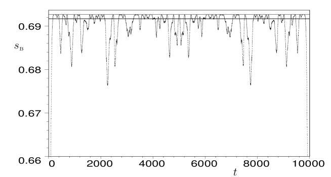
Figure 1: Half a cycle of the plot of $s_{{{\mbox{\tiny B}}}}$ against time, for a Kac ring of $10,000$ spins. There are $m=509$ spin-flippers, distributed randomly around the ring and the evolution is initiated in the low-entropy state $k=4993$. The upper and lower horizontal lines correspond respectively to $s_{{\mbox{\tiny B}}}(\mu_{{{\mbox{\tiny Max}}}})=0.69266408$ and $s_{{\mbox{\tiny B}}}(\mu_{221})=0.69168704$.

The putative equilibrium state, representing $99.999\%$ of $\Gamma_{10,000}$ is given by the region bounded by the horizontal lines in the figure. If the system were ergodic (like the baker’s gas) we would expect the system to spend almost all of the 10,000 time steps in this region, whereas in this particular simulation only 4658 steps satisfied this condition. This is to be expected as the Kac ring is not ergodic, but has an ergodic decomposition into cycles of which this figure represents half a cycle. The proportion of ‘equilibrium states’ will differ between cycles. So the problems with defining an equilibrium region are:

1. Just choosing the largest macrostate as the equilibrium region, does not guarantee that this region becomes an increasing proportion of phase space as $N$ increases. In fact the reverse is the case for the Kac ring.

2. Any choice of a collection of macrostates to represent equilibrium is:

   1. Arbitrary: leading to an arbitrary division between fluctuations within and out of equilibrium, as is shown in the profile in Fig. 1.

   2. Difficult: as we have shown in the Kac ring. Except for ergodic systems there is no clear way to make a choice which guarantees that the system will spend most of its time in equilibrium. The choice of a region consisting of $99.999\%$ of phase space still yields an evolution where only about $47\%$ of the points on the trajectory lie within it.

But why define equilibrium in this binary way? We suggest that the quality which we are trying to capture is a matter of degree, rather than the two-valued property of either being in equilibrium or not in equilibrium. We, therefore, make the following proposal:

Definition (C):All references to a system being, or not being, in equilibrium should be replaced by references to the commonness of the state of the system, with this property being measured by (some possibly-scaled form of) the Boltzmann entropy.

2.2 We Need Thermodynamic-Like Behaviour to beTypical

By this we mean that most initial states of the system should lead tothermodynamic-like behaviour. Before discussing the dynamic properties needed for this, we shall refer briefly to the more limited notion of typicality employed by the Neo-Boltzmannians and contained in the assertion (Lebowitz; 1999, S348) “that $S_{{{\mbox{\tiny B}}}}$ will typically be increasing in a way which explains and describes qualitatively the evolution towards equilibrium of macroscopic systems”. The conditions for this to be the case were first discussed by Ehrenfest and Ehrenfest-Afanassjewa (1912, 32–34).

Consider a macrostate $\mu$ divided into four parts $\mu^{(--)}$, $\mu^{(-+)}$, $\mu^{(+-)}$, $\mu^{(++)}$, where $\mu^{(-+)}$ consists of those points in $\mu$ which have evolved from a smaller macrostate and which evolve into a larger macrostate, with the other parts defined in a similar way. On grounds of symmetry, if $\boldsymbol{x}$ and $\mathfrak{I}\boldsymbol{x}$ are both in $\mu$, then ${\sf m}(\mu^{(-+)})={\sf m}(\mu^{(+-)})$; otherwise the macrostates will be in reversal pairs with plus and minus signs interchanged. In order for forward evolution to a larger macrostate to be typical it must be the case that the overwhelmingly largest part of $\mu$ is $\mu^{(++)}$. This was asserted without proof by Ehrenfest and Ehrenfest-Afanassjewa (1912, 33). More recent arguments have been advanced from the point of view that a macrostate is more likely to be surrounded by larger macrostates or that it is easier to ‘aim at’ a larger, rather than a smaller, neighbouring macrostate. Even accepting this argument, it can at the most explain how, if the state of a system is assigned randomly to a point in a macrostate, then the subsequent first transition is to a larger macrostate. As was pointed out by Lavis (2005), it gives no explanation for the entropy direction at the next transition, since the part of the macrostate occupied after the first transition will be determined by the dynamics. In any case, we wish to argue that this is a too narrowly defined version of typicality, which should be applied to thermodynamic-like behaviour over the whole evolution.

We have already argued in Sect. 2.1 that commonness or ‘equilibriumness’ is a matter of degree and it is clear that thermodynamic-like behaviour is also a matter of degree, for which we need to proposed a measure. A difference between these properties is that commoness is something which can be assessed at an instant of time, whereas thermodynamic-like behaviour is a temporally global property assessed over the whole trajectory.

Let ${\mathcal{L}}_{\boldsymbol{x}}$ be a trajectory in $\Gamma_{{{\mbox{\tiny$N$}}}}$ identified (uniquely) by the property that it passes through the point $\boldsymbol{x}$ and let ${\sf T}_{\boldsymbol{x}}(\gamma)$ be the proportion of time which the phase point evolving along ${\mathcal{L}}_{\boldsymbol{x}}$ spends in the some $\gamma\subset\Gamma_{{\mbox{\tiny$N$}}}$. Definition TL1 is an informal qualitative definition of thermodynamic-like behaviour, for which we need the entropy profile of $s_{{{\mbox{\tiny B}}}}$, not only to be quite close to $(s_{{{\mbox{\tiny B}}}})_{{\mbox{\tiny Max}}}:\!\mbox{$=$}\,s_{{{\mbox{\tiny B}}}}(\mu_{{\mbox{\tiny Max}}})$ for most of its evolution, but also for fluctuations around this value to be fairly small. We, therefore, propose the following definition:

Definition (TL2):The degree to which the evolution of the system is thermodynamic-like along ${\mathcal{L}}_{\boldsymbol{x}}$ is measured by the extent to which

$$\triangle_{\boldsymbol{x}}[s_{{{\mbox{\tiny B}}}}] :\!\mbox{$=$}\, |\langle s_{{{\mbox{\tiny B}}}}\rangle_{\boldsymbol{x}}-(s_{{{\mbox{\tiny B}}}})_{{{\mbox{\tiny Max}}}}|,$$

and

$$\Psi_{{\mbox{\tiny$N$}}}[s_{{{\mbox{\tiny B}}}}] :\!\mbox{$=$}\, \sqrt{\langle\left[s_{{{\mbox{\tiny B}}}}-\langle s_{{{\mbox{\tiny B}}}}\rangle_{\boldsymbol{x}}\right]^{2}\rangle_{\boldsymbol{x}}},$$ (7)

are small, where

$$\langle s_{{{\mbox{\tiny B}}}}\rangle_{\boldsymbol{x}}:\!\mbox{$=$}\,\sum_{\{\mu\}}{\sf T}_{\boldsymbol{x}}(\mu)s_{{{\mbox{\tiny B}}}}(\mu),$$ (8)

is the time-average of $s_{{{\mbox{\tiny B}}}}$ along ${\mathcal{L}}_{\boldsymbol{x}}$ and $\Psi_{\boldsymbol{x}}[s_{{{\mbox{\tiny B}}}}]$ is the standard deviation with respect to the time distribution.

Of course, it could be regarded as unsatisfactory that two parameters are used as a measure of the degree of a property and it is a matter of judgement which is more important. For the Kac ring of 10,000 spins with the entropy profile shown in Fig. 1,

$$\triangle_{\boldsymbol{x}}[s_{{{\mbox{\tiny B}}}}]=0.58122724\times 10^{-2},\hskip 19.91684pt\Psi_{\boldsymbol{x}}[s_{{{\mbox{\tiny B}}}}]=0.31802804\times 10^{-1}$$ (9)

and, as a comparison, for the same ring with the flippers placed at every tenth site

$$\triangle_{\boldsymbol{x}}[s_{{{\mbox{\tiny B}}}}]=0.20078055,\hskip 19.91684pt\Psi_{\boldsymbol{x}}[s_{{{\mbox{\tiny B}}}}]=0.20632198.$$ (10)

It is clear (and unsurprising) that the random distribution of spin flippers leads to more thermodynamic-like behaviour.

To explore the consequences of TL2 we distinguish between four aspects of a system:

1. The number of microsystems $N$ and their degrees of freedom, together giving the phase space $\Gamma_{{\mbox{\tiny$N$}}}$, with points representing microstates.

2. The measure ${\sf m}$ on $\Gamma_{{\mbox{\tiny$N$}}}$.

3. The mode of division of $\Gamma_{{\mbox{\tiny$N$}}}$ into the set $\{\mu\}$ of macrostates.

4. The ${\sf m}$-measure preserving dynamics of the system.

Having chosen (i) and (ii) the choices for (iii) and then (iv) are not unique. In the case of the baker’s gas (Lavis; 2005), $\Gamma_{{\mbox{\tiny$N$}}}$ is a $2N$–dimensional unit hypercube with volume measure. Macrostates are specified by partitioning each square face of the hypercube. With such a setup it would now be possible to choose all manner of discrete-time dynamics.

Whether a system is ergodic will be determined by (i), (ii) and (iv) and, if it is,

$${\sf T}_{\boldsymbol{x}}(\gamma)=\tau(\gamma),\hskip 19.91684pt\mbox{where}\hskip 19.91684pt\tau(\gamma):\!\mbox{$=$}\,\frac{{\sf m}(\gamma)}{{\sf m}(\Gamma_{{{\mbox{\tiny$N$}}}})},\hskip 28.45274pt\mbox{$\forall$\hskip 2.84544pt $\gamma\subset\Gamma_{{\mbox{\tiny$N$}}}$,}$$ (11)

is both the proportion of $\Gamma_{{\mbox{\tiny$N$}}}$ in $\gamma$ and of the time spent in $\gamma$, f.a.a. ${\mathcal{L}}_{\boldsymbol{x}}\in\Gamma_{{\mbox{\tiny$N$}}}$. This will be the case for the baker’s gas but not the Kac ring. For any specification of (i)–(iii) we denote the results of computing $\langle s_{{{\mbox{\tiny B}}}}\rangle_{\boldsymbol{x}}$, $\triangle_{\boldsymbol{x}}[s_{{{\mbox{\tiny B}}}}]$ and $\Psi_{\boldsymbol{x}}[s_{{{\mbox{\tiny B}}}}]$ using (11) by $\langle s_{{{\mbox{\tiny B}}}}\rangle$, $\triangle[s_{{{\mbox{\tiny B}}}}]$ and $\Psi[s_{{{\mbox{\tiny B}}}}]$; that is to say, we omit the unnecessary trajectory-identifying subscript $\boldsymbol{x}$. If we were able to devise a model with (i)–(iii) the same as the $N=10,000$ Kac ring, but with an ergodic dynamics, we would have

$$\begin{array}[]{l}\langle s_{{{\mbox{\tiny B}}}}\rangle=0.69261408,\\[7.11317pt] \triangle[s_{{{\mbox{\tiny B}}}}]=0.49997497\times 10^{-4},\hskip 19.91684pt\Psi[s_{{{\mbox{\tiny B}}}}]=0.70707142\times 10^{-4}\end{array}$$ (12)

and it is not difficult to show that $\triangle[s_{{{\mbox{\tiny B}}}}]$ and $\Psi[s_{{{\mbox{\tiny B}}}}]$ are monotonically decreasing functions of $N$. Ergodicity leads to more thermodynamic-like behaviour, which becomes increasingly thermodynamic-like with increasing $N$. This behaviour is also typical, since it occurs f.a.a. ${\mathcal{L}}_{\boldsymbol{x}}\in\Gamma_{{\mbox{\tiny$N$}}}$.

Of course, the results (12) are not simply dependent on the putative ergodic dynamics of the system, but also on the way that the macrostates have been defined. If the time average of $s_{{{\mbox{\tiny B}}}}(\boldsymbol{x})$ is to be close to $(s_{{{\mbox{\tiny B}}}})_{{\mbox{\tiny Max}}}$ and if the fluctuations in $s_{{{\mbox{\tiny B}}}}(\boldsymbol{x})$ are to be small then most of $\Gamma_{{\mbox{\tiny$N$}}}$ must lie in macrostates with $s_{{\mbox{\tiny B}}}(\mu)$ close to $(s_{{\mbox{\tiny B}}})_{{\mbox{\tiny Max}}}$. In the case of the Kac ring, with $N=10,000$, 99.98% of $\Gamma_{10000}$ lies in macrostates with $s_{{\mbox{\tiny B}}}(\mu)>0.999(s_{{\mbox{\tiny B}}})_{{\mbox{\tiny Max}}}$. However, of course, the Kac ring, although not ergodic, gives every appearance, at least in the instances investigated (see Fig. 1), of behaving in a thermodynamic-like manner. Although ergodicity, with a suitable macrostate structure, is sufficient for thermodynamic-like behaviour, it is clearly not necessary.

Consider the case where $\Gamma_{{{\mbox{\tiny$N$}}}}$ can be ergodically decomposed; meaning that

$$\Gamma_{{{\mbox{\tiny$N$}}}}=\displaystyle{\bigcup_{\{\alpha\}}}\,\Gamma_{\alpha},$$ (13)

where $\Gamma_{\alpha}$ is invariant and indecomposable under $\{\phi_{t}\}$. Then the time spent in $\gamma\subset\Gamma_{{\mbox{\tiny$N$}}}$ is

$${\sf T}_{\alpha}(\gamma)=\frac{{\sf m}(\gamma\cap\Gamma_{\alpha})}{{\sf m}(\Gamma_{\alpha})},\hskip 28.45274pt\mbox{f.a.a.}\hskip 14.22636pt{\mathcal{L}}_{\boldsymbol{x}}\in\Gamma_{\alpha},$$ (14)

and we, henceforth, identify a time average along a trajectory in $\Gamma_{\alpha}$ using $\langle\cdots\rangle_{\alpha}$ with $\alpha$ also replacing the subscript $\boldsymbol{x}$ in (2.2) and (7). In the case of the Kac ring the index $\alpha$ labels the cycles which form the ergodic decomposition of $\Gamma_{{\mbox{\tiny$N$}}}$. For a particular cycle, like that shown in Fig. 1, ${\sf T}_{\alpha}(\mu)$ is obtained simply by counting the number of times the phase point visits each macrostate in a complete cycle. The data are then used to compute the results given in (9). A plot of ${\sf T}_{\alpha}(\mu_{k})$ against the microstate index $k$ is shown in Fig. 2 with a comparison made with $\tau(\mu_{k})$, the corresponding curve for a system with ergodic dynamics. This gives a graphic illustration of the suggestion that

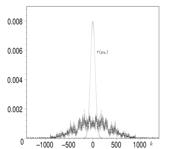
Figure 2: Plot of ${\sf T}_{\alpha}(\mu_{k})$ for the cycle $\alpha$ of the Kac ring shown in Fig. 1 together with the corresponding curve of $\tau(\mu_{k})$ for a system with ergodic dynamics.

ergodic systems, with a suitable choice of macrostates, are likely to be more thermodynamic-like in their behaviour than non-ergodic systems. It might also be speculated that $\varepsilon$–ergodic systems (Vranas; 1998) show increasingly thermodynamic-like behaviour with decreasing $\varepsilon$.

Another advantage of an ergodic system is that, f.a.a. ${\mathcal{L}}_{\boldsymbol{x}}\in\Gamma_{{\mbox{\tiny$N$}}}$, the level of thermodynamic-like behaviour will be the same. This contrasts with an ergodic decomposition characterized by (13), where it is possible for differing levels of thermodynamic-like behaviour to be exhibited within different members of the decomposition. To be precise, take small positive $\varepsilon_{\triangle}$ and $\varepsilon_{\Psi}$ and regard behaviour along a trajectory as thermodynamic-like if and only if both $\triangle_{\alpha}[s_{{{\mbox{\tiny B}}}}]<\varepsilon_{\triangle}$ and $\Psi_{\alpha}[s_{{{\mbox{\tiny B}}}}]<\varepsilon_{\Psi}$. Let $\Gamma^{({{\mbox{\tiny T}}})}_{{\mbox{\tiny$N$}}}$ be the union of all $\Gamma_{\alpha}$ in which the behaviour is thermodynamic-like with $\Gamma^{({{\mbox{\tiny A}}})}_{{\mbox{\tiny$N$}}}=\Gamma_{{\mbox{\tiny$N$}}}\backslash\Gamma^{({{\mbox{\tiny T}}})}_{{\mbox{\tiny$N$}}}$.

In the discussion of the Boltzmann approach we have so far avoided any reference to probabilities. To complete the discussion in this section and to relate our arguments to the Gibbs approach we shall need (see Lavis; 2005) to introduce two sets of probabilities for a system with the ergodic decomposition (13). The first of these is ${\sf p}_{\alpha}:\!\mbox{$=$}\,{\sf Prob}(\boldsymbol{x}\in\Lambda_{\alpha})$, $\forall$ $\Gamma_{\alpha}$. Then thermodynamic-like behaviour will be typical for the system if

$$\sum_{\Gamma_{\alpha}\subset\Gamma^{({{\mbox{\tiny A}}})}}{\sf p}_{\alpha}\ll 1.$$ (15)

Thus we have two levels of degree, the first represented by the choices of $\varepsilon_{\triangle}$ and $\varepsilon_{\Psi}$ and the second concerning the extent to which (15) is satisfied.

3 Reconciling Gibbs and Boltzmann

As we saw in Sect. 1, the Gibbs approach depends on defining a probability density function $\rho(\boldsymbol{x})$ on $\Gamma_{{\mbox{\tiny$N$}}}$, for a system ‘at equilibrium’. Thus we must address more directly the question of probabilities. Assuming the ergodic decomposition (13), we take the time-average definition of Von Plato (1989), for which

$${\sf Prob}(\boldsymbol{x}\in\gamma|\boldsymbol{x}\in\Gamma_{\alpha}):\!\mbox{$=$}\,{\sf T}_{\alpha}(\gamma),\hskip 19.91684pt\mbox{$\forall$ $\gamma\subset\Gamma_{{\mbox{\tiny$N$}}}$,}$$ (16)

where ${\sf T}_{\alpha}(\gamma)$ is given by (14). Thus the probability density function for $\Gamma_{\alpha}$ is

$$\rho_{\alpha}(\boldsymbol{x})=\left\{\begin{array}[]{ll}1/{\sf m}(\Gamma_{\alpha}),&\mbox{$\boldsymbol{x}\in\Gamma_{\alpha},$}\\[7.11317pt] 0,&\mbox{otherwise,}\end{array}\right.$$ (17)

from which we have

$$\rho(\boldsymbol{x})=\stackrel{{\scriptstyle{{\mbox{\tiny E}}}{{\mbox{\tiny D}}}}}{{\overline{\rho_{\alpha}(\boldsymbol{x})}}}\,\,:\!\mbox{$=$}\,\sum_{\{\alpha\}}\rho_{\alpha}(\boldsymbol{x}){\sf p}_{\alpha}.$$ (18)

If we assume that all points of $\Gamma_{{\mbox{\tiny$N$}}}$ are equally likely, then on Bayesian/Laplacean grounds, and consonant with the approach of Bricmont (2001), we should choose

$${\sf p}_{\alpha}={\sf m}(\Gamma_{\alpha})/{\sf m}(\Gamma_{{\mbox{\tiny$N$}}}),$$ (19)

giving, from (18), $\rho(\boldsymbol{x})=1/{\sf m}(\Gamma_{{\mbox{\tiny$N$}}})$, which is the microcanonical distribution and for which, from (1),

$$s_{{\mbox{\tiny G}}}:\!\mbox{$=$}\,S_{{\mbox{\tiny G}}}/(Nk_{{\mbox{\tiny B}}})=\ln[{\sf m}(\Gamma_{{\mbox{\tiny$N$}}})]=s_{{\mbox{\tiny B}}}(\Gamma_{{\mbox{\tiny$N$}}}).$$ (20)

It also follows, from (2), (8), (11) and (19) that

$$\stackrel{{\scriptstyle{{\mbox{\tiny E}}}{{\mbox{\tiny D}}}}}{{\overline{\langle s_{{\mbox{\tiny B}}}\rangle_{\alpha}}}}=\langle s_{{\mbox{\tiny B}}}\rangle.$$ (21)

Lavis (2005) has proposed a general scheme for relating a phase function $f$, defined on $\boldsymbol{x}\in\Gamma_{{\mbox{\tiny$N$}}}$ to a macro-function $\mathscr{F}$ defined on the macrostates $\{\mu\}$ and then to a thermodynamic function $F$. The first step is to course grain $f(\boldsymbol{x})$ over the macrostates to produce $\mathscr{F}(\mu)$. The second step is to define the thermodynamic variable $F$ along the trajectory ${\mathcal{L}}_{\boldsymbol{x}}$ as $\langle\mathscr{F}\rangle_{\boldsymbol{x}}$. In the case of the Boltzmann entropy, which is both a phase function and a macro-function the first step in this procedure is unnecessary since it already, by definition, course grained over the macrostates. Then we proceed to identify the dimensionless thermodynamic entropy per microsystem with $\langle s_{{\mbox{\tiny B}}}\rangle_{\boldsymbol{x}}$. In the case of a system with an ergodic decomposition this definition would yield a different thermodynamic entropy $s_{\alpha}$ for each member of the decomposition, with, from (2.2),

$$s_{\alpha}:\!\mbox{$=$}\,\langle s_{{\mbox{\tiny B}}}\rangle_{\alpha}=(s_{{\mbox{\tiny B}}})_{{\mbox{\tiny Max}}}-\triangle_{\alpha}[s_{{\mbox{\tiny B}}}].$$ (22)

In the case where the behavior is thermodynamic-like in $\Gamma_{\alpha}$, $s_{\alpha}$ differs from $(s_{{\mbox{\tiny B}}})_{{\mbox{\tiny Max}}}$ by at most some small $\varepsilon_{\triangle}$ and, if (15) holds, this will be the case for measurements along most trajectories. In the case of the Kac ring with $N=10,000$ and the trajectory investigated for Figs. 1 and 2 the actual difference is given in (9), a value which is likely to decrease with increasing $N$.

It is often said that in “equilibrium [the Gibbs entropy] agrees with Boltzmann and Clausius entropies (up to terms that are negligible when the number of particles is large) and everything is fine” (Bricmont; 1995, 188). Interpreted within the present context this means that the good approximation $s_{{\mbox{\tiny B}}}(\mu_{{\mbox{\tiny Max}}})$, for the entropy per microsystem of a system for which thermodynamic-like behaviour is typical, can be replace by $s_{{\mbox{\tiny G}}}=s_{{\mbox{\tiny B}}}(\Gamma_{{\mbox{\tiny$N$}}})$. The advantage of this substitution is obvious, since the first expression is dependent on the division into macrostates and second is not. However a little care is needed in justifying this substitution. It is not valid because, as asserted in the quote from Bricmont on page 2.1, $\mu_{{\mbox{\tiny Max}}}$ occupies an increasing proportion of $\Gamma_{{\mbox{\tiny$N$}}}$ as $N$ increases. Indeed, we have shown for the Kac ring the reverse is the case. That proportion becomes vanishingly small as $N$ increases. However, the required substitution can still be made, since for that model

$$\frac{s_{{\mbox{\tiny B}}}(\mu_{{\mbox{\tiny Max}}})}{s_{{\mbox{\tiny B}}}(\Gamma_{{\mbox{\tiny$N$}}})}\simeq 1-\frac{\ln(N)}{2N\ln(2)},\hskip 28.45274pt\mbox{as $N\rightarrow\infty$.}$$ (23)

Although it may seem that the incorrect intuition on the part of Bricmont et al. concerning the growth in the relative size of the largest macrostate, leading as it does to the correct conclusion with respect to entropy, is easily modified and of no importance, we have shown in Sect. 2.1 that it has profound consequences for the attempt to define equilibrium in the Boltzmann approach.

It should be emphasized that the Gibbs entropy (20) is no longer taken as that of some (we would argue) non-existent equilibrium state, but as an approximation to the true thermodynamic entropy which is the time-average over macrostates of the Boltzmann entropy. The use of a time-independent probability density function for the Gibbs entropy is not because the system is at equilibrium but because the underlying dynamics is autonomous. The thermodynamic entropy approximated by the Gibbs entropy (20) remains constant if the phase space remains unchanged but changes discontinuously if a change in external constraints leads to a change in $\Gamma_{{\mbox{\tiny$N$}}}$. An example of this, for a perfect gas in a box when a partition is removed, is considered by Lavis (2005) who shows that the Boltzmann entropy follows closely the step change in the Gibbs entropy.

4 Conclusions

In our programme for reconciling the Boltzmann and Gibbs approaches to statistical mechanics we have made use both of ergodicity and ergodic decomposition and there is deep (and justified) suspicion of the use of ergodic arguments, particularly among philosophers of physics. Earman and Rédei (1996, 75) argue “that ergodic theory in its traditional form is unlikely to play more than a cameo role in whatever the final explanation of the success of equilibrium statistical mechanics turns out to be”. In its ‘traditional form’ the ergodic argument goes something like this: (a) Measurement processes on thermodynamic systems take a long time compared to the time for microscopic processes in the system and thus can be effectively regarded as infinite time averages. (b) In an ergodic system the infinite time average can be shown, for all but a set of measure zero, to be equal to the macrostate average with respect to an invariant normalized measure which is unique. The traditional objections to this argument are also well known: (i) Measurements may be regarded as time averages, but they are not infinite time averages. If they were one could not, by measurement, investigate a system not in equilibrium. In fact, traditional ergodic theory does not distinguish between systems in equilibrium and not in equilibrium. (ii) Ergodic results are all to within sets of measure zero and one cannot equate such sets with events with zero probability of occurrence. (iii) Rather few systems have been shown to be ergodic. So one must look for a reason for the success of equilibrium statistical mechanics for non-ergodic systems and when it is found it will make the ergodicity of ergodic systems irrelevant as well.

Our use of ergodicity differs substantially from that described above and it thus escapes wholly or partly the strictures applied to it. In respect of the question of equilibrium/non-equilibrium we argue that the reason this does not arise in ergodic arguments is that equilibrium does not exist. The phase point of the system, in its passage along a trajectory, passes through common (high entropy) and uncommon (low entropy) macrostates and that is all. So we cannot be charged with ‘blurring out’ the period when the system was not in equilibrium. The charge against ergodic arguments related to sets of measure zero is applicable only if one wants to argue that the procedure always works; that is that non-thermodynamic-like behaviour never occurs. But we have, in this respect taken a Boltzmann view. We need thermodynamic-like behaviour to be typical and we have proposed conditions for this to be the case. But we admit the possibility of atypical behaviour occurring with small but not-vanishing probability. While the class of systems admitting a finite or denumerable ergodic decomposition is likely to be much larger than that of the purely ergodic systems, there remains the difficult question of determining general conditions under which the temporal behaviour along a trajectory, measured in terms of visiting-times in macrostates, approximates, in most members of the ergodic decomposition, to thermodynamic-like behaviour.

References

- (1)
- Birkhoff (1931) Birkhoff, Garrett D. (1931), Proof of the ergodic theorem, Proc. Natl. Ac. Sci. USA 17: 656–660.
- Bishop (2004) Bishop, Robert C. (2004), Nonequilibrium statistical mechanics Brussels–Austin style, Stud. Hist. Phil. Phys. 35: 1–30.
- Bricmont (1995) Bricmont, Jean (1995), Science of chaos or chaos in science?, Physicalia 17: 159–208.
- Bricmont (2001) Bricmont, Jean (2001), Bayes, Boltzmann and Bohm: probabilities in physics, in J. Bricmont, D. Dürr, M. C. Galvotti, G. Ghirardi, F. Petruccione and N. Zanghi (eds), Chance in Physics: Foundations and Perspectives, Springer, 3–21.
- Earman and Rédei (1996) Earman, John and Miklós Rédei, (1996), Why ergodic theory does not explain the success of equilibrium statistical mechanics, Brit. J. Phil. Sci. 47: 63–78.
- Ehrenfest and Ehrenfest-Afanassjewa (1912) Ehrenfest, Paul and Tatiana Ehrenfest-Afanassjewa, (1912), The Conceptual Foundations of the Statistical Approach in Mechanics, English translation, Cornell University Press.
- Goldstein (2001) Goldstein, Sheldon (2001), Boltzmann’s approach to statistical mechanics, in J. Bricmont, D. Dürr, M. C. Galvotti, G. Ghirardi, F. Petruccione and N. Zanghi (eds), Chance in Physics: Foundations and Perspectives, Springer, 39–54.
- Kac (1959) Kac, Mark (1959), Probability and Related Topics in the Physical Sciences, Interscience.
- Lavis (1977) Lavis, David A. (1977), The role of statistical mechanics in classical physics, Brit. J. Phil. Sci. 28: 255–279.
- Lavis (2005) Lavis, David A. (2005), Boltzmann and Gibbs: An attempted reconciliation, Stud. Hist. Phil. Mod. Phys. 36: 245–273.
- Lebowitz (1993) Lebowitz, Joel L. (1993), Boltzmann’s entropy and time’s arrow, Physics Today 46: 32–38.
- Lebowitz (1999) Lebowitz, Joel L. (1999), Statistical mechanics: A selective review of two central issues, Rev. Mod. Phys. 71: S346–S357.
- Prigogine (1994) Prigogine, Ilya (1994), Les Lois du Chaos, Flammarion.
- Von Plato (1989) Von Plato, Jan (1989), Probability in dynamical systems, in J. E. Fenstad, I. T. Frolov and R. Hilpinen (eds), Logic, Methodology and Philosophy of Science VIII, Elsevier, 427–443.
- Vranas (1998) Vranas, Peter B. M. (1998), Epsilon-ergodicity and the success of equilibrium statistical mechanics, Philosophy of Science 65: 688–708.