Cutoff effects for Wilson twisted mass fermions at tree-level of perturbation theory

Abstract:

We study cutoff effects at tree-level of perturbation theory for standard Wilson and Wilson twisted mass fermionic lattice actions with $N_{f}=2$ flavour degenerate quarks. The discretization effects are investigated by computing the mass spectrum and decay amplitudes for different hadron interpolating fields and the scaling behaviour towards the continuum limit is analyzed. It is shown that the Wilson and the mass average methods are equivalent and lead to $O(a)$ improved $\mathcal{R}_{5}$-parity even lattice observables. We also demonstrate that automatic $O(a)$ improvement works in case of Wilson twisted mass fermions at maximal twist and that this improvement is realized even if the condition of maximal twist is achieved only up to $O(a)$ cutoff effects. We demonstrate that in the chiral limit standard Wilson fermions show scaling violations of $O(a^{2})$ while for maximally twisted mass fermions these violations are only of $O(a^{4})$. For our analytical calculations, lattices with sizes $L=aN$ and periodic boundary conditions in the spatial directions have been chosen while infinite extension in the time direction, $L_{4}=\infty$, is considered.

1 Introduction: Wilson twisted mass action

In this contribution, we study the cutoff effects of observables computed on a lattice with lattice spacing $a$ when Wilson twisted mass fermions at maximal twist are considered . The twisted mass QCD action in the continuum, at tree-level of perturbation theory, is given by

$$S_{F}^{tm}[\chi,\bar{\chi}]=\int\,d^{4}x\,\bar{\chi}(x)\,(\gamma_{\mu}\partial_{\mu}+m_{0}+i\mu_{q}\gamma_{5}\tau^{3})\,\chi(x),$$ (1)

with $\tau^{3}$ the third Pauli matrix acting in flavour space and $\{\chi,\bar{\chi}\}$ the so-called twisted basis. In equation (1), $m_{0}$ denotes the bare untwisted quark mass and $\mu_{q}$ the bare twisted quark mass. The mass term can be written in terms of a polar mass $M$ and a polar angle $\alpha$ as

$$m_{0}+i\mu_{q}\gamma_{5}\tau^{3}=M\,e^{i\alpha\gamma_{5}\tau^{3}}\qquad\text{with}\qquad M=\sqrt{m_{0}^{2}+\mu_{q}^{2}}\,,\quad\alpha=\arctan(\frac{\mu_{q}}{m_{0}}).$$ (2)

The twisted basis $\{\chi,\bar{\chi}\}$ is related to the so-called physical basis $\{\psi,\bar{\psi}\}$ by the non-anomalous axial transformation

$$\psi(x)=e^{i\omega\gamma_{5}\frac{\tau^{3}}{2}}\chi(x)\qquad\bar{\psi}(x)=\bar{\chi}(x)e^{i\omega\gamma_{5}\frac{\tau^{3}}{2}}\;,$$ (3)

for the particular choice of the twisting angle $\omega=\alpha$, since it brings the twisted mass QCD action back to the standard form. The Wilson-regularized twisted mass action (Wtm) written in the twisted basis has the form

$$S_{F}^{Wtm}[\chi,\bar{\chi}]=a^{4}\sum_{x}\,\bar{\chi}(x)\,[D_{W}+m_{0}+i\mu_{q}\gamma_{5}\tau^{3}]\,\chi(x)\,;\quad D_{W}=\frac{1}{2}\{\gamma_{\mu}(\partial_{\mu}+\partial_{\mu}^{*})-ar\partial_{\mu}^{*}\partial_{\mu}\}$$ (4)

with $D_{W}$ the Wilson-Dirac operator of the free case, $\partial_{\mu}$ and $\partial_{\mu}^{*}$ the forward and backward partial lattice derivatives and $-\frac{ar}{2}\partial_{\mu}^{*}\partial_{\mu}$ the Wilson term.

2 Wilson twisted mass free-fermion propagator with infinite time-extent lattices

The expression for the Wilson twisted mass fermion propagator in the twisted basis, at tree-level of perturbation theory (PT) and in momentum space is given by

$$\widetilde{S}(p)=\frac{-i\frac{1}{a}\sin(ap_{4})\gamma^{4}\mathbbm{1}_{f}-i\mathcal{K}\mathbbm{1}_{f}+\bigl{[}\frac{r}{a}\left(1-\cos(ap_{4})\right)+\mathcal{M}\bigr{]}\mathbbm{1}\mathbbm{1}_{f}-i\mu_{q}\,\gamma^{5}\tau^{3}}{\frac{1}{a^{2}}\sin^{2}(ap_{4})+\mathcal{K}^{2}+\bigl{[}\frac{r}{a}\left(1-\cos(ap_{4})\right)+\mathcal{M}\bigr{]}^{2}+\mu_{q}^{2}},$$ (5)

where $\mathbbm{1}$ and $\mathbbm{1}_{f}$ are the identity matrices in Dirac and flavour space. The structure in colour space has not been written since it is just an identity matrix at tree level of PT and we have defined,

$$\mathcal{M}(p)=m_{0}+\frac{2r}{a}\sum_{i=1}^{3}\,\sin^{2}(\frac{ap_{i}}{2}),\qquad\mathcal{K}=\frac{1}{a}\sum_{i=1}^{3}\,\gamma^{i}\sin(ap_{i}).$$ (6)

We obtain the expression for the quark propagator in the time-momentum representation when an infinite extension of the time direction is considered. To perform the integral in the continuous momentum $p_{4}$ amounts to performing a contour integral and compute the residues of the integrand. The integration contour encloses the poles of the integrand at the energy points

$$\left\{\begin{array}[]{lll}p_{4}=\frac{1}{a}iE_{1}&\cosh E_{1}=\frac{\mathcal{U}-r\left(r+a\mathcal{M}\right)}{1-r^{2}}&\text{physical pole}\\ p_{4}=\frac{1}{a}(\pi+iE_{2})&\cosh E_{2}=\frac{\mathcal{U}+r\left(r+a\mathcal{M}\right)}{1-r^{2}}&\text{doubler pole}\end{array}\right.$$

with $\mathcal{U}^{2}=\left(1+ar\mathcal{M}\right)^{2}+\left(1-r^{2}\right)\left(a^{2}\mathcal{K}^{2}+a^{2}\mathcal{M}^{2}+a^{2}\mu_{q}^{2}\right)$. The final expression for the propagator, in the limit $r\rightarrow 1$, is then,

$$\begin{split}S_{\infty}\bigl{(}\vec{p},t\bigr{)}=\frac{1}{2\,\mathcal{U}\sinh E_{1}}&\Bigl{\{}\text{sgn}(t)\sinh E_{1}\gamma_{4}\mathbbm{1}_{f}-ia\mathcal{K}\mathbbm{1}_{f}+\bigl{[}\left(1-\cosh E_{1}\right)+a\mathcal{M}\bigr{]}\mathbbm{1}\mathbbm{1}_{f}\\ &-ia\mu_{q}\gamma_{5}\,\tau^{3}\Bigr{\}}e^{-E_{1}|\frac{t}{a}|}\>+\>\delta_{\frac{t}{a},0}\,\frac{1}{2\,(1+a\mathcal{M})}\mathbbm{1}\mathbbm{1}_{f}\end{split}$$ (7)

where $\cosh E_{1}=1+\frac{a^{2}\mathcal{K}^{2}+a^{2}\mathcal{M}^{2}+a^{2}\mu_{q}^{2}}{2\,(1+a\mathcal{M})}$.

The fermion propagator is a matrix in Dirac space and can hence be decomposed in terms of the Dirac gamma matrices as $S_{\infty}\bigl{(}\vec{p},t\bigr{)}=S_{U}\bigl{(}\vec{p},t\bigr{)}\,\mathbbm{1}+\sum_{\mu}\,S_{\mu}\bigl{(}\vec{p},t\bigr{)}\,\gamma_{\mu}+S_{5}\bigl{(}\vec{p},t\bigr{)}\,\gamma_{5}$.

3 Hadron correlation functions

3.1 Pseudo-scalar meson

The interpolating fields describing the charged pions, $\pi^{+}$ and $\pi^{-}$ respectively, in the physical and the twisted bases are

$$\mathcal{P}^{\pm}(x)\equiv\mathcal{P}^{1}(x)\mp i\mathcal{P}^{2}(x)=P^{1}(x)\mp iP^{2}(x)$$ (8)

where $\mathcal{P}^{a}(x)=\bar{\psi}(x)\gamma_{5}\frac{\tau^{a}}{2}\psi(x)$, with $a=1,2,3$, is the pseudo-scalar density written in the physical basis while $P^{a}(x)=\bar{\chi}(x)\gamma_{5}\frac{\tau^{a}}{2}\chi(x)$ is the pseudo-scalar density written in the twisted basis.

The time dependence of the two-point correlation function for the charged pseudo-scalar meson in the time-momentum representation is given by

$$C_{\mathcal{P}^{\pm}\mathcal{P}^{\pm}}(t)=\frac{N_{c}\,N_{d}}{L^{3}}\sum_{\vec{p}}\Bigl{\{}|S^{u}_{U}(\vec{p},t)|^{2}+\sum_{\mu=1}^{4}\>|S^{u}_{\mu}(\vec{p},t)|^{2}+|S^{u}_{5}(\vec{p},t)|^{2}\Bigr{\}}.$$ (9)

We denote the Wilson twisted mass fermion propagator in the twisted basis for “$u$ quarks” as $S^{u}$. Note that this is not identical in the twisted mass case with the propagator for “$d$ quarks” denoted as $S^{d}$. $N_{c}$ ($N_{d}$) is the number of colours (Dirac components).

3.2 Proton

The local interpolating field describing the proton in both bases is given by ,

$$\mathscr{P}_{\alpha}(x)\equiv-\sqrt{2}\epsilon_{abc}\bigl{[}\bar{\hat{d}}_{a}^{T}(x)\,C^{-1}\gamma_{5}\hat{u}_{b}(x)\bigr{]}\,\hat{u}_{\alpha,c}(x)=\sqrt{2}\,\epsilon_{abc}\,\bigl{[}d_{a}^{T}(x)\,C^{-1}\gamma_{5}\,u_{b}(x)\bigr{]}\,e^{i\frac{\omega}{2}\gamma_{5}}\,u_{\alpha,c}(x).$$ (10)

The expression for the time dependence of the proton correlation function is then

$$C_{\mathscr{P}\bar{\mathscr{P}}}(t)=\frac{N_{c}N_{d}}{L^{6}}\,\sum_{\vec{p}}\sum_{\vec{q}}\Bigl{\{}\cos(\omega)\,L_{U}(\vec{p},\vec{q},t)+L_{4}(\vec{p},\vec{q},t)+i\sin(\omega)L_{5}(\vec{p},\vec{q},t)\Bigr{\}},$$ (11)

with the definitions

$$\begin{split}L_{U,5}(\vec{p},\vec{q},t)\equiv S^{u}_{U,5}(-(\vec{p}+\vec{q}),t)\Bigl{\{}&(N_{d}+1)\,S^{u}_{U}(\vec{p},t)S^{u}_{U}(\vec{q},t)+(N_{d}+3)\,\sum_{\mu=1}^{4}\,S^{u}_{\mu}(\vec{p},t)S^{u}_{\mu}(\vec{q},t)\\ &-(N_{d}+1)\,S^{u}_{5}(\vec{p},t)S^{u}_{5}(\vec{q},t)\Bigr{\}}\end{split}$$ (12)

$$\begin{split}L_{\mu}(\vec{p},\vec{q},t)\equiv S^{u}_{\mu}(-(\vec{p}+\vec{q}),t)\Bigl{\{}&(N_{d}+3)\,S^{u}_{U}(\vec{p},t)S^{u}_{U}(\vec{q},t)+(N_{d}+1)\,\sum_{\mu=1}^{4}\,S^{u}_{\mu}(\vec{p},t)S^{u}_{\mu}(\vec{q},t)\\ &-(N_{d}+3)\,S^{u}_{5}(\vec{p},t)S^{u}_{5}(\vec{q},t)\Bigr{\}}.\end{split}$$ (13)

4 Scaling test

4.1 Wilson average (WA) and mass average (MA) for standard Wilson fermions

In Ref. [3] it has been demonstrated that when averaging physical observables computed with Wilson actions having opposite signs of the quark mass (MA) or opposite signs of the Wilson parameter (WA), these quantities are $O(a)$ improved. Since WA and MA are equivalent, we show in Figure 1, only the cutoff effects at the example of the proton mass when the MA is performed. In the left graph the behaviour of the proton mass $NM_{P}$ as a function of $\frac{1}{N}$ is given when a standard Wilson regularization is used. In order to describe the behaviour of the physical quantities computed analytically at selected values of $\frac{1}{N}$, we use the following fitting functions:

$$y_{1}=a_{0}+a_{1}\frac{1}{N}+a_{2}\frac{1}{N^{2}}\qquad y_{2}=b_{0}+b_{1}\frac{1}{N^{2}}+b_{2}\frac{1}{N^{4}}.$$ (14)

Here $y_{1}$ ($y_{2}$) is the physical observable under consideration and its value in the continuum limit is given by the coefficient $a_{0}$ ($b_{0}$). We use two functional forms, the first formula of equation (14) for a leading $\frac{1}{N}$ behaviour (standard Wilson fermions) and the second formula for $O(a)$-improved quantities.

The two lines in the left graph of Figure 1 originate from a fit to equation (14) and correspond to the proton mass obtained from the same Wilson actions differing only in the sign of the quark mass. The linear behaviour in $\frac{1}{N}$ shows the $O(a)$ scaling violations present in the standard Wilson theory. From the plot it is clear that in both cases the value of the proton mass in the continuum limit is the same and the expected one at tree-level of PT. From the fit, the corresponding coefficients $a_{1}$ turn out to be the same in magnitude but have opposite signs for positive and negative quark masses. Thus, performing the (MA), it is to be expected that the $O(a)$ effects cancel and the scaling behaviour changes drastically from a $\frac{1}{N}$ to a $\frac{1}{N^{2}}$ behaviour. This can indeed be seen in the right graph of Figure 1. Inspecting the fit coefficients $a_{2}$ and $b_{1}$, we find $a_{2}^{sW}\approx b_{1}^{MA}\approx 0.5$. Therefore, the magnitude of the leading order cutoff effects does not only change from an $O(a)$ to an $O(a^{2})$ behaviour but also the $O(a^{2})$ do not increase on performing the Wilson average with respect to the standard case.

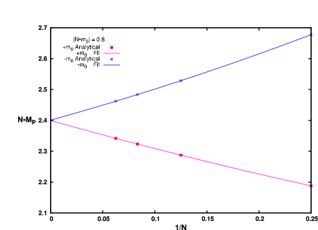
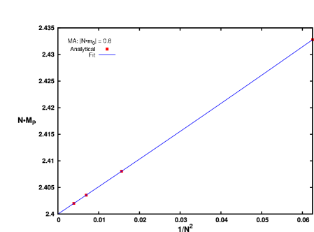
Figure 1: In the left graph, the cutoff effects and the continuum limit of the proton mass obtained from two standard Wilson actions differing only in the sign of the quark mass, $|Nm_{0}|=0.8$ are shown. The lattices are $4\leq N\leq 20$. In the right graph, the average of the proton masses obtained from the same two standard Wilson regularizations with quark masses $Nm_{0}=\pm 0.8$ (MA) has been calculated.

4.2 Wilson twisted mass fermions at maximal twist

Instead of performing a MA or WA, a way to obtain an automatic $O(a)$ improvement is to work with Wtm fermions at maximal twist [3]. Maximal twist is reached for a value of the twist angle of $\omega=\pi/2$. At tree-level of perturbation theory this can be achieved by simply setting the untwisted quark mass $m_{0}=0$. The value of the quark mass is now fully given by the twisted quark mass, $NM=N\mu_{q}$. The proton mass as a function of $\frac{1}{N^{2}}$ is shown in Figure 2 and the corresponding fit is performed using the second fitting function of equation (14). The figure clearly demonstrates that automatic $O(a)$ improvement is indeed working and that the cutoff effects have changed from a $\frac{1}{N}$ behaviour of standard Wilson fermions to a $\frac{1}{N^{2}}$ behaviour when maximally twisted mass Wilson fermions are employed. Moreover, as a result of the fit, the coefficient $b_{1}$ comes out to be very small, $b_{1}^{tm}=O(10^{-2})$. This value is one order of magnitude smaller than the corresponding coefficient $a_{2}$ of the $O(a^{2})$ effects for standard Wilson fermions which we find to be $a_{2}^{sW}=O(10^{-1})$. Note the the value of $b_{1}$ is also smaller than the one for the case of MA discussed above.

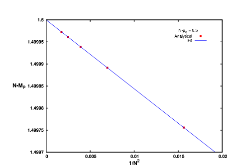
Figure 2: Cutoff effects in the proton mass with Wtm fermions at maximal twist. To study the case of maximal twist, we set the quark mass to $N\mu_{q}=0.5$. The lattices considered are taken as $4\leq N\leq 24$.

We have also analyzed the chiral limit behaviour of the pion and proton masses by determining the coefficients $a_{1}$ and $b_{1}$ of equations (14). In the case of standard Wilson fermions, the coefficient $a_{1}$ which determines the size of the $O(a)$ cutoff effects vanishes in the chiral limit thus leading to only $O(a^{2})$ scaling violations in the massless theory. For Wtm fermions at maximal twist the situation is even better. Here, the coefficient of the $O(a^{2})$ cutoff effects vanishes in the chiral limit, thus leading to scaling violations of $O(a^{4})$ only since all odd powers of $a$ vanish for maximally twisted mass fermions. Therefore, for Wilson twisted mass fermions at maximal twist the breaking of chiral symmetry at finite lattice spacing is much smaller than for standard Wilson fermions and maximally twisted mass fermions are indeed chirally improved.

4.2.1 Out of maximal twist

Here we want to study a situation when we allow an $O(a)$ error in setting the untwisted quark mass to zero. In order to realize this situation at tree-level of PT we ‘force’ these effects by simply fixing the twisted mass to be the physical quark mass and the untwisted mass is set to be proportional to $\frac{1}{N}$, as $N\mu_{q}=\alpha$ and $Nm_{0}=\frac{\beta}{N}\backsim O(a)$ where $\alpha$ is kept fixed and $\beta$ is a measure parametrizing the amount of violation of the maximal twist setup. The twist angle $\omega$ and the bare polar mass $M$ can be obtained as a function of $\alpha$ and $\beta$ as

$$\omega=\frac{\pi}{2}-\Bigl{(}\frac{\beta}{\alpha}\Bigr{)}\frac{1}{N}+O(\frac{1}{N^{2}}),\qquad NM=\alpha\Bigl{[}1+\frac{1}{2}\Bigl{(}\frac{\beta}{\alpha}\Bigr{)}^{2}\frac{1}{N^{2}}+O(\frac{1}{N^{4}})\Bigr{]}.$$ (15)

Therefore, even if the condition of maximal twist can be only obtained up to $O(a)$ cutoff effects, which is generically the case in practical numerical simulations, the observables, which are only functions of the polar mass, are still automatically $O(a)$ improved.

Moreover, equation (15) also shows how the size of the leading discretization effects depends on the ratio between the untwisted and twisted quark masses. This ratio in turn determines the value of the lattice spacing at which the asymptotic $\frac{1}{N^{2}}$ scaling sets in. Only when this ratio is small enough and hence the lattice does not need to be chosen too large a reliable continuum limit using reasonably sized lattices can be performed. The left graph of Figure 3 demonstrates that the asymptotic scaling sets in for lattices with $4\leq N\leq 64$ when $0\lesssim\frac{\beta}{\alpha}\lesssim 2$.

However, for $\frac{\beta}{\alpha}\,\gtrsim 10$ the continuum limit is not reliable anymore if $N$ is chosen to be too small. This can be seen in the right graph of Figure 3. Using only small values of $N$ leads to an inconsistent continuum limit value. Therefore, larger lattices are needed in order to obtain the correct continuum behaviour as can be also seen in the right graph of Figure 3. Here we have added a fit of the data for a value of $\beta=10.0$ taking only large lattices into account, i.e. using only values of $N\geq 40$. In this case, indeed the right continuum value is obtained. Of course, for practical simulations, using only lattices with $N\gg 40$ appears to be rather unrealistic.

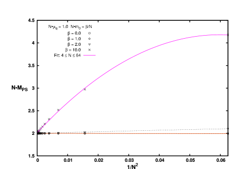
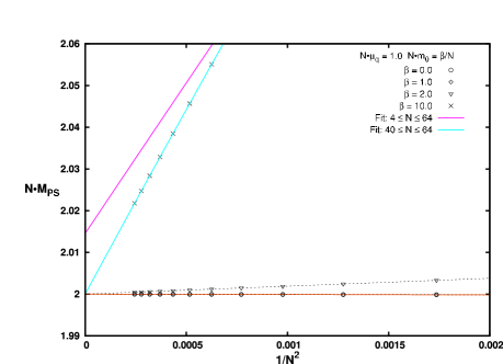
Figure 3: Left graph: Behaviour of the pion mass as a function of $\frac{1}{N^{2}}$, for lattices with size $4\leq N\leq 64$. The twisted quark mass is set to $N\mu_{q}=1.0$ and the untwisted quark mass is zero up to $O(a)$ cutoff effects i.e. $Nm_{0}=\frac{\beta}{N}$ with $\beta=0.0,1.0,2.0,10.0$. Right graph: a zoom of the graph on the left with an additional fit for the analytical data corresponding to $\beta=10.0$ which considers only large lattices $40\leq N\leq 64$.

5 Conclusions

In this contribution we have demonstrated at tree-level of perturbation theory that when Wtm fermions at maximal twist are considered, physically relevant quantities are automatically $O(a)$ improved. In addition, the magnitude of the leading $O(a^{2})$ corrections is rather small. In the chiral limit the $O(a^{2})$ ($O(a)$) effects disappear leading then to scaling violations of $O(a^{4})$ ($O(a^{2})$) in the case of Wtm fermions at maximal twist (Wilson fermions). Therefore, Wtm fermions at maximal twist show a substantially improved scaling and chiral behaviour when compared to standard Wilson fermions which render Wtm fermions a powerful formulation of lattice QCD.

References

• [1] K.G.Β Wilson, Confinement of quarks, Phys. Rev. D10 (1974) 2445-2459.
• [2] D.B.Β Carpenter and C.F.Β Baillie, Free fermion propagators and lattice finite size effects, Nucl. Phys. B260 (1985) 103.
• [3] R.Β Frezzotti and G.C.Β Rossi, Chirally improving Wilson fermions. I: O(a) improvement, JHEP 08 (2004) 007 [hep-lat/0306014].
• [4] A.Β Shindler, Twisted mass lattice QCD, (2007), arXiv:0707.4093 [hep-lat].
• [5] ETMC, P.Β Boucaud et al., Dynamical twisted mass fermions with light quarks, Phys. Lett. B650 (2007) 304-311 [hep-lat/0701012].
• [6] http://www-zeuthen.desy.de/Β kjansen/etmc/