Model of World; her cities, languages and countries
Çağlar Tuncay
Department of Physics, Middle East Technical University
06531 Ankara, Turkey
caglart@metu.edu.tr
Abstract
The time evolution of Earth with her cities, languages and countries is considered in terms of the multiplicative noise [1] and the fragmentationprocesses, where the related families, size distributions, lifetimes, bilinguals, etc. are studied. Earlier we treated the cities and the languages differently (and as connected; languages split since cities split, etc.). Hence, two distributions are obtained in the same computation at the same time. The same approach is followed here and Pareto-Zipf law for the distribution of the cities, log-normal for the languages, decreasing exponential for the city families (countries) in the rank order over population, and power law –2 for the language families over the number of languages in rank order are obtained theoretically in this combination for the first time (up to our knowledge) in the literature; all of which are in good agreement with the present empirical data.
Keywords: Cities, Languages, Families
1 Introduction
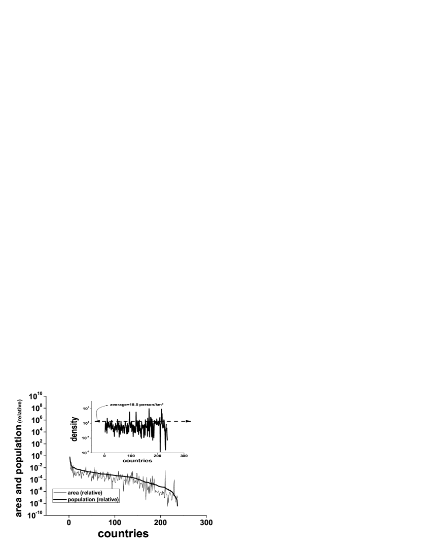
On Earth there are countries (states, where the provinces are disregarded), which have totally about few million cities, where more than 6 billion humans live and speak about languages, at present. The whole life goes on over an area of some million km2. Figure 1 is plotted utilizing the present empirical data [6] for the relative population of the countries (divided by the world population, thick line) in rank order; i.e., the most populous country (China) has the rank one, the next populous country (India) has the rank two, and the third populous country (USA) has the rank three, etc., where the corresponding relative area of the countries (divided by the area of the Earth) is designated by the plot in the thin line. The area plot depicts fluctuation; yet, it roughly follows the population line. The inset (Figure 1) is for the population density in capita per km2, which shows that the population density is almost constant (about capita per km2) over the countries.
Our essential aim in the present contribution is to show that the time evolution of the world with her cities, languages and countries, etc., might be governed by two opposite processes: random multiplicative noise for growth in size and fragmentation for spread in number and extinction. Secondly, we aim at obtaining a wide panorama for the world (cities, languages, countries and their distributions, lifetimes, etc.) in terms of a single simulation, where the related results are obtained at the same time. The model is developed in [3], where the cities and the languages are treated differently and as connected; languages split since cities split, etc. (For a quantitative method for the formation of the languages, please see references in [3].) Results for the size distribution functions, the probability distribution functions (PDF) and various other functions for both the cities and the languages are found to be in good agreement with the empirical data. Yet, the results for the language families (in [3]) are considerably far from reality.
In the present work, our focus is on the families; here the size distributions of the families for both the cities (countries) and the languages are given besides their distributions over the number of their members, etc. In [3], the number of the language families was not changing in time and the city families were not considered at all. Here, both the offspring cities and the languages may create new families; in other words, the current families may fragment as explained in Sec. 3.3. Secondly, we apply random punctuation for the cities and random change of the languages, which was not followed in [3]. We now also study bilinguals.[7] Thus, we present here a richer panorama of the world, where all of the results are obtained in the same simulation, at the same time for many parameters.
The following section is the model, and the next one is the applications and results. The last section is devoted for discussion and conclusion. Appendix is a brief description of the model, which is given extensively in [3].
2 Model:
This section is the definition (2.1.) and a brief review (2.2.-2.4.) of the model, where also introduced are the meaning of the relevant concepts and the parameters, with the symbols in capital letters for the cities and those in lower case for the languages. The subscript fam is used for the families.
The initial world has ancestors for the cities and ancestors for the languages , with . Each city has a random size and she speaks one of the initial languages, which is selected randomly. So, is the population of each ancestor city, and is the number of people speaking each ancestor language. (It is clear that the total number of the citizens and the speakers is the same and it is equal to the initial world population.)
2.1 Definition:
Populations of the cities grow in time , with a random rate , where is universal within a random multiplicative noise process,
As the initial cities grow in population the initial languages grow in size , where the cities (and consequently, the languages) fragment in the meantime. If a random number (between 0 and 1; defined differently at each time step ) for a city is larger than some close to , then the city becomes extinct (random elimination, punctuation); otherwise, if it is smaller than some small , the city splits after growing, with the splitting ratio (fragmentation, mutation factor) : If the current number of habitants of a city is , many members form another population and many survive within the same city. The number of the cities increases by one if one city splits; if any two of them split at , then increases by two, etc. When a city is generated she speaks with probability a new language, with probability a randomly selected current language, and with the remaining probability the old language (of the mother city).
2.2 Lifetimes for cities or languages:
Lifetime is the difference between the number of the time step at which a city or a language is generated and that one at which the given agent became extinct. The agent becomes extinct if its size becomes less then unity in terms of fragmentation or if it is randomly eliminated (with ). If all the cities which were speaking a given language are eliminated (by any means), then we consider the given language(s) as eliminated. And, if all the members of a family become extinct (by any means), then we consider the family as extinct. The age of a living agent (at the present) is considered as the time passed from the time of their formation up to now.
2.3 Family trees for the cities or the languages:
We construct the family trees for the cities and the languages as follows: We assume that the initial cities and the initial languages have different families; i.e., we have many city families and many language families at t=0. We label each city by these numbers, i.e. the city family number and the language family number, which may not be the same later (for example, due to long and mass immigration, as in reality). In this manner, we are able to compute the number of the members of each family, as well as their sizes at the present time, etc. (The given labels may be also utilized to trace the generation level of the offspring agents.) It is obvious that the unification (merging) of the cities or the languages are kept out of the present scope.
2.4 Bilinguals:
Some citizens of a given city (country) may select another language (other than the common or official language of the home city, home country, i.e., the mother tongue) to speak, where several reasons may be decisive. We consider here the size distribution of the second languages (bilinguals [7]), where we assume that an adult (speaking a language as a mother tongue) selects one of the current languages if this language is bigger than the mother language, . Then
where, and the prime denotes the second language. In Eq. (2) is a random number which is uniformly distributed between zero and one. So; for a given , which is proportional to the percentage (up to randomness) of the population of the language the speakers of which select as the second language, and is taken as universal. It is obvious that, has the unit per capita (person) and as the size difference increases, the language becomes more favorite and the related percentage increases.
3 Applications and results:
The parameters for the rates of growth (Sect. 2, with the symbols in capital letters for the cities and these in lateral ones for the languages) have units involving time: here, the number of the interaction tours may be chosen as arbitrary (without following historical time, since we do not have historical data to match with); and the parameters (with units) may be refined accordingly. Yet, our initial conditions (with the given initial parameters for ancestors) may be considered as corresponding to some years ago from now. So the unit for our time steps may be taken as (about) years, since we consider time steps for the evolution. After some period of the evolution in time we (reaching the present) stop the computation and calculate PDF for size, and for some other functions such as extinction frequency, lifetime, etc. (for the cities or the languages and their families, etc.).
Empirical criteria for our results are: i) The number of the living cities (towns, villages, etc.) and that of the living languages may be different; but, total size for the present time must be the same for both cases (and also for the families of the cities or the languages), where the mentioned size is the world population (Eqn. (2)). ii) World population increases exponentially with time.[4, 5, 6] iii) At present, the biggest language (Mandarin Chinese) is used by about billion people and world population (as, the prediction made by United Nations) is billion in , (and will be about billion in ) [4, 5, 6]; so the ratio of the size for the biggest language to (the total size, i.e.,) world population must be (about) . iv) Size distribution for the present time must be power law –1 for the cities (Pareto-Zipf law), and this may be considered as slightly asymmetric log-normal for the languages. We first consider the cities (Sect. 3.1), later we study the languages (Sect. 3.2), with the lifetimes, etc., in all; and the families are considered finally (Sect. 3.3).
3.1 Cities:
The initial world population () is about , since the average of uniform random numbers between zero and unity is 1/2. Thus, we assume power law zero for the initial distribution of the cities or the languages over size.
We tried many smooth (Gauss, exponential, etc.) initial distributions (not shown); and, all of them underwent similar time evolutions within 2,000 time steps, under the present processes of the random multiplication for growth, and random fragmentation for spread and origination and extinction, where we utilized also various combinations of the parameters and . We tried also delta distribution, which is equivalent to assuming a single ancestor, for the initial case; it also evolved into a power law about –1 (with different set of parameters, not shown) in time. Since we do not have real data for the initial time, we tried several parameters for (=1,000; 300; 50, etc.) and for (=1,000; 500) at . In all of them, it is observed that the city distribution at present (Pareto-Zipf law) is independent of the initial (probable) distributions, disregarding some extra ordinary ones. Please note that, similar results may be obtained (not shown) for , i.e., single ancestor.
Evolution: As increases, the cities start to be organized; and within about 200 time steps, we have a picture of the current world which is similar to the present world, where the distribution of the cities over population is considerably far from randomness. With time, the number of the cities () and the population of the world () increases exponentially with different exponents.[3] Please note that these simulations have about two million cities and the world population comes out as about 4.5 billion at (present time, the year 2000), for , , , , and . With another set of the parameters; for , and (keeping other parameters same as before) we have about 450 thousand () cities with billion total citizens (), etc.
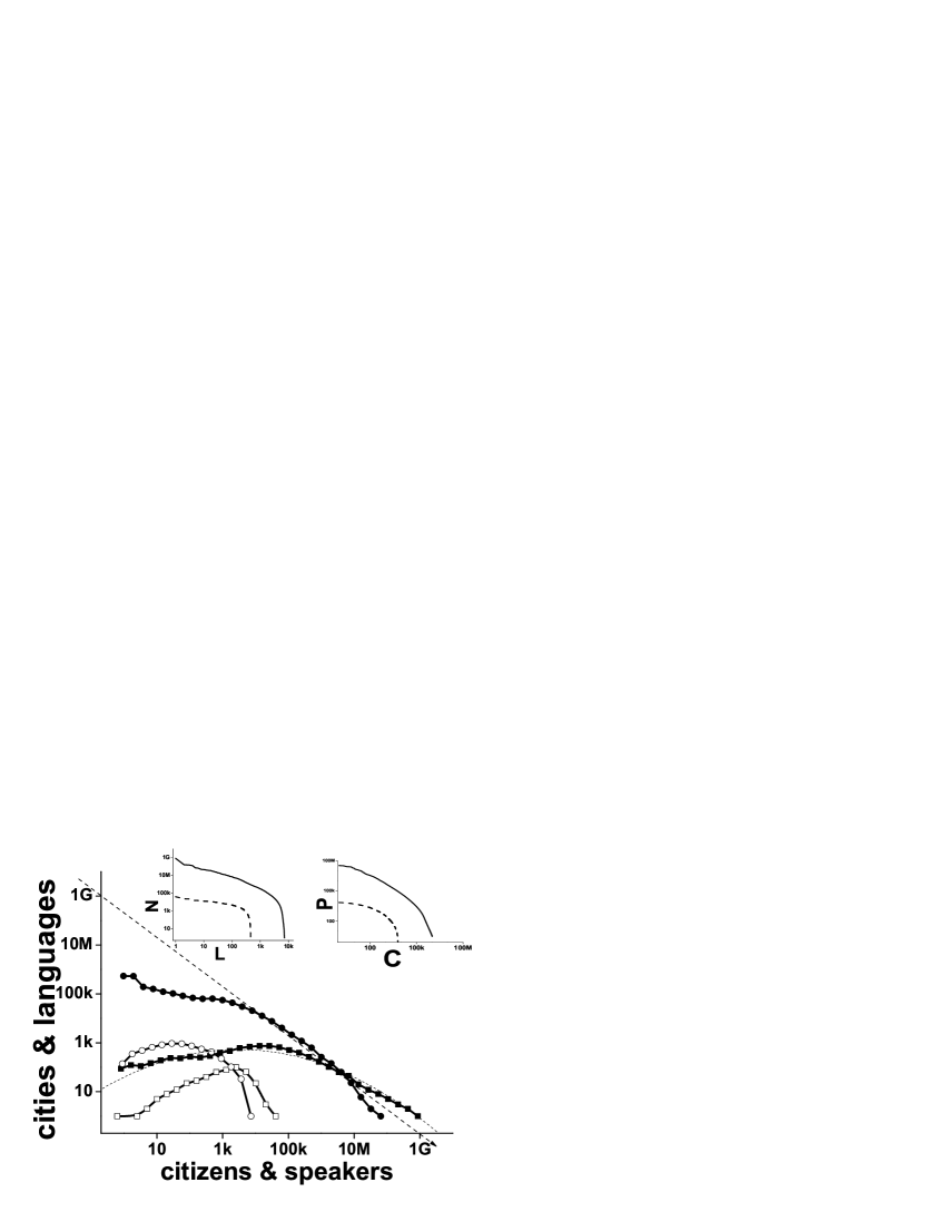
In Figure 2 the plots in circles (open ones for and solid ones for ) represent the time evolution of size distribution of the cities (PDF), all of which split and grow by the same parameters (Set 1), where . Thus, we have abrupt (punctuated) elimination of the cities here, which is not followed in [3]; yet the results are not much different, because the punctuation we applied here is light (low). This means that it is not strong enough to disturb the running processes, where the negative effect of the (light) punctuation (in decreasing the numbers) is diminished by the positive effect of the fragmentation (in increasing the numbers). Please note that, in Fig.2 the (dashed) arrow has the slope –1, which indicates the (empirical) Pareto-Zipf law for the cities.
Furthermore, we observe that, as the initial cities spread in number by fragmentation, the initial random distribution turns out to be log-normal for intermediate times (as the parabolic fit indicates, for for example) which becomes a power law –1 (at tail, i.e., for big sizes) for the present time. The inset (right) in Fig. 2 is the distribution of the world population () at (dashed line) and (solid line) over the cities (), which are in rank order along the horizontal axis. Please note that, in the figure and in the inset, axes are logarithmic. It may be observed in the plots in the inset (Fig. 2, right) that, the world population (along the vertical axis, ) increases slightly more rapidly than the number of the cities (along the horizontal axis, ). So, Fig. 2 may be considered as the summary for history of the evolution of the cities (or the languages, see Section 3.2.), where two opposite physical processes underline the evolution; the random multiplicative noise and the fragmentation.
Lifetimes: We obtain the time distribution of the cities (lifetime for extinct cities and ages of the livings ones, not shown here) as decreasing exponentials (disregarding the cases for small number of ancestors and high punctuation) as given in the related figures in [3]. Simple probability (density) functions for the lifetimes are also exponential (not shown), which means that the cities occupy the time distribution plots in exponential order; more cities for small , and fewer cities for big , for a given number of time steps in all.
3.2 Languages:
We guess that there were many simple languages (composed of some fewer and simple words and rules), which were spoken by numerous small human groups (families, tribes, etc.) at the very beginning. And, as people came together in towns, these primary languages might have united. Yet, we predict that the initial world is not (much) relevant for the present size configuration of the languages (as well as in the case for cities; see, Sect. 3.1). Moreover, we may obtain similar target configurations for different evolution parameters (not shown). Within the present approach, the ancestor cities and the ancestor languages are associated randomly; since, the languages with their words, grammatical rules, etc. might have been formed randomly ([3], and references therein); the societies grew and fragmented randomly (as mentioned in Sect. 2); new cities randomly formed new languages or changed their language and selected a new one randomly. We predict that, the index (roughly) decreases as increases for small (not shown). We predict also the distribution of the present languages over the present cities, where we have power law minus unity (not shown). It may be worthwhile to remark that, younger cities prefer younger languages; which means also that the new cities (or the new countries which are composed of the new cities) emerge mostly with new languages. Secondly, as increases the indices and increase, and the plot of versus extends upward and moves rightward, since the number of the current languages () and the number of cities, which speak a given language, increase (as a result of the fragmentation of the cities).
Furthermore, we compute the number (abundance) of the speakers for the present languages (, in Eq. (2)) (not shown), where we have few thousand () living languages. Within this distribution of the present languages over the speakers, we predict power law minus unity (not shown). It may be worthwhile to remark that older languages have more speakers; and in reality (Mandarin) Chinese, Indian, etc., are big and old languages. For example, we have about one billion people speaking the language number 1, which is one of the oldest languages of the world; and less people speaking the language number 2, etc.
In Figure 2, we display the PDF for the size distributions of the languages at (historical, open squares) and (present, solid squares), where the number of the ancestor languages () is 300. We plotted several similar curves for i.e., for the case where only one ancestor language is spoken in each ancestor city and obtained similar results (not shown). Splitting rate and splitting ratio for languages are not defined here, since languages split as a result of splitting of the cities; and the splitting ratio of the splitting language comes out as the ratio of the population of the new city (which creates a new language) to the total population of the cities which speak the fragmented language. Please note that, in the plots (Fig.2) for the languages at the present time (solid squares for ) we have slightly asymmetric Gauss for big sizes as the parabolic fit (dashed line) indicates; and we have an enhancement for the small languages in agreement with reality [8]. Fig. 2 may be considered as the summary for history of the evolution of the cities and the languages.
We think that, the (random) elimination of the languages (with all of its speakers) is not realistic (excluding the small languages with small number of speakers), and it is not recorded in the history for the recent times. On the other hand, changing (replacing) a language by another one may be realistic. And, in case of random (light) elimination (i.e., changing the language with a current one), the fragmentation rate may accordingly be increased to obtain the empirical data for the number of the languages at the present. In other words, the number of the languages increases by and decreases by , which may be considered as punctuation for the languages with . In Fig. 2 (and in other related ones) we utilized and .
Lifetimes for the languages and the related probability densities are decreasing exponentially (as for the cities); which means that many languages (cities) become extinct soon after they emerge and the remaining ones live long (not shown) as in reality. Please see Fig. 2 in [8] for the related empirical data. The (negative) exponent of the present decay is about per time step for time steps.
3.3 Families of the cities (countries) or the languages and the bilinguals:
We obviously do not know how the city (language) families [9] are distributed over the cities (languages) initially; since, we do not have any historical record about the issue. Yet, we predicted that the initial conditions for the cities (languages) are almost irrelevant for the present results. And we considered several initial conditions for the city families and the language families, which are discussed in [8] to some extent in empirical terms.
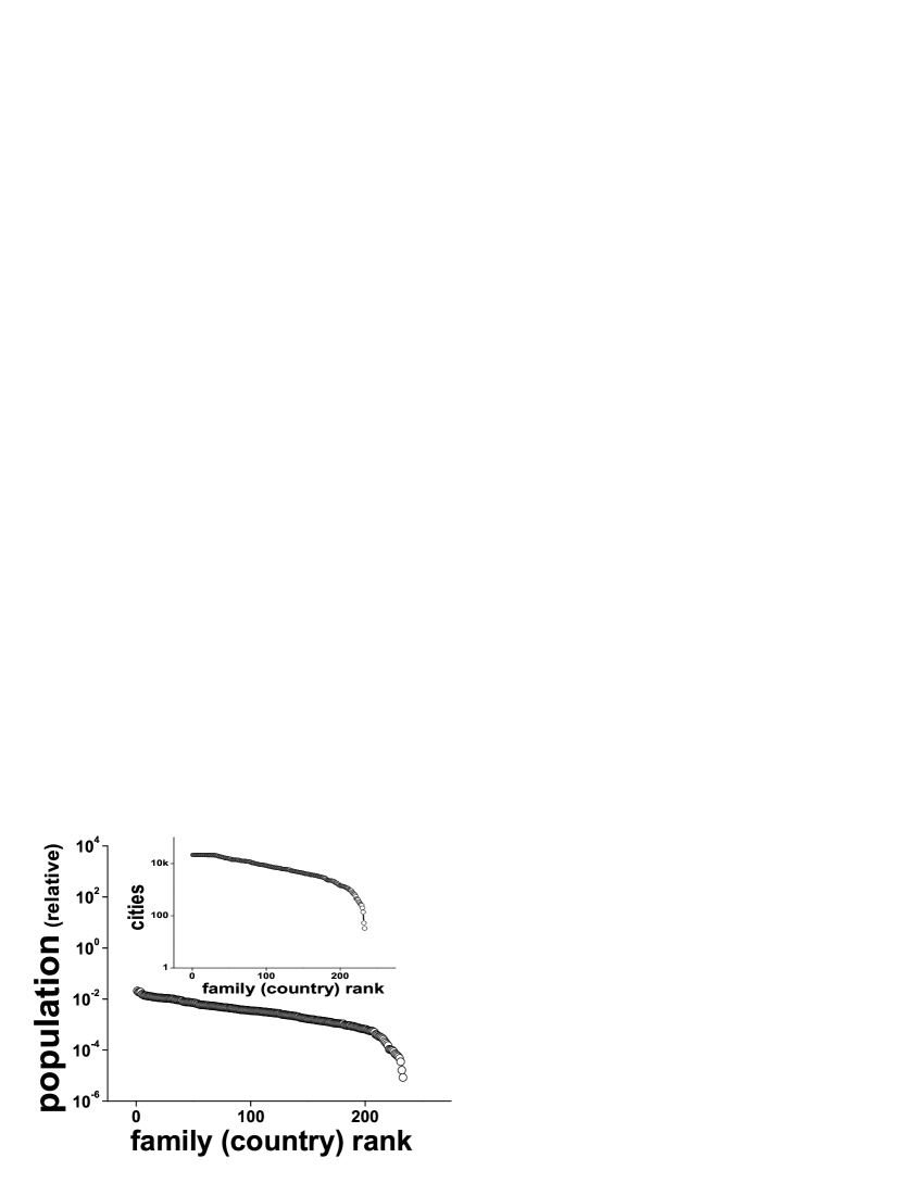
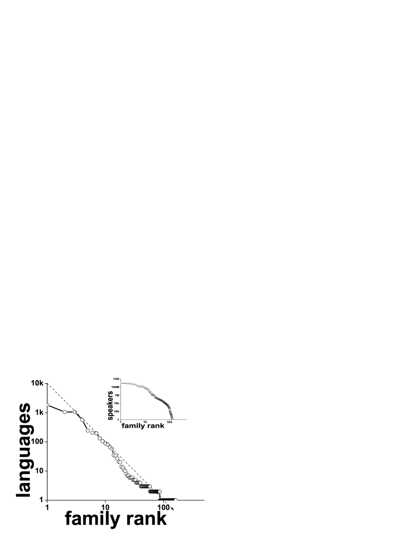
We think that, the number of the city families and the language families were roughly the same, (yet, the number of the cities and the languages might be different) initially; and we take , (for and . Figure 3 and Figure 4 are for the city families and the language families, with , and , all respectively; where, other parameters are as before. Figs. 3 and 4 may be considered as in good agreement with the empirical plots in Fig. 1 (and in refs. [4, 5, 6]). Please note that, the families evolve in time here (with the parameters given for the related fragmentation in this paragraph), which is not considered in [3]. For the bilinguals we assume that a small fraction of the citizens selects a second language out of the bigger ones and the introduced probability increases with the difference in sizes. Figure 5 is the PDF for the distribution of the bilinguals over the relative population (to the total), where Eq. (3) is utilized with the present languages (Figs. 2 and 4) for . We observe in Fig. 5 that few big languages are favored as the second language by the majority (about 90 %) of the speakers, with the given . We think that selecting big languages as second languages may help increase the sizes of the big languages.
4 Discussion and conclusion:
Starting with random initial conditions and utilizing many parameters in two random processes (the multiplicative noise for growth and the fragmentation for generation and extinction of the cities or the languages) for the evolution, we obtained several regularities (for size and time distributions, etc.) within the results; all of which may be considered as in good agreement with the empirical data.
We predict that the results are (almost) independent of the initial conditions, disregarding some extra ordinary ones. Furthermore, punctuation (besides fragmentation) eliminates the ancestors, with time. For (), we need longer time to mimic target configuration (if other parameters are kept the same as before), where new generated cities or languages may be inserted, in terms of fragmentation, provided , and .
Many cities or languages become extinct in their youth, and less become extinct as they become old. In other words, languages or cities become extinct either with short lifetime (soon after their generation), or they hardly become extinct later and live long (which may be considered as a kind of natural selection). We consider the mentioned result (which is observed in reality [8])as an important prediction of the present model and we had obtained similar results for the evolution biological species [10], which may be coming out because of the present random multiplicative noise and fragmentation processes.
It might be argued (objected, by the reader) that, there are many parameters in the model. Each of them is needed for some measure of the related evolution in reality. Secondly, as we predict that the initial conditions are (almost) irrelevant for the present results and many parameters (for ) may be ignored. Thirdly, the most important parameter in the model is (the rate for population growth), and is related to implicitly, since we need more cities to be established (per time) as the world population increases. The punctuation parameter may also be considered as a parameter dependent (implicitly) on ; since the probability for the emergence and spread of wars, illnesses, etc. increases, as world population increases. The rates for the languages (, , etc.) may also depend (implicitly) on ; since more new languages (per time) are needed with the increasing world population, etc. The rates for the families certainly depend on the number of their current members, the rate of which may (ultimately) be controlled by . Speaking geometrically, the area under each plot for the size distribution of the cities, languages, language families, city families (countries) must always equal to the world population at any time ; and this constraint constructs the bridge for the given implicit dependence of the rate parameters (for the considered functions) on .
As a final remark we claim that the original model may be useful to predict also the historical size distribution of the cities: We predict that the initial distribution of the cities over the population becomes parabolic for some intermediate time () in log-log scale and it turns to be power law –1 as time goes on (i.e., for the present time; ). The mentioned distribution may be checked within the archaeological data (as a subject of a potential field of science; namely, physical history) for the ancient cities (towns); where, the time evolution of the mentioned distribution into power law –1 may also be considered.
5 APPENDIX
In the present model, we have (with the symbols in capital letters for the cities and those in lower case for the languages; and the sub index fam is used for the families) ancestors for the cities and ancestors for the languages , with . Each city has a random size () and she speaks one of the initial languages, which is selected randomly. So, () is the population of each ancestor city, and is the number of people speaking each ancestor language. It is clear that the total number of the citizens and the speakers is same (for any ) and it is equal to the current world population;
The cities have fixed growth rates (), which are distributed randomly over the ancestors and they (and, these for the offspring; where the offspring carry the same growth rate as their ancestors) are not changed later; yet, the maximum value () for the growth rates is constant for all of the cities (so is for world). Furthermore, we have initial city families and initial language families, with . Please note that, all of the introduced parameters are about physical quantities, which represent several situations in reality.
The time evolution of the cities (or the languages and their families) is considered in terms of two random processes, the multiplicative random noise [1] and the random fragmentation [2], which are coupled; here, the cities or the languages (and their families) are taken as a whole and the individuals are ignored. The cities grow in number by splitting (with constant ratio ) where, the fragmentation rate is ; and, the languages, the city families and the language families follow them accordingly, with various fragmentation rates: If a new city forms a new language () then it means that, the language of the home city is fragmented; here, the splitting ratio () is the ratio of the population of this new city to the total population of the cities which speak the old language. It is obvious that is small (); yet, many new languages may emerge at each time step, since many new cities emerge in the mean time, and becomes important. On the other hand, a new (and an old) city may change her language and select one of the current languages as the new one (with , for all), where colonization may take place or teachers may teach the new language [3], etc. In this case, size of the old (new) language decreases (increases) by the population of the new city. The language which is spoken by many cities has a higher chance for being selected by a new city; and so, big languages are favored in case of selecting a new language.
We consider the countries (city families) as follows: When a city is newly generated she establishes a new country (state, as we know many historical examples where each city was a state (city-state) and many new countries started with a new city) with probability ; with probability she is colonized (i.e., changes country); and, with the remaining probability she continues to survive within the home country. It is obvious that when a city (or a group of cities, due to the present randomness) starts a new country, it means that the old country is fragmented. Secondly, not only the newly generated cities but also the old ones may be colonized. The countries with all of her cities may also be colonized (conquered) as we know from many examples in history. Similar treatment may cover the language families with the parameters , and (the probability for starting a new language family, for changing the language (and so the language family, while surviving within the home country, i.e., being culturally colonized) and for continuing to speak a language which belongs to the home language family; respectively).
Please note that, the fragmentation causes new agents to emerge (birth), and at the same time it drives them to extinction in terms of splitting, and any agent with a member less than unity is considered as extinct. The number of the cities increases, decreases, or fluctuates about for relatively big numbers for (high fragmentation) and (low elimination), for small numbers for (low fragmentation) and (high elimination), and for (equal fragmentation and elimination), respectively; out of which we regard only the first case, where we have (for ) an increase in the number of cities, and we disregard the others. We try several numbers of the ancestors , with sizes , where we assign new random growth rates for the new cities, which are not changed later, as well as the growth rates for ancestors are kept as same through the time evolution.
It is obvious that gives the gradual evolution for the cities, where we have regular fragmentation with (and with some ) at each time step . This case is kept out of the present scope, because we consider it as (historically) unrealistic.
It may be worthwhile to stress that elimination (punctuation, ) plays a role which is opposite to that of fragmentation () and growth () in evolution; here, and develop the evolution forward, and recedes. So the present competition turns out to be the one between and , and , where two criteria are crucial: For a given number of time steps, , and , etc., there is a critical value for ; where, for cities survive, and for smaller values of (i.e., if ) cities may become extinct totally. (For similar cases in the competition between species in biology, one may see [10].) Secondly, sum of H and is a decisive parameter for the evolution: If for a given (with ), , then the number of cities does not increase and does not decrease, but oscillates about , since (almost) the same amount of cities emerges (by ) and becomes extinct (by ) at each time step, and we have intermediate elimination. On the other hand, if , then the cities decrease in number with time and we have high (strong, heavy) elimination. Only for (with ) we have low (weak, light) elimination of cities, where the number increases (yet, slowly with respect to the case for ). In summary, only light punctuation of the cities may be historically real, and it does not affect the evolution and size distribution of the cities, as we observed in many runs (not shown), where we increase the fragmentation () and population growth rate () to compensate the negative effect of punctuation on the number of cities and world population, respectively. Yet, the ancestor cities i.e., those at age of at any time , decay more quickly in time as (punctuation increases) decreases (since the generated cities may be substituted by new generated ones after elimination; but the ancestor ones can not be re-built.) It is obvious that punctuation of a city (together with all of the citizens) is realistic as many (regrettable) examples occurred during many wars.
References
- [1] H.A. Simon, Models of Man, Wiley, New York 1957
- [2] V. Novotny and P. Drozdz, Proc. Roy. Soc. London B 267, 947, (2000).
- [3] Ç. Tuncay, Physics of randomness and regularities for cities, languages, and their lifetimes and family trees, to be published in Int. J. Mod. Phys. C 18, (2007), e-print 0705.1838 on arXiv.org
- [4] URL: http://linkage.rockefeller.edu/wli/zipf/; http://linkage.rockefeller.edu/wli/zipf/index_ru.html; http://www.nslij-genetics.org/wli/zipf/index.html; http://www.un.org/esa/population/publications/WPP2004/2004Highlights finalrevised.pdf
- [5] B.F. Grimes, Ethnologue: Languages of the World (14th edn. 2000). Dallas, TX: Summer Institute of Linguistics. S. Wichmann, J. Linguistics 41, 117 (2005). D. Zanette, Adv. Complex Syst. 4: 281 (2001).
- [6] URL: http://www.citypopulation.de/cities.html (For other useful sites: http://www.prb.org/; http://www.refdesk.com/factpop.html; http://www.census.gov/ipc/www/popclockworld.html
- [7] J. Mira, J., A. Paredes, Europhys. Lett. 69 (2005) 1031. 27. K. Kosmidis, J.M. Halley, P. Argyrakis, Physica A, 353 (2005) 595. K. Kosmidis, A. Kalampokis, P. Argyrakis, Physica A 366, 495 and 370, 808 (2006). X. Castelló, V.M. Eguíluz, M. San Miguel, New J.Phys. 8, 308 (2006).
- [8] W.J. Sutherland, Nature 423 (2003) 276.
- [9] P.M.C. de Oliveira et al. arXiv:0709.0868, submitted to J. Linguistics.
- [10] Ç. Tuncay, A physical model for competition between biological speciation and extinction, arXiv:q-bio.PE/0702040, submitted to J. Theo. Bio.