The critical behaviour of $3D$ Ising spin glass models: universality and scaling corrections

Abstract

We perform high-statistics Monte Carlo simulations of three three-dimensional Ising spin glass models: the $\pm J$ Ising model for two values of the disorder parameter $p$, $p=1/2$ and $p=0.7$, and the bond-diluted $\pm J$ model for bond-occupation probability $p_{b}=0.45$. A finite-size scaling analysis of the quartic cumulants at the critical point shows conclusively that these models belong to the same universality class and allows us to estimate the scaling-correction exponent $\omega$ related to the leading irrelevant operator, $\omega=1.0(1)$. We also determine the critical exponents $\nu$ and $\eta$. Taking into account the scaling corrections, we obtain $\nu=2.53(8)$ and $\eta=-0.384(9)$.

The most peculiar aspect of critical phenomena is the universality of the asymptotic behaviour in a neighborhood of the critical point. In experiments and Monte Carlo (MC) simulations the possibility of approaching the critical point (and/or the infinite-volume limit) is generally limited. Therefore, an accurate determination of the universal critical behaviour requires a good control of the scaling corrections. This is particularly important for systems with disorder and frustration, such as spin glasses, where severe technical difficulties make it necessary to work with systems of relatively small size. Even though the critical behaviour of Ising spin glass models has been much investigated numerically in the last two decades, see, e.g., [1, 2, 3, 4, 5, 6, 7, 8, 9, 10, 11, 12], it is not yet clear how reliable the numerical results are. For instance, the estimates of the critical exponents have significantly changed during the years, as shown by the results reported in [1]. Moreover, the most recent MC studies, see, e.g., [1, 2], find significant discrepancies among the estimates of the correlation-length exponent $\nu$ obtained from the finite-size scaling (FSS) at $T_{c}$ of different observables, such as the temperature derivatives of $\xi/L$, of the Binder cumulant, and of the susceptibility. For instance, for the bimodal Ising model [1] quotes $\nu=2.39(5)$, $\nu=2.79(11)$, and $\nu=1.527(8)$, from the analysis of these three quantities. These differences indicate the presence of sizeable scaling corrections. However, the data are not precise enough to allow for scaling corrections in the analyses. In order to reduce their effects, [2] has proposed an alternative purely phenomenological scaling form inspired by the high-temperature behavior, which affects only the analytic scaling corrections and apparently reduces the differences among the estimates of $\nu$. Some attempts to determine the nonanalytic scaling corrections have been reported in [10, 9, 8, 4], but results are quite imprecise.

Summarizing, little is known about the scaling corrections in Ising spin glass models, even though it is now clear that their understanding is crucial for an accurate determination of the critical behavior. Here we report a MC study, which represents a substantial progress in this direction. Indeed, by a FSS analysis of renormalisation-group (RG) invariant quantities we are able to obtain a robust estimate of the leading scaling-correction exponent $\omega$. This allows us to analyze the MC data for the critical exponents taking the scaling corrections into account. Estimates obtained from different observables are now in agreement.

We consider the $\pm J$ Ising model on a cubic lattice of linear size $L$ with periodic boundary conditions. The corresponding Hamiltonian is

$$H=-\sum_{\langle xy\rangle}J_{xy}\sigma_{x}\sigma_{y},$$ (1)

where $\sigma_{x}=\pm 1$, the sum is over pairs of nearest-neighbor lattice sites, and the exchange interactions $J_{xy}$ are uncorrelated quenched random variables with probability distribution $P(J_{xy})=p\delta(J_{xy}-1)+(1-p)\delta(J_{xy}+1)$. The usual bimodal Ising spin glass model [13], for which $[J_{xy}]=0$ (brackets indicate the average over the disorder distribution), corresponds to $p=1/2$. For $p\neq 1/2$, $[J_{xy}]=2p-1\neq 0$ and ferromagnetic (or antiferromagnetic) configurations are energetically favored. A reasonable hypothesis is that, along the transition line separating the paramagnetic and the spin glass phase, the critical behaviour is independent of $p$, i.e., a nonzero value of $[J_{xy}]$ is irrelevant, as found in mean-field models [14]. The paramagnetic-glass transition line extends for $p^{*}>p>1-p^{*}$, where [15] $p^{*}=0.76820(4)$. For $1>p>p^{*}$ the low-temperature phase is ferromagnetic, and the transition belongs to the randomly-dilute Ising universality class [16]. We also consider a bond-diluted $\pm J$ Ising model with bond-occupation probability $p_{b}=0.45$, and equal probability for the values $\pm J$.

We focus on the critical behaviour of the overlap parameter $q_{x}\equiv\sigma_{x}^{(1)}\sigma_{x}^{(2)}$, where $\sigma_{x}^{(i)}$ are independent replicas with the same disorder $J_{xy}$. If $G(x)\equiv[\langle q_{0}q_{x}\rangle]$, we define the susceptibility $\chi\equiv\sum_{x}G(x)$ and the second-moment correlation length $\xi$

$$\xi^{2}\equiv{1\over 4\sin^{2}(q_{\rm min}/2)}{\widetilde{G}(0)-\widetilde{G}(q)\over\widetilde{G}(q)},$$ (2)

where $q=(q_{\rm min},0,0)$, $q_{\rm min}\equiv 2\pi/L$, and $\widetilde{G}(q)$ is the Fourier transform of $G(x)$. We also define

$$R_{\xi}\equiv\xi/L,\quad U_{4}\equiv{[\mu_{4}]\over[\mu_{2}]^{2}},\quad U_{22}\equiv{[\mu_{2}^{2}]-[\mu_{2}]^{2}\over[\mu_{2}]^{2}},$$ (3)

where $\mu_{k}\equiv\langle\;(\sum_{x}q_{x}\;)^{k}\rangle$. The quantities (3) are RG invariant. We call them phenomenological couplings and denote them by $R$ in the following.

Let us first summarize some basic results concerning FSS, which allow us to understand the role of the analytic and nonanalytic scaling corrections. We consider two Ising spin glass systems coupled by an interaction $h\sum_{x}q_{x}=h\sum_{x}\sigma^{(1)}_{x}\sigma^{(2)}_{x}$, in a finite volume of linear size $L$. The singular part of the corresponding disorder-averaged free energy density ${\cal F}$, which encodes the critical behavior, behaves as

$${\cal F}_{\rm sing}(\beta,h,L)=L^{-d}F(u_{h}L^{y_{h}},u_{t}L^{y_{t}},\{v_{i}L^{y_{i}}\})$$ (4)

$$=L^{-d}f(u_{h}L^{y_{h}},u_{t}L^{y_{t}})+v_{\omega}L^{-d-\omega}f_{\omega}(u_{h}L^{y_{h}},u_{t}L^{y_{t}})+\ldots,$$

where $u_{h}$ and $u_{t}$ are the scaling fields associated respectively with $h$ and $t\sim T-T_{c}$ (their RG dimensions are $y_{h}=(d+2-\eta)/2$ and $y_{t}=1/\nu$), and $v_{i}$ are irrelevant scaling fields with $y_{i}<0$. The leading nonanalytic correction-to-scaling exponent $\omega$ is related to the RG dimension $y_{\omega}$ of the leading irrelevant scaling field $v_{\omega}\equiv v_{1}$, $\omega=-y_{\omega}$. The scaling fields are analytic functions of the system parameters—in particular, of $h$ and $t$—and are expected not to depend on $L$. Note also that the size $L$ is expected to be an exact scaling field for periodic boundary conditions. For a general discussion of these issues, see [17, 18] and references therein. In general, $u_{t}$ and $u_{h}$ can be expanded as

$$u_{h}=h\bar{u}_{h}(t)+O(h^{3}),\quad\bar{u}_{h}(t)=a_{h}+a_{1}t+O(t^{2}),$$ (5)

$$u_{t}=c_{t}t+c_{02}t^{2}+c_{20}h^{2}+c_{21}h^{2}t+O(t^{3},h^{4},h^{4}t),$$

where we used the fact that the free energy is symmetric under $h\to-h$. In the expansion of $u_{h,t}$ around the critical point $h,t=0$, the terms beyond the leading ones give rise to analytic scaling corrections. There are also analytic corrections due to the regular part of the free energy; since they scale as $L^{\eta-2}\sim L^{-2.4}$, they are negligible in the present case. The scaling behaviour of zero-momentum thermodynamic quantities can be obtained by performing appropriate derivatives of ${\cal F}_{\rm sing}$ with respect to $h$. For instance, the overlap susceptibility $\chi=\partial^{2}{\cal F}/\partial h^{2}|_{h=0}$ behaves as

$$\chi=L^{2-\eta}\bar{u}_{h}(t)^{2}g(u_{t}L^{y_{t}})+L^{2-\eta-\omega}g_{\omega}(u_{t}L^{y_{t}})+\ldots$$ (6)

The FSS of the phenomenological couplings is given by

$$R(\beta,L) = r(u_{t}L^{y_{t}})+r_{\omega}(u_{t}L^{y_{t}})L^{-\omega}+\ldots$$ (7)

$$= R^{*}+r^{\prime}(0)c_{t}\,tL^{y_{t}}+\ldots+c_{\omega}\,L^{-\omega}+\ldots,$$

where $R^{*}\equiv r_{0}(0)$ and $c_{\omega}=r_{\omega}(0)$. In the case of $U_{4}$, this behaviour can be proved by taking the appropriate derivatives of ${\cal F}$ with respect to $h$. A similar discussion applies to $U_{22}$ and $\xi/L$, see Sec. 3.1 of [18] for details. The exponent $\nu$ can be computed from the FSS of the derivative $R^{\prime}\equiv dR/d\beta$ at $\beta_{c}$, or from that of the ratio $\chi^{\prime}/\chi$, where $\chi^{\prime}\equiv d\chi/d\beta$. At $T=T_{c}$, setting $t=u_{t}=0$ in the above-reported equations, we obtain:

$$R=R^{*}+c_{1}L^{-\omega}+\ldots,$$ (8)

$$\chi=cL^{2-\eta}(1+c_{1}L^{-\omega}+\ldots),$$ (9)

$$R^{\prime}=cL^{1/\nu}(1+c_{1}L^{-\omega}+\ldots),$$ (10)

$$\chi^{\prime}=cL^{2-\eta+1/\nu}(1+c_{1}L^{-\omega}+\ldots+a_{1}L^{-1/\nu}+\ldots).$$ (11)

Note that, unlike the temperature derivative $R^{\prime}$ of an RG invariant quantity, $\chi^{\prime}$ also presents an $L^{-1/\nu}$ scaling correction, due to the analytic dependence on $t$ of the scaling field $u_{h}$ (for this reason we call it analytic correction). Since, as we shall see, $1/\nu\approx 0.4$ and $\omega\approx 1.0$, the scaling corrections in $\chi^{\prime}$ decay slowlier than those occurring in $R^{\prime}$. This makes $\chi^{\prime}/\chi$ unsuitable for a precise determination of $\nu$ and explains the significant discrepancies observed in [1].

Instead of computing the various quantities at fixed Hamiltonian parameters, we consider the FSS keeping a phenomenological coupling $R$ fixed at a given value $R_{f}$ [19, 18]. This means that, for each $L$, we determine $\beta_{f}(L)$, such that $R(\beta=\beta_{f}(L),L)=R_{f}$, and then consider any quantity at $\beta=\beta_{f}(L)$. The value $R_{f}$ can be specified at will, as long as $R_{f}$ is taken between the high- and low-temperature fixed-point values of $R$. For generic values of $R_{f}$, $\beta_{f}$ converges to $\beta_{c}$ as $\beta_{f}-\beta_{c}=O(L^{-1/\nu})$, while at $R_{f}=R^{*}$, cf. (8), $\beta_{f}-\beta_{c}=O(L^{-1/\nu-\omega})$. One can easily show that the FSS behaviour at fixed $R_{f}=R^{*}$ is given by the same general formulas derived at $T_{c}$. In the case of another phenomenological coupling $R_{\alpha}$ we have

$$\bar{R}_{\alpha}(L)\equiv R_{\alpha}[\beta_{f}(L),L]\approx\bar{R}_{\alpha}^{*}+c_{\alpha}L^{-\omega}+\ldots,$$ (12)

where $\bar{R}_{\alpha}^{*}$ is universal but depends on $R_{f}$. If $R_{f}$ differs from $R^{*}$, $\chi$ and $R^{\prime}$ (but not the phenomenological couplings $R$) also present $L^{-k/\nu}$ corrections with amplitudes proportional to $(R_{f}-R^{*})^{k}$.

Table 1: Parameters for the simulations of the $\pm J$ model at $p=0.5$ for $L\geq 12$. We use the random-exchange method with $N_{\beta}$ temperatures between $\beta_{\rm min}$ and $\beta_{\rm max}=0.895$. An elementary iteration is composed by $n_{\rm met}$ Metropolis full sweeps of all $N_{\beta}$ systems followed by a temperature-exchange attempt of all pairs corresponding to nearby temperatures. The length of the each run is $48n_{\rm iter}$ iterations; the first $20n_{\rm iter}$ are discarded for equilibration. The total number of Metropolis sweeps per sample and $\beta$ is $n_{\rm tot}=48n_{\rm iter}n_{\rm met}$. The CPU time refers to a single core of a dual-core 2.4 GHz AMD Opteron processor.

$L$	samples/64	$n_{\rm met}$	$n_{\rm iter}$	$n_{\rm tot}/10^{3}$	$N_{\beta}$	$\beta_{\rm min}$	CPU time in days
12	106812	10	400	192	10	0.54	308
13	38282	10	600	288	10	0.54	210
14	31600	50	200	480	10	0.62	361
16	24331	10	1000	480	20	0.52	831
20	1542	20	2000	1920	32	0.5125	658
24	717	25	2500	3000	32	0.5125	826
28	285	60	2500	7200	20	0.6575	782

In the MC simulations we employ the Metropolis algorithm, the random-exchange method [20], and multispin coding. We simulate the $\pm J$ Ising model at $p=0.5$ for $L$=3-14,16,20,24,28, at $p=0.7$ for $L$=3-12,14,16,20, and the bond-diluted model at $p_{b}=0.45$ for $L$=4-12,14,16. We average over a large number $N_{s}$ of disorder samples: $N_{s}\approx 6.4\cdot 10^{6}$ up to $L=12$, $N_{s}/10^{3}\approx 2400,2000,1500,100,46,18$, respectively for $L=13,14,16,20,24,28$ in the case of the $\pm J$ Ising model at $p=0.5$. See Table 1 for details. Similar statistics are collected at $p=0.7$, while for the bond-diluted model statistics are smaller (typically, by a factor of two for the small lattices and by a factor of 6 for the largest ones). For each $L$ and model we perform runs up to values of $\beta$ such that $R_{\xi}(\beta,L)$ is approximately 0.63, which is close to the estimates of $R_{\xi}^{*}$ of [1]: 0.627(4) and 0.635(9) for an Ising model with bimodal and Gaussian distributed couplings, respectively. We carefully check thermalization by using the recipe outlined in [1]. Estimates of the different observables for generic values of $\beta$ close to $\beta_{c}$ are computed by using their second-order Taylor expansion around $\beta_{\rm max}=0.895$. We check the correctness of these estimates by comparing them with those obtained by using the Taylor expansion around the value of $\beta$ used in the random-exchange simulation that is closest to $\beta_{\rm max}$. In total, the MC simulations took approximately 30 years of CPU-time on a single core of a 2.4 GHz AMD Opteron processor.

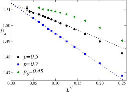
Figure 1: Phenomenological coupling $\bar{U}_{4}(L)$ vs $L^{-1}$. The lines are drawn to guide the eye.

We first perform a FSS analysis at fixed $R_{\xi}=0.63$. For sufficiently large $L$, the FSS behaviour of $\bar{U}_{4}$ and $\bar{U}_{22}$ is given by (12). The MC estimates of $\bar{U}_{4}(L)$ are shown in Fig. 1 versus $1/L$. The results for the $\pm J$ Ising model at $p=0.5$ and $p=0.7$ fall quite nicely on two straight lines approaching the same point as $L\to\infty$, indicating that $\omega\approx 1.0$. In the case of the diluted model the approach to the large-$L$ limit is faster: fits give $\bar{U}_{4}(L)=\bar{U}^{*}_{4}+eL^{-\epsilon}$ with $\epsilon\approx 2$. This indicates that $c_{4}\approx 0$ [see (12)]. According to the RG, this implies that the leading nonanalytic scaling correction is suppressed in any quantity. Thus, the approach to the critical limit should be faster, as already noted in [3]. We fit the data to $\bar{U}^{*}+cL^{-\epsilon}$, taking $\epsilon$ as a free parameter. Using data for $L\geq L_{\rm min}=8$, we obtain $\bar{U}_{4}^{*}=1.514(1)$, $\bar{U}_{4}^{*}=1.514(2)$, and $\bar{U}_{4}^{*}=1.513(1)$ for the $\pm J$ model at $p=0.5$ and $p=0.7$, and the bond-diluted model, respectively. The fits of $\bar{U}_{22}$ to $\bar{U}^{*}_{22}+cL^{-\epsilon}$ ($L_{\rm min}=6$) give $\bar{U}_{22}^{*}=0.1477(3)$, $\bar{U}_{22}^{*}=0.1481(8)$, and $\bar{U}_{22}^{*}=0.1479(6)$, respectively for the $\pm J$ Ising model at $p=0.5$ and $p=0.7$, and the bond-diluted model. These results represent a very accurate check of universality.

The analyses of $\bar{U}_{4}$ and $\bar{U}_{22}$ give also estimates of $\omega$. The most precise ones are obtained from the analysis of $\bar{U}_{4}$. In Fig. 2 we show the results for $\omega$ as obtained from fits of $\bar{U}_{4}$ to $\bar{U}^{*}_{4}+c_{p}L^{-\epsilon}$ and of fits of the difference $\bar{U}_{4}(p=0.5;L)-\bar{U}_{4}(p=0.7;L)$ to $bL^{-\epsilon}$. To verify the stability of the results, we have repeated the fits several times, each time including only the data satisfying $L\geq L_{\rm min}$. We estimate $\omega=1.0(1)$. As a check, we verify that the ratio $c_{22}/c_{4}$ is universal [$c_{\#}$ is the scaling-correction amplitude appearing in (12)], as predicted by standard RG arguments. Fits of $\bar{U}(L)-\bar{U}^{*}$ to $cL^{-\epsilon}$, fixing $\bar{U}_{4}^{*}=1.514$, $\bar{U}_{22}^{*}=0.148$, $\epsilon=1.0$ ( $L_{\rm min}=12$) give $c_{22}/c_{4}=0.19$ and $c_{22}/c_{4}=0.20$, respectively for $p=0.5$ and $p=0.7$, which are in good agreement.

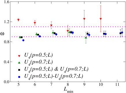
Figure 2: Estimates of the leading scaling-correction exponent $\omega$. For each $L_{\rm min}$, they are obtained by fitting only the data satisfying $L\geq L_{\rm min}$. The dotted lines correspond to the final estimate $\omega=1.0(1)$.

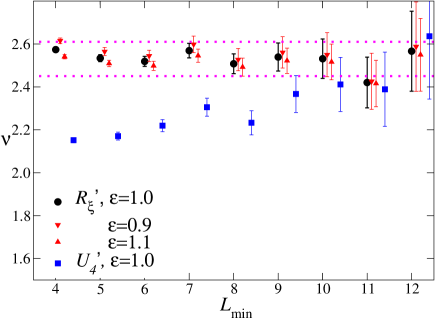
Figure 3: Estimates of the exponent $\nu$ from the FSS analysis of $R_{\xi}^{\prime}$ and $U_{4}^{\prime}$, for the $\pm J$ Ising model at $p=0.5$, obtained by fitting the data to (13). The dotted lines correspond to the final estimate $\nu=2.53(8)$.

Equation (12) holds for any chosen value of $R_{f}$. On the other hand, $\chi$ and $R^{\prime}$ do not present $O(L^{-1/\nu})$ corrections only if $R_{f}=R^{*}$. Thus, before computing the critical exponents, we refined the estimate of $R_{\xi}^{*}$ by performing a standard FSS analysis of $R_{\xi}$ which takes into account the scaling corrections. Fixing $\omega=1.0(1)$, we obtained $R_{\xi}^{*}=0.654(7)$, which is slightly larger than the estimates reported in [1, 3]. For the $\pm J$ model at $p=0.5$ we also obtained $\beta_{c}=0.908(4)$. Then, in order to determine the critical exponent $\nu$, we computed $R_{\xi}^{\prime}$ and $U_{4}^{\prime}$ at fixed $R_{\xi,f}=0.654$. In Fig. 3 we show results for the $\pm J$ Ising model at $p=0.5$, obtained by fitting $R_{\xi}^{\prime}$ to

$${\rm ln}R^{\prime}=a+{1\over\nu}{\rm ln}L+bL^{-\epsilon},$$ (13)

with $\epsilon=\omega=1.0(1)$, as a function of $L_{\rm min}$. They are quite stable and lead to the estimate

$$\nu=2.53(6)[2],$$ (14)

where the error in brackets takes into account the uncertainty on $\omega$. Since $R_{\xi,f}=0.654$ is only approximately equal to $R_{\xi}^{*}$, we may have residual $L^{-1/\nu}$ corrections. The comparison with the same analysis at fixed $R_{\xi}=0.63$ shows that their effect is negligible. The results from fits of $U_{4}^{\prime}$ to (13), shown in Fig. 3, are substantially consistent. For example, we find $\nu=2.41(13)$ for $\epsilon=1.0$ and $L_{\rm min}=10$. For the model at $p=0.7$ the fit of $R_{\xi}^{\prime}$ ($L_{\rm min}=8$) gives $\nu=2.54(6)$. Finally, we consider the bond-diluted model. If we use $\epsilon=2$ (this is the value determined from the analysis of $\bar{U}_{4}$ and $\bar{U}_{22}$) we obtain $\nu=2.55(6)$ ($L_{\rm min}=8$). These results are in good agreement with the estimate (14).

We estimate the exponent $\eta$ by analyzing the susceptibility $\chi$ at fixed $R_{\xi}=0.654$. We fit ${\rm ln}\chi$ to $a+(2-\eta){\rm ln}L+bL^{-\epsilon}$. In the case of the $\pm J$ model at $p=0.5$, fixing $\epsilon=1.0$, we obtain $\eta=-0.384(1),-0.384(4)$, for $L_{\rm min}=7,10$, respectively, with $\chi^{2}/{\rm dof}\mathrel{\hbox to0.0pt{\lower 3.0pt\hbox{$\mathchar 536\relax$}\hss}\raise 2.0pt\hbox{$\mathchar 316\relax$}}1$. Our final estimate is

$$\eta=-0.384(4)[0]\{5\},$$ (15)

where the error in brackets is related to the uncertainty on $\omega$ and that in braces gives the variation of the estimate as $R_{\xi,f}$ varies within two error bars of $R_{\xi}^{*}=0.654(7)$. The other models give consistent, though less precise results. Finally, we have checked the scaling behaviour of $\chi^{\prime}$, which shows $L^{-1/\nu}$ scaling corrections for any value of $R_{\xi,f}$, see (11). If we take them into account, the asymptotic behaviour of $\chi^{\prime}$ is consistent with the estimates of $\nu$ and $\eta$ obtained from $R^{\prime}$ and $\chi$. For instance, a fit of $\ln\chi^{\prime}$ to $a+\sigma\ln L+c_{1}L^{-0.4}+c_{2}L^{-1}$ gives $\sigma=2.78(9)$ ($L_{\rm min}=8$) to be compared with $\sigma=2-\eta+1/\nu=2.78(2)$, obtained by using our estimates of $\nu$ and $\eta$.

In conclusion, we have characterized the scaling corrections to the asymptotic critical behaviour in 3D Ising spin glass models. We have shown that the analytic $t$ dependence of the scaling fields gives rise to leading $L^{-1/\nu}$ corrections ($1/\nu\approx 0.4$) in the FSS of some quantities. In particular, these corrections appear in the derivative $\chi^{\prime}$ at $T_{c}$. This point has been apparently overlooked in earlier FSS studies. These analytic corrections may also be important in other glassy systems in which $\nu$ is typically large. We have estimated the leading nonanalytic scaling-correction exponent $\omega$ from the FSS of the quartic cumulants, obtaining $\omega=1.0(1)$. Finally, we have used these results to obtain accurate estimates of the critical exponents $\nu$ and $\eta$. An analysis of the MC data that takes into account the leading scaling corrections gives $\nu=2.53(8)$ and $\eta=-0.384(9)$. Results obtained by using different observables and different models are consistent. This confirms that the bimodal Ising model belongs to a unique universality class, for any $p$ in the range $1-p^{*}<p<p^{*}$, irrespective of bond dilution.

References

References

• [1] Katzgraber H G, KΓΆrner M and Young A P, 2006, Phys. Rev. B 73 224432, arXiv:cond-mat/0602212
• [2] Campbell I A, Hukushima K and Takayama H, 2006, Phys. Rev. Lett. 97 117202, arXiv:cond-mat/0603453
• [3] JΓΆrg T, 2006, Phys. Rev. B 73 224431, arXiv:cond-mat/0602215
• [4] Parisen Toldin F, Pelissetto A and Vicari E, 2006, JSTAT P06002, arXiv:cond-mat/0604124
• [5] Perez Gaviro S, Ruiz-Lorenzo J J and TarancΓ³n A, 2006, J. Phys. A: Math. Gen.39 8567, arXiv:cond-mat/0603266
• [6] Pleimling M and Campbell I A, 2005, Phys. Rev. B 72 184429, arXiv:cond-mat/0506795
• [7] Nakamura T, Endoh S-i and Yamamoto T, 2003, J. Phys. A: Math. Gen.36 10895, arXiv:cond-mat/0305314
• [8] Mari P O and Campbell I A, 2002, Phys. Rev. B 65 184409, arXiv:cond-mat/0111174
• [9] Ballesteros H G, Cruz A, FernΓ‘ndez L A, MartΓ­n-Mayor V, Pech J, Ruiz-Lorenzo J J, TarancΓ³n A, TΓ©llez P, Ullod C L and Ungil C, 2000 Phys. Rev. B 62 14237, arXiv:cond-mat/0006211
• [10] Palassini M and Caracciolo S, 1999, Phys. Rev. Lett. 82 5128, arXiv:cond-mat/9904246
• [11] Mari P O and Campbell I A, 1999, Phys. Rev. E 59 2653
• [12] Marinari E, Parisi G and Ruiz-Lorenzo J J, 1998, Phys. Rev. B 58 14852, arXiv:cond-mat/9802211
• [13] Edwards S F and Anderson P W, 1975, J. Phys. F: Met. Phys.5 965
• [14] Toulouse G, 1980, J. Physique Lettres 41 447
• [15] Hasenbusch M, Parisen Toldin F, Pelissetto A and Vicari E, 2007, Phys. Rev. B 76 184202, arXiv:0707.2866
• [16] Hasenbusch M, Parisen Toldin F, Pelissetto A and Vicari E, 2007, Phys. Rev. B 76 094402, arXiv:0704.0427
• [17] Salas J and Sokal A D, 2000, J. Stat. Phys. 98 551, arXiv:cond-mat/9904038
• [18] Hasenbusch M, Parisen Toldin F, Pelissetto A and Vicari E, 2007, JSTAT P02016, arXiv:cond-mat/0611707
• [19] Hasenbusch M, 1999, J. Phys. A: Math. Gen.32 4851, arXiv:hep-lat/9902026
• [20] Geyer C J, 1991, in Computer Science and Statistics: Proc. of the 23rd Symposium on the Interface, edited by E. M.Β Keramidas, Fairfax Station:Interface Foundation, p.156 Hukushima K and Nemoto K, 1996, J. Phys. Soc. Jpn. 65 1604