Microwave photovoltage and photoresistance effects in ferromagnetic microstrips

Abstract

We investigate the dc electric response induced by ferromagnetic resonance in ferromagnetic Permalloy (Ni₈₀Fe₂₀) microstrips. The resulting magnetization precession alters the angle of the magnetization with respect to both dc and rf current. Consequently the time averaged anisotropic magnetoresistance (AMR) changes (photoresistance). At the same time the time-dependent AMR oscillation rectifies a part of the rf current and induces a dc voltage (photovoltage). A phenomenological approach to magnetoresistance is used to describe the distinct characteristics of the photoresistance and photovoltage with a consistent formalism, which is found in excellent agreement with experiments performed on in-plane magnetized ferromagnetic microstrips. Application of the microwave photovoltage effect for rf magnetic field sensing is discussed.

I INTRODUCTION

The fact that macroscopic mutual actions exist between electricity and magnetism has been known for centuries as described in many text books of electromagnetism Guru . Now, this subject is transforming onto the microscopic level, as revealed in various spin-charge coupling effects studied in the new discipline of spintronics. Among them, striking phenomena are the dc charge transport effects induced by spin precession in ferromagnetic metals, which feature both academic interest and technical significance Gurney ; Zhu . Experiments have been performed independently by a number of groups on devices with different configurations Tulapurkar ; Sankey ; Azevedo ; Saitoh ; Costache ; Costache06 ; Gui ; GuiHu ; Gui2 ; Gui07c ; Yamaguchi ; Oh ; Goennenwein . Most works were motivated by the study of spin torque Slonczewski ; Berger96 , which describes the impact of a spin-polarized charge current on the magnetic moment. In this context, Tulapurkar et al. made the first spin-torque diode Tulapurkar , and Sankey et al. detected the spin-torque-driven ferromagnetic resonance (FMR) electrically Sankey . Both measured the vertical transport across nano-structured magnetic multilayers. Along a parallel path, a number of works Berger99 ; Brataas ; Wang have been devoted to study the effect of spin pumping. One of the interesting predictions is that injection of a spin current from a moving magnetization into a normal metal induces a dc voltage across the interface. To detect such a dc effect induced by spin pumpingBrataas , experiments have been performed by measuring lateral transport in hybrid devices under rf excitation Azevedo ; Saitoh ; Costache .

From a quite different perspective, Gui et al. set out to explore the general impacts of the high frequency response on the dc transport in ferromagnetic metals Gui , based on the consideration that similar links in semiconductors have been extensively applied for electrical detection of both spin and charge excitations Hu . Gui et al. detected, subsequently, photoresistance induced by bolometric effect Gui , as well as photocurrent GuiHu , photovoltage Gui2 , and photoresistance Gui07c caused by the spin-rectification effect. A spin dynamo GuiHu was thereby realized for generating dc current via the spin precession, and the device was applied for a comprehensive electrical study of the characteristics of quantized spin excitations in micro-structured ferromagnets Gui2 . The spin-rectification effect was independently investigated by both, Costache et al. Costache06 and Yamaguchi et al. Yamaguchi , and seems to be also responsible for the dc effects detected earlier by Oh et al. Oh . A method for distinguishing the photoresistance induced by either spin precession or bolometric effect was recently established Gui07c , which is based on the nice work performed by Goennenwein et al. Goennenwein , who determined the response time of the bolometric effect in ferromagnetic metals.

While most of these studies, understandably, tend to emphasize different nature of dc effects investigated in different devices, it is perhaps more intriguing to ask the questions whether the seemingly diverse but obviously related phenomena could be described by a unified phenomenological formalism, and whether they might arise from a similar microscopic origin. From a historical perspective, these two questions reflect exactly the spirit of two classic papers Juretschke ; Silsbee published by Juretscheke and Silsbee et al., respectively, which have been often ignored but have shed light on the dc effects of spin dynamics in ferromagnets. In the approach developed by Juretscheke, photovoltage induced by FMR in ferromagnetic films was described based on a phenomenological depiction of magnetoresistive effects Juretschke . While in the microscopic model developed by Silsbee et al. based on the combination of Bloch and diffusion equations, a coherent picture was established for the spin transport across the interface between ferromagnets and normal conductors under rf excitation Silsbee .

The goal of this paper is to provide a consistent view for describing photocurrent, photovoltage, and photoresistance of ferromagnets based on a phenomenological approach to magnetoresistance. We compare the theoretical results with experiments performed on ferromagnetic microstrips in detail. The paper is organized in the following way: in section 2, a theoretical description of the photocurrent, photovoltage, and photoresistance in thin ferromagnetic films under FMR excitation is presented. Sections 2.1-2.4 establish the formalism for the microwave photovoltage (PV) and photoresistance (PR) based on the phenomenological approach to magnetoresistance. These arise from the non-linear coupling of microwave spin excitations (resulting in magnetization $\mathbf{M}$ precession) with charge currents by means of the anisotropic magnetoresistance (AMR). Section 2.5 compares our model with the phenomenological approach developed by Juretscheke. Section 2.6 provides a discussion concerning the microwave photovoltage and photoresistance based on other magnetoresistance effects (like anomalous Hall effect (AHE), giant magnetoresistance (GMR) and tunnelling magnetoresistance (TMR)).

Experimental results on microwave photovoltage and photoresistance measured in ferromagnetic microstrips are presented in section III and IV, respectively. We focus in particular on their characteristic different line shapes, which can be well explained by our model. In section V conclusions and an outlook are given.

II MICROWAVE PHOTOVOLTAGE AND PHOTORESISTANCE BASED ON PHENOMENOLOGICAL AMR

II.1 AMR COUPLING OF SPIN AND CHARGE

The AMR-coupling of spin and charge in ferromagnetic films results in microwave photovoltage and photoresistance. The photovoltage can be understood regarding Ohms law (current $I(t)$ and voltage $U(t)$)

$$U(t)=R(t)\cdot I(t)$$ (1)

We consider a time-dependent resistance $R(t)=R^{0}+R^{1}\cos(\omega t-\psi)$ which oscillates at the microwave frequency $\omega=2\pi f$ due to the AMR oscillation arising from magnetization precession. $\psi$ is the oscillations phase shift with respect to the phase of the rf current $I(t)$. For the sake of generality $\psi$ will be kept as a parameter in this work and will be discussed in detail in section III.3. $I(t)$ takes the form $I(t)=I_{1}\cos(\omega t)$ and is induced by the microwaves. It follows that $U(t)$ consists of time-dependent terms with the frequency $\omega$, $2\omega$ and a constant term (time independent) which corresponds to the time average voltage and is equal to the photovoltage: $U_{MW}=\left<R^{1}I_{1}\cos(\omega t-\psi)\cos(\omega t)\right>=(R^{1}I_{1}\cos\psi)/2$ ($\left<\ \right>$ denotes time-averaging). A demonstrative picture of the microwave photovoltage mechanism can be seen in figure 1.

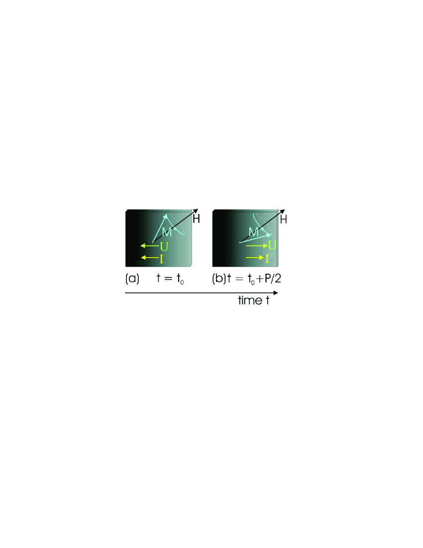
Figure 1: (Color online). Mechanism of the AMR-induced microwave photovoltage: $\mathbf{M}$ precesses (period P) in phase with the rf current $\mathbf{I}$. (a) $\mathbf{M}$ lying almost perpendicular to $\mathbf{I}$ results in low AMR. (b) $\mathbf{M}$ lying almost parallel to $\mathbf{I}$ results in high AMR. The time average voltage $\mathbf{U}$ becomes non-zero.

The second effect we investigate which is also based on AMR spin-charge coupling is the microwave photoresistance $\Delta R_{MW}$. This has been reported recently Costache06 with the equilibrium magnetization $\mathbf{M}_{0}$ of a ferromagnetic stripe aligned to a dc current $\mathbf{I}_{0}$. Microwave induced precession then misalignes the dynamic magnetization $\mathbf{M}$ with respect to $\mathbf{I_{0}}$ and thus makes the AMR drop measurably. In this work we present results which also show that if $\mathbf{M}_{0}$ lies perpendicular to $\mathbf{I}_{0}$ the opposite effect takes place: Microwave induced precession causes $\mathbf{M}$ to leave its perpendicular position what increases the AMR (see figure 2).

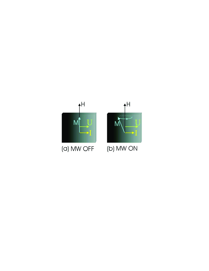
Figure 2: (Color online). Mechanism of the AMR-induced photoresistance: (a) Without microwaves (MW) $\mathbf{M}$ lies perpendicular to the dc current $\mathbf{I}$ and the AMR is minimal (b) With microwaves $\mathbf{M}$ precesses and is not perpendicular to $\mathbf{I}$ anymore. Consequently the AMR increases (higher voltage drop $\mathbf{U}$).

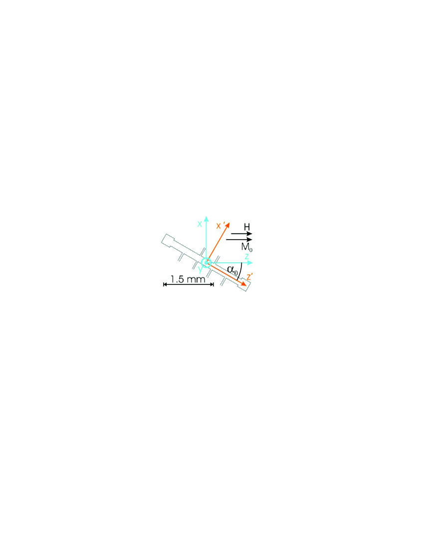
Figure 3: (Color online). (x,y,z) and (x^′,y,z^′) coordinate systems in front of a layout of our Permalloy film stripe ($200\times 2400\ \mu$m²) with 2 contacts and 6 side junctions.

After this qualitative introduction we want to go ahead with a quantitative description of the AMR induced microwave photovoltage and photoresistance. Therefore we define an orthogonal coordinate system (x,y,z) (see figure 3). The y-axis lies normal to the film plane and the z-axis is aligned with the magnetic field $\mathbf{H}$ and hence with the magnetization $\mathbf{M}$ which is always aligned with $\mathbf{H}$ in our measurements because of the sample being always magnetized to saturation.

Geometrically our samples are thin films patterned to stripe shape, so that $d\ll w\ll l$, where $d$, $w$ and $l$ are the thickness, width and length of the sample. We apply $\mathbf{H}$ always in the ferromagnetic film plane. For calculations based on the stripes geometry the coordinates $x^{\prime}$ and $z^{\prime}$ are defined. These lie in the film plane. $x^{\prime}$ is perpendicular and $z^{\prime}$ parallel to the stripe. The following coordinate transformation applies: $(x,y,z)=(x^{\prime}\cos(\alpha_{0})-z^{\prime}\sin(\alpha_{0}),y,z^{\prime}\cos(\alpha_{0})+x^{\prime}\sin(\alpha_{0}))$ where $\alpha_{0}$ is the angle between $\mathbf{H}$ and the stripe.

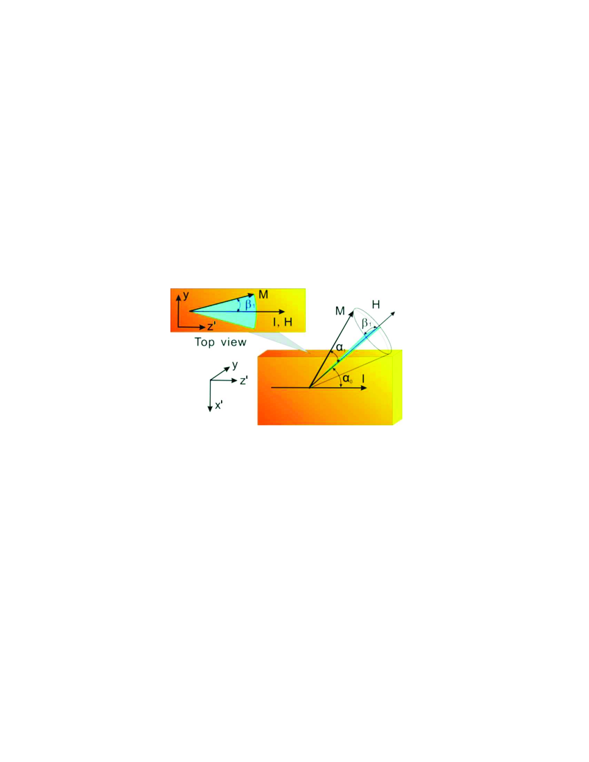
Figure 4: (Color online). Sketch of the magnetization precession. The magnetic field $\mathbf{H}$ encloses the angle $\alpha_{0}$ with the current $\mathbf{I}$. The magnetization oscillation towards $\mathbf{I}$ has the amplitude $\alpha_{1}$ and that perpendicular to $\mathbf{I}$: $\beta_{1}$.

For the microwave photovoltage and photoresistance the longitudinal resistance $R(t)=R_{0}+R_{A}\cos^{2}\theta(t)$ of the film stripe matters. It consists of the minimal longitudinal resistance $R_{0}$ and the additional resistance $R_{A}\cos^{2}\theta(t)$ from AMR. $\theta(t)$ is the angle between the $z^{\prime}$-axis (parallel to the stripe) and $\mathbf{M}$. $\mathbf{M}$ moves on a sphere with the radius $M_{0}$, which is the saturation magnetization of our sample. $\theta(t)$ can be decomposed into the angle $\alpha(t)$ in the ferromagnetic film plane and the out-of-plane angle $\beta(t)$ (see figure 4). Consequently:

$$\cos{\theta(t)}=\cos{\alpha(t)}\cos{\beta(t)}$$ (2)

Precession of the magnetization then yields oscillation of $\alpha(t)$, $\beta(t)$ and $\theta(t)$. In our geometry the equilibrium magnetization $\mathbf{M_{0}}$ encloses the in-plane angle $\alpha_{0}$ with the stripe. Hence in time average $<\beta(t)>\ =0$ and $<\alpha(t)>\ =\alpha_{0}$. In general the magnetization precession is elliptical. Its principle axis lie along the x- and y-axis and correspond to the amplitudes $\alpha_{1}$ and $\beta_{1}$ of the in- and out-of-plane angles $\alpha_{1}^{t}$ and $\beta_{1}^{t}$ of the rf magnetization: $\alpha(t)=\alpha_{0}+\alpha_{1}^{t}(t)=\alpha_{0}+\alpha_{1}\cos(\omega t-\psi)$ and $\beta(t)=\beta_{1}^{t}(t)=-\beta_{1}\sin(\omega t-\psi)$ (see figure 4). Using equation (2) we approximate $\cos^{2}\theta(t)$ to second order in $\alpha_{1}^{t}$ and $\beta_{1}^{t}$:

$$\cos^{2}\theta(t)\approx\cos^{2}\theta|_{\alpha_{1}^{t}=\beta_{1}^{t}=0}+\alpha_{1}^{t}\cdot\frac{d\cos^{2}\theta}{d\alpha_{1}^{t}}|_{\alpha_{1}^{t}=\beta_{1}^{t}=0}+0$$

$$+\frac{\alpha_{1}^{t2}}{2}\cdot\frac{d^{2}\cos^{2}\theta}{d\alpha_{1}^{t2}}|_{\alpha_{1}^{t}=\beta_{1}^{t}=0}+\frac{\beta_{1}^{t2}}{2}\cdot\frac{d^{2}\cos^{2}\theta}{d\beta_{1}^{t2}}|_{\alpha_{1}^{t}=\beta_{1}^{t}=0}$$ (3)

The first order in $\beta_{1}^{t}$ vanishes because it is proportional to $(\sin\beta)|_{\beta_{1}=0}=0$. It follows:

$$\cos^{2}\theta(t)\approx\cos^{2}\alpha_{0}-\alpha_{1}\cdot\sin 2\alpha_{0}\cos(\omega t-\psi)$$

$$-\alpha_{1}^{2}\cdot\cos 2\alpha_{0}\cos^{2}(\omega t-\psi)-\beta_{1}^{2}\cdot\cos^{2}\alpha_{0}\sin^{2}(\omega t-\psi)$$ (4)

This equation is now used to calculate the longitudinal stripe voltage. To consider the general case an externally applied dc current $I_{0}$ and a microwave induced rf current $I_{1}$, are included in $I(t)=I_{0}+I_{1}\cos(\omega t)$. It follows from equation (1):

$$U(t)=(R_{0}+R_{A}\cos^{2}\theta(t))\cdot(I_{0}+I_{1}\cos(\omega t))$$ (5)

Consequently $U(t)$ can be written as $U(t)=U_{0}+U_{1}\cos(\omega t-\psi_{1})+U_{2}\cos(2\omega t-\psi_{2})+U_{3}\cos(3\omega t-\psi_{3})$. For the photovoltage and photoresistance only the constant term $U_{0}$, which is equivalent to the time average voltage $\left<U(t)\right>$, matters. Combining equation (4) and (5), we find:

$$U_{0}=I_{0}(R_{0}+R_{A}\cos^{2}\alpha_{0})-I_{1}R_{A}\alpha_{1}\sin 2\alpha_{0}\cos(\psi)/2$$

$$-I_{0}(\alpha_{1}^{2}\cos 2\alpha_{0}+\beta_{1}^{2}\cos^{2}\alpha_{0})R_{A}/2$$ (6)

Note that: $\left<\sin^{2}(\omega t-\psi)\right>=\left<\cos^{2}(\omega t-\psi)\right>=1/2$, and $\left<\cos\omega t\cos(\omega t-\psi)\right>=\cos(\psi)/2$. The first term in equation (6) is independent of the rf quantities $I_{1}$, $\alpha_{1}$ and $\beta_{1}$ and represents the static voltage drop of $I_{0}$. The second term is the microwave photovoltage $U_{MW}$. It shows no impact from the dc current $I_{0}$. The third term represents the microwave photoresistance $\Delta R_{MW}$. It is proportional to $I_{0}$ and depends on the microwave quantities $\alpha_{1}$ and $\beta_{1}$. By the way: It can be seen now that the rf resistance amplitude $R^{1}$ used in the beginning of this paragraph corresponds to: $R^{1}=R_{A}\alpha_{1}\sin 2\alpha_{0}$.

To analyze the magnetization’s angle oscillation amplitudes $\alpha_{1}$ and $\beta_{1}$ it is necessary to express them by means of the corresponding rf magnetization $\Re(\mathbf{m}e^{-i\omega t})$. $\mathbf{m}$ is the complex rf magnetization amplitude. Its phase is defined with respect to $I_{1}$, so that $\Re(m_{x}e^{-i\omega t})$ is in phase with $I_{1}\cos\omega t$ at the FMR. Because $\mathbf{M}=\mathbf{M_{0}}+\mathbf{m}$, $\mathbf{m}=(m_{x},m_{y},0)$ can (in first order approximation) only lie perpendicular to $\mathbf{M}_{0}$ because $\mathbf{M}$ and $\mathbf{M_{0}}$ have the same length ($M_{0}$). Hence $|m_{x}|/M_{0}=\sin\alpha_{1}\approx\alpha_{1}$ and $|m_{y}|/M_{0}=\sin\beta_{1}\approx\beta_{1}$ for $\alpha_{1},\beta_{1}\ll 90^{\circ}$.

The microwave photovoltage and photoresistance appear whenever magnetization precession is excited. This means if the microwaves are in resonance with the FMR, with standing exchange spin waves perpendicular to the film Moller ; GuiHu ; Gui2 or with magnetostatic modes Gui2 . In this article we will analyze the FMR induced microwave photoresistance and photovoltage.

II.2 MAGNETIZATION DYNAMICS

To understand the impact of the applied rf magnetic field $\Re(\mathbf{h}e^{-i\omega t})$ on the microwave photovoltage and photoresistance the effective susceptibilities $\chi_{xx}$, $\chi_{xy}$ and $\chi_{yy}$, which link $\mathbf{m}e^{-i\omega t}$ inside the sample with the complex external rf magnetic field $\mathbf{h}e^{-i\omega t}=(h_{x},h_{y},h_{z})e^{-i\omega t}$ outside the sample, have to be calculated. Here $\psi$ is encoded in the complex phase of $\mathbf{m}$.

The susceptibility inside the sample (magnetic field $\mathbf{h^{in}}e^{-i\omega t}=(h_{x}^{in},h_{y}^{in},h_{z}^{in})e^{-i\omega t}$) is determined by the Polder tensorPolder $\hat{\chi}$ (received from solving the Landau-Liftshitz-Gilbert equation LLG ):

$$\mathbf{m}=\hat{\chi}\mathbf{h^{in}}=\left(\begin{array}[]{ccc}\chi_{L}&i\chi_{T}&0\\ -i\chi_{T}&\chi_{L}&0\\ 0&0&0\end{array}\right)\mathbf{h^{in}}$$ (7)

with

$$\chi_{L}=\frac{\omega_{M}\omega_{r}}{\omega_{r}^{2}-\omega^{2}},\ \chi_{T}=\frac{\omega\omega_{M}}{\omega_{r}^{2}-\omega^{2}}$$

where $\omega_{M}=\gamma M_{0}$ with the gyromagnetic ratio $\gamma\approx\mu_{0}\cdot e/m=2\pi\mu_{0}\cdot 28$ GHz/T (electron charge $e$ and mass $m_{e}$) and $\omega_{r}=\gamma H$ without damping. Approximation of our sample as a 2 dimensional film results in the boundary conditions that $h_{x}$ and $b_{y}$ are continuous at the film surface meaning $h_{x}=h_{x}^{in}$ and $b_{y}=\mu_{0}h_{y}=\mu_{0}((1+\chi_{L})h_{y}^{in}-i\chi_{T}h_{x}^{in})$. Hence:

$$\mathbf{m}=\left(\begin{array}[]{ccc}\chi_{xx}&i\chi_{xy}&0\\ -i\chi_{xy}&\chi_{yy}&0\\ 0&0&0\end{array}\right)\mathbf{h}$$ (8)

with

$$\chi_{xx}=\frac{\omega_{r}\omega_{M}+{\omega_{M}}^{2}}{\omega_{r}\left(\omega_{r}+\omega_{M}\right)-\omega^{2}}$$

$$\ \chi_{xy}=\frac{\omega\omega_{M}}{\omega_{r}\left(\omega_{r}+\omega_{M}\right)-\omega^{2}}$$

$$\chi_{yy}=\frac{\omega_{r}\omega_{M}}{\omega_{r}\left(\omega_{r}+\omega_{M}\right)-\omega^{2}}$$

$\chi_{xx}$ is identical to the susceptibility describing the propagation of microwaves in an unlimited ferromagnetic medium in Voigt geometry Camley (propagation perpendicular to $\mathbf{M}_{0}$). $\chi_{xx}$, $\chi_{xy}$ and $\chi_{yy}$ have the same denominator, which becomes resonant (maximal) when $\omega=\sqrt{\omega_{r}^{2}+\omega_{r}\omega_{M}}$. This is in accordance with the FMR frequency of the Kittel formula for in-plane magnetized infinite ferromagnetic films Kittel .

This relatively simple behavior is due to the assumption, that $\mathbf{h^{in}}$ is constant within the film stripe. This assumption is only valid if the skin depth Guru $\delta$ of the microwaves in the sample is much larger than the sample thickness. During our measurements we fix the microwave frequency $f$ and sweep the magnetic field $H$. Consequently we find the FMR magnetic field $H_{0}$ with

$$\omega^{2}=\gamma^{2}(H_{0}^{2}+H_{0}M_{0})$$ (9)

and

$$H_{0}=\sqrt{M_{0}^{2}/4+\omega^{2}/\gamma^{2}}-M_{0}/2$$ (10)

Now we introduce Gilbert dampingGilbert $\alpha_{G}$ by setting $\omega_{r}:=\omega_{0}-i\alpha_{G}\omega$ with now $\omega_{0}=\gamma H$ instead of $\omega_{r}=\gamma H$. We separate the real and imaginary part of $\chi_{xx}$, $\chi_{xy}$ and $\chi_{yy}$:

$$\chi_{xx}=(\omega_{r}\omega_{M}+{\omega_{M}}^{2})\cdot F$$

$$\chi_{xy}=\omega\omega_{M}\cdot F$$ (11)

$$\chi_{yy}=\omega_{r}\omega_{M}\cdot F$$

with

$$F=\frac{\omega_{0}(\omega_{0}+\omega_{M})-\alpha_{G}^{2}\omega^{2}-\omega^{2}+i\alpha_{G}\omega(2\omega_{0}+\omega_{M})}{(\omega_{0}(\omega_{0}+\omega_{M})-\alpha_{G}^{2}\omega^{2}-\omega^{2})^{2}+\alpha_{G}^{2}\omega^{2}(2\omega_{0}+\omega_{M})^{2}}$$

$$\approx\frac{(H+H_{0}+M_{0})(H-H_{0})+i(2H+M_{0})\alpha_{G}\omega/\gamma}{((H+H_{0}+M_{0})^{2}(H-H_{0})^{2}+(2H+M_{0})^{2}\alpha_{G}^{2}\omega^{2}/\gamma^{2}}$$

The approximation was done by neglecting the $\alpha_{G}^{2}\omega^{2}$ correction to the resonance frequency $\omega^{2}=\omega_{0}(\omega_{0}+\omega_{M})-\alpha_{G}^{2}\omega^{2}\approx\omega_{0}(\omega_{0}+\omega_{M})$ what is possible if $\alpha_{G}\ll 1$. Hence:

$$\chi_{xx,xy,yy}\approx A_{xx,xy,yy}\cdot\frac{\Delta H(H-H_{0})+i\Delta H^{2}}{(H-H_{0})^{2}+\Delta H^{2}}$$ (12)

with $\Delta H=((2H+M_{0})/(H+H_{0}+M_{0}))\cdot\alpha_{G}\omega/\gamma$. This can be approximated as $\Delta H\approx\alpha_{G}\omega/\gamma$ if $|H-H_{0}|\ll H_{0}$. $A_{xx}$, $A_{xy}$ and $A_{yy}$ determine the scalar amplitude of $\chi_{xx}$, $\chi_{xy}$ and $\chi_{yy}$.

To analyze the FMR line shape in the following, we will call the Lorentz line shape which is proportional to $\Delta H/((H-H_{0})^{2}-\Delta H^{2})$ symmetric Lorentz line shape and the line shape proportional to $(H-H_{0})/((H-H_{0})^{2}-\Delta H^{2})$ antisymmetric Lorentz line shape. A linear combination of both will be called asymmetric Lorentz line shape. $|H-H_{0}|\ll H_{0}$ allows us to approximate:

$$A_{xx}\approx\frac{\gamma(H_{0}M_{0}+M_{0}^{2})}{\alpha_{G}\omega(2H_{0}+M_{0})}$$

$$A_{xy}\approx\frac{M_{0}}{\alpha_{G}(2H_{0}+M_{0})}$$ (13)

$$A_{yy}\approx\frac{\gamma H_{0}M_{0}}{\alpha_{G}\omega(2H_{0}+M_{0})}$$

These are scalars which are independent of the DC magnetic field $H$ and hence characteristic for the sample at fixed frequency. Indeed the assumption of Gilbert damping is not essential for the derivation of equation (13). In the event of a different kind of damping, $\Delta H$ can also be directly input into equation (13) replacing $\alpha_{G}\omega$. However because of the commonness of Gilbert damping, its usage here can provide a better feeling for the usual frequency dependence of $A_{xx,xy,yy}$. Going ahead, equation (8) becomes:

$$\mathbf{m}\approx\frac{\Delta H(H-H_{0})+i\Delta H^{2}}{(H-H_{0})^{2}+\Delta H^{2}}\left(\begin{array}[]{ccc}A_{xx}&iA_{xy}&0\\ -iA_{xy}&A_{yy}&0\\ 0&0&0\end{array}\right)\mathbf{h}$$ (17)

The $H$-field dependencies has Lorentz line shape with antisymmetric (dispersive) real and symmetric (absorptive) imaginary part, the amplitudes $A_{xx}$, $\pm iA_{xy}$ and $A_{yy}$ respectively and the width $\Delta H$. Note that $A_{xx}A_{yy}\approx A_{xy}^{2}$ for $|H-H_{0}|\ll H_{0}$. Consequently the susceptibility amplitude tensor can be simplified to:

$$\left(\begin{array}[]{ccc}A_{xx}&iA_{xy}&0\\ -iA_{xy}&A_{yy}&0\\ 0&0&0\end{array}\right)\mathbf{h}\approx\left(\begin{array}[]{c}\sqrt{A_{xx}}\\ -i\sqrt{A_{yy}}\\ 0\end{array}\right)\left[\left(\begin{array}[]{c}\sqrt{A_{xx}}\\ i\sqrt{A_{yy}}\\ 0\end{array}\right)\cdot\mathbf{h}\right]$$ (27)

and equation (17) becomes:

$$\mathbf{m}=\frac{\gamma M_{0}}{\alpha_{G}\omega(2H_{0}+M_{0})}\frac{\Delta H(H-H_{0})+i\Delta H^{2}}{(H-H_{0})^{2}+\Delta H^{2}}$$

$$\cdot\left(\begin{array}[]{c}\sqrt{1+M_{0}/H_{0}}\\ -i\\ 0\end{array}\right)\left(\left(\begin{array}[]{c}\sqrt{1+M_{0}/H_{0}}\\ i\\ 0\end{array}\right)\cdot\mathbf{h}\right)$$ (34)

It is visible that the ellipcity of $\mathbf{m}$ is independent of the exciting magnetic field $\mathbf{h}$. Only the amplitude and phase of $\mathbf{m}$ are defined by $\mathbf{h}$. The reason is the weak Gilbert damping $\alpha_{G}$ for which much energy needs to be stored in the magnetization precession to have a compensating dissipation. Hence little energy input and impact from $\mathbf{h}$ appears.

From equation (34) follows that $m_{x}$ and $m_{y}$ have cardinally the ratio:

$$m_{x}/m_{y}=i\sqrt{1+M_{0}/H_{0}}$$ (35)

Therefore $m_{y}$ vanishes for $\omega\rightarrow 0$ and $m_{x}=im_{y}$ for $\omega\rightarrow\infty$. This means that the precession of $\mathbf{M}$ is elliptical and becoming more circular for high frequencies and more linear (along the x-axis) for low frequencies. This description applies for the case of an in-plane magnetized ferromagnetic film. However in the case that the sample has circular symmetry with respect to the magnetization direction (e.g. in a perpendicular magnetized disc or infinite filmGuiHu ; Gui2 ): $\alpha_{1}=\beta_{1}$. This is the same as in the case that $\omega\rightarrow\infty$ . Only in these cases the magnetization precession can be described in terms of one precession cone angle Costache06 . Otherwise distinct attention has to be paid to $\alpha_{1}$ and $\beta_{1}$ (see III.2). Additionally it can be seen in equation (34) that $\overline{m_{y}}/\overline{m_{x}}$ is also the ratio of the coupling strength of $\mathbf{m}$ to $h_{y}$ and $h_{x}$ respectively.

II.3 MICROWAVE PHOTORESISTANCE

The microwave photoresistance $\Delta R_{MW}$ can be deduced from equation (6). First the microwave photovoltage is excluded by setting the rf current $I_{1}=0$. Then we only regard the microwave power dependent terms which depend on $\alpha_{1}$ and $\beta_{1}$:

$$\Delta R_{MW}=(U_{0}|_{I_{1}=0}-U_{0}|_{I_{1}=0,\alpha_{1}=0,\beta_{1}=0})/I_{0}$$

$$=R_{A}(-\alpha_{1}^{2}\cos 2\alpha_{0}-\beta_{1}^{2}\cos^{2}\alpha_{0})/2$$ (36)

If the magnetization lies parallel or antiparallel to the dc current vector $\mathbf{I_{0}}$ along the stripe ($\alpha_{0}=0^{\circ}$ or $\alpha_{0}=180^{\circ}$) the AMR is maximal. In this case magnetization oscillation ($\alpha_{1}$ and $\beta_{1}$) reduces (-$\cos 2\alpha_{0}=-1$) the AMR by $\Delta R_{MW}=-(\alpha_{1}^{2}+\beta_{1}^{2})R_{A}/2$ (negative photoresistance). In contrast if the magnetization lies perpendicular to $\mathbf{I}_{0}$ ($\alpha_{0}=90^{\circ}$, see figure 2) the resistance is minimal. In this case magnetization oscillation corresponding to $\alpha_{1}$ will increase ($-\cos 2\alpha_{0}=+1$) the AMR (positive photoresistance) by $\Delta R_{MW}=+\ \alpha_{1}^{2}\cdot R_{A}/2$ (oscillations corresponding to $\beta_{1}$ leave $\theta(t)$ constant in this case and do not change the AMR).

The next step is to calculate $\alpha_{1}$ and $\beta_{1}$. The dc magnetic field dependence of $\alpha_{1}=|m_{x}|/M_{0}=|\chi_{xx}h_{x}+i\chi_{xy}h_{y}|/M_{0}$ and $\beta_{1}=|m_{y}|/M_{0}=|-i\chi_{xy}h_{x}+\chi_{yy}h_{y}|/M_{0}$ is proportional to that of $|\chi_{xx}|$, $|\chi_{xy}|$ and $|\chi_{yy}|$ given in equation (12) (imaginary symmetric and real antisymmetric Lorentz line shape). Squaring this results in symmetric Lorentz line shape:

$$\alpha_{1}^{2}\propto\beta_{1}^{2}\propto\left|\frac{\Delta H(H-H_{0})+i\Delta H^{2}}{(H-H_{0})^{2}+\Delta H^{2}}\right|^{2}=\frac{\Delta H^{2}}{(H-H_{0})^{2}+\Delta H^{2}}$$

Hence:

$$\alpha_{1}^{2}=\frac{|A_{xx}h_{x}+iA_{xy}h_{y}|^{2}}{M_{0}^{2}}\cdot\frac{\Delta H^{2}}{(H-H_{0})^{2}+\Delta H^{2}}$$

$$\beta_{1}^{2}=\frac{|A_{yy}h_{y}-iA_{xy}h_{x}|^{2}}{M_{0}^{2}}\cdot\frac{\Delta H^{2}}{(H-H_{0})^{2}+\Delta H^{2}}$$ (37)

Using equation (34) and (37), equation (36) transforms to:

$$\Delta R_{MW}=\frac{R_{A}}{(\alpha_{G}\omega/\gamma)^{2}(2H_{0}+M_{0})^{2}}$$

$$\cdot(-(H_{0}+M_{0})\cos 2\alpha_{0}-H_{0}\cos^{2}\alpha_{0})$$ (38)

$$\cdot\frac{\Delta H^{2}}{(H-H_{0})^{2}+\Delta H^{2}}\cdot|h_{x}\sqrt{H_{0}+M_{0}}+ih_{y}\sqrt{H_{0}}|^{2}$$

The strength of the microwave photoresistance is proportional to $1/\alpha_{G}^{2}$. Weak damping (small $\alpha_{G}$) is therefore critical for a signal strength sufficient for detection. The magnetic field dependence shows symmetric Lorentz line shape.

The dependence of $\Delta R_{MW}$ on $\alpha_{0}$ in equation (II.3) reveals a sign change and hence vanishing of the photoresistance at

$$\cos^{2}\alpha_{0}=\frac{1}{2}\left(1-\frac{H_{0}}{3H_{0}+2M_{0}}\right)$$ (39)

This means that the angle at which the photoresistance vanishes shifts from $\alpha_{0}=\pm 45^{\circ}$ and $\alpha_{0}=\pm 135^{\circ}$ (for $\omega\rightarrow 0$) to $\alpha_{0}=\pm 54.7^{\circ}$ and $\alpha_{0}=\pm 125.3^{\circ}$ respectively (for $\omega\rightarrow\infty$) when increasing $\omega$. The reason for this frequency dependence is the frequency dependence of the ellipcity of $\mathbf{m}$ described at the end of II.2.

II.4 MICROWAVE PHOTOVOLTAGE

The most obvious difference in appearence between the microwave photoresistance discussed in paragraph II.3 and the microwave photovoltage discussed in this paragraph is that the photoresistance is proportional to the square of the rf magnetization (see equation (36), $\alpha_{1}^{2}\approx|m_{x}|^{2}/M_{0}^{2}$ and $\beta_{1}^{2}\approx|m_{y}|^{2}/M_{0}^{2}$) while the photovoltage $U_{MW}$ is proportional to the product of the rf magnetization and the rf current. Consequently the photovoltage has a very different line shape: While the rf magnetization depends with Lorentz line shape on $H$ (see equation (12)), $I_{1}$ is independent of $H$. The line shape is hence determined by the phase difference $\psi$ between the rf magnetization component $\Re(m_{x}e^{-i\omega t})$ and the rf current $I_{1}\cos\omega t$. This effect does not play a role in the case of photoresistance because there only one phase matters namely that of the rf magnetization. In contrast in photovoltage measurements a linear combination of symmetric and antisymmetric Lorentz line shapes is found. This will be discussed in detail in the following.

To isolate the microwave photovoltage in equation (6) the dc current $I_{0}$ is set to 0:

$$U_{MW}=U_{0}|_{I_{0}=0}=-I_{1}\alpha_{1}\frac{R_{A}\sin 2\alpha_{0}\cos\psi}{2}$$ (40)

From equation (8) we follow:

$$\alpha_{1}\cos\psi=\Re(m_{x})=\Re(\chi_{xx}h_{x}+i\chi_{xy}h_{y})$$ (41)

We split $h_{x}=h_{x}^{r}+ih_{x}^{i}$ and $h_{y}=h_{y}^{r}+ih_{y}^{i}$ into real ($h_{x}^{r}$, $h_{y}^{r}$) and imaginary ($h_{x}^{i}$, $h_{y}^{i}$) part. This enables us to isolate the real part in equation (40) using equation (17):

$$U_{MW}=\frac{I_{1}R_{A}\sin 2\alpha_{0}}{2M_{0}}\cdot\{\frac{\left(A_{xy}h^{r}_{y}+A_{xx}h^{i}_{x}\right)\Delta H^{2}}{(H-H_{0})^{2}+\Delta H^{2}}$$

$$+\frac{\left(A_{xy}h^{i}_{y}-A_{xx}h^{r}_{x}\right)\Delta H(H-H_{0})}{(H-H_{0})^{2}+\Delta H^{2}}\}$$ (42)

Conclusively in contrast to the microwave photoresistance ($\Delta R_{MW}\propto 1/\alpha_{G}^{2}$, see equation (II.3)) the photovoltage is only proportional to $1/\alpha_{G}\propto A_{xx,xy,yy}$. Thus good damping is less important for its detectionEgan .

To understand the measurement results it will be necessary to transform the coordinate system of equation (II.4) to (x’,y,z’). In this coordinate system the rf magnetic field $\mathbf{h}$ is constant during rotation as described in equation (III.3).

To better understand the photovoltage line shape we have a closer look on $\psi$: When sweeping $H$ the rf magnetization phase is shifted by $\psi_{m}$ with respect to the resonance case ($H=H_{0}$). The rf current has a constant phase $\psi_{I}$ which is defined with respect to the magnetization’s phase at resonance. The impact of the dc magnetic field $H$ on the rf current ($I_{1}$, $\psi_{I}$) via the FMR is believed to be negligible:

$$\cos\psi=\cos(\psi_{m}-\psi_{I})=\cos\psi_{m}\cos\psi_{I}+\sin\psi_{m}\sin\psi_{I}$$ (43)

$\psi$ is determined by the (complex) phase of $\chi_{xx}$, $\chi_{xy}$ and $\chi_{yy}$ with respect to the resonance case ($\Re(\chi_{xy,yy})=0$ at $H=H_{0}$) during magnetic field sweep (asymmetric Lorentz line shape, see equation (12)):

$$\tan\psi_{m}=\frac{\Im\left(\frac{\Delta H(H-H_{0})+i\Delta H^{2}}{(H-H_{0})^{2}+\Delta H^{2}}/i\right)}{\Re\left(\frac{\Delta H(H-H_{0})+i\Delta H^{2}}{(H-H_{0})^{2}+\Delta H^{2}}/i\right)}=\frac{H_{0}-H}{\Delta H}$$ (44)

It should be noted that according to the Landau-Liftshitz equation LLG $\mathbf{h}$ applies a torque on the magnetization and hence excites $\mathbf{m}^{t}$ transversal. That is why at resonance $m_{x}$ shows a phase shift of $90^{\circ}$ with respect to $h_{x}$. Consequently in equation (44) division by $i$ is necessary ($\chi_{xx}$ and $\chi_{xy}$ become imaginary at resonance).

Equation (44) means that in case that the applied microwave frequency is higher than the FMR frequency ($H_{0}>H$) $\psi_{m}>0$ (note that $\mathbf{m}^{t}=\mathbf{m}e^{-i\omega t}$), $\mathbf{m}^{t}$ is delayed with respect to the resonant case. The other way around ($H_{0}<H$) the FMR frequency is higher than that of the applied microwave field and $\mathbf{m}^{t}$ is running ahead compared to the resonance case. Using equation (44) we find:

$$\cos\psi_{m}=\frac{\Delta H}{\sqrt{(H-H_{0})^{2}+\Delta H^{2}}}$$

(45)

Inserting equation (37), (43), (44) and (45) into (40) gives:

$$U_{MW}=-\frac{R_{A}I_{1}\sin 2\alpha_{0}}{2}\cdot\frac{|A_{xx}h_{x}+iA_{xy}h_{y}|}{M_{0}}$$

$$\cdot\left(\frac{\Delta H^{2}\cos\psi_{I}}{(H-H_{0})^{2}+\Delta H^{2}}-\frac{(H-H_{0})\Delta H\sin\psi_{I}}{(H-H_{0})^{2}+\Delta H^{2}}\right)$$ (46)

The dependence on $H$ takes the form of a linear combination of symmetric and antisymmetric Lorentz line shape with the ratio 1 :$\ \tan\psi_{I}$. The symmetric line shape contribution ($\propto\Delta H$) arises from the rf current contribution that is in phase with the rf magnetization at FMR and the antisymmetric from that out-of-phase. This gives a nice impression of the phase $\psi_{I}$ of the rf current determining the line shape of the FMR.

II.5 VECTORIAL DESCRIPTION OF THE PHOTOVOLTAGE

To complete the discussion of the microwave photovoltage we want to return to the approach used by JuretschkeJuretschke to demonstrate that it is consistent with the description above. In II.1 we started with Ohm’s law (scalar equation (1)). There we integrate an angle- and time-dependent resistance. Here we want to start with the vectorial notation of Ohm’s law used in Juretschke’s publication (equation (1)Juretschke ). This integrates AMR and anomalous Hall effect AHE. $\rho$ is the resistivity of the sample and $\Delta\rho$ that additionally arising from AMR. $R_{H}$ is the anomalous Hall effect constant:

$$\mathbf{E}=\rho\mathbf{J}+(\Delta\rho\mathbf{M}^{2})(\mathbf{J}\cdot\mathbf{M})\mathbf{M}-R_{H}\mathbf{J}\times\mathbf{M}$$ (47)

We split $\mathbf{M}=\mathbf{M_{0}}+\mathbf{m}^{t}$ and the current density $\mathbf{J}=\mathbf{J_{0}}+\mathbf{j}^{t}$ into their dc ($\mathbf{M}_{0}$ and $\mathbf{J}_{0}$) and rf contributions ($\mathbf{m}^{t}=\Re(\mathbf{m}e^{-i\omega t})$ and $\mathbf{j}^{t}=\mathbf{j}\cos\omega t$). Constance of $|\mathbf{M}|$ allows $\mathbf{m}^{t}=(m^{t}_{x},m^{t}_{y},0)$ in first order approximation only to lie perpendicular to $\mathbf{M_{0}}=(0,0,M_{0})$. To select the photovoltage we set $\mathbf{J}_{0}=0$ and approximate equation (47) to second order in $\mathbf{j}^{t}$ and $\mathbf{m}^{t}$. The terms of zeroth order in both $\mathbf{j}^{t}$ and $\mathbf{m}^{t}$ represent the sample resistance without microwave exposure and are not discussed here. The terms of first order in either $\mathbf{j}^{t}$ or $\mathbf{m}^{t}$ (but not both) have zero time average and do not contribute to the microwave induced dc electric field $\mathbf{E}_{MW}$. Only the terms that are simultaneously of first order in $\mathbf{j}^{t}$ and $\mathbf{m}^{t}$ contribute to $\mathbf{E}_{MW}$ (compare equation (4) from JuretschkeJuretschke ):

$$\mathbf{E}_{MW}=\frac{\Delta\rho}{{M_{0}}^{2}}\left<\left(\mathbf{j}^{t}\mathbf{m}^{t}\right)\mathbf{M_{0}}+\left(\mathbf{j}^{t}\mathbf{M_{0}}\right)\mathbf{m}^{t}\right>-R_{H}\left<\mathbf{j}^{t}\times\mathbf{m}^{t}\right>$$ (48)

The $\Delta\rho$ dependent term represents the photovoltage contribution arising from AMR and the $R_{H}$ dependent term that arising from AHE. Note that a second order of $\mathbf{m}^{t}$ appears when applying a dc current $\mathbf{J_{0}}\not=0$. It represents the photoresistance discussed in II.3. However it we will not be discussed here.

In the following we will calculate the photovoltage in our Permalloy film stripe considering its geometry which fixes the current direction. $\mathbf{j}^{t}=j^{t}_{z\prime}\mathbf{z\prime}$ along the stripe ($\mathbf{z\prime}$ is the unit vector along the Permalloy stripe). The small dimensions perpendicular to the stripe ($\ll L$) will prevent the formation of a perpendicular rf current. A similar approximation of a metal grating forming a linear polarizer has been considered previouslyGui . The photovoltage $U_{MW}$ is also measured along the stripe (length vector $\mathbf{L}=\mathbf{z^{\prime}}\cdot 2.4$ mm). When fluctuations of $\mathbf{E}_{MW}$ along the stripe are neglected considering the large microwave wavelength, $\lambda\approx 20$ mm $\gg 2.4$ mm $=L$, we find $U_{MW}$ by multiplying $\mathbf{E}_{MW}$ with $\mathbf{L}$:

$$U_{MW}=\int_{0}^{L}\mathbf{E_{MW}}\mathbf{dz^{\prime}}\approx\mathbf{E}_{MW}\cdot\mathbf{L}=$$

$$\frac{\Delta\rho L}{{M_{0}}^{2}}\left<j^{t}_{z\prime}\left(\mathbf{z\prime}\mathbf{m}^{t}\right)\left(\mathbf{M_{0}}\mathbf{z\prime}\right)+j^{t}_{z\prime}\left(\mathbf{z\prime}\mathbf{M_{0}}\right)\left(\mathbf{m}^{t}\mathbf{z\prime}\right)\right>-0$$ (49)

$$=\frac{\Delta\rho L}{M_{0}}\left<j^{t}_{z\prime}m^{t}_{x}\right>\sin(2\alpha_{0})$$

This is equivalent to equation (40) which can be verified by replacing $\Delta\rho j^{t}_{z\prime}L=R_{A}I_{1}\cos(\omega t)$ and $m_{x}^{t}=\alpha_{1}M_{0}\cos(\omega t-\psi)$. Time averaging results in the additional factor $\cos(\psi)/2$.

As discussed in II.6 the contribution belonging to the anomalous Hall effect has no impact in this geometry because it can only generate a photovoltage perpendicular to the rf current i.e. perpendicular to the stripe.

Comparing our results to those of Juretschke and EganJuretschke ; Egan , we note that an equation similar to (II.5) has been derived in the formula for $e_{y0}$ in equation (31) in Juretschke’s publication Juretschke . There the photovoltage is measured parallel to the rf current as done in our stripe. However it has to be noted that the coordinate system is defined differently. The major difference compared to our system is that we use a stripe shaped film to lithographically define the direction of the rf current $I_{1}$, while the direction of $\mathbf{h}$ is left arbitrary. In contrast to that Juretschke and EganJuretschke ; Egan define the direction of the rf magnetic field and rf current by means of their microwave setup. In equation (31) ($e_{y0}$) from Juretschke Juretschke this results in the additional factor $\cos\theta$ (which is equivalent to $\cos\alpha_{0}$ in our work) compared to equation (II.5). This arises from the definition of $\mathbf{h}$ fixed parallel to the rf current (compare equation (III.3)).

II.6 OTHER MAGNETORESISTIVE EFFECTS THAT COUPLE SPIN AND CHARGE CURRENT

In this section we present other magnetoresistive effects which can generate photovoltage and photoresistance like the AMR. This selection gives a broader view on the range of effects for which the photovoltage and photoresistance can be discussed in terms of the analysis presented in this work. In principle every magnetoresistive effect can modulate the sample resistance and thus rectify some of the rf current to photovoltage.

One magnetoresistive effect is the anomalous Hall effect AHE in ferromagnetic metals that was (together with the AMR) the basis for the discussion of Juretschke Juretschke . There a current with perpendicular magnetization generates a voltage perpendicular to both. Under microwave exposure this alternates with the microwave frequency but in an asymmetric way due to the modulated AHE arising from magnetization precession. The asymmetric voltage has a dc contribution (photovoltage)Egan which can be measured using a 2 dimensional ferromagnetic film with the magnetization neither parallel nor perpendicular to it. The photovoltage induced by AHE appears in the film plane perpendicular to the rf current and is smallMoller for Permalloy (Ni₈₀Fe₂₀). Also a photoresistive effect which alters the AHE can be expected if the magnetization lies out-of-plane.

Other examples for magnetoresistive effects are GMR and TMR structures which exhibit a photovoltage mechanism similar to that in AMR films. The difference is that there not the direction of the ferromagnetic layer magnetization with respect to the current matters. Effectively instead the direction of the magnetization $\mathbf{M}$ of one ferromagnetic layer with respect to that of another layer is decisive (see figure 5). Exciting the FMR in one layer yields again oscillation of the sample resistance $R(t)$ and thus gives the corresponding rf voltage $U(t)$ a non-zero time average (photovoltage) Tulapurkar ; Kupferschmidt . This is usually stronger than that from AMR films due to the generally higher relative strength of GMR and TMR compared to AMR.

It should be noted that in current studies of the microwave photovoltages effect in multilayer structures, the focus is on interfacial spin transfer effects Tulapurkar ; Sankey ; Azevedo ; Saitoh ; Costache ; Berger99 ; Brataas ; Wang ; Kupferschmidt . It remains an intriguing question whether interfacial spin transfer effects and the effect revealed in our approach based on phenomenological magnetoresistance might be unified by a consistent microscopic model, as Silsbee et al. have demonstrated for describing both bulk and interfacial spin transport under rf excitation Silsbee .

Multilayer structures also provide a nice example that photovoltage generation can also be reversed when the oscillating magnetoresistance, transforms a dc current into an rf voltage Kiselev , instead of transforming an rf current into a dc voltage (photovoltage). This gives a new kind of microwave source and seems - although weaker - also possible in AMR and AHE samples.

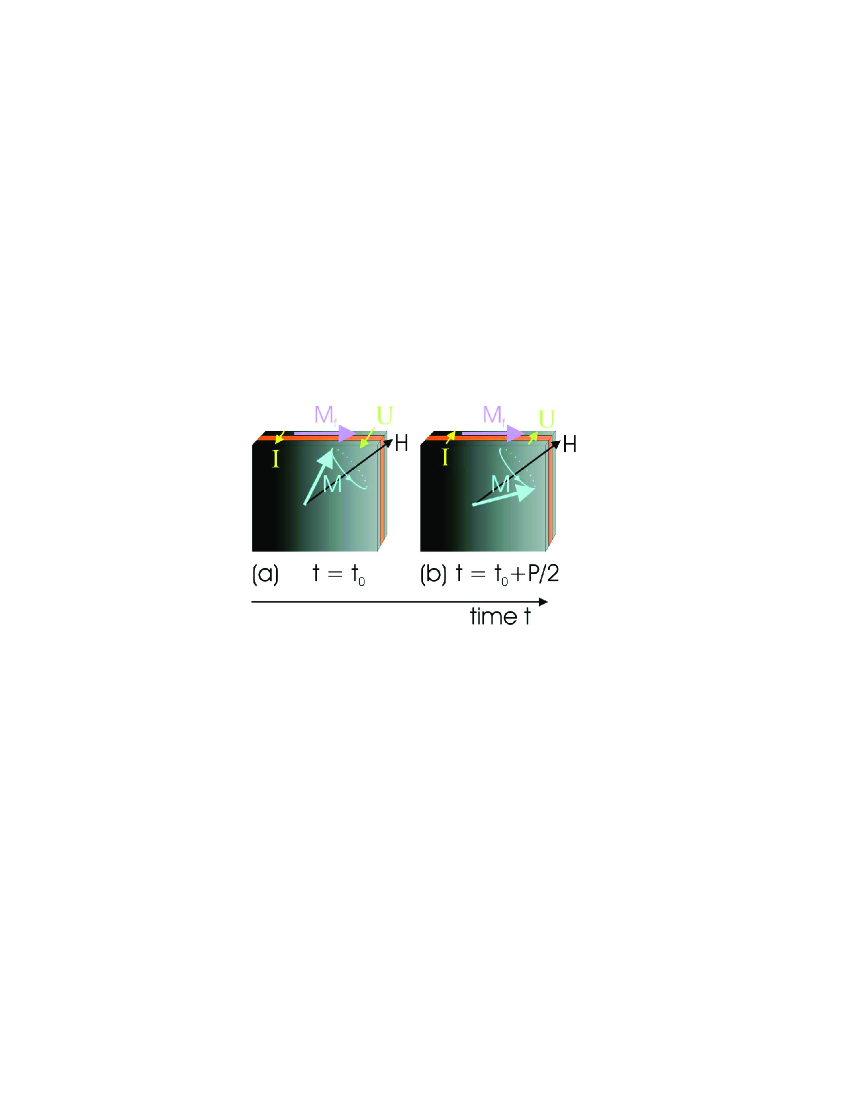
Figure 5: (Color online). Microwave photovoltage in a GMR/TMR-heterostructure (ferromagnetic($\mathbf{M}$)/non-ferromagnetic/ferromagnetic($\mathbf{M_{f}}$)): The dynamic magnetization $\mathbf{M}$ precesses (period P) in phase with the current $\mathbf{I}$. (a) $\mathbf{M}$ lies almost perpendicular to $\mathbf{M_{f}}$: high GMR/TMR. (b) $\mathbf{M}$ lies almost parallel to $\mathbf{M_{f}}$: low GMR/TMR $\Rightarrow$ Non-zero time average of the voltage $\mathbf{U}$.

It can be reasoned that like microwave photovoltage the microwave photoresistance can also be based on GMR or TMR instead of AMR: When aligning the 2 magnetizations of both ferromagnetic layers in a GMR or TMR structure microwave induced precession of one magnetization is expected to increase the GMR/TMR because of the arising misalignment with the other magnetization. With the magnetizations initially anti parallel the opposite effect, a microwave induced resistance decrease, is expected. Further work demonstrating these effects would be interesting.

III PHOTOVOLTAGE MEASUREMENTS

III.1 MEASUREMENT SETUP

The sample we use to investigate the microwave photovoltage consists of a thin (d = 49 nm) Permalloy (Ni 80%, Fe 20%) film stripe (200 $\mu$m wide and 2400 $\mu$m long) with 300$\times$300 $\mu$m² bond pads at both ends (see figure 3). These are connected via gold bonding wires and coaxial cables to a lock-in amplifier. For auxiliary measurements (e.g. Hall effect) 6 additional junctions are attached along the stripe (see figure 3).

The resistance of the film stripe is $R_{0}+R_{A}=85.0\ \Omega$ for parallel and $R_{0}=83.6\ \Omega$ for perpendicular magnetization. Hence the conductance is $\sigma=1/\rho=2.9\cdot 10^{6}\ \Omega^{-1}$m^-1 and the relative AMR is $\Delta\rho/\rho=1.7\ \%$. The absolute AMR is $R_{A}=1.4\ \Omega$. This is in good agreement with previous publications Gui ; GuiHu ; Gui2 .

The film is deposited on a 0.5 mm thick GaAs single crystal substrate, and patterned using photolithography and lift off techniques. The substrate is mounted on a 1 mm polyethylene print circuit board which is glued to a brass plate holding it in between the poles of an electromagnet. This provides the dc magnetic field $B=\mu_{0}H$ (maximal $\approx 1$ T). The sample is fixed 1 mm behind the end of a WR62 ($15.8\times 7.9$ mm) hollow brass waveguide which is mounted normal to the Permalloy film plane. The stripe is fixed along the narrow waveguide dimension. In the K_u band (12.4 - 18 GHz), that we use in our measurements, the WR62-waveguide only transmits the TE₀₁ mode Guru . The stripe was fixed with respect to the waveguide but was left rotatable with respect to $\mathbf{H}$. This allows the stripe to be parallel or perpendicular to $\mathbf{H}$, but keeps the magnetic field always in the film plane. A high precision angle readout was installed to indicate $\alpha_{0}$.

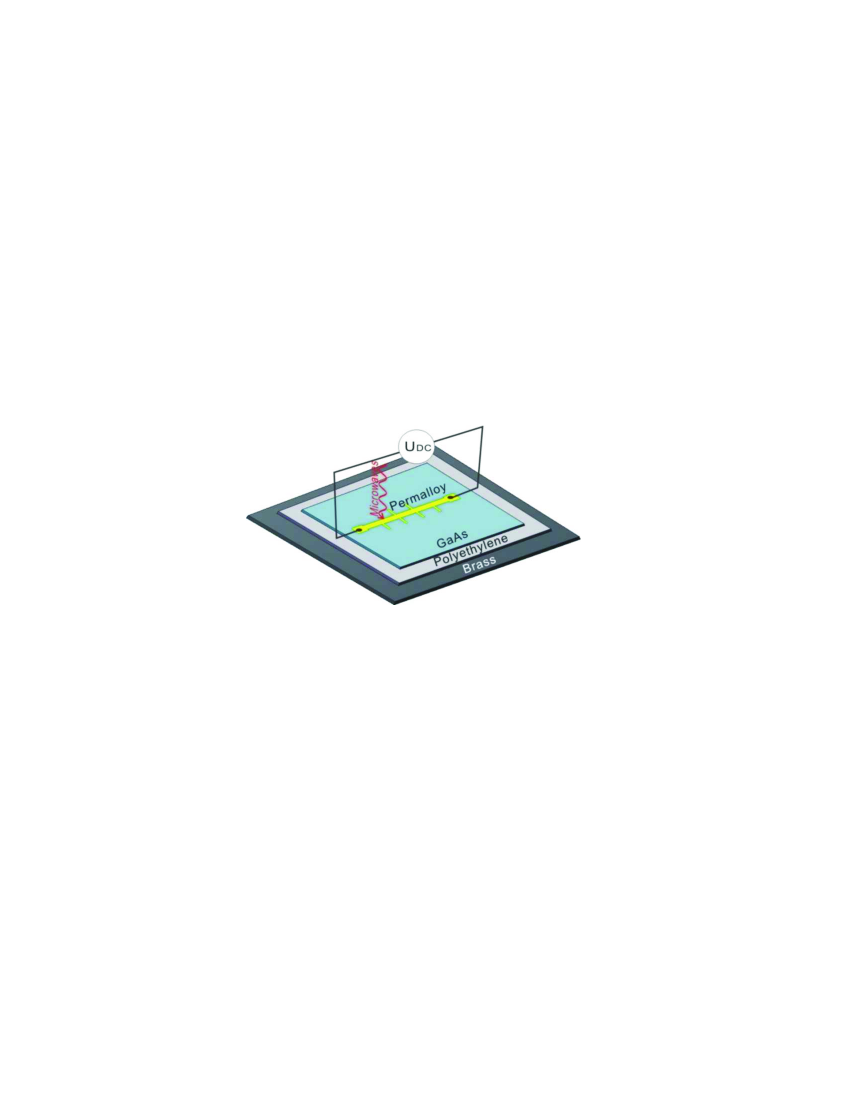
Figure 6: (Color online). Sketch of the measurement geometry. A 1 mm thick polyethylene plate is glued on a brass holder. On top of the polyethylene a GaAs substrate is glued. On the substrate the Permalloy (Py) stripe is defined. This is electrically wired to a voltage amplifier for photovoltage measurements. For photoresistance measurements an additional current source is connected parallel to the voltage amplifier, which is not shown explicitly here.

The waveguide is connected to an HP83624B microwave generator by a coaxial cable supplying frequencies of up to 20 GHz and a power of 200 mW. The power is however later significantly reduced by losses occurring within the coaxial cable, during the transfer to the hollow waveguide and by reflections at the end of the waveguide. Microwave photovoltage measurements are performed sweeping the magnetic field while fixing the microwave frequency. The sample is kept at room temperature.

To avoid external disturbances the photovoltage was detected using a lock-in technique: A low frequency (27.8 Hz) square wave signal is modulated on the microwave CW-output. The lock-in amplifier, connected to the Permalloy stripe, is triggered to the modulation frequency to measure the resulting square wave photovoltage across the sample. Instead of the photovoltage also the photocurrent can be measuredGuiHu . Its strength $I_{0}$ can be found when setting $U_{0}=0$ in equation (6) (instead of $I_{0}=0$).

III.2 FERROMAGNETIC RESONANCE

The measured photovoltage almost vanishes during most of the magnetic field sweep but shows one pronounced resonance of several $\mu$V. The strength and line shape of this resonance are strongly depending on $\alpha_{0}$ and will be discussed in 10. A line shape dependence of the photovoltage on the microwave frequency is also found. The photovoltage with respect to the strength of the external magnetic field $H$ and the microwave frequency $f=\omega/2\pi$ can be seen in a gray scale plot in figure 7, in which the resonance can be identified with the FMR by the corresponding fits (dashed line) because the Kittel-equation Kittel (9) for ferromagnetic planes (our Permalloy film) applies. The magnetic parameters found are $\mu_{0}M_{0}\approx 1.02$ T and $\gamma\approx 2\pi\mu_{0}\cdot 28.8$ GHz/T. They are in good agreement with previous publications Gui ; GuiHu .

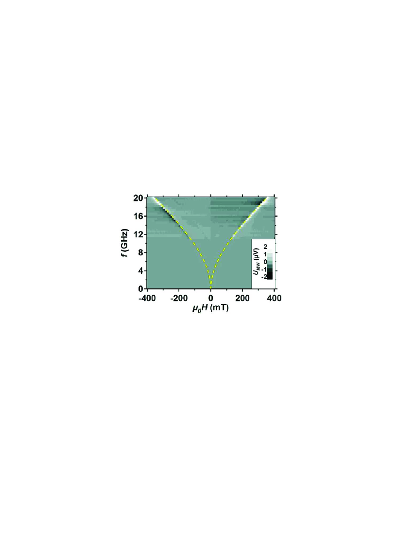
Figure 7: (Color online). Gray scale plot of the measured frequency and magnetic field dependence of the microwave photovoltage at $\alpha_{0}=47^{\circ}$. The dashed line shows the calculated FMR frequency (see equation (9)). The photovoltage intensity is strongly frequency dependent because of the frequency dependent waveguide transmission.

The exact position of the FMR is obscured by its strongly varying line shape. We overcome this problem by the productive line shape analysis in paragraph III.3. It is found that $H_{0}$ is slightly dependent on $\alpha_{0}$. This can be attributed to a small demagnetization field perpendicular to the stripes but within the film plane arising from the finite stripe dimensions in this direction. So, when $\mathbf{M_{0}}$ lies perpendicular to the stripe, $H_{0}$ slightly increases compared to the value fulfilling the Kittel equation for a plane (see equation (9)). In the parallel and perpendicular case we use the approximation of our film stripe as an ellipsoid, where we can use the corresponding Kittel equation Kittel (demagnetization factors $N_{x}$, $N_{y}$ and $N_{z}$ with respect to the dc magnetic field):

$$\omega=\gamma\sqrt{\left(H_{0}+\left(N_{x}-N_{z}\right)M_{0}\right)\left(H_{0}+\left(N_{y}-N_{z}\right)M_{0}\right)}$$ (50)

The difference of the resonance field between the case that $\mathbf{M}_{0}$ lies in the film plane parallel to the stripe and perpendicular is 1.6 mT (0.7%) at f = 15 GHz. From this we can calculate the small demagnetization factor $N_{x\prime}=0.085\%$ perpendicular to the Permalloy stripe within the film plane using equation (50). From the sum rule Iwata follows: $N_{y}=1-N_{x\prime}-N_{z\prime}=1-0.085\%-0=99.915\%$. $N_{z\prime}$ (parallel to the stripe) can be assumed to be negligibly small. This matches roughly with the dimension of the height to width ratio (49 nm : 200 $\mu$m) of the sample. For the stripe presented in section IV similar but stronger demagnetization effects are found.

Now we will have a closer look on the magnetic properties of the investigated film. Again at $f=15$ GHz we find using equation (10): $H_{0}=0.219$ T. Using asymmetric Lorentz line shape fitting as described in III.3 we get $\alpha_{G}=0.0072$. Consequently $A_{xx}=231.1$, $A_{xy}=97.1$ and $A_{yy}=40.8$ according to equation (13).

Because of $\alpha_{G}=0.0072$ the magnetization precession does impressive $n\approx 22$ turns before being damped to $1/e$ of its initial amplitude ($n=1/2\pi\alpha_{G}$). Therefore the ellipcity of $\mathbf{m}$ is almost independent of $\mathbf{h}$ (see paragraph II.2). It can be calculated from equation (35) that $m_{x}/m_{y}=2.38i$ at $\omega/2\pi$ = 15 GHz.

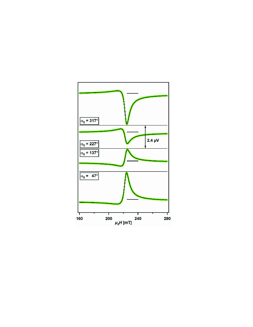
Figure 8: (Color online). Fitting (black line) of the microwave photovoltage signal (dots) for different angles $\alpha_{0}$ at $f=15$ GHz. The black horizontal bars indicate zero signal.

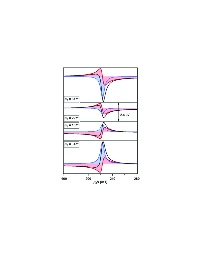
Figure 9: (Color online). Symmetric and Antisymmetric contributions to the asymmetric Lorentz line shape fit from figure 8 (black). A small constant background is found and added to the antisymmetric contribution.

To check the validity of our approximation ($d\ll\delta$, see II.2) we will now regard the skin depth $\delta$ at $f=15$ GHz in our sample ($d=49$ nm). For $\mu=\mu_{0}$ (away from the FMR) we find: $\delta=\sqrt{2/\omega\mu\rho}$ = 2.4 $\mu$m. Hence $\delta\gg d$. This is in accordance with our approximation that $\mathbf{h}$ is almost constant within the Permalloy film (see II.2). However in the vicinity of the FMR: $|\mu|\gg\mu_{0}$ and for the same frequency and conditions as above: $\mu_{L}=(1+\chi_{L})\mu_{0}=133i\mu_{0}$ at the FMR. Thus we approximate $\delta_{FMR}=\sqrt{2/\omega|\mu_{L}|\rho}=$ 210 nm. Hence $\delta_{FMR}$ is still significantly larger than $d$ and our approximation is still valid.

Finally we can summerize that for samples with weak damping ($\alpha_{G}\ll\omega/\omega_{M}$) like ours the approximation $H\approx H_{0}$ gives results with impressive precision (see figure 8) because its discrepancies are limited to the unimportant magnetic field ranges with $|\chi_{xx}|$, $|\chi_{xy}|$, $|\chi_{yy}|\ll 1$ which are far away from the FMR.

III.3 ASYMMETRIC LORENTZ LINE SHAPE

Although in section III.2 the frequency dependence of the FMR field is verified with the gray scale plot in figure 7, it is still desirable to receive a more accurate picture of the corresponding line shape which is found to be strongly angular dependent (see figure 8). In equation (46) it is shown that the magnetic field dependence of $U_{MW}$ exhibits asymmetric Lorentz line shape around $H=H_{0}$. Hence $U_{MW}$ takes the form

$$U_{MW}=U_{MW}^{SYM}+U_{MW}^{ANT}$$

$$=U_{0}^{SYM}\frac{\Delta H^{2}}{(H-H_{0})^{2}+\Delta H^{2}}$$ (51)

$$+U_{0}^{ANT}\frac{\Delta H(H-H_{0})}{(H-H_{0})^{2}+\Delta H^{2}}$$

This is used to fit the magnetic field dependence of the photovoltage in figure 8. For clearness the symmetric (absorptive) and antisymmetric (dispersive) contributions are shown separately in figure 9. A small constant background is found and added to the antisymmetric contribution. The background could possibly arise from other weak non-resonant photovoltage mechanisms.

The fits agree in an unambiguous manner with the measured results. Hence they can be used to determine the Gilbert damping parameter with high accuracy: $\alpha_{G}\approx\gamma\Delta H/\omega\approx(0.72\%\pm 0.015\%$). However if the magnetization lies parallel or perpendicular to the stripe the photovoltage vanishes (see equation (40)). Hence we can only verify $\alpha_{G}$ when the magnetization is neither close to being parallel nor perpendicular to our stripe.

The corresponding $\alpha_{G}=1/\omega\tau$ in the Nickel sample of Egan and JuretschkeEgan , can be estimated using the ferromagnetic relaxation time $\tau$ from their Table II. It lies in between $\alpha_{G}=0.12$ and 0.18, so being more than 16 times higher than the value in our sample. This makes the line shape approximation of section II.4 invalid for their case. Consequently a much more elaborated line shape analysisJuretschke appears necessary.

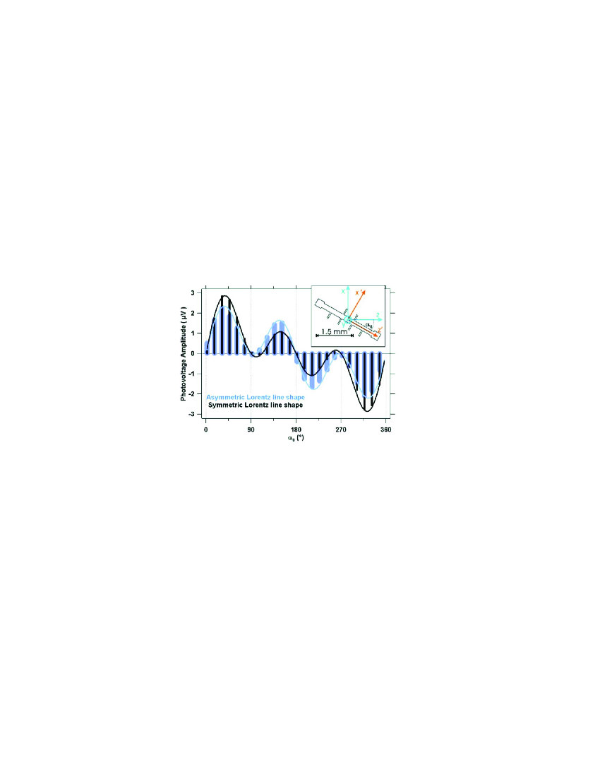
Figure 10: (Color online). The Bars show the angular dependence of the amplitude of the symmetric ($U_{0}^{SYM}$, thin bars) and antisymmetric ($U_{0}^{ANT}$, thick bars) contribution to the microwave photovoltage at f = 15.0 GHz. Note that both, the symmetric and antisymmetric contribution, vanish for $\alpha_{0}=0^{\circ},90^{\circ},180^{\circ}$ and $270^{\circ}$. The lines represent the corresponding fits by means of equation (53). The inlet shows the geometry of the investigated Permalloy stripe and the coordinate systems from figure 3 (note: $\mathbf{z}\parallel\mathbf{H}$).

In figure 8 the photovoltage along the stripe is presented at 4 different angles $\alpha_{0}$. The signal to noise ratio is about 1000 because of the carefully designed measurement system, where the noise is suppressed to less than 5 nV. Because of this good sensitivity we can verify the matching of our theory from section II with the measurement results in great detail.

In the following we want to investigate the angular dependence in detail. Therefore we transform the coordinate system of equation (II.4) according to the transformation presented in section II.1. Doing so we can separate the contributions from $h_{x\prime}$, $h_{y}$ and $h_{z\prime}$:

$$U_{MW}\ =\frac{R_{A}I_{1}\sin(2\alpha_{0})}{2M_{0}}\cdot$$

$$\{\left(A_{xy}h_{y}^{r}+A_{xx}(h_{x\prime}^{i}\cos\alpha_{0}-h_{z\prime}^{i}\sin\alpha_{0})\right)$$

$$\cdot\frac{\Delta H^{2}}{(H-H_{0})^{2}+\Delta H^{2}}$$ (52)

$$+\left(A_{xy}h_{y}^{i}+A_{xx}(h_{z\prime}^{r}\sin\alpha_{0}-h_{x\prime}^{r}\cos\alpha_{0})\right)$$

$$\cdot\frac{\Delta H(H-H_{0})}{(H-H_{0})^{2}+\Delta H^{2}}\}$$

$h_{x\prime}$, $h_{y}$ and $h_{z\prime}$ are fixed with respect to the hollow brass waveguide and its microwave configuration and do not change when $\alpha_{0}$ is varied.

We find that the angular dependence of the line shape in equation (III.3) exhibits 2 aspects: an overall factor $\sin(2\alpha_{0})$ and individual factors ($\sin\alpha_{0}$, $\cos\alpha_{0}$ and 1) for the terms belonging to the different spatial components of $\mathbf{h}$. The overall factor $\sin(2\alpha_{0})$ arises from the AMR photovoltage mechanism and results in vanishing of the photovoltage signal at $\alpha_{0}=0^{\circ},90^{\circ},180^{\circ}$ and $270^{\circ}$. This means if $\mathbf{M_{0}}$ lies either parallel, antiparallel or perpendicular to the stripe axis. This is illustrated in figure 11 and is clearly observed in our measurements (see figure 10). We take this as a strong support for the photovoltage being really AMR based.

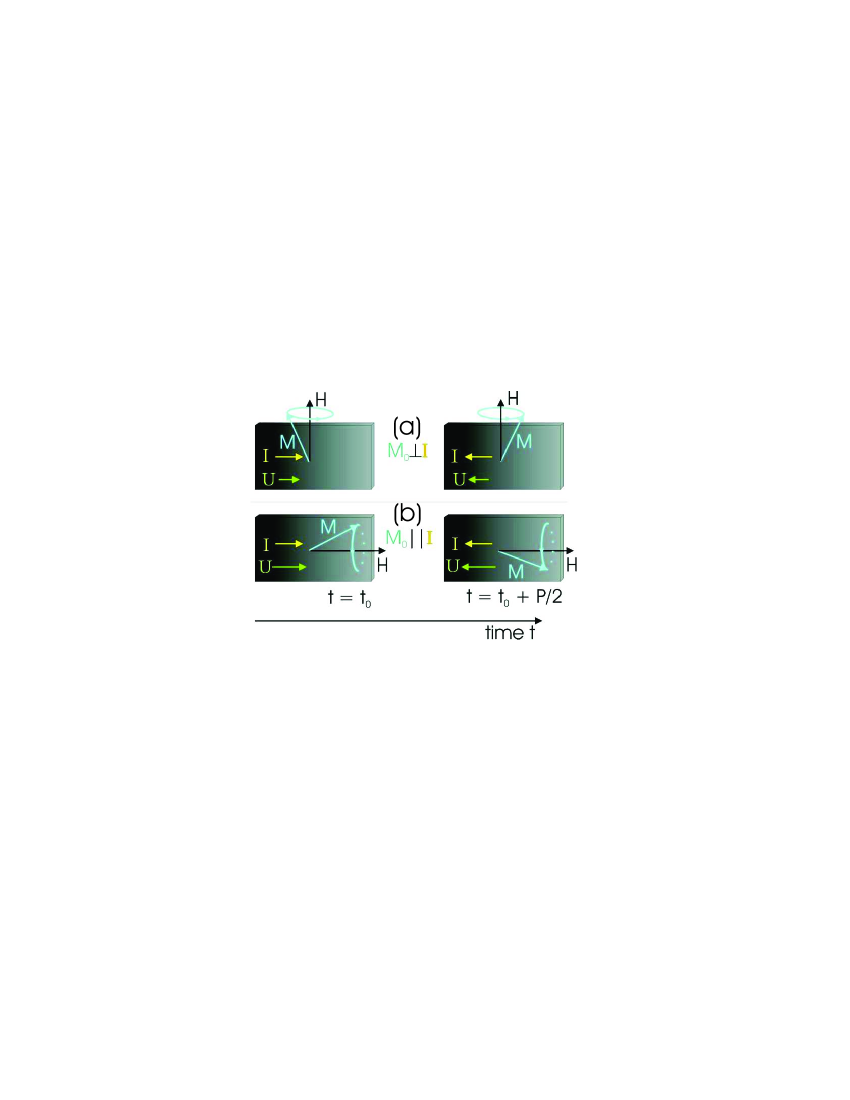
Figure 11: (Color online). When the magnetic field $\mathbf{H}$ lies parallel or perpendicular to the stripe, the time average voltage vanishes. (a) $\mathbf{H}$ lies perpendicular to $\mathbf{I}$: precession of the magnetization $\mathbf{M}$ leaves (after half a period P/2) the angle $\theta$ between the axis of $\mathbf{M}$ and $\mathbf{I}$ unchanged. Hence the AMR (and so voltage $\mathbf{U}$) is also unchanged. The photovoltage vanishes. (b) $\mathbf{H}$ is parallel to $\mathbf{I}$: $\theta$ and the AMR stay constant during the precession of $\mathbf{M}$ and the time average of $\mathbf{I}$ is zero. This means that only when $\mathbf{H}$ is neither parallel nor perpendicular to the stripe a photovoltage is generated.

Another support comes from the similarity with the planar Hall effect Yau . The planar Hall effect generates a voltage $U_{PHE}$ perpendicular to the current in ferromagnetic samples (width W) when the magnetization $\mathbf{M_{0}}$ lies in the current-voltage plane. It arises as well from AMR and vanishes when $\mathbf{M_{0}}$ lies either parallel or perpendicular to the current axis.

The similarity arises because of the AMR only generating a transversal resistance when the current is not lying along the principle axis of its resistance matrix (parallel or perpendicular to the magnetization). This is the same geometrical restriction as shown above for the microwave photovoltage (see equation (40) and figure 11).

We want to emphasize the importance that in any of these microwave photovoltage experiments, due to the unusually strong angle dependence, it is important to pay attention to the exact angle adjustment of the sample with respect to the dc magnetic field $\mathbf{H}$ when measuring under high symmetry conditions ($\mathbf{H}$ parallel or perpendicular to the stripe) to avoid involuntary signal changes due to small misalignments. As found in $90^{\circ}$ out-of-plane configuration GuiHu already a misalignment as small as a tenth of a degree can yield a tremendous photovoltage change in the vicinity of the FMR.

Finally we want to come back to the individual angular dependencies of the photovoltage contributions arising from the different external magnetic field components. In addition to the $\sin(2\alpha_{0})$ proportional dependence of $U_{MW}$ on $m_{x}$, also the strength with which $m_{x}$ is excited by $\mathbf{h}$ depends on $\alpha_{0}$. This is displayed in figure 12 and reflected by the three terms in equation (III.3) depending on $h_{x\prime}$, $h_{y}$ and $h_{z\prime}$ with $\cos\alpha_{0}$, 1 and $\sin\alpha_{0}$-factors respectively. Hence the symmetric $U_{0}^{SYM}$ and antisymmetric $U_{0}^{ANT}$ Lorentz line shape contribution to $U_{MW}$ are fitted in figure 10 with

$$U_{0}^{SYM}=(U_{z\prime}^{S}\sin(\alpha_{0})+U_{x\prime}^{S}\cos(\alpha_{0})+U_{y}^{S})\sin(2\alpha_{0})$$

$$U_{0}^{ANT}=(U_{z\prime}^{A}\sin(\alpha_{0})+U_{x\prime}^{A}\cos(\alpha_{0})+U_{y}^{A})\sin(2\alpha_{0})$$ (53)

From $U_{z\prime}^{S}$, $U_{x\prime}^{S}$ and $U_{y}^{A}$ the dynamic magnetic field components $h_{z\prime}^{i}$, $h_{x\prime}^{i}$, $h_{y}^{i}$ which are $90^{\circ}$ out-of-phase with respect to the rf current $I_{1}$ can be determined using equation (III.3) and from $U_{z\prime}^{A}$, $U_{x\prime}^{A}$ and $U_{y}^{S}$ we find $h_{z\prime}^{r}$, $h_{x\prime}^{r}$ and $h_{y}^{r}$ which are in phase with $I_{1}$.

In principle $I_{1}$ can be separately deduced using the bolometric effect Gui07c as discussed in section IV.1. However for the sample used here our usage of multiple stipes does not allow us to address the bolometric heating to one single stripe. Consequently the strength of $I_{1}$ is unknown so that we can not determine $\mathbf{h}$, but only $\mathbf{h}I_{1}$.

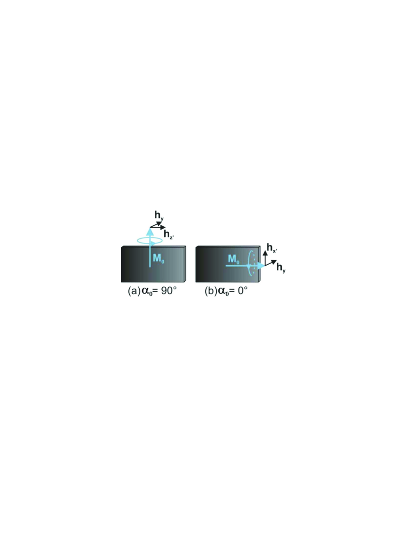
Figure 12: (Color online). Angular dependent coupling of the magnetization $\mathbf{M}$ to the dynamic magnetic field $\mathbf{h}=(h_{x\prime},h_{y},h_{z\prime})$. Only the components of $\mathbf{h}$ perpendicular to $\mathbf{M_{0}}$ can excite precession of $\mathbf{M}$ and therefore generate a dynamic $\mathbf{m}$. $h_{y}$ is always exciting $\mathbf{m}$. The excitation strength of $h_{x\prime}$ and $h_{z\prime}$ is angular dependent (compare equation (III.3)). Here the two symmetry cases are shown: $\mathbf{M}$ (a) perpendicular (only $h_{z\prime}$ and $h_{y}$ can excite $\mathbf{M}$) and (b) parallel (only $h_{x\prime}$ and $h_{y}$ can excite $\mathbf{M}$) to the stripe.

Besides, considering the special dynamic magnetic field configuration in our rectangular hollow waveguide no rf magnetic field component $h_{z\prime}$ is expected to be generated along the waveguides narrow dimension (z^′-axis) by the TE₀₁ mode Guru (which is the microwave configuration of our waveguide). It follows that the $\sin(\alpha_{0})$ terms in equation (53) vanishes. This results in the additional symmetry $U_{MW}(\alpha_{0})=-U_{MW}(-\alpha_{0})$, which is clearly observed in our measurements (see figure 10). This symmetry was broken when we used a round waveguide.

The vanishing of $h_{z\prime}$ in our waveguide will allow us to plot the direction of $\mathbf{h}$ 2 dimensional (instead of 3 dimensional) in figure 13. A small deviation from the symmetry $U_{MW}(\alpha_{0})=-U_{MW}(-\alpha_{0})$ is however found and arises from a small $h_{z\prime}$ component (see table 1) which is not displayed in figure 13. It might arise from the fact that the rf microwave magnetic field $\mathbf{h}$ at the waveguide end already deviates from the TE₀₁ mode.

III.4 DETERMINATION OF THE RF MAGNETIC FIELD DIRECTION

Using the different angular dependencies of the 3 symmetric and 3 antisymmetric terms in equation (III.3) $\mathbf{h}I_{1}$ can be determined. We make the assumption that the stripe itself does not influence the rf magnetic field configuration, what is at least the case when further reducing its dimensions. Thus the film stripe becomes a kind of detector for the rf magnetic field $\mathbf{h}$.

	$U^{S}_{x\prime,y,z\prime}$	$U^{A}_{x\prime,y,z\prime}$	$A_{xx}$	$A_{xy}$	$I_{1}\cdot h^{r}_{x\prime,y,z\prime}$	$I_{1}\cdot h^{i}_{x\prime,y,z\prime}$
	($\mu$V)				(mA$\cdot\mu$T$/\mu_{0})$
$x^{\prime}$	+2.60	+2.55	231.1		-15.7	+16.4
$y$	+0.95	+0.30		97.1	+14.0	+4.4
$z^{\prime}$	+0.12	0.00	231.1		0.0	-0.7

Table 1: Determination of the rf magnetic field $\mathbf{h}$ at the 200 $\mu$m wide stripe at 1 mm distance from the waveguide end by means of equation (III.3). $U^{S}_{x\prime,y,z\prime}$, $U^{A}_{x\prime,y,z\prime}$: Measured amplitudes of the contributions to the symmetric and antisymmetric Lorentz line shape of $U_{MW}$ (see equation (53)) with the angular dependence belonging to $x^{\prime}$, $y$ and $z^{\prime}$ respectively (taken from the fitting in figure 10). $A_{xx,xy}$: Corresponding amplitudes of $\chi_{xx,xy}$. $h^{r}_{x\prime,y,z\prime}$, $h^{i}_{x\prime,y,z\prime}$: rf magnetic field strength calculated from $U^{S}_{x\prime,y,z\prime}$, $U^{A}_{x\prime,y,z\prime}$ (in-phase and 90^∘ out-of-phase contribution with respect to the current).

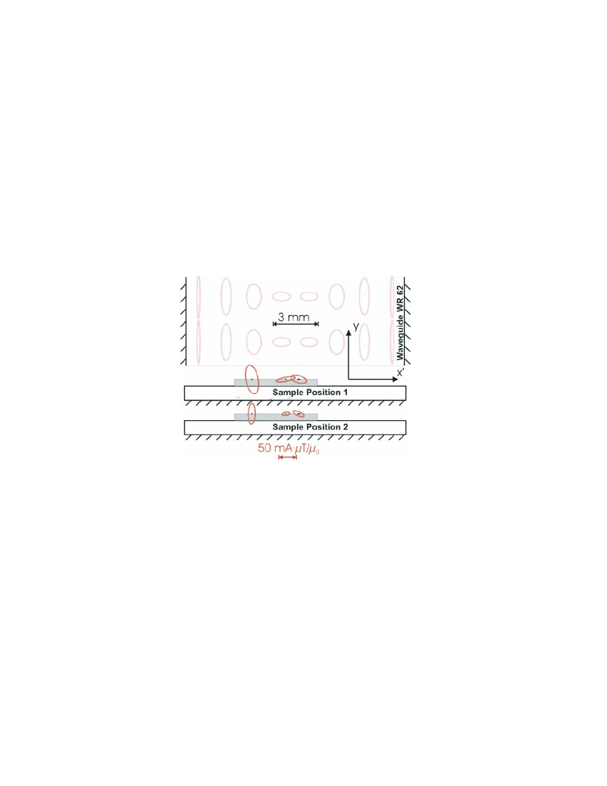
Figure 13: (Color online). Direction and ellipticity of the rf magnetic field $\mathbf{h}$ displayed by showing the path $I_{1}\cdot\mathbf{h}$ passes during one cycle. This is shown at the location of the 3 stripes (these lie normal to the picture on top of the gray GaAs-substrate; the 200 $\mu$m wide stripe to the right) for two sample positions. $I_{1}\cdot\mathbf{h}$ was determined by means of equation (III.3). The upper right path corresponds to the $I_{1}\cdot\mathbf{h}$ from table 1. The hatched edges indicate metal surfaces reflecting microwaves. Within the waveguide the rf magnetic field $\mathbf{h}$ corresponding to the TE₁₀-mode is displayed in the background.

To test this an array of 36 additional 50 $\mu$m wide and 20 $\mu$m distant Permalloy stripes of the same height and length as the 200 $\mu$m wide stripe described above (see section III.1) was patterned beside this one. The 50 $\mu$m wide stripes were connected with each other at alternating ends to form a long meandering stripeGui . Four stripes were elongated on both ends to 300$\times$300 $\mu$m² Permalloy contact pads. For the outer two stripes and the single 200 $\mu$m stripe $\mathbf{h}I_{1}$ is calculated from the measured photovoltage using equation (II.4). Table 1 shows the measured voltage and the corresponding $\mathbf{h}I_{1}$ for the 200 $\mu$m stripe at 1 mm distance from the waveguide. $\mathbf{h}I_{1}$ for all 3 stripes is displayed in figure 13, while positioning the sample at 2 distances (1 and 3.5 mm respectively) from the waveguide end. For comparison the rf magnetic field $\mathbf{h}$ configuration of the TE₀₁-mode is displayed in the background. From other measurements we can estimate that $I_{1}$ lies somewhere in the 1 mA-range.

It is worth noting that possible inhomogeneities of the rf magnetic field $\mathbf{h}$ within the Permalloy stripes will be averaged because $U_{MW}$ is linear in $\mathbf{h}$. Determining the sign of the rf magnetic field components from the photovoltage contributions signs exhibits a certain complexity because a lot of attention has to be paid to the chosen time evolution ($e^{i\omega t}$ or $e^{-i\omega t}$) and coordinate system (right hand or left hand). However the sign only reflects the phase difference with respect to the rf current. The rf current is admittedly not identical for different stripe positions. Consequently the comparison of the rf magnetization phase at different stripe locations is obscured.

It is a specially interesting point concerning microwave photovoltage that the phase of the individual components of the rf magnetic field with respect to the rf current, and therefore also with respect to each other can be determined. The phase information is encoded in the line shape, which is a particular feature of the microwave photovoltage described in this work.

At this point only determining $\mathbf{h}I_{1}$ is possible because $I_{1}$ is unknown. However in paragraph IV.1 an approach to determine $I_{1}$ using the bolometric effect is presented. Using this approach the bolometric photoresistance is the perfect supplement for the photovoltage. It delivers unknown $I_{1}$ with almost no additional setup.

IV PHOTORESISTANCE MEASUREMENTS

The principle difficulties when detecting the AMR induced photoresistance are to increase the microwave power for a sufficient signal strength and to reduce the photovoltage signal, which is in general much stronger and superimposes with the photoresistance. We overcome the microwave power problem by using high initial microwave power (316 mW) and a coplanar waveguide (CPW) GuiHu which emits the microwaves as close as possible to the Permalloy film stripe ($0.137\times 20\times 2450\ \mu$m³) with which we detect the photoresistance. Its resistance is found to be $R=880\ \Omega$ and the AMR $R_{A}=15\ \Omega$. Its magnetic properties ($\gamma$, $M_{0}$) are almost identical to that of the sample investigated in section III. We use again lock-in technique like in III.1 with now an additional dc current from a battery to measure resistance instead of voltage. The strong microwave power results in strong rf currents within the sample which give a specially strong photovoltage signal (see equation (46)). To achieve a sufficiently strong photoresitance signal the dc current $I_{0}$ and rf current $I_{1}$ have to be increased to the maximal value that does not harm the sample (a few mA, hence $I_{0}\approx I_{1}$).

Ignoring the trigonometric factors $\sin 2\alpha_{0}$, $\cos 2\alpha_{0}$ and $\cos\psi$ as well as the photoresistance term depending on $\beta_{1}$ (that is always smaller than $\alpha_{1}$) the photovoltage signal ($U_{MW}=\alpha_{1}\sin(2\alpha_{0})\cos\psi R_{A}I_{1}/2$, equation (40)) and the photoresistance signal ($\Delta R_{MW}I_{0}\approx-\alpha_{1}^{2}\cos(2\alpha_{0})R_{A}I_{0}/2$, (36)) become almost identical. But the major difference is that the photoresistance is multiplied by $\alpha_{1}^{2}$ and the photovoltage only by $\alpha_{1}$. As $\alpha_{1}$ is particularly small ($<1^{\circ}$) in our experiments, this means that $\Delta R_{MW}I_{0}$ is much smaller than $U_{MW}$. However suppressing $U_{MW}$ is possible because it vanishes for $\alpha_{0}=0^{\circ},\ 90^{\circ},\ 180^{\circ},\ 270^{\circ}$ (see equation (40)). A very precise tuning of $\alpha_{0}$ with an accuracy below $0.1^{\circ}$ is necessary to suppress $U_{MW}$ below $\Delta R_{MW}I_{0}$. Fortunately in contrast to $|U_{MW}|$, $|\Delta R_{MW}|$ is maximal for $\alpha_{0}=0^{\circ},\ 90^{\circ},\ 180^{\circ},\ 270^{\circ}$. In the following we will first discuss the bolometric photoresistance arising from microwave heating of the sample and afterwards the AMR induced photoresistance that is discussed above.

IV.1 BOLOMETRIC (NON-RESONANT)

The AMR-induced $\Delta R_{MW}$ is not the only photoresistive effect present in our Permalloy film stripe. Also non-resonant heating by the microwave rf current $I_{1}$ results in a (bolometric) photoresistance. The major difference compared to the AMR-based photoresistance is that the bolometric photoresistance is almost independent of the applied dc magnetic field $H$ and that its reaction time to microwave exposure is much longer (in the order of ms) than that of the AMR-based photresistance ($1/\alpha_{G}\omega$, in the order of ns) Gui07c . The non-resonant bolometric photoresistance is found with a typical strength of $(\Delta R/R)/P=$ 0.2 ppm/mW (see figure 14).

The bolometric heating power $P_{bol}$ arises from resistive dissipation of the rf current $I_{1}$ in the sample ($P_{bol}=\left<RI^{2}\right>=RI_{0}^{2}+RI_{1}^{2}/2$). This can hence be used to determine $I_{1}$, which is otherwise an unknown in equation (46). $I_{1}$ can be determined for example by finding the corresponding dc current $I_{0}$ with the same bolometric resistance change. However, especially in the sample we use the thermal conductivity of the GaAs-crystal on which our Permalloy stripes were deposited is so high (55 W$/$m$\cdot$K) that the different stripes are strongly thermally coupled. Thus we can not address the bolometric signal of one stripe solely to the rf current of the same stripe. This effect was verified comparing the resistance changes from one stripe while applying a dc current through an other stripe. Hence determination of $|I_{1}|$ by means of equation (46) is only possible when using a substrate material with low heat conductance (e.g. glass) or by not depositing more than one stripe.

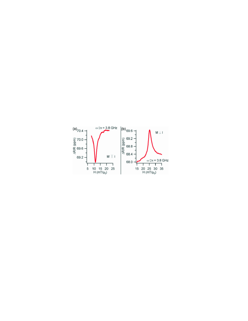
Figure 14: (Color online). Photoresistance $\Delta R_{MW}$ measurement (stripe resistance $R$). The curves show the difference between the signals $\Delta U$ with $I_{0}=+5$ mA and $I_{0}=-5$ mA at $P=316$ mW: $\Delta R=(\Delta U(I_{0}=+5$ mA$)-\Delta U(I_{0}=-5$mA$))/10$ mA. The subtraction suppresses the photovoltage dependence on absolute $|I_{0}|$ (for example from bolometric AMR change). For both curves the dc magnetic field $\mathbf{H}$ (and so $\mathbf{M}$) was applied within the film plane, but for a) parallel to the stripe (and hence to the dc current $I_{0}$) and for b) perpendicular. A non-resonant background of about 70 ppm from bolometric photoresistance is found. It is decreases by about 1.2 ppm when the sample is turned from parallel to perpendicular configuration. This is caused by the 1.7 % AMR which changes $R$ and the bolometric signal proportionally. The FMR signal has almost Lorentz line shape and its position is significantly changing when the sample is turned from parallel to perpendicular position (see section IV.2).

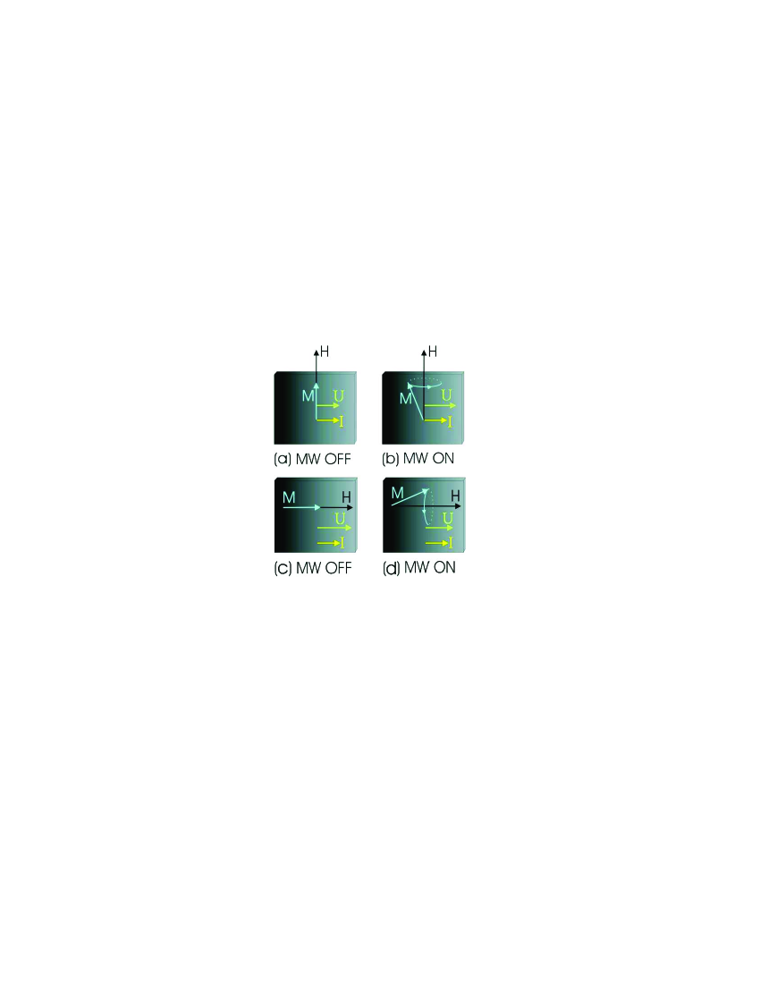
Figure 15: (Color online). Demonstration of the angular dependence of the microwave photovoltage: Without microwaves (a,c) the AMR is minimal in perpendicular configuration (a) of $\mathbf{M}$ and $\mathbf{I}$ and maximal in parallel configuration (c). When the microwaves are switched on the resistance increases in parallel configuration (b) and decreases in perpendicular configuration (d).

IV.2 AMR BASED (RESONANT)

In contrast to the non-resonant bolometric photoresistance in IV.1, the typically 50 times weaker resonant AMR-based photoresistance is very hard to detect. After visualizing it by using the CPW and turning the sample into a high symmetry position (parallel or perpendicular to $\mathbf{H}$) it is still necessary to regard the difference of the photoresistance measured with the same current strength but with reversed current sign instead of measuring with only one current direction. This eliminates the remaining still significant photovoltage signal, which depends on the absolute current strength possibly due to bolometric AMR change.

Measurement results are presented in figure 14 for $f=3.8$ GHz. There it can be seen that (as deduced in II.3), if the stripe lies parallel to the magnetization, the AMR is maximal and the resistance decreases when the FMR is excited (negative photoresistance). In contrast in the perpendicular case the AMR is minimal and we measure a resistance increase (positive photoresistance). This behavior is schematically explained in figure 15. The curves in figure 14 show the photoresistance at the FMR with symmetric Lorentz line shape as predicted in II.3.

Using equation (9) we calculate $\mu_{0}H_{0}=16.6$ mT. However a deviation of $H_{0}$ is found in both, parallel ($\mu_{0}H_{0}=11.1$ mT) and perpendicular ($\mu_{0}H_{0}=25.3$ mT), configuration. This is due to demagnetization which gives rise to an FMR shift with respect to the result from the infinite film approximation (compare equation (50)). $N_{x}=0.7\%$ can be assumed because of this shift.

Using equation (35) we find that for our conditions $m_{x}/m_{y}=7.9i$. Consequently we can neglect the contribution from $\beta_{1}=|m_{y}|/M_{0}$ in equation (36) and find $|m_{x}|=13$ mT using $\Delta R_{MW}=(\Delta R/R)\cdot R=1.23$ m$\Omega$ (from figure 14) and thus $\alpha_{1}=\sqrt{2\cdot\Delta R_{MW}/R_{A}}=0.73^{\circ}$ and $\beta_{1}=\alpha_{1}/|m_{x}/m_{y}|=0.09^{\circ}$. The smallness of $\beta_{1}$ is the reason for the resonant photoresistance strength being almost identical for $\mathbf{M}\parallel\mathbf{I}$ and $\mathbf{M}\perp\mathbf{I}$ (although the sign is reversed). We must expect $|m_{x}|$, $\alpha_{1}$ and $\beta_{1}$ to be even a little bit larger due to our lock-in measurement technique only detecting the sinusoidal contribution to the square wave signal from the microwaves.

The photoresistive decrease is in accordance with that found by Costache et al. Costache06 . There the magnetization is aligned with the current ($\alpha_{0}=0$). Thus applying an rf magnetic field decreases the AMR from $R_{A}$ to $R_{A}\cos^{2}\theta_{c}$. This is used to determine the precession cone angle $\theta_{c}$ by assuming $\theta_{c}=\alpha_{1}=\beta_{1}$.

The height to width ratio of the strip is 35 nm to 300 nm. Because of the magnetization lying along the stripe,Costache06 the magnetization precession strongly deviates from being circular. Using the corresponding parameters $\mu_{0}M_{0}=1.06$ T, $\gamma=2\pi\mu_{0}\cdot 28$ GHz/T and $\omega/2\pi=10.5$ GHz), we find from equation (35) that the ratio of the amplitudes is $m_{x}/m_{y}=3.15i$. This indicates strongly elliptical precession and suggests that distinguishing $\alpha_{1}$ and $\beta_{1}$ would provide a refined description compared to that using the cone angle $\theta_{c}$, as discussed in paragraph II.3.

V CONCLUSIONS

We have presented a comprehensive study of dc electric effects induced by ferromagnetic resonance in Py microstrips. A theoretical model based on a phenomenological approach to magnetoresistance is developed and compared with experiments. These provide a consistent description of both photovoltage and photoresistance effects.

We demonstrate that the microwave photoresistance is proportional to the square of magnetization precession amplitude. In the special case of circular magnetization precession, the photoresistance measures its cone angle. In the general case of arbitrary sample geometry and elliptical precession, we refine the cone angle concept by defining 2 different angles, which provide a precise description of the microwave photoresistance (and photovoltage) induced by elliptical magnetization precession. We show that the microwave photoresistance can be either positive or negative, depending on the direction of the dc magnetic field.

In contrast to the microwave photoresistance, we find that the microwave photovoltage is proportional to the product of the in-plane magnetization precession component with the rf current. Consequently it is sensitive to the magnetic field dependent phase difference between the rf current and the rf magnetization. This results in a characteristic asymmetric photovoltage line shape, which crosses zero when the rf current and the in-plane component of the rf magnetization are exactly 90^∘ out of phase. Therefore, the microwave photovoltage provides a powerful insight into the phase of magnetization precession, which is usually difficult to obtain.

We demonstrate that the asymmetric photovoltage line shape is strongly dependent on the dc magnetic field direction, which can be explained by the directional dependence of the magnetization precession excitation. By using the model developed in this work, and by combining such a sensitive geometrical dependence of the microwave photovoltage with the bolometric photoresistance which independently measures the rf current, we are now in a position to detect and determine the external rf magnetic field vector, which is of long standing interest with significant potential applications.

References

- (1) B. S. Guru and H. R. Hiziroglu, Electromagnetic Field Theory Fundamentals, Second Edition (Cambridge University Press, 2004).
- (2) B. A. Gurney et al., J. Shi, and R. R. Katti, in Ultrathin Magnetic Structures IV edited by B. Heinrich and J.A.C. Bland (Springer, Berlin, 2004), Chapter 6,7 and 8.
- (3) J.-G. Zhu, and Y. Zheng, in Spin Dynamics in Confined Magnetic Structures I edited by B. Hillebrands and K. Ounadjela (Spinger, Berlin, 2002), P. 289-323.
- (4) A. A. Tulapurkar et al., Nature , 339 (2005)
- (5) J. C. Sankey et al., Phys. Rev. Lett. , 227601 (2006).
- (6) A. Azevedo, L. H. Vilela Le o, R. L. Rodriguez-Suarez, A. B. Oliveira, and S. M. Rezende, J. Appl. Phys. 97, 10C715 (2005).
- (7) E. Saitoh, M. Ueda, H. Miyajima, and G. Tatara, Appl. Phys. Lett. 88, 182509 (2006).
- (8) M.V. Costache, M. Sladkov, S. M. Watts, C. H. van der Wal, and B. J. van Wees, Phys. Rev. Lett. 97, 216603 (2006); J. Grollier, M. V. Costache, C. H. van der Wal, and B. J. van Wees, J. Appl. Phys. 100, 024316 (2006).
- (9) Y. S. Gui, S. Holland, N. Mecking, and C.-M. Hu, Phys. Rev. Lett. , 056807 (2005).
- (10) Y. S. Gui, N. Mecking, X. Zhou, Gwyn Williams, and C.-M. Hu, Phys. Rev. Lett. 107602 (2007).
- (11) Y. S. Gui, N. Mecking, and C.-M. Hu, Phys. Rev. Lett. , 217603 (2007).
- (12) Y. S. Gui, N. Mecking, A. Wirthmann, L. H. Bai, and C.-M. Hu, Appl. Phys. Lett. , 082503 (2007).
- (13) M.V. Costache, S. M. Watts, M. Sladkov, C. H. van der Wal, and B. J. van Wees, Appl. Phys. Lett. 89, 232115 (2006)
- (14) A. Yamaguchi, H. Miyajima, T.Ono, Y. Suzuki, S. Yuasa, A. Tulapurkar, and Y. Nakatani, Appl. Phys. Lett. , 182507 (2007); ibid, , 212505 (2007).
- (15) Dong Keun Oh, et al. J. Magn. Magn. Mater. 293, 880 (2005); Je-Hyoung Lee and Kungwon Rhie, IEEE Trans. on Mag. 35, 3784 (1999).
- (16) S. T. Goennenwein, S. W. Schink, A. Brandlmaier, A. Boger, M. Opel, R. Gross, R. S. Keizer, T. M. Klapwijk, A. Gupta, H. Huebl, C. Bihler, and M. S. Brandt, Appl. Phys. Lett. , 162507 (2007).
- (17) J.C. Slonczewski, J. Magn. Magn. Mater. 159, L1 (1996).
- (18) L. Berger, Phys. Rev. B 54, 9353 (1996).
- (19) L. Berger, Phys. Rev. B 59, 11465 (1999).
- (20) A. Brataas, Yaroslav Tserkovnyak, Gerrit E. W. Bauer, and Bertrand I. Halperin, Phys. Rev. B 66, 060404(R) (2002).
- (21) Xuhui Wang, Gerrit E. W. Bauer, Bart J. van Wees, Arne Brataas, and Yaroslav Tserkovnyak, Phys. Rev. Lett. 97, 216602 (2006).
- (22) C.-M. Hu, C. Zehnder, Ch. Heyn, and D. Heitmann, Phys. Rev. B 67, 201302(R) (2003).
- (23) H. J. Juretschke, J. Appl. Phys. , 1401 (1960).
- (24) R.H. Silsbee, A. Janossy, and P. Monod, Phys. Rev. B 19, 4382 (1979).
- (25) W. M. Moller, and H. J. Juretschke, Phys. Rev. B , 2651 (1970).
- (26) D. Polder, Philosophical Magazine , 99 (1949).
- (27) T. L. Gilbert, IEEE Trans. on Magn. , 3443 (2004).
- (28) L. Landau, and L. Liftshitz, Physik Z. Sowjet. 153 (1935).
- (29) R. E. Camley, and D. L. Mills, J. Appl. Phys. , 3058 (1997).
- (30) C. Kittel, Phys. Rev. , 155 (1948).
- (31) W. G. Egan, and H. J. Juretschke, J. Appl. Phys. , 1477 (1963).
- (32) J. N. Kupferschmidt, Shaffique Adam, and P. W. Brouwer, Phys. Rev. B , 134416 (2006).
- (33) S. I. Kiselev, J. C. Sankey, I. N. Krivorotov, N. C. Emley, R. J. Schoelkopf, R. A. Buhrman, and D. C. Ralph, Nature , 380 (2003).
- (34) M. S. Sodha and N. C. Srivasta Microwave Propagation in Ferrimagnets (Plenum Press, New York, 1981).
- (35) K. L. Yau, and J. T. H. Chang, J. Phys. F , 38 (1971).