Sestieri of Venice

Abstract

We have investigated space syntax of Venice by means of random walks. Random walks being defined on an undirected graph establish the Euclidean space in which distances and angles between nodes acquire the clear statistical interpretation. The properties of nodes with respect to random walks allow partitioning the city canal network into disjoint divisions which may be identified with the traditional divisions of the city (sestieri).

PACS: 89.65.Lm, 89.75.Fb, 05.40.Fb, 02.10.Ox

Keywords: Complex networks, city space syntax

1 The Sestieri of Venice

Spectral methods can be implemented in order to visualize graphs of not very large multi-component networks [1]. City districts constructed accordingly to different development principles in different historical epochs can be envisioned on the dual graph representation of space syntax.

We investigate the segmentation of the spatial network of 96 canals in Venice (that stretches across 122 small islands between which the canals serve the function of roads) in accordance to its historical divisions.

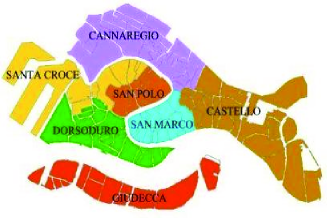
Figure 1: The sestieri are the primary traditional divisions of Venice. The image has been taken from ’Portale di Venezia’ at http://www.guestinvenice.com/

The sestieri are the primary traditional divisions of Venice (see Fig. 1): Cannaregio, San Polo, Dorsoduro, Santa Croce, San Marco and Castello, Giudecca. The oldest settlements in Venice had appeared from the 6^th century in Dorsoduro, along the Giudecca Canal. By the 11^thcentury, settlement had spread across to the Grand Canal. The Giudecca island is composed of 8 islets separated by canals dredged in the 9^th century when the area was divided among the rebelling nobles. San Polo is the smallest of the six sestieri of Venice, covering just 35 hectares along the Grand Canal. It is one of the oldest parts of the city, having been settled before the 9^th century, when it and San Marco (lying in the heart of the city) formed part of the Realtine Islands. Cannaregio named after the Cannaregio Canal is the second largest district of the city. It was developed from the 11^th century. Santa Croce occupies the north west part of the main islands lying on land only created form the late Middle ages to the twentieth century. The district Castello grew up from the 13^th century.

In the present paper, we address the following question: Given a spatial network of a city, is it possible to uncover its historical and functional divisions directly from its space syntax?

In Sec. 2, we discuss the primary and dual graph representations of urban environments. The dual graph representation has been extensively studied in space syntax theory which is instrumental in predicting human behavior in urban environments. In Sec. 3, we demonstrate that space syntax is related to the traffic equilibrium state of a transport network, and Markov’s transition operators naturally appear in the space syntax context embedding city space syntax into Euclidean space. We build the dual graph representation of Venetian canals in Sec. 4, 5 and then perform the Principal Component Analysis of Venetian space syntax in Sec 6. The properties of nodes with respect to random walks allow partitioning the city canal network into disjoint divisions which may be identified with the traditional divisions of the city (sestieri).

2 Graphs and Space Syntax of Urban Environments

Urban space is of rather large scale to be seen from a single viewpoint; maps provide us with its representations by means of abstract symbols facilitating our perceiving and understanding of a city. The middle scale and small scale maps are usually based on Euclidean geometry providing spatial objects with precise coordinates along their edges and outlines.

There is a long tradition of research articulating urban environment form using graph-theoretic principles originating from the paper of Leonard Euler (see [2]). Graphs have long been regarded as the basic structures for representing forms where topological relations are firmly embedded within Euclidean space. The widespread use of graph theoretic analysis in geographic science had been reviewed in [3] establishing it as central to spatial analysis of urban environments. In [4], the basic graph theory methods had been applied to the measurements of transportation networks.

Network analysis has long been a basic function of geographic information systems (GIS) for a variety of applications, in which computational modelling of an urban network is based on a graph view in which the intersections of linear features are regarded as nodes, and connections between pairs of nodes are represented as edges [5]. Similarly, urban forms are usually represented as the patterns of identifiable urban elements such as locations or areas (forming nodes in a graph) whose relationships to one another are often associated with linear transport routes such as streets within cities [6]. Such planar graph representations define locations or points in Euclidean plane as nodes or vertices $\{i\}$, $i=1,\ldots,N$, and the edges linking them together as $i\sim j$, in which $\{i,j\}=1,2,\ldots,N.$ The value of a link can either be binary, with the value $1$ as $i\sim j$, and $0$ otherwise, or be equal to actual physical distance between nodes, $\mathrm{dist}(i,j)$, or to some weight $w_{ij}>0$ quantifying a certain characteristic property of the link. We shall call a planar graph representing the Euclidean space embedding of an urban network as its primary graph. Once a spatial system has been identified and represented by a graph in this way, it can be subjected to the graph theoretic analysis.

A spatial network of a city is a network of the spatial elements of urban environments. They are derived from maps of open spaces (streets, places, and roundabouts). Open spaces may be broken down into components; most simply, these might be street segments, which can be linked into a network via their intersections and analyzed as a networks of movement choices. The study of spatial configuration is instrumental in predicting human behavior, for instance, pedestrian movements in urban environments [8]. A set of theories and techniques for the analysis of spatial configurations is called space syntax [9]. Space syntax is established on a quite sophisticated speculation that the evolution of built form can be explained in analogy to the way biological forms unravel [7]. It has been developed as a method for analyzing space in an urban environment capturing its quality as being comprehendible and easily navigable [8]. Although, in its initial form, space syntax was focused mainly on patterns of pedestrian movement in cities, later the various space syntax measures of urban configuration had been found to be correlated with the different aspects of social life, [10].

Decomposition of a space map into a complete set of intersecting axial lines, the fewest and longest lines of sight that pass through every open space comprising any system, produces an axial map or an overlapping convex map respectively. Axial lines and convex spaces may be treated as the spatial elements (nodes of a morphological graph), while either the junctions of axial lines or the overlaps of convex spaces may be considered as the edges linking spatial elements into a single graph unveiling the topological relationships between all open elements of the urban space. In what follows, we shall call this morphological representation of urban network as a dual graph.

The transition to a dual graph is a topologically non-trivial transformation of a planar primary graph into a non-planar one which encapsulates the hierarchy and structure of the urban area and also corresponds to perception of space that people experience when travelling along routes through the environment.

In Fig. 1, we have presented the glossary establishing a correspondence between several typical elements of urban environments and the certain subgraphs of dual graphs. The dual transformation replaces the 1D open segments (streets) by the zero-dimensional nodes, Fig. 1(1).

1.		2.
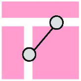
3.		4.
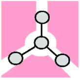
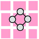
5.		6.

Figure 2: The dual transformation glossary between the typical elements of urban environments and the certain subgraphs of dual graphs.

The sprawl like developments consisting of a number of blind passes branching off a main route are changed to the star subgraphs having a hub and a number of client nodes, Fig. 1(2). Junctions and crossroads are replaced with edges connecting the corresponding nodes of the dual graph, Fig.1(3). Places and roundabouts are considered as the independent topological objects and acquire the individual IDs being nodes in the dual graph Fig. 1(4). Cycles are converted into cycles of the same lengthes Fig. 1(5). A regular grid pattern is shown in Fig. 1(6). Its dual graph representation is called a complete bipartite graph, where the set of vertices can be divided into two disjoint subsets such that no edge has both end-points in the same subset, and every line joining the two subsets is present, [11]. These sets can be naturally interpreted as those of the vertical and horizontal edges in the primary graphs (streets and avenues). In bipartite graphs, all closed paths are of even length, [12].

It is the dual graph transformation which allows to separate the effects of order and of structure while analyzing a transport network on the morphological ground. It converts the repeating geometrical elements expressing the order in the urban developments into the twins nodes, the pairs of nodes such that any other is adjacent either to them both or to neither of them. Examples of twins nodes can be found in Fig. 1(2,4,5,6).

3 Traffic Equilibrium, Space Syntax, and Random Walks

The concept of equilibrium, the condition of a system in which all competing influences are balanced, is a key theoretical element in any branch of science. The notion of traffic equilibrium had been introduced by J.G. Wardrop [13] and then generalized by [14] to a fundamental concept of network equilibrium with many potential applications such as the establishing of rigorous mathematical foundations for the analysis of congested transport networks. Wardrop’s traffic equilibrium [13] is strongly tied to city space syntax since it is required that while attaining the equilibrium all travellers have enough knowledge of the transport network they use. Because of the complexity of traffic situation in the network, the route choice decisions taken by travellers are not always objectively optimal. However, there is another link between the traffic equilibrium and space syntax which has never been discussed in the literature.

Given a connected undirected graph $G(V,E)$, in which $V$ is the set of nodes and $E$ is the set of edges, we can define the traffic volume $f:E\to(0,\infty[$ through every edge $e\in E$. It then follows from the Perron-Frobenius theorem that a linear equation

$$f(e)\,=\,\sum_{e^{\prime}\,\in\,E}\,f(e^{\prime})\,\exp\left(\,-h\,\ell\left(e^{\prime}\right)\,\right)$$ (1)

has a unique positive solution $f(e)>0$, for every edge $e\in E$, for a fixed positive constant $h>0$ and a chosen set of positive metric length distances $\ell(e)>0$. This solution is naturally identified with the traffic equilibrium state of the transport network defined on $G$, in which the permeability of edges depends upon their lengths. The parameter $h$ is called the volume entropy of the graph $G$, while the volume of $G$ is defined as the sum

$$\mathrm{Vol}(G)=\frac{1}{2}\sum_{e\in E}\ell(e).$$ (2)

The degree of a node $v\in V$ is the number of its neighbors in $G$, $\deg(v)=k_{v}$. It has been shown in [15] that among all undirected connected graphs of normalized volume, $\mathrm{Vol}(G)=1$, which are not cycles and $k_{v}\neq 1$ for all nodes, the minimal possible value of the volume entropy,

$$\min(h)=\frac{1}{2}\sum_{v\in V}k_{v}\,\log\left(k_{v}-1\right)$$ (3)

is attained for the length distances

$$\ell(e)\,=\,\frac{\log\left(\left(k_{i(e)}-1\right)\left(k_{t(e)}-1\right)\right)}{2\,\min(h)},$$ (4)

where $i(e)\in V$ and $t(e)\in V$ are the initial and terminal vertices of the edge $e\in E$ respectively. It is then obvious that (4) and $\min(h)$ being substituted into (1) change the operator $\exp\left(-h\ell(e)\right)$ to a symmetric Markov transition operator,

$$f(e)\,=\,\sum_{e^{\prime}\,\in\,E}\,\frac{f(e^{\prime})}{\sqrt{\left(k_{i(e)}-1\right)\left(k_{t(e)}-1\right)}},$$ (5)

which rather describes time reversible random walks over edges than over nodes. The flows satisfying (1) with the Markov operator (5) meet the mass conservation property,

$$\sum_{i\sim j}f_{ij}=\pi_{j},\quad\sum_{j\in V}\pi_{j}=1,$$ (6)

for some node constants $\pi_{i}>0$. Other solutions $f(e)>0$ obtained for $h\,>\min(h)$ describe equilibrium flows with termination of travellers. The Eq.(5) unveils the indispensable role Markov’s chains defined on edges play in equilibrium traffic modelling and exposes the degrees of nodes as a key determinant of the transport networks properties.

Random walks embed connected undirected graphs into Euclidean space, in which distances and angles acquire the clear statistical interpretation.

Any graph representation naturally arises as an outcome of categorization, when we abstract a real world system by eliminating all but one of its features and by the grouping of things (or places) sharing a common attribute by classes or categories. For instance, the common attribute of all open spaces in city space syntax is that we can move through them. All elements called nodes that fall into one and the same group $V$ are considered essentially identical; permutations of them within the group are of no consequence. The symmetric group $\mathbb{S}_{N}$ consisting of all permutations of $N$ elements ($N$ is the cardinality of the set $V$) constitute the symmetry group of $V$. If we denote by $E\subseteq V\times V$ the set of ordered pairs of nodes called edges, then a graph is a map $G(V,E):E\to K\subseteq\mathbb{R}_{\,+}$ (we suppose that the graph has no multiple edges).

The nodes of $G(V,E)$ may be weighted with respect to some measure $m=\sum_{i\in V}m_{i}\delta_{i},$ specified by a set of positive numbers $m_{i}>0$. The space $\ell^{2}(m)$ of square-assumable functions with respect to the measure $m$ is the Hilbert space $\mathcal{H}$ (a complete inner product space). Among all linear operators defined on $\mathcal{H}$, those invariant under the permutations of nodes are of essential interest since they reflect the symmetry of the graph. Although there are infinitely many such operators, only those which maintain conservation of a quantity may describe a physical process. The Markov transition operators which share the property of probability conservation considered in theory of random walks on graphs are among them. Laplace operators describing diffusions on graphs meet the mean value property (mass conservation); they give another example [16] studied in spectral graph theory.

Markov’s operators on Hilbert space form the natural language of complex networks theory. Being defined on connected undirected graphs, a Markov transition operator $T$ has a unique equilibrium state $\pi$ (a stationary distribution of random walks) such that

$$\pi\,T\,=\,\pi,\quad\pi\,=\,\lim_{t\to\infty}\,\sigma\,T^{\,t},$$ (7)

for any density $\sigma\in\mathcal{H}$ ($\sigma_{i}\geq 0$, $\sum_{i\in V}\sigma_{i}=1$). There is a unique measure $m_{\pi}=\sum_{i\,\in\,V}\pi_{i}\delta_{i}$ related to the stationary distribution $\pi$ with respect to which the Markov operator $T$ is self-adjoint,

$$\widehat{T}=\,\frac{1}{2}\left(\pi^{1/2}\,\,T\,\,\pi^{-1/2}+\pi^{-1/2}\,\,T^{\top}\,\,\pi^{1/2}\right),$$ (8)

where $T^{\top}$ is the adjoint operator. The orthonormal ordered set of real eigenvectors $\psi_{i}$, $i=1\ldots N$, of the symmetric operator $\widehat{T}$ establishes the basis in $\mathcal{H}$. In quantitative theory of random walks defined on graphs [18, 17] and in spectral graph theory [19], the properties of graphs are studied in relationship to the eigenvalues and eigenvectors of self-adjoint operators defined on them. In particular, the symmetric transition operator defined on undirected graphs is

$$\widehat{T_{ij}}\,=\,\left\{\begin{array}[]{ll}\frac{1}{\sqrt{k_{i}\,k_{j}}},&i\sim j\\ 0,&\mathrm{otherwise}.\end{array}\right.$$ (9)

Its first eigenvector $\psi_{1}$ belonging to the largest eigenvalue $\mu_{1}=1$,

$$\psi_{1}\,\widehat{T}\,=\,\psi_{1},\quad\psi_{1,i}^{2}\,=\,\pi_{i},$$ (10)

describes the local property of nodes (connectivity), $\pi_{i}=k_{i}/2M,$ where $2M=\sum_{i\in V}k_{i}$, while the remaining eigenvectors $\left\{\,\psi_{s}\,\right\}_{s=2}^{N}$ belonging to the eigenvalues $1>\mu_{2}\geq\ldots\mu_{N}\geq-1$ delineate the global connectedness of the graph.

Markov’s symmetric transition operator $\widehat{T}$ defines a projection of any density $\sigma\in\mathcal{H}$ on the eigenvector $\psi_{1}$ of the stationary distribution $\pi$,

$$\sigma\,\widehat{T}\,=\,\psi_{1}+\sigma^{\bot}\,\widehat{T},\quad\sigma^{\bot}\,=\,\sigma-\psi_{1}.$$ (11)

Thus, it is clear that any two densities $\sigma,\rho\,\in\,\mathcal{H}$ differ with respect to random walks only by their dynamical components,

$$(\sigma-\rho)\,\widehat{T}^{t}\,=\,(\sigma^{\bot}-\rho^{\bot})\,\widehat{T}^{t},$$

for all $t\,>\,0$. Therefore, we can define a distance between any two densities which they acquire with respect to random walks by

$$\left\|\,\sigma-\rho\,\right\|^{2}_{T}\,=\,\sum_{t\,\geq\,0}\,\left\langle\,\sigma-\rho\,\left|T^{t}\right|\,\sigma-\rho\,\right\rangle.$$ (12)

or, in the spectral form,

$$\begin{array}[]{lcl}\left\|\,\sigma-\rho\,\right\|^{2}_{T}&=&\sum_{t\,\geq 0}\,\sum_{s=2}^{N}\,\mu^{t}_{s}\,\left\langle\,\sigma-\rho\,|\,\psi_{s}\right\rangle\!\left\langle\,\psi_{s}\,|\,\sigma-\rho\,\right\rangle\\ &=&\sum_{s=2}^{N}\,\frac{\left\langle\,\sigma-\rho\,|\,\psi_{s}\right\rangle\!\left\langle\,\psi_{s}\,|\,\sigma-\rho\,\right\rangle}{\,1\,-\,\mu_{s}\,},\end{array}$$ (13)

where we have used Dirac s bra-ket notations especially convenient in working with inner products and rank-one operators in Hilbert space.

If we introduce the new inner product in $\mathcal{H}(V)$ by

$$\left(\,\sigma,\rho\,\right)_{T}\,=\,\sum_{t\,\geq\,0}\,\sum_{s=2}^{N}\,\frac{\,\left\langle\,\sigma\,|\,\psi_{s}\,\right\rangle\!\left\langle\,\psi_{s}\,|\,\rho\right\rangle}{\,1\,-\,\mu_{s}\,}$$ (14)

for all $\sigma,\rho\,\in\,\mathcal{H}(V),$ then (13) can be written as

$$\left\|\,\sigma-\rho\,\right\|^{2}_{T}\,=\left\|\,\sigma\,\right\|^{2}_{T}+\left\|\,\rho\,\right\|^{2}_{T}-2\left(\,\sigma,\rho\,\right)_{T},$$ (15)

in which

$$\left\|\,\sigma\,\right\|^{2}_{T}\,=\,\,\sum_{s=2}^{N}\,\frac{\left\langle\,\sigma\,|\,\psi_{s}\,\right\rangle\!\left\langle\,\psi_{s}\,|\,\sigma\,\right\rangle}{\,1\,-\,\mu_{s}\,}$$ (16)

is the squared norm of $\sigma\,\in\,\mathcal{H}(V)$ with respect to random walks. We accomplish the description of the $(N-1)$-dimensional Euclidean space structure associated to random walks by mentioning that given two densities $\sigma,\rho\,\in\,\mathcal{H}(V),$ the angle between them can be introduced in the standard way,

$$\cos\,\angle\left(\rho,\sigma\right)=\frac{\,\left(\,\sigma,\rho\,\right)_{T}\,}{\left\|\,\sigma\,\right\|_{T}\,\left\|\,\rho\,\right\|_{T}}.$$ (17)

Random walks embed connected undirected graphs into Euclidean space that can be used in order to compare nodes and to retrace the optimal coarse-graining representations. Namely, let us consider the density $\delta_{i}$ which equals 1 at the node $i\,\in\,V$ and zero for all other nodes. It takes form $\upsilon_{i}\,=\,\pi^{-1/2}_{i}\,\delta_{i}$ with respect to the measure $m_{\pi}$. Then, the squared norm of $\upsilon_{i}$ is given by

$$\left\|\,\upsilon_{i}\,\right\|_{T}^{2}\,=\,{\frac{1}{\pi_{i}}\,\sum_{s=2}^{N}\,\frac{\,\psi^{2}_{s,i}\,}{\,1-\mu_{s}\,}},$$ (18)

where $\psi_{s,i}$ is the $i^{\mathrm{th}}$-component of the eigenvector $\psi_{s}$. In quantitative theory of random walks [18], the quantity (18) is known as the access time to a target node quantifying the expected number of steps required for a random walker to reach the node $i\in V$ starting from an arbitrary node chosen randomly among all other nodes with respect to the stationary distribution $\pi$.

The notion of spatial segregation acquires a statistical interpretation with respect to random walks defined on the graph. In urban spatial networks encoded by their dual graphs, the access times $\left\|\,\upsilon_{i}\,\right\|_{T}^{2}$ vary strongly from one open space to another: the norm of a street that can be easily reached (just in a few random syntactic steps) from any other street in the city is minimal, while it could be very large for a statistically segregated street.

The Euclidean distance between any two nodes of the graph $G$ established by random walks,

$$\begin{array}[]{lcl}K_{i,j}&=&\left\|\,\upsilon_{i}-\upsilon_{j}\,\right\|^{2}_{T}\\ &=&\sum_{s=2}^{N}\,\frac{1}{1-\mu_{s}}\,\left(\frac{\psi_{s,i}}{\sqrt{\pi_{i}}}-\frac{\psi_{s,j}}{\sqrt{\pi_{j}}}\right)^{2}\end{array}$$ (19)

is known as commute time in quantitative theory of random walks and equals to the expected number of steps required for a random walker starting at $i\,\in\,V$ to visit $j\,\in\,V$ and then to return to $i$ again, [18].

It is important to mention that the cosine of an angle calculated in accordance to (17) has the structure of Pearson’s coefficient of linear correlations that reveals it’s natural statistical interpretation. Correlation properties of flows of random walkers passing by different paths have been remained beyond the scope of previous studies devoted to complex networks and random walks on graphs. The notion of angle between any two nodes in the graph arises naturally as soon as we become interested in the strength and direction of a linear relationship between two random variables, the flows of random walks moving through them. If the cosine of an angle (17) is 1 (zero angles), there is an increasing linear relationship between the flows of random walks through both nodes. Otherwise, if it is close to -1 ($\pi$ angle), there is a decreasing linear relationship. The correlation is 0 ($\pi/2$ angle) if the variables are linearly independent. It is important to mention that as usual the correlation between nodes does not necessary imply a direct causal relationship (an immediate connection) between them.

4 Dual Graph of Venetian Canals

While analyzing the canal network of Venice, we have assigned an identification number to each of 96 city canals. Then the dual graph representation for the canal network is constructed by mapping canals encoded by the same ID into nodes of the dual graph and intersections among each pair of canals into edges connecting the corresponding nodes. The problem of segmentation is closely related to the problem of three dimensional (3D) visual representations.

In order to obtain the 3D visual representation of the dual graph for the canal network of Venice, we use the spectral properties of symmetric transition operator (9).

The $(x_{i},y_{i},z_{i})$ coordinates of the $i^{\mathrm{th}}$-node of the dual graph in 3D space are given by the relevant $i^{\mathrm{th}}$-components of three eigenvectors taken from the ordered set $\{\psi_{k}\}$, $k=2\,\ldots N$. Possible segmentations and symmetries of dual graphs can be discovered visually by using different triples of eigenvectors if the number of nodes in the graph is not very large.

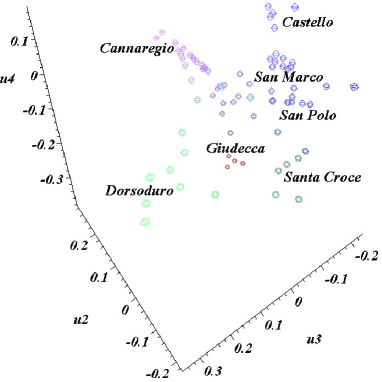
Figure 3: The segmentation of the dual graph of Venetian canals using three eigenvectors $\left[\psi_{2},\psi_{3},\psi_{4}\right]$. The nodes of dual graph can be partitioned into classes which can be almost precisely identified with the historical divisions of Venice.

In Fig. 3, we have presented the results of segmentation for the dual graph of Venetian canals using the eigenvectors $\left[\,\psi_{2},\psi_{3},\psi_{4}\,\right]$ belonging to the primary eigenvalues $1\,>\,\mu_{2}\,>\,\mu_{3}\,>\mu_{4}$. Nodes of the dual graph belonging to one and the same city district developed in a certain historical epoch are located on one and the same quasi-surface in the Euclidean space established by random walks.

Primary eigenvectors of Markov’s transition operator defined on the dual graph representation of a network indicate the directions in which the equilibrium flows have maximal ”extensions”. The use of these eigenvectors as a basis helps us to divide the nodes of the dual graph into classes which can be almost precisely identified with the historical city districts. Let us note that the implementation of other eigenvectors as the basis for the 3D representations of the dual graph worsens the quality of segmentation in a sense that it turns to be incompatible with the traditional sestieri of Venice. The slowest modes of diffusion process described by the primary eigenvectors allow detecting city modules of different accessibility.

Due to the proper normalization, the components of eigenvectors play the role of the Participation Ratios (PR) which quantify the effective numbers of nodes participating in a given eigenvector with a significant weight. This characteristic has been used in [20] and by other authors to describe the modularity of complex networks. However, PR is not a well defined quantity in the case of eigenvalue multiplicity since the different vectors in the eigenspace corresponding to the degenerate mode would obviously have different PR.

5 Graph Partitioning by Random Walks

Visual segmentation of networks based on 3D representations of their dual graphs is not always feasible. Furthermore, the result of such a segmentation may essentially depend on which eigenvectors have been chosen as the basis for the 3D representation. The computation of eigenvectors for large matrices can be time and resource consuming, and therefore it is important to have a good estimation on the minimal number of eigenvectors required for the proper graph segmentation.

The graph partitioning problem seeks to partition a weighted undirected graph $G$ into $n$ weakly connected components $\Gamma_{1},\ldots\Gamma_{n}$ such that $\bigcup_{i=1}^{n}\Gamma_{n}\subset G$ and either their properties share some common trait or the graphs nodes belonging to them are close to each other according to some distance measure defined on nodes of the graph. A number of different graph partitioning strategies for undirected weighted graphs have been studied in connection with Object Recognition and Learning in Computer Vision [21].

In Ec. 3, we have shown that random walks being introduced on a connected undirected graph $G$ establish the $(N-1)$-dimensional Euclidean space in which every pair of nodes, $i$ and $j$, appear at some distance

$$\mathrm{dist}_{T}(i,j)\,=\,\sqrt{K_{i,j}}$$ (20)

where $K_{i,j}$ is the commute time (19) of random walks between $i$ and $j$. The random walks distance (20) can be used as a measure of similarity between any two nodes in $G$. Namely, every node $i\in V$ of an undirected graph $G$ may be represented by a vector ${\bf z}^{(i)}\,\in\,\mathbb{R}^{\,(N-1)}$ in the $(N-1)$-dimensional Euclidean space associated to random walks,

$${\bf z}^{(i)}\,=\,\left(\frac{\psi_{2,i}}{\sqrt{\pi_{i}\,\left(1-\mu_{2}\right)}},\ldots,\frac{\psi_{N,i}}{\sqrt{\pi_{i}\,\left(1-\mu_{N}\right)}}\right).$$ (21)

We then assign each vector (21) to one of $n$ clusters, $\Gamma_{l}$ whose center (centroid),

$${\bf m}^{(l)}\,=\,\frac{1}{\left|\Gamma_{l}\right|}\,\sum_{j=1}^{\left|\Gamma_{l}\right|}\,{\bf z}^{(j)},$$ (22)

is the nearest to ${\bf z}^{(i)}$ with respect to the distance (20). The objective we try to achieve is to minimize the total intra-cluster variance of the resulting partition $\mathcal{P}$ of the graph $G$ into $n$ clusters, the squared error function (s.e.f.),

$$\mathrm{sef}(\mathcal{P})\,=\,\sum_{l=1}^{n}\,\sum_{s=1}^{\left|\Gamma_{l}\right|}\,\left|\,z_{s}^{(l)}-{\bf m}^{(l)}\,\right|^{2}.$$ (23)

If we denote the $(N-1)$-dimensional unity vector by ${\bf e}=(1,1,\ldots,1)^{\top}$ and ${\bf Z}\,=\,\left[{\bf z}^{(1)},\ldots{\bf z}^{(N)}\right]$ is the $N\times(N-1)$-matrix of coordinates the node acquire in the Euclidean space associated to random walks, then it is clear that

$$\begin{array}[]{lcl}\mathrm{sef}\left(\mathcal{P}\right)&=&\sum_{l=1}^{n}\,\left|\,{\bf Z}-{\bf m}^{(l)}{\bf e}^{\top}\,\right|^{2}\\ &=&\sum_{l=1}^{n}\,\left|\,{\bf Z}-{\bf P}_{l}\,\right|^{2},\end{array}$$ (24)

where ${\bf P}_{l}\,=\,\left({\bf 1}_{\Gamma_{l}}\,-\,\frac{{\bf e\,e}^{\top}}{\left|\Gamma_{l}\right|}\right)$ is the projection operator of nodes onto the cluster $\Gamma_{l}$. Since ${\bf P}_{l}^{2}\,=\,{\bf P}_{l}$, we immediately obtain that

$$\begin{array}[]{ll}\mathrm{sef}\left(\mathcal{P}\right)&=\sum_{l=1}^{n}\,\mathrm{tr}\,\left({\bf Z}^{\top}{\bf P}_{l}{\bf Z}\right)\\ &=\mathrm{tr}\,\left({\bf Z}^{\top}{\bf Z}\right)\,-\,\mathrm{tr}\,\left({\bf X}^{\top}{\bf Z}^{\top}\,{\bf Z}{\bf X}\,\right),\end{array}$$ (25)

in which

$${\bf X}=\left[\frac{\chi^{1}}{\sqrt{\left|\Gamma_{1}\right|}},\ldots,\frac{\chi^{\,n}}{\sqrt{\left|\Gamma_{n}\right|}}\right]$$ (26)

is the rectangular orthogonal $n\times N$-matrix $\left({\bf X}^{\top}{\bf X}\,=\,{\bf 1}\right)$ of the normalized indicator vectors

$$\chi^{l}_{i}\,=\,\left\{\begin{array}[]{ll}1,&i\,\in\,\Gamma_{l},\\ 0,&i\,\notin\,\Gamma_{l}.\end{array}\right.$$ (27)

Considering elements of the ${\bf Z}^{\top}{\bf Z}$ matrix as measuring similarity between nodes, we can show following [22] that the Euclidean distance (20) leads to Euclidean inner-product similarity which can be replaced by a general Mercer kernel [23, 24] uniquely represented by a positive semi-definite matrix $K_{i,j}$.

If we then relax the discrete structure of $\bf X$ by assuming that $\bf X$ is an arbitrary orthonormal matrix, the minimization of the objective function $\mathrm{sef}(\mathcal{P})$ is reduced to the trace maximization problem,

$$\max_{{\bf X}^{\top}{\bf X}\,=\,{\bf 1}_{\,N-1}}\,\,\mathrm{tr}\left(\,{\bf X}^{\top}\,{\bf Z}^{\top}{\bf Z}\,{\bf X}\,\right).$$ (28)

A standard result in linear algebra (proven by K.Fan in 1949 [25]) provides a global solution to the trace optimization problem: Given a symmetric matrix ${\bf S}$ with eigenvalues $\lambda_{1}\geq\ldots\geq\lambda_{n}\geq\ldots\geq\lambda_{N}$, and the matrix of corresponding eigenvectors, $\left[\,{\bf u}_{1},\ldots,{\bf u}_{N}\,\right]$, the maximum of $\mathrm{tr}\,\left(\,{\bf Q}^{\top}{\bf S}{\bf Q}\,\right)$ over all $n$-dimensional orthonormal matrices $\bf Q$ such that ${\bf Q}^{\top}{\bf Q}\,=\,{\bf 1}_{n}$ is given by

$$\max_{{\bf Q}^{\top}{\bf Q}\,=\,{\bf 1}_{n}}\,\,\mathrm{tr}\,\left(\,{\bf Q}^{\top}{\bf S}{\bf Q}\,\right)\,=\,\sum_{k=1}^{n}\,\lambda_{k},$$ (29)

and the optimal $n$-dimensional orthonormal matrix

$${\bf Q}\,=\,\left[\,{\bf u}_{1},\ldots,{\bf u}_{n}\,\right]{\bf R}$$ (30)

where ${\bf R}$ is an arbitrary orthogonal $n\times n$ matrix (describing a rotation transformation in $\mathbb{R}^{n}$).

The result (29-30) relates the problem of network segmentations to the investigation of $n$ primary eigenvectors of a symmetric matrix defined on the graph nodes, [26, 27]. The eigenvectors ${\bf u}_{\,i\,>\,1}$ have both positive and negative entries, so that in general the matrix $\left[\,{\bf u}_{1},\ldots,{\bf u}_{n}\,\right]$ differs substantially from that one comprising of the discrete cluster indicator vectors which have strictly positive entries.

It is important to note that even for not very large $n$ it may be rather difficult to compute the appropriate $n\,\times\,n$ orthonormal transformation matrix $\bf R$ which recovers the necessary discrete cluster indicator structures. Furthermore, it can be shown that the postprocessing of eigenvectors into the cluster indicator vectors can be reduced to an optimization problem with $n(n-1)/2\,-\,1$ parameters [28]. Several methods have been proposed to obtain the partitions from the eigenvectors of various similarity matrices (see [29],[30] for a review). In the next section, we use the ideas of Principal Component Analysis (PCA) in order to bypass the orthonormal transformation.

6 Principal Component Analysis of Venetian Canals

In statistics, Principal Component Analysis (PCA) is used for the reducing size of a data set. It is achieved by the optimal linear transformation retaining the subspace that has largest variance (a lower-order principal component) and ignoring higher-order ones [31, 32].

Given an operator $S$ self-adjoint with respect to the measure $m$ defined on a connected undirected graph $G$, it is well known that the eigenvectors of the symmetric matrix ${\bf S}$ form an ordered orthonormal basis $\left\{\,\phi_{k}\,\right\}$ with real eigenvalues $\mu_{1}\geq\ldots\geq\mu_{N}$. The ordered orthogonal basis represents the directions of the variances of variables described by $S$.

If we consider the Laplace operator, $L\,=\,1-T,$ defined on $G$, its eigenvalues can be interpreted as the inverse characteristic time scales of the diffusion process such that the smallest eigenvalues correspond to the stationary distribution together with the slowest diffusion modes involving the most significant amounts of flowing commodity. Therefore, while describing a network by means of the Laplace operator, we must arrange the eigenvalues in increasing order, $\lambda_{1}\leq\ldots\leq\lambda_{n}\leq\ldots\leq\lambda_{N}$, and examine the ordered orthogonal basis of eigenvectors, $\left[\,{\bf f}_{1},\ldots{\bf f}_{N}\,\right]$.

The number of components which may be detected in a network with regard to a certain dynamical process defined on that depends upon the number of essential eigenvectors of the relevant self-adjoint operator. There is a simple time scale argument which we use in order to determine the number of applicable eigenvectors.

It is obvious that while observing the network close to an equilibrium state during short time, we detect flows resulting from a large number of transient processes evolving toward the stationary distribution and being characterized by the relaxation times $\propto\lambda^{-1}_{k}$. While measuring the flows in sufficiently long time $\tau$, we may discover just $n$ different eigenmodes, such that

$$\lambda_{1}\,<\,\ldots\,\leq\,\lambda_{n}\,\leq\,\tau^{\,-1}\,<\,\ldots\,\leq\,\lambda_{N}.$$ (31)

In general, the longer is the time of measurements $\tau$, the less is the number of eigenvectors we have to take into account in network component analysis of the network. Should the time of measurements is fixed, we can determine the number of required eigenvectors.

In the what-following, we consider the symmetric (”normalized”) Laplace operator, [19],

$$\widehat{L_{ij}}\,=\,\delta_{ij}-\widehat{T_{ij}},$$ (32)

where $\widehat{T_{ij}}$ is the symmetric Markov transition operator (9).

6.1 Low dimensional representations of transport networks by the principal directions

In order to obtain the best quality segmentation, it is convenient to center the $n$ primary eigenvectors. The centroid vector (representing the center of mass of the set $\left[\,{\bf f}_{1},\ldots{\bf f}_{n}\,\right]$) is calculated as the arithmetic mean,

$${\bf m}\,=\,\frac{1}{n}\,\sum_{k=1}^{n}\,{\bf f}_{k}.$$ (33)

Let us denote the $n\,\times\,N$ matrix of $n$ centered eigenvectors by

$${\bf F}\,=\,\left[\,{\bf f}_{1}\,-\,{\bf m},\ldots\,{\bf f}_{N}\,-\,{\bf m}\right].$$

Then, the symmetric matrix of covariances between the entries of eigenvectors $\{{\bf f}_{k}\}$ is the product of ${\bf F}$ and its adjoint ${\bf F}^{\top}$,

$$\mathrm{\bf Cov}\,=\,\frac{\,\,{\bf F}\,{\bf F}^{\top}\,}{N\,-\,1}$$ (34)

It is important to note that the correspondent Gram matrix ${\bf F}^{\top}\,{\bf F}\,/(N-1)\,\equiv\,{\bf 1}$ due to the orthogonality of the basis eigenvectors.

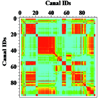
Figure 4: The correlation matrix calculated for the dual graph representation of Venetian canals calculated for the system of the first 7 eigenvectors of the normalized Laplace operator (32). The entries of the matrix are ranked from 1 (red) to -1 (blue).

The main contributions in the symmetric matrix $\mathrm{\bf Cov}$ are related to the groups of nodes

$$\mathrm{\bf Cov}{\ }{\bf u}_{k}\,=\,\sigma_{k}\,{\bf u}_{k},$$ (35)

which can be identified by means of the eigenvectors $\{\,{\bf u}_{k}\,\}$ associated to the first largest eigenvalues among $\sigma_{1}\,\geq\,\sigma_{2},$ $\dots,\,\geq\,\sigma_{N}$. By ordering the eigenvectors in decreasing order (largest first), we create an ordered orthogonal basis with the first eigenvector having the direction of largest variance of the components of $n$ eigenvectors $\{{\bf f}_{k}\}$. Let us note that due to the structure of ${\bf F}$ only the first $n-1$ eigenvalues $\sigma_{k}$ are not trivial. In accordance to the standard PCA notation, the eigenvectors of the covariance matrix ${\bf u}_{k}$ are called the principal directions of the network with respect to the diffusion process defined by the operator $S$. A low dimensional representation of the network is given by its principal directions $\left[\,{\bf u}_{1},\ldots,{\bf u}_{n-1}\,\right],$ for $n\,<\,N$.

Diagonal elements of the matrix $\mathrm{\bf Cov}$ quantify the component variances of the eigenvectors $\left[\,{\bf f}_{1},\ldots{\bf f}_{n}\,\right]$ around their mean values (33) and may be ample essentially for large networks. Therefore, it is practical for us to use the standardized correlation matrix,

$${\mathrm{C}orr}_{ij}\,=\,\frac{\mathrm{Cov}_{ij}}{\sqrt{\mathrm{Cov}_{ii}}\sqrt{\mathrm{Cov}_{jj}}},$$ (36)

instead of the covariance matrix ${\mathrm{\bf Cov}}$. It is important to note that the diagonal elements of (36) equal 1, while the off-diagonal elements are the Pearson’s coefficients of linear correlations, [33].

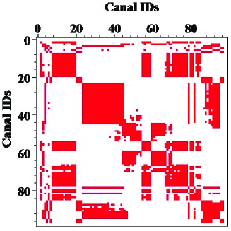
Figure 5: The coarse-grained connectivity matrix derived from the low-dimensional representation of Venetian canals given by the transition matrix ${\bf U}_{6}\,{\bf U}_{6}^{\top}$.

The correlation matrix (36) calculated with regard to the first $n$ eigenvectors possesses a complicated structure containing the multiple overlapping blocks pertinent to a low-dimensional representation of the network of Venetian canals which allows for a further simplification. In Fig. 4, we have presented the correlation matrix (36) figured out for the first 7 eigenvectors of the normalized Laplace operator (32) defined on the dual graph representation of 96 Venetian canals.

Let ${\bf U}$ be the orthonormal matrix which contains the eigenvectors $\{{\bf u}_{k}\}$, $k\,=\,1,\ldots,\,n-1,$ of the covariance (or correlation) matrix as the row vectors. These vectors form the orthogonal basis of the $(n-1)$-dimensional vector space, in which every variance $({\bf f}_{k}-{\bf m})$ is represented by a point ${\bf g}_{k}\,\in\,\mathbb{R}^{\,(n-1)}$,

$${\bf g}_{k}\,=\,{\bf U}\,({\bf f}_{k}-{\bf m}\,).$$ (37)

Then each original eigenvector ${\bf f}_{k}$ can be decoded from ${\bf g}_{k}\,\in\,\mathbb{R}^{\,(n-1)}$ by the inverse transformation,

$${\bf f}_{k}\,=\,{\bf U}^{\top}\,{\bf g}_{k}\,+\,{\bf m}.$$ (38)

The use of transformations (37) and (38) allows to obtain the $(n-1)$-dimensional representation $\left\{\,\varphi_{k}\,\right\}_{\,k=1}^{\,(n-1)}$ of the $N$-dimensional basis vectors $\left\{\,{\bf f}_{s}\,\right\}_{\,s=1}^{\,N}$ in the form

$$\varphi_{\,k}\,=\,{\bf U}^{\top}{\bf U}\,{\bf f}_{k}\,+\,\left(\,{\bf 1}-{\bf U}^{\top}{\bf U}\,\right)\,{\bf m},$$ (39)

that minimizes the mean-square error between ${\bf f}_{k}\,\in\,\mathbb{R}^{\,N}$ and $\varphi_{k}\,\in\,\mathbb{R}^{\,(n-1)}$ for given $n$.

Variances of eigenvectors $\left\{\,{\bf f}_{k}\,\right\}$ are positively correlated within a principal component of the transport network. Thus, the transition matrix ${\bf U}^{\top}{\bf U}$ can be interpreted as the connectivity patterns acquired by the network with respect to the diffusion process. Two nodes, $i$ and $j$, belong to one and the same principal component of the network if $\left({\bf U}{\bf U}^{\top}\right)_{ij}\,>\,0$. By applying the Heaviside function, which is zero for negative argument and one for positive argument, to the elements of the transition matrix ${\bf U}{\bf U}^{\top}$, we derive the coarse-grained connectivity matrix of network components. In Fig. 5, we have shown the coarse-grained connectivity matrix obtained from the transition matrix ${\bf U}_{6}\,{\bf U}_{6}^{\top}$ for the dual graph representation of Venetian canals.

6.2 Dynamical segmentations of transport networks

In general, the building of low-dimensional representations for transport networks with respect to a certain dynamical process defined on them is a complicated procedure which cannot be reduced to (and reproduced by) the naive introduction of ”supernodes” by either merging of several nodes or shrinking complete subgraphs of the original graph. The implementation of spectral approach removes indeterminacies of the empirical clique concatenation techniques used in space syntax analysis of urban textures, [34]. If the covariance matrix clearly exhibits a block structure, and once the relevant coarse-grained connectivity matrix is computed, we can identify dynamical clusters (blocks) by using a linearized cluster assignment and compute the cluster crossing, the cluster overlap along the specified ordering using the spectral ordering algorithm, [28].

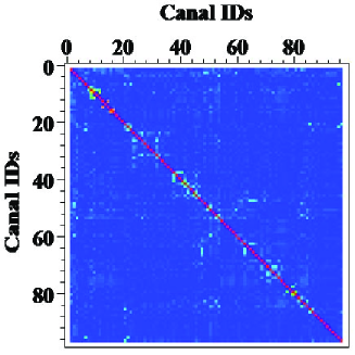
Figure 6: The covariance matrix calculated for the dual graph representation of Venetian canals with regrades to the first 80 eigenvectors of the normalized Laplace operator (32). The entries of covariance matrix are ranked from the largest positive values (red) to the utmost negative values (blue).

The problem of dynamical segmentations of a transport network in fast time scales is more computationally complex especially for large networks, because of many eigenvectors if not all have to be taken into account while calculating the covariance matrix. It is important to note that the covariance matrix in this case takes the form of a sparse, nearly diagonal matrix (see Fig. 6).

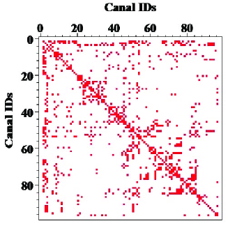
Figure 7: The fast time scale coarse-grained connectivity matrix for the low-dimensional representation of Venetian canals deduced from the transition matrix ${\bf U}_{79}\,{\bf U}_{79}^{\top}$.

Sparsity of the deduced coarse-grained connectivity matrix (which is shown in Fig. 7) in fast time scales entails loosely coupled systems lack any form of large scale structure. A sparse coarse-grained connectivity matrix may be useful when storing and manipulating data for approximate descriptions of transport networks in fast time scales.

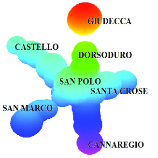
Figure 8: The 3D-image of a dynamical segmentation of Venetian canals built for the first 8 eigenvalues of the normalized Laplace operator (32). The structural differences between the historical city districts of Venice are clearly visible.

Low-dimensional representations of not very large transport networks given by the coarse-grained connectivity matrices can be represented by a 3D-graph. In Fig. 8, we have shown the 3D-image of a dynamical segmentation of Venetian canals. The dual graph representation of the Venetian canal network has been analyzed, and a ball has been assigned to each canal. The radius of the $i^{\mathrm{th}}$-ball is taken equal to the norm (16), the node $i$ has in the $(N-1)$-dimensional Euclidean space associated to random walks introduced on the connected, undirected dual graph of Venetian canals,

$$r_{i}\,=\,\|\upsilon_{i}\|_{T}$$ (40)

Those nodes characterizing by the worst accessibility levels have the largest norms with respect to random walks and therefore are represented by balls of the largest radiuses.

The coordinates of each ball have been given by the relevant components of the first three eigenvectors of the coarse-grained connectivity matrix displayed in Fig. 5. These eigenvectors determine the directions of the largest variances of correlations delineating the low-dimensional representation of the network. The key observation is that canals with short access times are also characterized by small variances of correlations, therefore being forgathered proximate to the center of the figure displayed in Fig. 8, no matter which city district they belong to. In the contrary, the worst accessible canals are distinguished by the strongest correlation variances and are located on the figure fringes, far apart from its center. At the same time, the radiuses of the balls representing them are the largest among all other balls since they acquire the utmost norms with respect to random walks. It is remarkable that they can be perfectly identified with the traditional historical sestieri of Venice.

7 Discussion and Conclusion

The impact of urban landscapes on the construction of social relations draws attention in the fields of ethnography, sociology, and anthropology. In particular, it has been suggested that the urban space combining social, economic, ideological and technological factors is responsible for the technological, socioeconomic, and cultural development, [35]. It is worth to mention that the processes relating urbanization to economic development and knowledge production are very general, being shared by all cities belonging to the same urban system and sustained across different nations and times [36]. There is a tied connection between physical activity of humans, their mobility and the layout of buildings, roads, and other structures that physically define a community [37]. Spatial organization of a place has an extremely important effect on the way people move through spaces and meet other people by chance [38]. The patterns of social movement and economical development for a thousand years of Venetian history have been imprinted in space syntax of the city.

In the present paper, we have investigated the canal network in Venice by means of random walks. Random walks being defined on an undirected graph of $N$ modes, establish the $(N-1)$- dimensional Euclidean space in which distances and angles acquire the clear statistical interpretation. The properties of nodes with respect to random walks allow partitioning the city canal network into disjoint divisions which may be identified with the traditional divisions of Venice (sestieri).

We have developed the general approach to the coarse-graining of transport networks based on the PCA method for the low-dimensional representation of large data set. We believe that the proposed technique can be useful in many applications potential applications such as the establishing of rigorous mathematical foundations for the analysis of urban textures establishing the urbanization road to a harmonious city.

8 Acknowledgment

The work has been supported by the Volkswagen Foundation (Germany) in the framework of the project: ”Network formation rules, random set graphs and generalized epidemic processes” (Contract no Az.: I/82 418). The authors acknowledge the multiple fruitful discussions with the participants of the workshop Madeira Math Encounters XXXIII, August 2007, CCM - CENTRO DE CIÊNCIAS MATEMÁTICAS, Funchal, Madeira (Portugal).

References

- [1] D. Volchenkov, Ph. Blanchard, Phys. Rev. E 75, 026104 (2007).
- [2] N. Biggs, E. Lloyd, and R. Wilson, Graph Theory, 1736-1936. Oxford University Press (1986).
- [3] P. Haggett, R. Chorley (eds.), Socio-Economic Models in Geography, London, Methuen (1967). P. Haggett, R. Chorley, Network Analysis in Geography, Edward Arnold, London (1969).
- [4] K.J. Kansky, Structure of Transportation Networks: Relationships Between Network Geometry and Regional Characteristics, Research Paper 84, Department of Geography, University of Chicago , Chicago, IL (1963).
- [5] H.J. Miller, S.L. Shaw, Geographic Information Systems for Transportation: Principles and Applications, Oxford Univ. Press, Oxford (2001).
- [6] M. Batty, A New Theory of Space Syntax, UCL Centre For Advanced Spatial Analysis Publications, CASA Working Paper 75 (2004).
- [7] B. Hillier, A. Leaman, P. Stansall, M. Bedford, Environment and Planning B 3, 147-185 (1976).
- [8] B. Hillier, Space is the machine. A configurational theory of architecture, Cambridge University Press (1996).
- [9] B. Jiang, ”A space syntax approach to spatial cognition in urban environments”, Position paper for NSF-funded research workshop Cognitive Models of Dynamic Phenomena and Their Representations, October 29 - 31, 1998, University of Pittsburgh, Pittsburgh, PA (1998).
- [10] C. Ratti, Environment and Planning B: Planning and Design, vol. 31, pp. 487 - 499 (2004).
- [11] M.J.T. Kruger, On node and axial grid maps: distance measures and related topics. Other. Bartlett School of Architecture and Planning, UCL, London, UK (1989).
- [12] S. Skiena, Implementing Discrete Mathematics: Combinatorics and Graph Theory with Mathematica, Reading, MA: Addison-Wesley (1990).
- [13] J.G. Wardrop, Proc. of the Institution of Civil Engineers 1 (2), pp. 325-362 (1952).
- [14] M.J. Beckmann, C.B. McGuire, C.B. Winsten, Studies in the Economics of Transportation. Yale University Press, New Haven, Connecticut (1956).
- [15] S. Lim, Minimal Volume Entropy on Graphs. Preprint arXiv:math.GR/050621, (2005).
- [16] A. Smola and R. I. Kondor. ”Kernels and regularization on graphs”. In Learning Theory and Kernel Machines, Springer (2003).
- [17] D.J. Aldous, J.A. Fill, Reversible Markov Chains and Random Walks on Graphs. A book in preparation, available at www.stat.berkeley.edu/aldous/book.html.
- [18] L. Lovász, Bolyai Society Mathematical Studies 2: Combinatorics, Paul Erdös is Eighty, Keszthely (Hungary), p. 1-46 (1993).
- [19] F. Chung, Lecture notes on spectral graph theory, AMS Publications Providence (1997).
- [20] K. A. Eriksen, I. Simonsen, S. Maslov, K. Sneppen, Phys. Rev. Lett. 90 (14), id. 148701 (2003).
- [21] T. Morris, Computer Vision and Image Processing. Palgrave Macmillan. ISBN 0-333-99451-5 (2004).
- [22] H. Zha, C. Ding, M. Gu, X. He and H. Simon, Neural Information Processing Systems 14 (NIPS 2001), pp. 1057-1064, Vancouver, Canada (2001).
- [23] S. Saitoh, Theory of Reproducing Kernels and its Applications, Longman Scientific and Technical, Harlow, UK (1988).
- [24] G. Wahba, Spline Models for Observational Data 59 of CBMS-NSF Regional Conference Series in Applied Mathematics, SIAM, Philadelphia (1990).
- [25] K. Fan, Proc. Natl. Acad. Sci. USA 35, 652-655 (1949).
- [26] G. Golub, C. van Loan,Matrix computations, 3rd edition, The Johns Hopkins University Press, London (1996).
- [27] I. Dhillon, Y. Guan, and B. Kulis, ”Kernel k-means: spectral clustering and normalized cuts”, in Proceedings of the 10th ACM SIGKDD international conference on Knowledge discovery and data mining, Seattle, WA, USA (2004).
- [28] C. Ding, X. He, Proc. of Intl. Conf. Machine Learning (ICML’2004), 225-232. July 2004.
- [29] I. Dhillon, Y. Guan, and B. Kulis, ”A unified view of kernel k-means, spectral clustering and graph cuts”. Technical Report TR-04-25, University of Texas at Austin (2004), available at http://www.cs.utexas.edu/users/kulis/pubs/spectral_techreport.pdf.
- [30] F. R. Bach, M. I. Jordan, ”Learning spectral clustering”, Technical report, UC Berkeley, available at www.cs.berkeley.edu/fbach (2003); Tutorial given at ICML 2004 International Conference on Machine Learning, Banff, Alberta, Canada (2004).
- [31] K. Fukunaga, Introduction to Statistical Pattern Recognition, ISBN 0122698517, Elsevier (1990).
- [32] I.T. Jolliffe, Principal Component Analysis (2-nd edition) Springer Series in Statistics (2002).
- [33] J. Cohen, P. Cohen, S.G. West, L.S. Aiken, Applied multiple regression/correlation analysis for the behavioral sciences. (3rd ed.) Hillsdale, NJ: Lawrence Erlbaum Associates (2003).
- [34] R.C. Dalton, S. Bafna, The syntactical image of the city : A reciprocal definition of spatial elements and spatial syntaxes. In 4th International Space Syntax Symposium, London (2003).
- [35] S. Low, L. Zuniga (eds.), The Anthropology of Space and Place: Locating Culture, Blackwell Publishing (2003).
- [36] L.M.A. Bettencourt, J. Lobo, D. Helbing, C. Kühnert, and G.B. West, ”Growth, innovation, scaling, and the pace of life in cities”, PNAS published online Apr 16, 2007; doi:10.1073/pnas.0610172104.
- [37] Does the Built Environment Influence Physical Activity? Examining the Evidence – Special Report from the USNational Academies’ Transportation Research Board and US Institute of Medicine 282 (2005).
- [38] B. Hillier, J. Hanson, The Social Logic of Space (1993, reprint, paperback edition ed.). Cambridge: Cambridge University Press (1984).