Nonlinear Neumann boundary stabilization
of the wave equation using rotated multipliers.

Abstract

We study the boundary stabilization of the wave equation by means of a linear or non-linear Neumann feedback. The rotated multiplier method leads to new geometrical cases concerning the active part of the boundary where the feedback is applied. Due to mixed boundary conditions, these cases generate singularities. Under a simple geometrical condition concerning the orientation of the boundary, we obtain stabilization results in both cases.

AMS Subject Classification: 93D15, 35L05, 35J25

Introduction

In this paper we are concerned with the stabilization of the wave equation in a multi-dimensional body $\Omega\subset{\mathbb{R}}^{n}$ by using a feedback law applied on some part of its boundary. The problem can be written as follows

$$\left\{\begin{matrix}u^{\prime\prime}-\Delta u=0\quad&\text{in }\Omega\times\mathbb{R}^{*}_{+}\,,\hfill\\ u=0\hfill&\text{on }\partial\Omega_{D}\times\mathbb{R}^{*}_{+}\,,\hfill\\ \partial_{\nu}u=F\hfill&\text{on }\partial\Omega_{N}\times\mathbb{R}^{*}_{+}\,,\hfill\\ u(0)=u_{0}\hfill&\text{in }\Omega\,,\hfill\\ u^{\prime}(0)=u_{1}\hfill&\text{in }\Omega\,,\hfill\end{matrix}\right.$$

where we denote by $u^{\prime}$, $u^{\prime\prime}$, $\Delta u$ and $\partial_{\nu}u$ the first time-derivative of $u$, the second time-derivative of the scalar function $u$, the standard Laplacian of $u$ and the normal outward derivative of $u$ on $\partial\Omega$, respectively; $(\partial\Omega_{D}$, $\partial\Omega_{N})$ is a partition of $\partial\Omega$ and $F$ is the feedback function which may depend on the state $(u,u^{\prime})$, the position ${\mathbf{x}}$ and time $t$.
Our purpose here is to choose the feedback function $F$ and the active part of the boundary, $\partial\Omega_{N}$, so that for every initial data, the energy function

$$E(u,t)=\frac{1}{2}\int_{\Omega}(|u^{\prime}(t)|^{2}+|\nabla u(t)|^{2})\,d{\mathbf{x}}\,,$$

is decreasing with respect to time $t$, and vanishes as $t\longrightarrow\infty$.
Formally, we can write the time derivative of $E$ as follows

$$E^{\prime}(u,t)=\int_{\partial\Omega_{N}}Fu^{\prime}\,d\sigma\,,$$

and a sufficient condition so that $E$ is non-increasing is  $Fu^{\prime}\leq 0$ on $\partial\Omega_{N}$.
In the two-dimensional case and in the framework of Hilbert Uniqueness Method [11], it can be shown that the energy function is uniformly decreasing as $t$ tends to $\infty$, by choosing   ${\mathbf{m}}:{\mathbf{x}}\mapsto{\mathbf{x}}-{\mathbf{x}}_{0}$, where ${\mathbf{x}}_{0}$ is some given point in ${\mathbb{R}}^{n}$ and

$$\partial\Omega_{N}=\left\{{\mathbf{x}}\in\partial\Omega\,/\,m({\mathbf{x}}).\nu({\mathbf{x}})>0\,\right\}\,,\quad F=-{\mathbf{m}}.{\boldsymbol{\nu}}\,u^{\prime}\,,$$

where ${\boldsymbol{\nu}}$ is the normal unit vector pointing outward of $\Omega$. This method has been performed by many authors, see for instance [10] and references therein. Here we extend the above result for rotated multipliers [15, 16] by following [4], i.e. we take in account singularities which can appear when changing boundary conditions along the interface $\Gamma=\overline{\partial\Omega_{N}}\cap\overline{\partial\Omega_{D}}$.

1 Notations and main results

Let $\Omega$ be a bounded open connected set of $\mathbb{R}^{n}(n\geq 2)$ such that

$$\partial\Omega\text{ is of class }\mathcal{C}^{2}\text{ in the sense of Ne\v{c}as \cite[cite]{[\@@bibref{}{Ne}{}{}]}}.$$ (1)

Let ${\mathbf{x}}_{0}$ be a fixed point in $\mathbb{R}^{n}$. We denote by $I$ the $n\times n$ identity matrix, by $A$ a real $n\times n$ skew-symmetric matrix and by $d$ a positive real number such that $d^{2}+\|A\|^{2}=1$,where $\|\cdot\|$ stands for the usual $2$-norm of matrices. We now define the following vector function,

$$\forall{\mathbf{x}}\in\mathbb{R}^{n},\quad{\mathbf{m}}({\mathbf{x}})=(dI+A)({\mathbf{x}}-{\mathbf{x}}_{0})\,.$$

We consider a partition $(\partial\Omega_{N},\partial\Omega_{D})$ of $\partial\Omega$ such that

$$\left|\begin{array}[]{l}\Gamma=\overline{\partial\Omega_{D}}\cap\overline{\partial\Omega_{N}}\text{\ is a }\mathcal{C}^{3}\text{-manifold of dimension }n-2,\\ {\mathbf{m}}.{\boldsymbol{\nu}}=0\text{ on }\Gamma,\\ \partial\Omega\cap\omega\ \text{\ is a }\mathcal{C}^{3}\text{-manifold of dimension }n-1,\\ \mathcal{H}^{n-1}(\partial\Omega_{D})>0,\end{array}\right.$$ (2)

where $\omega$ is a suitable neighborhood of $\Gamma$ and $\mathcal{H}^{n-1}$ denotes the usual $(n-1)$-dimensional Hausdorff measure.

Let $g:$ $\mathbb{R}\rightarrow\mathbb{R}$ be a measurable function such that

$$g\text{ is non-decreasing}\quad\text{and}\quad\exists K>0\,:\quad|g(s)|\leq K|s|\,\text{ a.e..}$$ (3)

Let us now consider the following wave problem

$$(S)\,\left\{\begin{array}[]{l}u^{\prime\prime}-\Delta u=0\\ u=0\\ \partial_{\nu}u=-{\mathbf{m}}.{\boldsymbol{\nu}}\,g(u^{\prime})\\ u(0)=u_{0}\\ u^{{}^{\prime}}(0)=u_{1}\end{array}\right.\left.\begin{array}[]{l}\text{ in }\Omega\times\mathbb{R}_{+}^{\ast},\\ \text{ on }\partial\Omega_{D}\times\mathbb{R}_{+}^{\ast},\\ \text{ on }\partial\Omega_{N}\times\mathbb{R}_{+}^{\ast},\\ \text{ in }\Omega,\\ \text{ in }\Omega,\end{array}\right.$$

for some initial data

$$(u_{0},u_{1})\in\mathrm{H}_{D}^{1}(\Omega)\times\mathrm{L}^{2}(\Omega):=\mathrm{H}$$

with $\mathrm{H}_{D}^{1}(\Omega)=\{v\in\mathrm{H}^{1}(\Omega)\,/\,v=0\text{ on }\partial\Omega_{D}\}$.

This problem is well-posed in $\mathrm{H}$. Indeed, following Komornik [9], we define the non-linear operator $\mathcal{A}$ by

$$\left.\begin{array}[]{l}\mathcal{A}(u,v)=(-v,-\Delta u),\\ D(\mathcal{A})=\{(u,v)\in\mathrm{H}_{D}^{1}(\Omega)\times\mathrm{H}_{D}^{1}(\Omega)\,/\,\Delta u\in\mathrm{L}^{2}(\Omega)\text{\, and \, }\partial_{\nu}u=-{\mathbf{m}}.{\boldsymbol{\nu}}\,g(v)\,\text{ on }\partial\Omega_{N}\},\end{array}\right.$$

so that $(S)$ can be written in the form

$$\left\{\begin{array}[]{l}(u,v)^{\prime}+\mathcal{A}(u,v)=0\,,\\ (u,v)(0)=(u_{0},u_{1})\,.\end{array}\right.$$

It is a classical fact that $\mathcal{A}$ is a maximal-monotone operator on $\mathrm{H}$ and that $D(\mathcal{A})$ is dense in $\mathrm{H}$ for the usual norm (see for instance [1]). Hence, for any initial data $(u_{0},v_{0})\in$ $D(\mathcal{A})$ there is a unique strong solution $(u,v)$ such that $u\in\mathrm{W}^{1,\infty}(\mathbb{R};\mathrm{H}_{D}^{1}(\Omega))$ and $\Delta u\in\mathrm{L}^{\infty}(\mathbb{R}_{+};\mathrm{L}^{2}(\Omega))$. Moreover, for two initial data, the corresponding solutions satisfy

$$\forall t\geq 0\,,\quad\|(u^{1}(t),v^{1}(t))-(u^{2}(t),v^{2}(t))\|_{\mathrm{H}}\leq C\|(u^{1}_{0},v^{1}_{0})-(u^{2}_{0},v^{2}_{0})\|_{\mathrm{H}}\,.$$

Using the density of $D(\mathcal{A})$, one can extend the map

$$D(\mathcal{A}) \longrightarrow \mathrm{H}$$

$$(u_{o},v_{0}) \longmapsto (u(t),v(t))$$

to a strongly continuous semi-group of contractions $(S(t))_{t\geq 0}$ and define for $(u_{0},v_{0})\in\mathrm{H}$ the weak solution $(u(t),u^{\prime}(t))=S(t)(u_{0},u_{1})$ with the regularity $u\in\mathcal{C}(\mathbb{R}_{+};\mathrm{H}_{D}^{1}(\Omega))\cap\mathcal{C}^{1}(\mathbb{R}_{+};\mathrm{L}^{2}(\Omega))$. We hence define the energy function of solutions by

$$E(u,0)=\frac{1}{2}\int_{\Omega}(|u_{1}|^{2}+|\nabla u_{0}|^{2})\,d{\mathbf{x}},\qquad E(u,t)=\frac{1}{2}\int_{\Omega}(|u^{\prime}(t)|^{2}+|\nabla u(t)|^{2})\,d{\mathbf{x}}\quad\text{if }t>0\,.$$

In order to get stabilization results, we need further assumptions concerning the feedback function $g$

$$\exists p\geq 1\,,\ \exists k>0\,,\quad|g(s)|\geq k\min\{|s|,|s|^{p}\}\,,\ \hbox{a.e.}\,.$$ (4)

Concerning the boundary we assume

$$\partial\Omega_{N}\subset\{{\mathbf{x}}\in\partial\Omega\,/\,{\mathbf{m}}({\mathbf{x}}).{\boldsymbol{\nu}}({\mathbf{x}})\geq 0\}\,,\quad\partial\Omega_{D}\subset\{{\mathbf{x}}\in\partial\Omega\,/\,{\mathbf{m}}({\mathbf{x}}).{\boldsymbol{\nu}}({\mathbf{x}})\leq 0\},$$ (5)

and the additional geometric assumption

$${\mathbf{m}}.{\boldsymbol{\tau}}\leq 0\,\quad\text{on }\Gamma\,,$$ (6)

where ${\boldsymbol{\tau}}({\mathbf{x}})$ is the normal unit vector pointing outward of $\partial\Omega_{N}$ at a point ${\mathbf{x}}\in\Gamma$ when considering $\partial\Omega_{N}$ as a sub-manifold of $\partial\Omega$.

Remark 1

It is worth observing that it is not necessary to assume that

$$\mathcal{H}^{n-1}(\{{\mathbf{x}}\in\partial\Omega_{N}\,/\,{\mathbf{m}}({\mathbf{x}}).{\boldsymbol{\nu}}({\mathbf{x}})>0\})>0.$$

to get stabilization. In fact, our choice of ${\mathbf{m}}$ implies such properties (see examples in Section 4) whether the energy tends to zero.

Since the pioneering work [12], it is now a well-known fact that Rellich type relations [17] are very useful for the study of control and stabilization of the wave problem. As we said before, Komornik and Zuazua [10] have shown how these relations can also help us to stabilize the wave problem. In order to generalize it in higher dimension than 3, the key-problem is to show the existence of a decomposition of the solution in regular and singular parts [6, 8] which can be applied to stabilization problems or control problems. The first results towards this direction are due to Moussaoui [13], and Bey-Lohéac-Moussaoui [4] who also have established a Rellich type relation in any dimension.
In this new case of Neumann feedback deduced from [15, 16], our goal is to generalize those Rellich relations to get stabilization results about $(S)$ under assumptions (5), (6).
As well as in [9], we shall prove here two results of uniform boundary stabilization.

Exponential boundary stabilization

We here consider the case when $p=1$ in (4). This is satisfied when $g$ is linear,

$$\exists\alpha>0\,:\qquad\forall s\in\mathbb{R}\,,\quad g(s)=\alpha s\,.$$

In these cases, the energy function is exponentially decreasing.

Theorem 1

Assume that geometrical conditions (2), (5) hold and that the feedback function $g$ satisfies (3) and (4) with $p=1$.
Then under the further geometrical assumption (6), there exist $C>0$ and $T>0$ (independent of $d$) such that for all initial data in $\mathrm{H}$, the energy of the solution $u$ of satisfies

$$\forall t>\frac{T}{d}\,,\quad E(u,t)\leq E(u,0)\,\exp\Bigl{(}1-\frac{d}{C}t\Bigr{)}\,.$$

The above constants $C$ and $T$ depend only on the geometry.

Rational boundary stabilization

We here consider the general case and we get rational boundary stabilization.

Theorem 2

Assume that geometrical conditions (2), (5) hold and that the feedback function $g$ satisfies (3) and (4) with $p>1$.
Then under the further geometrical assumption (6), there exist $C>0$ and $T>0$ (independent of $d$) such that for all initial data in $\mathrm{H}$, the energy of the solution $u$ of satisfies

$$\forall t>\frac{T}{d}\,,\quad E(u,t)\leq C\,t^{2/(p-1)}\,.$$

where $C$ depends on the initial energy $E(u,0)$.

Remark 2

Taking advantage of the works of Banasiak-Roach [2] who generalized Grisvard’s results [6] in the piecewise regular case, we will see that Theorems 1 and 2 remain true in the bi-dimensional case when assumption (1) is replaced by following one

$$\begin{matrix}&\partial\Omega\text{ is a curvilinear polygon of class }{\cal C}^{2}\,,\hfill\\ &\text{each component of }\partial\Omega\setminus\Gamma\text{ is a }{\cal C}^{2}\hbox{-manifold of dimension }1\,,\\ \end{matrix}$$ (7)

and when condition (6) is replaced by

$$\begin{matrix}\forall{\mathbf{x}}\in\Gamma\,,\quad 0\leq\varpi_{\mathbf{x}}\leq\pi\quad\text{and\quad if }\varpi_{\mathbf{x}}=\pi\,,\,\,{\mathbf{m}}({\mathbf{x}}).{\boldsymbol{\tau}}({\mathbf{x}})\leq 0\,.\end{matrix}$$ (8)

where $\varpi_{\mathbf{x}}$ is the angle at the boundary in the point ${\mathbf{x}}$.

These two results are obtained by estimating some integral of the energy function as well as in [9]. This specific estimates are obtained thanks to an adapted Rellich relation.
Hence, this paper is composed of two sections. In the first one we build convenient Rellich relations and in the second one we use it to prove Theorems 1 and 2.

2 Rellich relations

2.1 A regular case

We can easily build a Rellich relation corresponding to the above vector field $m$ when considered functions are smooth enough.

Proposition 3

Assume that $\Omega$ is an open set of $\mathbb{R}^{n}$ with boundary of class $\mathcal{C}^{2}$ in the sense of Nečas. If $u$ belongs to $\mathrm{H}^{2}(\Omega)$ then

$$2\int_{\Omega}\Delta u\,({\mathbf{m}}.\nabla u)\,d{\mathbf{x}}=d\,(n-2)\int_{\Omega}|\nabla u|^{2}\,d{\mathbf{x}}+\int_{\partial\Omega}\bigl{(}2\partial_{\nu}u\,({\mathbf{m}}.\nabla u)-{\mathbf{m}}.{\boldsymbol{\nu}}\,|\nabla u|^{2}\bigr{)}\,d\sigma\,.$$

Proof. Using Green-Riemann identity we get

$$2\int_{\Omega}\Delta u\,({\mathbf{m}}.\nabla u)\,d{\mathbf{x}}=\int_{\partial\Omega}2\partial_{\nu}u\,({\mathbf{m}}.\nabla u)\,d\sigma-2\int_{\Omega}\nabla u.\nabla({\mathbf{m}}.\nabla u)\,d{\mathbf{x}}\,.$$

So, observing that

$$\nabla u.\nabla({\mathbf{m}}.\nabla u)=\frac{1}{2}{\mathbf{m}}.\nabla(|\nabla u|^{2})+d|\nabla u|^{2}+(A\nabla u).\nabla u\,,$$

and since $A$ is skew-symmetric, we get

$$2\int_{\Omega}\Delta u\,({\mathbf{m}}.\nabla u)\,d{\mathbf{x}}=\int_{\partial\Omega}2\partial_{\nu}u\,({\mathbf{m}}.\nabla u)\,d\sigma-2d\int_{\Omega}|\nabla u|^{2}\,d{\mathbf{x}}-\int_{\Omega}{\mathbf{m}}.\nabla(|\nabla u|^{2})\,d{\mathbf{x}}\,.$$

With another use of Green-Riemann formula, we obtain the required result for $\text{div}({\mathbf{m}})=nd$.   

We will now try to extend this result to the case of an element $u$ belonging less regular when $\Omega$ is smooth enough.

2.2 Bi-dimensional case

We begin by the plane case. It is the simplest case from the point of view of singularity theory and its understanding dates from Shamir [18].

Theorem 4

Assume $n=2$. Under geometrical conditions (2) and (7), let $u\in\mathrm{H}^{1}(\Omega)$ such that

$$\Delta u\in\mathrm{L}^{2}(\Omega)\,,\quad u_{/\partial\Omega_{D}}\in\mathrm{H}^{3/2}(\partial\Omega_{D})\,,\quad\partial_{\nu}u_{/\partial\Omega_{N}}\in\mathrm{H}^{1/2}(\partial\Omega_{N})\,.$$ (9)

Then $\,2\partial_{\nu}u\,({\mathbf{m}}.\nabla u)-{\mathbf{m}}.{\boldsymbol{\nu}}\,|\nabla u|^{2}$ belongs to $\mathrm{L}^{1}(\partial\Omega)$ and there exist some coefficients $(c_{{\mathbf{x}}})_{{\mathbf{x}}\in\Gamma}$ such that

$$2\int_{\Omega}\Delta u({\mathbf{m}}.\nabla u)\,d{\mathbf{x}}=\int_{\partial\Omega}(2\partial_{\nu}u\,({\mathbf{m}}.\nabla u)-{\mathbf{m}}.{\boldsymbol{\nu}}\,|\nabla u|^{2})\,d\sigma+\frac{\pi}{4}\sum_{{\mathbf{x}}\in\Gamma/\varpi_{\mathbf{x}}=\pi}c_{{\mathbf{x}}}^{2}\,({\mathbf{m}}.{\boldsymbol{\tau}})({\mathbf{x}})\,.$$

Proof. We first begin by some considerations which will be used in the general case too. It is a classical result that $u\in\mathrm{H}^{2}(\omega)$ for every open domain $\omega$ such that $\omega\Subset\overline{\Omega}\setminus\Gamma$. For sake of completeness, let us recall the proof.

A trace result shows that there exists $u_{R}\in\mathrm{H}^{2}(\omega)$ such that $u_{R}=u$ on $\partial\Omega_{D}$ and $\partial_{\nu}u_{R}=\partial_{\nu}u$ on $\partial\Omega_{N}$. Hence, setting $f=\Delta u_{R}-\Delta u\in\mathrm{L}^{2}(\Omega)$, $u_{S}=u-u_{R}$ satisfies

$$\left\{\begin{array}[]{l}-\Delta u_{S}=f\\ u_{S}=0\\ \partial_{\nu}u_{S}=0\end{array}\right.\left.\begin{array}[]{l}\text{in }\Omega\,,\\ \text{on }\partial\Omega_{D}\,,\\ \text{on }\partial\Omega_{N}\,.\end{array}\right.$$ (10)

$\bullet$ Now, if $\omega\Subset\Omega\setminus\Gamma\cup\partial\Omega_{D}$ and $\xi$ is a cut-off function such that $\xi=1$ on $\omega$ and supp$(\xi)\subset\Omega$, then for a suitable $g\in\mathrm{L}^{2}(\Omega)$, $u_{\omega}=u_{S}\xi$ satisfies the Dirichlet problem

$$\left\{\begin{array}[]{l}\Delta u_{\omega}=g\\ u_{\omega}=0\end{array}\right.\left.\begin{array}[]{l}\text{on }\Omega\,,\\ \text{on }\partial\Omega\,,\end{array}\right.$$

and using classical method of difference quotients ([6]), one can now conclude that $u_{\omega}\in\mathrm{H}^{2}(\Omega)$, hence $u_{S}\in\mathrm{H}^{2}(\omega)$.
$\bullet$ Else, if $\omega\Subset\Omega\setminus\Gamma\cup\partial\Omega_{N}$, and $\xi$ is a cut-off function such that $\xi=1$ on $\omega$ and supp$(\xi)\subset\Omega$, then for a suitable $g\in\mathrm{L}^{2}(\Omega)$, $u_{\omega}=u_{S}\xi$ satisfies the Neumann problem

$$\left\{\begin{array}[]{l}-\Delta u_{\omega}+u_{\omega}=g\\ \partial_{\nu}u_{\omega}=0\end{array}\right.\left.\begin{array}[]{l}\text{on }\Omega\,,\\ \text{on }\partial\Omega\,,\end{array}\right.$$

and, using similar argument, one gets $u_{S}\in\mathrm{H}^{2}(\omega)$.

Let $\Omega_{\varepsilon}=\{{\mathbf{x}}\in\Omega\,/\,d({\mathbf{x}},\Gamma)>\varepsilon\}$.
By compactness of $\Omega_{\varepsilon}$, we get $u\in\mathrm{H}^{2}(\Omega_{\varepsilon})$. An application of Proposition 3 to our particular situation gives us the following relation

$$2\int_{\Omega_{\varepsilon}}\Delta u\,({\mathbf{m}}.\nabla u)\,d{\mathbf{x}}=\int_{\partial\Omega_{\varepsilon}}(2\partial_{\nu}u\,({\mathbf{m}}.\nabla u)-{\mathbf{m}}.{\boldsymbol{\nu}}\,|\nabla u|^{2})\,d\sigma\,,$$

and we will try to let $\varepsilon\rightarrow 0$. Using derivatives with respect to ${\boldsymbol{\nu}}$ and ${\boldsymbol{\tau}}$, we get

$$2\int_{\Omega_{\varepsilon}}\Delta u\,({\mathbf{m}}.\nabla u)\,d{\mathbf{x}}=\int_{\partial\Omega_{\varepsilon}}{\mathbf{m}}.{\boldsymbol{\nu}}\,\left((\partial_{\nu}u)^{2}-(\partial_{\tau}u)^{2}\right)\,d\sigma+2\int_{\partial\Omega_{\varepsilon}}{\mathbf{m}}.{\boldsymbol{\tau}}\,(\partial_{\nu}u)(\partial_{\tau}u)\,d\sigma\,.$$

First, since $\Delta u\in\mathrm{L}^{2}(\Omega)$ and $u\in\mathrm{H}^{1}(\Omega)$, Lebesgue dominated convergence theorem immediately gives

$$\lim_{\varepsilon\rightarrow 0}\int_{\Omega_{\varepsilon}}\Delta u\,({\mathbf{m}}.\nabla u)\,d{\mathbf{x}}=\int_{\Omega}\Delta u\,({\mathbf{m}}.\nabla u)\,d{\mathbf{x}}\,.$$

Now, we work on boundary terms. Let us introduce the following partition of $\partial\Omega_{\varepsilon}$: $\widetilde{\partial\Omega_{\varepsilon}}=\partial\Omega_{\varepsilon}\cap\partial\Omega$, $\partial\Omega_{\varepsilon}^{\ast}=\partial\Omega_{\varepsilon}\cap\Omega\$ and use a decomposition result due to Banasiak and Roach [2]: every variational solution of (10) can be split as a sum of singular functions. There exist some coefficients $(c_{{\mathbf{x}}})_{{\mathbf{x}}\in\Gamma}$ and $u_{R}\in\mathrm{H}^{2}(\Omega)$ such that

$$u=u_{R}+\sum_{{\mathbf{x}}\in\Gamma}c_{{\mathbf{x}}}U_{S}^{{\mathbf{x}}}=:u_{R}+u_{S}$$ (11)

where $U_{S}^{{\mathbf{x}}}$ are singular functions which, in some neighborhood of ${\mathbf{x}}\in\Gamma$, are defined in local polar coordinates (see Fig. 1) by

$$U_{S}^{{\mathbf{x}}}(r,\theta)=\rho(r)\,r^{\frac{\pi}{2\varpi_{{\mathbf{x}}}}}\sin\bigl{(}\frac{\pi}{2\varpi_{{\mathbf{x}}}}\theta\bigr{)}\,.$$

with $\rho$ some cut-off function.
Using the density of $\mathcal{C}^{1}(\overline{\Omega})$ in $\mathrm{H}^{2}(\Omega)$, we will be able to assume that $u_{R}\in\mathcal{C}^{1}(\overline{\Omega})$.
Let us look at boundary terms on $\widetilde{\partial\Omega_{\varepsilon}}$ first. We first claim that for some constant $C>0$,

$$|{\mathbf{m}}.{\boldsymbol{\nu}}|\leq Cd(.,\Gamma)\,.$$

In fact, if ${\mathbf{x}}\in\Omega$ and ${\mathbf{x}}_{1}\in\Gamma$ which satisfies $|{\mathbf{x}}-$ ${\mathbf{x}}_{1}|=d({\mathbf{x}},\Gamma)$, one gets

$${\mathbf{m}}.{\boldsymbol{\nu}}({\mathbf{x}})={\mathbf{m}}({\mathbf{x}}).({\boldsymbol{\nu}}({\mathbf{x}})-{\boldsymbol{\nu}}({\mathbf{x}}_{1}))+({\mathbf{m}}({\mathbf{x}})-{\mathbf{m}}({\mathbf{x}}_{1})).{\boldsymbol{\nu}}({\mathbf{x}}_{1})\quad(\text{observing that }{\mathbf{m}}.{\boldsymbol{\nu}}({\mathbf{x}}_{1})=0)\,.$$

Hence, using the fact that ${\boldsymbol{\nu}}$ is a piecewise $C^{1}$ function (see Fig. 2), we get

$$|{\mathbf{m}}.{\boldsymbol{\nu}}({\mathbf{x}})|\leq(\|m\|_{\infty}\|{\boldsymbol{\nu}}^{\prime}\|_{\infty}+1)\,d({\mathbf{x}},\Gamma)\,.$$

Now, working in local coordinates, one gets

$$d({\mathbf{x}},\Gamma)\,|\nabla u|^{2}\in\mathrm{L}^{\infty}(\partial\Omega)\,.$$

Hence Lebesgue theorem implies

$$\lim_{\varepsilon\rightarrow 0}\int_{\widetilde{\partial\Omega_{\varepsilon}}}{\mathbf{m}}.{\boldsymbol{\nu}}\,\left((\partial_{\nu}u)^{2}-(\partial_{\tau}u)^{2}\right)\,d\sigma=\int_{\partial\Omega}{\mathbf{m}}.{\boldsymbol{\nu}}\,\left((\partial_{\nu}u)^{2}-(\partial_{\tau}u)^{2}\right)\,d\sigma\,.$$

On the other hand, assumptions (9) give

$$\partial_{\nu}u_{/\partial\Omega_{N}}\in\mathrm{H}^{1/2}(\partial\Omega_{N})\,,\quad\partial_{\tau}u_{/\partial\Omega_{N}}\in\mathrm{H}^{-1/2}(\partial\Omega_{N})\,,\quad\partial_{\nu}u_{/\partial\Omega_{D}}\in\mathrm{H}^{-1/2}(\partial\Omega_{D})\,,\quad\partial_{\tau}u_{/\partial\Omega_{D}}\in\mathrm{H}^{1/2}(\partial\Omega_{D})\,.$$

Hence we get

$$\int_{\widetilde{\partial\Omega_{\varepsilon}}}{\mathbf{m}}.{\boldsymbol{\tau}}\,(\partial_{\nu}u)(\partial_{\tau}u)\,d\sigma\longrightarrow\int_{\partial\Omega}{\mathbf{m}}.{\boldsymbol{\tau}}\,(\partial_{\nu}u)(\partial_{\tau}u)\,d\sigma\,,\quad\hbox{ as }\varepsilon\to 0\,.$$

Now, we have to consider the boundary term on $\partial\Omega_{\varepsilon}^{*}$, $I_{\varepsilon}(\nabla u)$.
It is a quadratic form with respect to $\nabla u$ and using (11), one can decompose it as follows,

$$I_{\varepsilon}(\nabla u_{R})+2J_{\varepsilon}(\nabla u_{R},\nabla u_{S})+I_{\varepsilon}(\nabla u_{S})\,,$$

where $J_{\varepsilon}$ is the corresponding bilinear form.
Concerning $I_{\varepsilon}(\nabla u_{R})$, regularity of ${\mathbf{m}}$ gives the estimate

$$|I_{\varepsilon}(\nabla u_{R})|\leq C\int_{\partial\Omega_{\varepsilon}^{\ast}}|\nabla u_{R}|^{2}\,d\sigma$$

This term is $O(\varepsilon)$ since $\nabla u_{R}$ is bounded on $\Omega$.
For the term $I_{\varepsilon}(\nabla u_{S})$, we first observe that, adjusting the cut-off functions, the supports of $u_{S}^{{\mathbf{x}}}$ and $u_{S}^{{\mathbf{y}}}$ are disjoint, provided that ${\mathbf{x}}\not={\mathbf{y}}$. Hence, using decomposition (11), we can write

$$I_{\varepsilon}(\nabla u_{S})=\sum_{{\mathbf{x}}\in\Gamma}c_{\mathbf{x}}^{2}\int_{C_{\varepsilon}({\mathbf{x}})}(2\partial_{\nu}u^{\mathbf{x}}_{S}({\mathbf{m}}.\nabla u^{\mathbf{x}}_{S})-{\mathbf{m}}.{\boldsymbol{\nu}}\,|\nabla u^{\mathbf{x}}_{S}|^{2})\,d\sigma\,.$$

If $\varpi_{{\mathbf{x}}}<\pi$, one gets

$$2\partial_{\nu}u_{S}^{{\mathbf{x}}}({\mathbf{m}}.\nabla u_{S}^{{\mathbf{x}}})-{\mathbf{m}}.{\boldsymbol{\nu}}\,|\nabla u_{S}^{{\mathbf{x}}}|^{2}=O(\varepsilon^{\frac{\pi}{\varpi_{{\mathbf{x}}}}-2})\,,\quad\text{ on }C_{\varepsilon}({\mathbf{x}})\,.$$

Hence, after integrating on $C_{\varepsilon}({\mathbf{x}})$, we get $\,\displaystyle{\lim_{\varepsilon\to 0}I_{1}^{{\mathbf{x}}}(\varepsilon)=0}$.

Figure 1: Shape of the boundary near an angular point ${\mathbf{x}}$.

If $\varpi_{{\mathbf{x}}}=\pi$, we will need the following identity

$$2\partial_{\nu}u_{S}^{{\mathbf{x}}}\,({\mathbf{m}}.\nabla u_{S}^{{\mathbf{x}}})-{\mathbf{m}}.{\boldsymbol{\nu}}\,|\nabla u_{S}^{{\mathbf{x}}}|^{2}=\frac{1}{4\varepsilon}({\mathbf{m}}.{\boldsymbol{\tau}})({\mathbf{x}})\,,\quad\text{ on }C_{\varepsilon}({\mathbf{x}})\,.$$

One can observe that $C_{\varepsilon}({\mathbf{x}})$ behaves as a half-circle when $\varepsilon\rightarrow 0$. An integration gives

$$\lim_{\varepsilon\to 0}\int_{C_{\varepsilon}({\mathbf{x}})}\bigl{(}2(\nu.\nabla u_{S}^{{\mathbf{x}}})({\mathbf{m}}.\nabla u_{S}^{{\mathbf{x}}})-{\mathbf{m}}.{\boldsymbol{\nu}}\,|\nabla u_{S}^{{\mathbf{x}}}|^{2}\bigr{)}\,d\sigma=\frac{\pi}{4}({\mathbf{m}}.{\boldsymbol{\tau}})({\mathbf{x}}).$$

Figure 2: Unit vectors ${\boldsymbol{\nu}}({\mathbf{x}})$, ${\boldsymbol{\tau}}({\mathbf{x}})$, ${\boldsymbol{\nu}}({\mathbf{y}})$ and ${\boldsymbol{\tau}}({\mathbf{y}})$ when $\partial\Omega$ is regular at ${\mathbf{x}}$.

Finally, the bilinear term $J_{\varepsilon}(\nabla u_{R},\nabla u_{S})$ can be written entirely

$$\int_{\partial\Omega_{\varepsilon}^{\ast}}\partial_{\nu}u_{R}\,({\mathbf{m}}.\nabla u_{S})\,d\sigma+\int_{\partial\Omega_{\varepsilon}^{\ast}}\partial_{\nu}u_{S}\,({\mathbf{m}}.\nabla u_{R})\,d\sigma-\int_{\partial\Omega_{\varepsilon}^{\ast}}({\mathbf{m}}.{\boldsymbol{\nu}})\,(\nabla u_{R}.\nabla u_{S})\,d\sigma\,.$$

Using the regularity of ${\mathbf{m}}$ and Cauchy-Schwarz inequality, we get an estimate of the form

$$|J_{\varepsilon}(\nabla u_{R},\nabla u_{S})|\leq C\Bigl{(}\int_{\partial\Omega_{\varepsilon}^{\ast}}|\nabla u_{R}|^{2}\,d\sigma\Bigr{)}^{1/2}\Bigl{(}\int_{\partial\Omega_{\varepsilon}^{\ast}}|\nabla u_{S}|^{2}\,d\sigma\Bigr{)}^{1/2}\,.$$

We have seen that the first term in this inequality vanishes when $\varepsilon\rightarrow 0$. For the second one, we now observe that, if $\varepsilon$ is small enough

$$\partial\Omega_{\varepsilon}^{\ast}=\bigsqcup_{{\mathbf{x}}\in\Gamma}C_{\varepsilon}({\mathbf{x}})\,,$$

where $C_{\varepsilon}({\mathbf{x}})$ is an arc of circle of radius $\varepsilon$ centered at ${\mathbf{x}}$. Then, we may write

$$\int_{\partial\Omega_{\varepsilon}^{\ast}}|\nabla u_{S}|^{2}\,d\sigma\leq 2\sum_{{\mathbf{x}},{\mathbf{y}}\in\Gamma}c_{\mathbf{y}}^{2}\int_{C_{\varepsilon}({\mathbf{x}})}|\nabla U_{S}^{{\mathbf{y}}}|^{2}\,d\sigma\,.$$

A similar computation shows that, for ${\mathbf{x}}\in\Gamma$, $\,\displaystyle{\int_{C_{\varepsilon}({\mathbf{x}})}|\nabla U_{S}^{{\mathbf{x}}}|^{2}\,d\sigma=O(1)}$. Moreover, if ${\mathbf{x}}\neq{\mathbf{y}}$, $U_{S}^{{\mathbf{y}}}$ is bounded near ${\mathbf{x}}$, we get $\,\displaystyle{\int_{C_{\varepsilon}({\mathbf{x}})}|\nabla U_{S}^{{\mathbf{y}}}|^{2}\,d\sigma=O(\varepsilon)}$. This completes the proof.   

Remark 3

The assumption $\mathcal{H}^{1}(\partial\Omega_{D})>0$ is not necessary in the above proof. We will now see why we need this assumption on the Dirichlet part in higher dimension.

2.3 General case

We now state the result in general dimension.

Theorem 5

Assume $n\geq 3$. Under geometrical conditions (1) and (2), let $u\in\mathrm{H}^{1}(\Omega)$ such that

$$\Delta u\in\mathrm{L}^{2}(\Omega)\,,\quad u_{/\partial\Omega_{D}}\in\mathrm{H}^{3/2}(\partial\Omega_{D})\,,\quad\partial_{\nu}u_{/\partial\Omega_{N}}\in\mathrm{H}^{1/2}(\partial\Omega_{N})\,.$$ (12)

Then, $\,2\partial_{\nu}u\,({\mathbf{m}}.\nabla u)-{\mathbf{m}}.{\boldsymbol{\nu}}\,|\nabla u|^{2}$ belongs to $\mathrm{L}^{1}(\partial\Omega)$ and there exists $\zeta\in\mathrm{H}^{1/2}(\Gamma)$ such that

$$2\int_{\Omega}\Delta u\,({\mathbf{m}}.\nabla u)\,d{\mathbf{x}}=d(n-2)\int_{\Omega}|\nabla u|^{2}\,d{\mathbf{x}}+\int_{\partial\Omega}(2\partial_{\nu}u\,({\mathbf{m}}.\nabla u)-{\mathbf{m}}.{\boldsymbol{\nu}}\,|\nabla u|^{2})\,d\sigma\\ +\int_{\Gamma}{\mathbf{m}}.{\boldsymbol{\tau}}\,|\zeta|^{2}\,d\gamma\,.$$

Proof. We will essentially follow [4]. As in the plane case, we set $\Omega_{\varepsilon}=\{{\mathbf{x}}\in\Omega;$ $d({\mathbf{x}},\Gamma)>\varepsilon\}$. For any given $\varepsilon>0$, we may apply the identity of Proposition 3

$$2\int_{\Omega_{\varepsilon}}\Delta u\,({\mathbf{m}}.\nabla u)\,d{\mathbf{x}}=d(n-2)\int_{\Omega_{\varepsilon}}|\nabla u|^{2}\,d{\mathbf{x}}+\int_{\partial\Omega_{\varepsilon}}(2\partial_{\nu}u\,({\mathbf{m}}.\nabla u)-{\mathbf{m}}.{\boldsymbol{\nu}}\,|\nabla u|^{2})\,d\sigma\,,$$

and we will again analyze the behavior of each term as $\varepsilon\rightarrow 0$.

$\bullet$ First, since $\Delta u\in\mathrm{L}^{2}(\Omega)$ and $u\in\mathrm{H}^{1}(\Omega)$, Lebesgue dominated convergence theorem immediately gives

$$\lim_{\varepsilon\to 0}\int_{\Omega_{\varepsilon}}\Delta u\,({\mathbf{m}}.\nabla u)\,d{\mathbf{x}}=\int_{\Omega}\Delta u\,({\mathbf{m}}.\nabla u)\,d{\mathbf{x}}\,,\quad\lim_{\varepsilon\to 0}\int_{\Omega_{\varepsilon}}|\nabla u|^{2}\,d{\mathbf{x}}=\int_{\Omega}|\nabla u|^{2}\,d{\mathbf{x}}\,.$$

Below we shall consider boundary terms. We define $\,\widetilde{\partial\Omega_{\varepsilon}}=\partial\Omega_{\varepsilon}\cap\partial\Omega$ and $\,\partial\Omega_{\varepsilon}^{\ast}=\partial\Omega_{\varepsilon}\cap\Omega$ (see Fig. 3).

Figure 3: Picture of $\partial\Omega_{\varepsilon}^{\ast}$ and $\widetilde{\partial\Omega_{\varepsilon}}$

$\bullet$ Let us consider boundary integral terms on $\widetilde{\partial\Omega_{\varepsilon}}$.
As well as in the plane case, there exists some constant $C>0$ such that $|{\mathbf{m}}.{\boldsymbol{\nu}}|\leq C\,d(.,\Gamma)$. Thus, using the fact that

$$d(.,\Gamma)|\nabla u|^{2}\in\mathrm{L^{1}(\partial\Omega)}$$

(see [4], Proposition 3), we can use again Lebesgue theorem to conclude that, as $\varepsilon\rightarrow 0$,

$$\int_{\widetilde{\partial\Omega_{\varepsilon}}}{\mathbf{m}}.{\boldsymbol{\nu}}\,|\nabla u|^{2}\,d\sigma\rightarrow\int_{\partial\Omega}{\mathbf{m}}.{\boldsymbol{\nu}}\,|\nabla u|^{2}\,d\sigma\,.$$

For the second integral, denoting by $\nabla_{\partial\Omega}$ the tangential gradient along $\partial\Omega$, we write that

$$\partial_{\nu}u\,({\mathbf{m}}.\nabla u)={\mathbf{m}}.{\boldsymbol{\nu}}\,|\partial_{\nu}u|^{2}+\partial_{\nu}u\,({\mathbf{m}}.\nabla_{\partial\Omega}u)\,.$$

The first term is integrable. The second one is, on $\partial\Omega_{N}$, the product of a $\mathrm{H^{1/2}}$ term by a $\mathrm{H^{-1/2}}$ one and, on $\partial\Omega_{D}$, the product of a $\mathrm{H^{-1/2}}$ term by a $\mathrm{H^{1/2}}$ one. Hence, Lebesgue theorem gives again, as $\varepsilon\rightarrow 0$,

$$\int_{\widetilde{\partial\Omega_{\varepsilon}}}\partial_{\nu}u\,({\mathbf{m}}.\nabla u)\,d\sigma\rightarrow\int_{\partial\Omega}\partial_{\nu}u\,({\mathbf{m}}.\nabla u)\,d\sigma\,.$$

$\bullet$ Let us now consider boundary integral terms on $\partial\Omega_{\varepsilon}^{\ast}$.
We assume that $\varepsilon\leqslant\varepsilon_{0}$ and we define $\,\omega_{\varepsilon_{0}}:=\Omega\backslash\Omega_{\varepsilon_{0}}$. As well as in the plane case, we can write

$$u=u_{R}+u_{S}$$ (13)

where $u_{S}$ is the variational solution of some homogeneous mixed boundary problem and $u_{R}$ belongs to $\mathrm{H}^{2}(\omega_{\varepsilon_{0}})$. Working by approximation if necessary, we can suppose that $u_{R}\in\mathcal{C}^{1}(\overline{\omega_{\varepsilon_{0}}})$. Considering the same quadratic form as in the bi-dimensional case, this leads to the following splitting

$$\int_{\partial\Omega*_{\varepsilon}}(2\partial_{\nu}u\,({\mathbf{m}}.\nabla u)-{\mathbf{m}}.{\boldsymbol{\nu}}\,|\nabla u|^{2})\,d\sigma=I_{\varepsilon}(\nabla u_{R})+I_{\varepsilon}(\nabla u_{S})+2J_{\varepsilon}(\nabla u_{R},\nabla u_{S})\,.$$

Since $\nabla u_{R}\in\mathrm{L^{\infty}(\omega_{\varepsilon_{0}})}$ and $\mathcal{H}^{n-1}(\partial\Omega_{\varepsilon}^{\ast})\rightarrow 0$ as $\varepsilon\rightarrow 0$, the first term $I_{\varepsilon}(\nabla u_{R})$ clearly vanishes.

As above, the bilinear term $J_{\varepsilon}(\nabla u_{R},\nabla u_{S})$ is

$$\int_{\partial\Omega_{\varepsilon}^{\ast}}\partial_{\nu}u_{R}\,({\mathbf{m}}.\nabla u_{S})\,d\sigma+\int_{\partial\Omega_{\varepsilon}^{\ast}}\partial_{\nu}u_{S}\,({\mathbf{m}}.\nabla u_{R})\,d\sigma-\int_{\partial\Omega_{\varepsilon}^{\ast}}({\mathbf{m}}.{\boldsymbol{\nu}})\,(\nabla u_{R}.\nabla u_{S})\,d\sigma\,.$$

Using the regularity of ${\mathbf{m}}$ and Cauchy-Schwarz inequality, we get an estimate of the form

$$|J_{\varepsilon}(\nabla u_{R},\nabla u_{S})|\leqslant C\Bigl{(}\int_{\partial\Omega_{\varepsilon}^{\ast}}|\nabla u_{R}|^{2}\,d\sigma\Bigr{)}^{1/2}\Bigl{(}\int_{\partial\Omega_{\varepsilon}^{\ast}}|\nabla u_{S}|^{2}\,d\sigma\Bigr{)}^{1/2}\,.$$ (14)

As above, it is clear that the first term vanishes as $\varepsilon\rightarrow 0$.
In order to analyze $I_{\varepsilon}(\nabla u_{S})$ we will need further results.
To begin with, we introduce some notations.
Every ${\mathbf{x}}\in$ $\partial\Omega_{\varepsilon}^{\ast}$ belongs to a unique plane ${\mathbf{x}}^{\ast}+\left\langle{\boldsymbol{\tau}}^{\ast},{\boldsymbol{\nu}}^{\ast}\right\rangle$ (setting: ${\boldsymbol{\tau}}^{\ast}={\boldsymbol{\tau}}({\mathbf{x}}^{\ast})$, ${\boldsymbol{\nu}}^{\ast}={\boldsymbol{\nu}}({\mathbf{x}}^{\ast})$) and more precisely to an arc-circle $C_{\varepsilon}({\mathbf{x}}^{\ast})$ of center ${\mathbf{x}}^{\ast}\in\Gamma$ and of radius $\varepsilon$ (the figure is similar to Fig. 2 in the plane ${\mathbf{x}}^{\ast}+\left\langle{\boldsymbol{\tau}}^{\ast},{\boldsymbol{\nu}}^{\ast}\right\rangle$ ). We define

$$D_{\varepsilon}({\mathbf{x}}^{\ast}):=\omega_{\varepsilon}\cap({\mathbf{x}}^{\ast}+\left\langle{\boldsymbol{\tau}}^{\ast},{\boldsymbol{\nu}}^{\ast}\right\rangle)\,.$$

For any ${\mathbf{x}}\in D_{\varepsilon_{0}}({\mathbf{x}}^{\ast})$, we separate the derivatives of $u$ along the sub-manifold ${\mathbf{x}}-{\mathbf{x}}^{\ast}+\Gamma$ with the co-normal derivatives

$$\nabla u({\mathbf{x}})=\nabla_{\Gamma}u({\mathbf{x}})+\nabla_{2}u({\mathbf{x}})\,,\quad\nabla_{\Gamma}u({\mathbf{x}})\in T_{{\mathbf{x}}^{\ast}}\Gamma,\quad\nabla_{2}u({\mathbf{x}})\in\left\langle{\boldsymbol{\tau}}^{\ast},{\boldsymbol{\nu}}^{\ast}\right\rangle\,.$$ (15)

Using methods of difference quotients (see for instance [4], Theorem 4), one gets $\nabla_{\Gamma}u\in\mathrm{H^{1}(\omega_{\varepsilon_{0}})}$ i.e. $\nabla_{\Gamma}u_{S}\in\mathrm{H^{1}(\omega_{\varepsilon_{0}})}$. We shall also need the following result concerning the behavior of boundary integrals.

Lemma 6

Let $\varepsilon_{0}>0$. Assume that $u$ is such that $u=0$ on $\partial\omega_{\varepsilon_{0}}\cap\partial\Omega_{D}$,

$$\forall{\mathbf{x}}^{\ast}\in\Gamma\,,\quad u({\mathbf{x}}^{\ast},.)\in\mathrm{H}^{1}(D_{\varepsilon_{0}}({\mathbf{x}}^{\ast}))\,,$$

and

$$\bigl{(}{\mathbf{x}}^{\ast}\longmapsto\|u({\mathbf{x}}^{\ast},.)\|_{\mathrm{H}^{1}(D_{\varepsilon_{0}({\mathbf{x}}^{\ast}))}}\bigr{)}\in\mathrm{L}^{2}(\Gamma)\,.$$

Then there exists $C>0$ depending only on $\Omega$ such that, for any $\varepsilon$ sufficiently small,

$$\int_{\Gamma}\|u({\mathbf{x}}^{\ast},.)\|_{\mathrm{L^{2}(C_{\varepsilon}({\mathbf{x}}^{\ast}))}}^{2}\,d\gamma({\mathbf{x}}^{*})\leq C\varepsilon\int_{\Gamma}\|u({\mathbf{x}}^{\ast},.)\|_{\mathrm{H^{1}(D_{\varepsilon}({\mathbf{x}}^{\ast}))}}^{2}\,d\gamma({\mathbf{x}}^{*})\,.$$

Proof of Lemma 6. We begin by changing coordinates as well as in [4]. For every ${\mathbf{x}}_{0}^{\ast}\in\Gamma$, there exists $\rho_{0}>0$, a $\mathcal{C}^{2}$- diffeomorphism $\Theta$ from an open neighborhood $W$ of ${\mathbf{x}}_{0}^{\ast}$ to $B(\rho_{0}):=B_{n-2}(\rho_{0})\times B_{2}(\rho_{0})$ (see Fig. 5) such that

$$\Theta({\mathbf{x}}_{0}^{\ast}) = 0\,,$$

$$\Theta(W\cap\Omega) = \{{\mathbf{y}}\in B(\rho_{0})\,/\,y_{n}>0\}\,,$$

$$\Theta(W\cap\partial\Omega_{D}) = \{{\mathbf{y}}\in B(\rho_{0})\,/\,y_{n-1}>0\,,\,y_{n}=0\}\,,$$

$$\Theta(W\cap\partial\Omega_{N}) = \{{\mathbf{y}}\in B(\rho_{0})\,/\,y_{n-1}<0\,,\,y_{n}=0\}\,,$$

$$\Theta(W\cap\Gamma) = \{{\mathbf{y}}\in B(\rho_{0})\,/\,y_{n-1}=0\,,\,y_{n}=0\}:=\gamma(\rho_{0})\,.$$

Figure 4: The set $W$.

Reducing $\varepsilon_{0}$ if necessary, we may assume that $D_{\varepsilon_{0}}({\mathbf{x}}_{0}^{*})\subset W$.
We then get, writing for ${\mathbf{x}}\in$ $W,$ $\ \Theta({\mathbf{x}})=(Y,\widetilde{y})\in{\mathbb{R}}^{n-2}\times{\mathbb{R}}^{2}$ and $v:=u\circ\Theta^{-1}$,

$$\int_{W\cap\Gamma}\int_{C_{\varepsilon}({\mathbf{x}}^{\ast})}u^{2}\,d\ell\,d\gamma({\mathbf{x}}*)=\int_{{}_{\gamma(\rho_{0})}}\int_{\Theta(C_{\varepsilon}({\mathbf{x}}^{\ast}))}v^{2}\,d\ell(\widetilde{y})\,dY\,.$$

Setting

$$B_{2}^{+}(\rho):=\{\widetilde{y}=(y_{n-1},y_{n})\in B_{2}(\rho)\,/\,y_{n}>0\}\,,\quad C_{2}^{+}(\rho):=\{\widetilde{y}=(y_{n-1},y_{n})\in\partial B_{2}(\rho)\,/\,y_{n}>0\}\,,$$

we first observe that we can choose $\rho_{{\mathbf{x}}^{\ast}}$ such that $\{Y\}\times B_{2}^{+}(\rho)\subset\Theta(D_{\varepsilon}({\mathbf{x}}^{\ast}))$. Hence denoting by $\pi_{2}$ the projection on $\{0_{\mathbb{R}^{n-2}}\}\times\mathbb{R}^{2}$, the change of variables

$$\pi_{2}(\Theta(C_{\varepsilon}({\mathbf{x}}^{\ast}))) \longrightarrow C_{2}^{+}(\rho)$$

$$\widetilde{y} \longmapsto z=\rho\frac{\widetilde{y}}{|\widetilde{y}|}$$

gives the estimate

$$\int_{\Theta(C_{\varepsilon}({\mathbf{x}}^{\ast}))}v(Y,\widetilde{y})^{2}\,d\ell(\widetilde{y})\leq C\int_{C_{2}^{+}(\rho)}v(Y,z)^{2}\,d\ell(z)$$ (16)

for a constant $C$ depending only on ${\mathbf{x}}_{0}^{\ast}$.

We will now estimate this latter integral in terms of $\|\nabla_{2}v\|_{\mathrm{L}^{2}(\{y^{\prime}\}\times B_{2}^{+}(\rho))}$. Setting $v_{\rho}(\widetilde{y}):=v(Y,\widetilde{y})$, one gets $\nabla v_{\rho}\in\mathrm{L}^{2}(B_{2}^{+}(1))$ and

$$\|\nabla v_{\rho}\|_{\mathrm{L}^{2}(B_{2}^{+}(1))}=\|\nabla_{2}v\|_{\mathrm{L}^{2}(\{y^{\prime}\}\times B_{2}^{+}(\rho))}\,,\quad\|v_{\rho}\|_{\mathrm{L}^{2}(C_{2}^{+}(1))}=\rho^{-\frac{1}{2}}\|v\|_{\mathrm{L}^{2}(\{y^{\prime}\}\times C_{2}^{+}(\rho))}\,.$$

Observing that $v_{\rho}=0$ on $B_{2}^{++}(1):=\{(y_{n-1},y_{n})\in B_{2}^{+}(1)\,/\,y_{n}>0\}$, trace theorem and Poincaré inequality give, for some universal constant $C>0$, the estimate

$$\int_{C_{2}^{+}(\rho)}v^{2}(y^{\prime},\widetilde{y})\,d\ell(\widetilde{y})\leq C\rho\|\nabla_{2}v\|_{\mathrm{L}^{2}(\{Y\}\times B_{2}^{+}(\rho))}^{2}\,.$$

Hence, thanks to (16), one gets

$$\int_{\Theta(C_{\varepsilon}({\mathbf{x}}^{\ast}))}v^{2}(Y,\widetilde{y})\,d\ell(\widetilde{y})\leq C\rho_{{\mathbf{x}}^{\ast}}\|\nabla_{2}v\|_{\mathrm{L}^{2}(\{Y\}\times B_{2}^{+}(\rho_{{\mathbf{x}}^{\ast}}))}^{2}\,.$$

Figure 5: The ${\cal C}^{2}$-diffeomorphism $\Theta({\mathbf{x}}^{*},.)$ in the plane ${\mathbf{x}}^{*}+\left\langle{\boldsymbol{\tau}}^{*},{\boldsymbol{\nu}}^{*}\right\rangle$.

Observing that $\rho_{{\mathbf{x}}^{\ast}}$ is uniformly $O(\varepsilon)$ on $W\cap\Gamma$ and the diffeomorphism $\Theta({\mathbf{x}}^{\ast},.)$ (see Fig. 6), we can conclude that, for some constant $C_{{\mathbf{x}}_{0}^{\ast}}$ depending only on ${\mathbf{x}}_{0}^{\ast}$

$$\int_{\Theta(C_{\varepsilon}({\mathbf{x}}*))}v^{2}(Y,\widetilde{y})\,d\ell(\widetilde{y})\leq C_{{\mathbf{x}}_{0}^{\ast}}\varepsilon\|u({\mathbf{x}}^{\ast},.)\|_{\mathrm{H}^{1}(\Theta^{-1}(\{Y\}\times B_{2}^{+}(\rho)))}^{2}\leq C_{{\mathbf{x}}_{0}^{\ast}}\varepsilon\|u({\mathbf{x}}^{\ast},.)\|_{\mathrm{H}^{1}(D_{\varepsilon}({\mathbf{x}}^{\ast}))}^{2}\,.$$

Hence, after an integration on $W\cap\Gamma$

$$\int_{W\cap\Gamma}\int_{C_{\varepsilon}({\mathbf{x}}^{\ast})}u^{2}\,d\ell\,d\gamma({\mathbf{x}}^{\ast})\leq C_{{\mathbf{x}}_{0}^{\ast}}\varepsilon\int_{W\cap\Gamma}\|u({\mathbf{x}}^{\ast},.)\|_{\mathrm{H}^{1}(D_{\varepsilon}({\mathbf{x}}^{\ast}))}^{2}\,d\gamma({\mathbf{x}}^{*})\,.$$

We finally complete the proof by using a partition of unity on the open sets $(W_{{\mathbf{x}}_{0}^{\ast}})_{{\mathbf{x}}_{0}^{\ast}\in\Gamma}$.
End of proof of Lemma 6. $\blacksquare$

Let us come back to our problem. Using (15) for $u_{S}$, Pythagore theorem gives

$$\int_{\partial\Omega_{\varepsilon}^{\ast}}|\nabla u_{S}|^{2}\,d\sigma=\int_{\partial\Omega_{\varepsilon}^{\ast}}|\nabla_{\Gamma}u_{S}|^{2}\,d\sigma+\int_{\partial\Omega_{\varepsilon}^{\ast}}|\nabla_{2}u_{S}|^{2}\,d\sigma\,.$$

Applying Lemma 6 to $\nabla_{\Gamma}u_{S}$, we get that the first term vanishes as $\varepsilon\rightarrow 0$. As well as in the bi-dimensional case, we will see that the second term above is bounded, using more information on $u_{S}$.

Thanks to [4] (Theorem 4) and Borel-Lebesgue theorem, we may write

$$u_{S}({\mathbf{x}})=\eta({\mathbf{x}}^{\ast})U_{S}({\mathbf{x}}-{\mathbf{x}}^{\ast}):=\eta({\mathbf{x}}^{\ast})U^{{\mathbf{x}}^{\ast}}_{S}({\mathbf{x}})\,,\quad\text{ on }\omega_{\varepsilon_{0}}\,,$$ (17)

with $U_{S}$ locally diffeomorphic to Shamir function, and $\eta\in H^{1/2}(\Gamma)$. We then get, thanks to Fubini theorem

$$\int_{\partial\Omega_{\varepsilon}^{\ast}}|\nabla_{2}u_{S}|^{2}\,d\sigma=\int_{\Gamma}\eta({\mathbf{x}}^{\ast})^{2}\int_{C_{\varepsilon}({\mathbf{x}}^{\ast})}|\nabla_{2}U^{{\mathbf{x}}^{\ast}}_{S}|^{2}\,d\ell\,d\gamma({\mathbf{x}}^{\ast})\,,$$

and, as well as in the bi-dimensional case, we show that this term is bounded by $O(1)\left\|\eta\right\|^{2}_{L^{2}(\Gamma)}$. We have now proven that the second term in (14) is bounded, that is

$$J_{\varepsilon}(\nabla u_{R})\rightarrow 0\,,\quad\text{ as }\varepsilon\rightarrow 0\,.$$

To treat the last term $I_{\varepsilon}(\nabla u_{S})$, we will use similar tools. The splitting (13) for $u_{S}$ gives us

$$I_{\varepsilon}(\nabla u_{S})=I_{\varepsilon}(\nabla_{2}u_{S})+I_{\varepsilon}(\nabla_{\Gamma}u_{S})+2J_{\varepsilon}(\nabla_{2}u_{S},\nabla_{\Gamma}u_{S})\,.$$

As above, the term $\displaystyle{I_{\varepsilon}(\nabla_{\Gamma}u_{S})}$ is estimated by $\,\displaystyle{\int_{\partial\Omega_{\varepsilon}^{\ast}}|\nabla_{\Gamma}u_{S}|^{2}\,d\sigma}$. It then vanishes for $\varepsilon\rightarrow 0$.
The bilinear term is estimated by

$$\Bigl{(}\int_{\partial\Omega_{\varepsilon}^{\ast}}|\nabla_{2}u_{S}|^{2}\,d\sigma\Bigr{)}^{1/2}\Bigl{(}\int_{\partial\Omega_{\varepsilon}^{\ast}}|\nabla_{\Gamma}u_{S}|^{2}\,d\sigma\Bigr{)}^{1/2}\,,$$

it then tends to zero since the first term is bounded and the second one vanishes for $\varepsilon\rightarrow 0$.

For the last term $I_{\varepsilon}(\nabla_{2}u_{S})$, we use (17) and Fubini theorem to write it

$$\int_{\Gamma}\eta({\mathbf{x}}^{\ast})^{2}\int_{C_{\varepsilon}\bigl{(}({\mathbf{x}}^{\ast})}2({\boldsymbol{\nu}}.\nabla_{2}U^{{\mathbf{x}}^{\ast}}_{S})({\mathbf{m}}.\nabla_{2}U^{{\mathbf{x}}^{\ast}}_{S})-{\mathbf{m}}.{\boldsymbol{\nu}}\,|\nabla_{2}U^{{\mathbf{x}}^{\ast}}_{S}|^{2}\bigr{)}\,d\ell\,d\gamma({\mathbf{x}}^{\ast})\,.$$

We first work in the plane ${\mathbf{x}}^{\ast}+\left\langle{\boldsymbol{\tau}}^{\ast},-{\boldsymbol{\nu}}^{\ast}\right\rangle$ and, as above, we get

$$\lim_{\varepsilon\to 0}\int_{C_{\varepsilon}({\mathbf{x}}^{\ast})}(2({\boldsymbol{\nu}}.\nabla_{2}U^{{\mathbf{x}}^{\ast}}_{S})({\mathbf{m}}.\nabla_{2}U^{{\mathbf{x}}^{\ast}}_{S})-{\mathbf{m}}.{\boldsymbol{\nu}}\,|\nabla_{2}U^{{\mathbf{x}}^{\ast}}_{S}|^{2})\,d\ell=\frac{\pi}{4}{\mathbf{m}}({\mathbf{x}}^{\ast}).{\boldsymbol{\tau}}({\mathbf{x}}^{\ast}).$$

Moreover, for any $\varepsilon>0$, this integral term on $C_{\varepsilon}({\mathbf{x}}^{\ast})$ is dominated by $\displaystyle{\frac{\pi}{2}\|{\mathbf{m}}\|_{\infty}\in L^{1}(\Gamma)}$. So dominated convergence theorem applies and finally

$$\lim_{\varepsilon\rightarrow 0}I_{\varepsilon}(\nabla_{2}u_{S})=\frac{\pi}{4}\int_{\Gamma}\eta^{2}{\mathbf{m}}.{\boldsymbol{\tau}}\,d\gamma\,.$$

The proof is now complete with $\displaystyle{\zeta=\frac{\sqrt{\pi}}{2}\eta}$.   

We will now apply Rellich relation to the stabilization of solutions of $(S)$.

3 Proof of linear and non-linear stabilization

We begin by writing the following consequence of Section 2.

Corollary 7

Assume that $t\mapsto(u(t),u^{\prime}(t))$ is a strong solution of $(S)$ and that the geometrical additional assumption (5) if $n\geq 3$ or (6) if $n=2$ holds. Then for every time $t$, $u(t)$ satisfies

$$2\int_{\Omega}\Delta u({\mathbf{m}}.\nabla u)\,d{\mathbf{x}}\leq d(n-2)\int_{\Omega}|\nabla u|^{2}\,d{\mathbf{x}}+\int_{\partial\Omega}(2\partial_{\nu}u\,({\mathbf{m}}.\nabla u)-{\mathbf{m}}.{\boldsymbol{\nu}}\,|\nabla u|^{2})\,d\sigma\,.$$

Proof. Indeed, under theses hypotheses, for each time $t$, $(u(t),u^{\prime}(t))\in D(\mathcal{A})$ so that $u(t)$ satisfies (9) or (12). The corollary is then an application of Theorem 4 or 5.   

We will be able to prove Theorems 1 and 2 showing that, for $\displaystyle{\alpha=\frac{p-1}{2}}$, one can apply the following result [9].

Proposition 8

Let $E:\mathbb{R}_{+}\rightarrow\mathbb{R}_{+}$ a non-increasing function such that there exists $\alpha\geq 0$ and $C>0$ which fulfills

$$\forall t\geq 0\text{, }\int_{t}^{\infty}E^{\alpha+1}(s)\,ds\leq CE(t).$$

Then, setting $T=CE^{\alpha}(0)$, one gets

$$\text{if }\alpha=0, \forall t\geq T, \,E(t)\leq E(0)\exp\Bigl{(}1-\frac{t}{T}\Bigr{)}\,,$$

$$\text{if }\alpha>0, \forall t\geq T, E(t)\leq E(0)\Bigl{(}\frac{T+\alpha T}{T+\alpha t}\Bigr{)}^{1/\alpha}.$$

We come back to our proof now.

Proof. Following [9] and [5], we will prove the estimates for $(u_{0},u_{1})\in D(\mathcal{A})$ which, using density of the domain, will be sufficient to get the result for all solutions.
Setting $Mu=2{\mathbf{m}}.\nabla u+d(n-1)u$, we prove the following result.

Lemma 9

For any $0\leq S<T<\infty$, one gets

$$2d\int_{S}^{T}E^{\frac{p+1}{2}}\,dt \leq -\Bigl{[}E^{\frac{p-1}{2}}\int_{\Omega}u^{\prime}Mu\,d{\mathbf{x}}\Bigr{]}_{S}^{T}+\frac{p-1}{2}\int_{S}^{T}E^{\frac{p-3}{2}}E^{\prime}\int_{\Omega}u^{\prime}Mu\,d{\mathbf{x}}\,dt$$

$$+\int_{S}^{T}E^{\frac{p-1}{2}}\int_{\partial\Omega_{N}}{\mathbf{m}}.{\boldsymbol{\nu}}\,\bigl{(}(u^{\prime})^{2}-|\nabla u|^{2}-g(u^{\prime})Mu\bigr{)}\,d\sigma\,dt\,.$$

Proof of Lemma 9. Using the fact that $u$ satisfies $(S)$ and observing that $u^{\prime\prime}Mu=(u^{\prime}Mu)^{\prime}-u^{\prime}Mu^{\prime}$, an integration by parts gives

$$0 = \int_{S}^{T}E^{\frac{p-1}{2}}\int_{\Omega}(u^{\prime\prime}-\Delta u)Mu\,d{\mathbf{x}}\,dt$$

$$= \Bigl{[}E^{\frac{p-1}{2}}\int_{\Omega}u^{\prime}Mu\,d{\mathbf{x}}\Bigr{]}_{S}^{T}-\frac{p-1}{2}\int_{S}^{T}E^{\frac{p-3}{2}}E^{\prime}\int_{\Omega}u^{\prime}Mu\,d{\mathbf{x}}\,dt-\int_{S}^{T}E^{\frac{p-1}{2}}\int_{\Omega}(u^{\prime}Mu^{\prime}+\Delta uMu)\,d{\mathbf{x}}\,dt\,.$$

Corollary 7 now gives

$$\int_{\Omega}\Delta u\,Mu\,d{\mathbf{x}}\,\leq\,d(n-1)\int_{\Omega}\Delta u\,u\,d{\mathbf{x}}+d(n-2)\int_{\Omega}|\nabla u|^{2}\,d{\mathbf{x}}+\int_{\partial\Omega}(2\partial_{\nu}u\,({\mathbf{m}}.\nabla u)-{\mathbf{m}}.{\boldsymbol{\nu}}\,|\nabla u|^{2})\,d\sigma\,.$$

hence, Green-Riemann formula leads to

$$\int_{\Omega}\Delta u\,Mu\,d{\mathbf{x}}\leq-d\int_{\Omega}|\nabla u|^{2}\,d{\mathbf{x}}+\int_{\partial\Omega}(\partial_{\nu}u\,Mu-{\mathbf{m}}.{\boldsymbol{\nu}}\,|\nabla u|^{2})\,d\sigma\,.$$

Using boundary conditions and the fact that $\nabla u=\partial_{\nu}u\,{\boldsymbol{\nu}}$ on $\partial\Omega_{D}$, we get

$$\int_{\Omega}\Delta u\,Mu\,d{\mathbf{x}}\leq-d\int_{\Omega}|\nabla u|^{2}\,d{\mathbf{x}}-\int_{\partial\Omega_{N}}{\mathbf{m}}.{\boldsymbol{\nu}}\,\bigl{(}g(u^{\prime})\,Mu+|\nabla u|^{2}\bigr{)}\,d\sigma\,.$$

On the other hand, using $\text{div}({\mathbf{m}})=nd$, another use of Green formula gives us

$$\int_{\Omega}u^{\prime}\,Mu^{\prime}\,d{\mathbf{x}}=-d\int_{\Omega}|u^{\prime}|^{2}\,d{\mathbf{x}}+\int_{\partial\Omega_{N}}{\mathbf{m}}.{\boldsymbol{\nu}}\,|u^{\prime}|^{2}\,d\sigma\,.$$

End of proof of Lemma 9. $\blacksquare$

Coming back to our problem, Young inequality gives

$$\Bigl{|}\int_{\Omega}u^{\prime}\,Mu\,d{\mathbf{x}}\Bigr{|}\leq CE(t)\,.$$

Lemma 9 shows that

$$2d\int_{S}^{T}E^{\frac{p+1}{2}}\,dt \leq C\bigl{(}E^{\frac{p+1}{2}}(T)+E^{\frac{p+1}{2}}(S)\bigr{)}+C\int_{S}^{T}E^{\frac{p-1}{2}}E^{\prime}\,dt$$

$$+\int_{S}^{T}E^{\frac{p-1}{2}}\int_{\partial\Omega_{N}}{\mathbf{m}}.{\boldsymbol{\nu}}\,\bigl{(}|u^{\prime}|^{2}-|\nabla u|^{2}-g(u^{\prime})Mu\bigr{)}\,d\sigma\,dt\,.$$

For simplicity, let $d\sigma_{m}={\mathbf{m}}.{\boldsymbol{\nu}}\,d\sigma$. Observing that $\displaystyle{E^{\prime}(t)=-\int_{\partial\Omega_{N}}g(u^{\prime})u^{\prime}\,d\sigma_{m}\leq 0}$, we get, for a constant $C>0$ independent of $E(0)$ if $p=1$,

$$2d\int_{S}^{T}E^{\frac{p+1}{2}}\,dt\leq CE(S)+\int_{S}^{T}E^{\frac{p-1}{2}}\int_{\partial\Omega_{N}}\bigl{(}|u^{\prime}|^{2}-|\nabla u|^{2}-g(u^{\prime})Mu\bigr{)}\,d\sigma_{m}\,dt\,.$$

Using the definition of $Mu$ and Young inequality, we get, for any $\varepsilon>0$,

$$2d\int_{S}^{T}E^{\frac{p+1}{2}}\,dt\leq CE(S)+\int_{S}^{T}E^{\frac{p-1}{2}}\int_{\partial\Omega_{N}}\Bigl{(}[u^{\prime}|^{2}+\Bigl{(}\|{\mathbf{m}}\|_{\infty}^{2}+\frac{d^{2}(n-1)^{2}}{4\varepsilon}\Bigr{)}g(u^{\prime})^{2}+\varepsilon u^{2}\Bigr{)}\,d\sigma_{m}\,dt\,.$$

Now, using Poincaré inequality, we can choose $\varepsilon>0$ such that

$$\varepsilon\int_{\partial\Omega_{N}}{\mathbf{m}}.{\boldsymbol{\nu}}\,u^{2}\,d\sigma\leq\frac{d}{2}\int_{\Omega}|\nabla u|^{2}\,d{\mathbf{x}}\leq dE\,.$$

So we conclude

$$d\int_{S}^{T}E^{\frac{p+1}{2}}\,dt\leq CE(S)+C\int_{S}^{T}E^{\frac{p-1}{2}}\int_{\partial\Omega_{N}}\bigl{(}(u^{\prime})^{2}+g(u^{\prime})^{2}\bigr{)}\,d\sigma_{m}\,dt\,.$$

We split $\partial\Omega_{N}$ to bound the last term of the above estimate

$$\partial\Omega_{N}^{1}=\{{\mathbf{x}}\in\partial\Omega_{N};\,|u^{\prime}({\mathbf{x}})|>1\},\quad\partial\Omega_{N}^{2}=\{{\mathbf{x}}\in\partial\Omega_{N};\,|u^{\prime}({\mathbf{x}})|\leq 1\}\,.$$

Using (3) and (4), we get

$$\int_{S}^{T}E^{\frac{p-1}{2}}\int_{\partial\Omega_{N}^{1}}\left(|u^{\prime}|^{2}+g(u^{\prime})^{2}\right)\,d\sigma_{m}\,dt\leq C\int_{S}^{T}E^{\frac{p-1}{2}}\int_{\partial\Omega_{N}}u^{\prime}g(u^{\prime})\,d\sigma_{m}\,dt\leq CE(S)\,,$$

where $C$ neither depend on $E(0)$ if $p=1$.

On the other hand, using (3), (4); Jensen inequality and boundedness of ${\mathbf{m}}$, one successively obtains

$$\int_{\partial\Omega_{N}^{2}}\bigl{(}(u^{\prime})^{2}+g(u^{\prime})^{2}\bigr{)}\,d\sigma_{m}\leq C\int_{\partial\Omega_{N}^{2}}(u^{\prime}g(u^{\prime}))^{2/(p+1)}\,d\sigma_{m}\leq C\Bigl{(}\int_{\partial\Omega_{N}^{2}}u^{\prime}g(u^{\prime})\,d\sigma_{m}\Bigr{)}^{\frac{2}{p+1}}\leq C(-E^{\prime})^{\frac{2}{p+1}}\,.$$

Hence, using Young inequality again, we get for every $\varepsilon>0$

$$\int_{S}^{T}E^{\frac{p-1}{2}}\int_{\partial\Omega_{N}^{2}}\bigl{(}(u^{\prime})^{2}+g(u^{\prime})^{2}\bigr{)}\,d\sigma_{m}\,dt\leq\int_{S}^{T}(\varepsilon E^{\frac{p+1}{2}}-C(\varepsilon)E^{\prime})\,dt\leq\varepsilon\int_{S}^{T}E^{\frac{p+1}{2}}\,dt+C(\varepsilon)E(S)\,.$$

Finally, we get, for some $C(\varepsilon)$ and $C$ independent of $E(0)$ if $p=1$

$$d\int_{S}^{T}E^{\frac{p+1}{2}}dt\leq C(\varepsilon)E(S)+\varepsilon C\int_{S}^{T}E^{\frac{p+1}{2}}dt\,.$$

Choosing now $\displaystyle{\varepsilon C\leq\frac{d}{2}}$, Theorems 1 and 2 result from Proposition 8.   

4 Examples and numerical results

4.1 Examples

We here consider the case when $\Omega$ is a plane convex polygonal domain. The normal unit vector pointing outward of $\Omega$ is piecewise constant and the nature of boundary conditions involved by the multiplier method can be determined on each edge, independently of other edges.
Along each edge, vector ${\boldsymbol{\nu}}$ is constant and the boundary conditions are defined by the sign of

$${\mathbf{m}}({\mathbf{x}}).{\boldsymbol{\nu}}({\mathbf{x}})=(R_{\theta}({\mathbf{x}}-{\mathbf{x}}_{0})).{\boldsymbol{\nu}}({\mathbf{x}})=({\mathbf{x}}-{\mathbf{x}}_{0}).R_{-\theta}({\boldsymbol{\nu}}({\mathbf{x}}))\,.$$

Hence we build ${\boldsymbol{\nu}}$, $R_{-\theta}({\boldsymbol{\nu}})$ and we we can determine the sign of above coefficient with respect to the position of ${\mathbf{x}}_{0}$. To this end, we construct two straight lines, orthogonal with respect to $R_{-\theta}({\boldsymbol{\nu}})$ so that each of them contains one vertex of the considered edge.
This determines a belt and if ${\mathbf{x}}_{0}$ belongs to this belt, we obtained mixed boundary conditions along this edge, if ${\mathbf{x}}_{0}$ does not belong to this belt, then we get Dirichlet or Neumann boundary conditions along whole the edge (see Figure 6).

Figure 6: Boundary conditions along some edge depending on the position of ${\mathbf{x}}_{0}$.

Performing this method for a square, $\Omega=(0,1)^{2}$, we show in Figure 7 the different cases of boundary conditions depending on the position of ${\mathbf{x}}_{0}$. Three main cases are considered

1. $\displaystyle{0<\theta<\frac{\pi}{4}}\,:$ above belts controlling opposite edges have a non-empty intersection, which is a belt of positive thickness,

2. $\displaystyle{\theta=\frac{\pi}{4}}\,:$ this intersection is a straight line,

3. $\displaystyle{\frac{\pi}{4}<\theta<\frac{\pi}{2}}\,:$ the intersection is empty.

The case when $\theta$ is negative can be easily deduced by symmetry.
In the three above cases, there are four angular sectors (shaded areas in Figure 7) such that if ${\mathbf{x}}_{0}$ belongs to one of them, then geometrical condition (6) is satisfied.

     

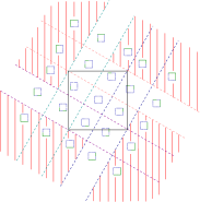
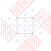
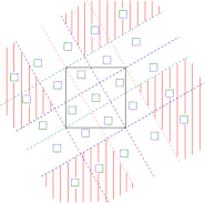
Figure 7: Shape of boundary data with respect to ${\mathbf{x}}_{0}$ (from left to right, cases 1,2,3).

4.2 Numerical results

We perform numerical experiments by considering the following case

$$\Omega=(0,1)^{2}\,,\quad\partial\Omega_{D}=\bigl{(}\{0\}\times\bigl{[}0,\frac{1}{2}\bigr{]}\bigr{)}\cup\bigl{(}\bigl{[}0,1\bigr{]}\times\{0\}\bigr{)}\,,\quad\partial\Omega_{N}=\partial\Omega\setminus\partial\Omega_{D}\,,$$

and using above vector field

$${\mathbf{m}}({\mathbf{x}})=R_{\theta}({\mathbf{x}}-{\mathbf{x}}_{0})\,.$$

We only consider the case of a linear feedback. Let us write down the problem.

$$\left\{\begin{array}[]{l}u^{\prime\prime}-\Delta u=0\\ u=0\\ \partial_{\nu}u=-{\mathbf{m}}.{\boldsymbol{\nu}}\,u^{\prime}\\ u(0)=u_{0}\\ u^{{}^{\prime}}(0)=u_{1}\end{array}\right.\left.\begin{array}[]{l}\text{in }\Omega\times\mathbb{R}_{+}^{\ast}\,,\\ \text{on }\partial\Omega_{D}\times\mathbb{R}_{+}^{\ast}\,,\\ \text{on }\partial\Omega_{N}\times\mathbb{R}_{+}^{\ast}\,,\\ \text{in }\Omega\,,\\ \text{in }\Omega\,.\end{array}\right.$$

We will investigate cases when $\theta$ varies in $[0,\arctan(2)]$. A particular case is given in Figure 8.

Figure 8: When ${\mathbf{x}}_{0}$ belongs to ${\mathcal{D}}_{\theta}$, geometrical condition (6) is satisfied at ${\boldsymbol{\alpha}}$.

Our aim here is to study numerically the variations of the speed of stabilization with respect to the position of ${\mathbf{x}}_{0}$ and the value of $\theta$.
To this end, we have built a finite differences scheme (in space). This leads to a linear second order differential equation

$$U^{\prime\prime}+BU^{\prime}+KU=0\,,$$ (18)

where $B$ is the feedback matrix and $-K$ is the discretized Laplace operator.
Let us define $\,\displaystyle{V=K^{1/2}U}$. Above differential equation can be rewritten as follows

$$\left(\begin{array}[]{l}V\\ U^{\prime}\end{array}\right)^{\prime}=\left(\begin{array}[]{c}0\\ -K^{1/2}\end{array}\begin{array}[]{l}K^{1/2}\\ -B\end{array}\right)\left(\begin{array}[]{l}V\\ U^{\prime}\end{array}\right)$$

and the energy function can be approximated by $\,\displaystyle{\frac{1}{2}(\langle U,KU\rangle+\|U^{\prime}\|^{2})=\frac{1}{2}(\|V\|^{2}+\|U^{\prime}\|^{2})}$.
The decreasing rate is given by the highest eigenvalue of above matrix. Results of our computations are shown in Figure 9 where we built the decreasing rate as a function depending on $\theta$ and the position of ${\mathbf{x}}_{0}$ represented by the abscissa $\lambda$ along ${\mathcal{D}}_{\theta}$.

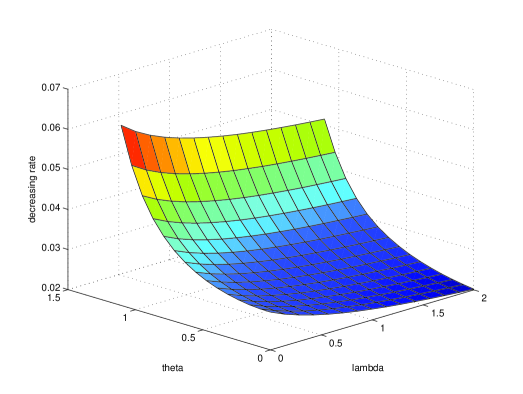
Figure 9: Dependance of the decreasing rate with respect to $\theta$, $\lambda$.

It can be observed that in this case, the decreasing rate is increasing with $\theta$ and the best position for ${\mathbf{x}}_{0}$ is the origin of half-line ${\mathcal{D}}_{\theta}$.

Acknowledgments. This work is partly supported by FONDECYT 1061263 and ECOS-CONICYT CO4E08.

References

- [1] Brézis, H., 1973, Opérateurs maximaux monotones et semi-groupes de contractions dans les espaces de Hilbert, Math. studies 5, North Holland.
- [2] Banasiak, J., Roach, G.-F., 1989, On mixed boundary value problems of Dirichlet oblique-derivative type in plane domains with piecewise differentiable boundary. J. Diff. Equations, 79, no 1, 111-131.
- [3] Bardos, C., Lebeau, G., Rauch, J., 1992, Sharp sufficient conditions for the observation, control and stabilization of waves from the boundary. SIAM J. Control Optim., 30, no 5, 1024-1065.
- [4] Bey, R., Lohéac, J.-P., Moussaoui, M., 1999, Singularities of the solution of a mixed problem for a general second order elliptic equation and boundary stabilization of the wave equation. J. Math. pures et appli., 78, 1043-1067.
- [5] Conrad, F., Rao, B., 1993, Decay of solutions of the wave equation in a star-shaped domain with non linear boundary feedback. Asymptotic Analysis, 7, no 1, 159-177.
- [6] Grisvard, P., 1985, Elliptic problems in nonsmooth domains. Pitman, London.
- [7] Grisvard, P., 1989, Contrôlabilité exacte des solutions de l’équation des ondes en présence de singularités. J. Math. pures et appli., 68, 215-259.
- [8] Kozlov, V. A., Maz’ya, V. G., Rossmann, J., 1997, Elliptic Boundary Value Problems in Domains with Point Singularities, AMS, Providence.
- [9] Komornik, V., 1994, Exact controllability and stabilization; the multiplier method. Masson-John Wiley, Paris.
- [10] Komornik, V., Zuazua, E., 1990, A direct method for the boundary stabilization of the wave equation. J. Math. pures et appl., 69, 33-54.
- [11] Lions, J.-L., 1988, Contrôlabilité exacte, stabilisation et perturbations de systèmes distribués. RMA 8, Masson, Paris.
- [12] Ho, L.F., 1986, Observabilité frontière de l’équation des ondes. C. R. Acad. Sci. Paris, Sér. I Math. 302, 443-446.
- [13] Moussaoui, M., 1996, Singularités des solutions du problème mêlé, contrôlabilité exacte et stabilisation frontière. ESAIM Proceedings, Élasticité, Viscoélasticité et Contrôle optimal, Huitièmes Entretiens du Centre Jacques Cartier, 157-168.
- [14] Nečas, J., 1967, Les méthodes directes en théorie des équations elliptiques. Masson, Paris.
- [15] Osses, A., 1998, Une nouvelle famille de multiplicateurs et applications à la contrôlabilité exacte de l’équation des ondes. C. R. Acad. Sci. Paris, 326, Série I, 1099-1104.
- [16] Osses, A., 2001, A rotated multiplier applied to the controllability of waves, elasticity and tangential Stokes control. SIAM J. Control Optim., 40, no 3, 777-800.
- [17] Rellich F., 1940, Darstellung der Eigenwerte von durch ein Randintegral. Math. Zeitschrift, 46, 635-636.
- [18] Shamir, E., 1968, Regularity of mixed second order elliptic problems. Israel Math. Journal, 6, 150-168.