Results from Droxo. I. The variability of fluorescent Fe 6.4 keV emission in the young star Elias 29

Abstract

Aims. We study the variability of the Fe 6.4 KeV emission line from the Class I young stellar object Elias 29 in the $\rho$ Oph cloud.

Methods. We analysed the data from Elias 29 collected by XMM-Newton during a nine-day, nearly continuous observation of the $\rho$ Oph star-forming region (the Deep Rho-Oph X-ray Observation, named Droxo). The data were subdivided into six homogeneous time intervals, and the six resulting spectra were individually analysed

Results. We detect significant variability in the equivalent width of the Fe 6.4 keV emission line from Elias 29. The 6.4 keV line is absent during the first time interval of observation and appears at its maximum strength during the second time interval (90 ks after Elias 29 undergoes a strong flare). The X-ray thermal emission is unchanged between the two observation segments, while line variability is present at a 99.9% confidence level. Given the significant line variability in the absence of variations in the X-ray ionising continuum and the weakness of the photoionising continuum from the star’s thermal X-ray emission, we suggest that the fluorescence may be induced by collisional ionisation from an (unseen) population of non-thermal electrons. We speculate on the possibility that the electrons are accelerated in a reconnection event of a magnetically confined accretion loop, connecting the young star to its circumstellar disk.

1 Introduction

The X-ray emission from young stellar objects (YSOs) at CCD-resolution is usually modelled as thermal emission from a hot plasma in coronal equilibrium, with higher characteristic temperatures than observed in older and less active stars. An interesting deviation from a pure thermal X-ray spectrum is the presence of fluorescent emission from neutral (or weakly ionised) Fe as shown by the presence of the 6.4 keV line. This was first detected by Imanishi et al. (2001) in the X-ray emission of the YSO YLW16A in $\rho$-Oph, during a large flare: in addition to the Fe xxv complex at 6.7 keV, a 6.4 keV emission line was clearly visibe. Such fluorescence line is produced when energetic X-rays photoionise cold material close to the X-ray source, and it is therefore a useful diagnostic tool of the geometry of the X-ray emitting source and its surroundings.

Since 2001, detections of the Fe K fluorescent emission line at 6.4-keV in the spectra of YSOs have been reported by a number of authors. Tsujimoto et al. (2005) has identified seven sources with an excess emission at 6.4 keV among 127 observations of YSOs within the COUP observation of Orion; Favata et al. (2005b) report 6.4 keV fluorescent emission in Elias 29 in $\rho$-Oph both during quiescent and flaring emission, unlike all other reported detection of Fe fluorescent emission in YSOs that were made during intense flaring; Giardino et al. (2007) have detected Fe 6.4 keV emission from a low-mass young star in Serpens, during an intense, long-duration flare. Recently, Czesla & Schmitt (2007) have reported intense Fe fluorescent emission in the spectrum of V 1486 Ori during a strong flare, when the plasma reached a temperature in excess of 10 keV.

The 6.4 keV fluorescent line has been detected in different classes of X-ray emitters: X-ray binaries, active galactic nuclei (AGNs), massive stars, supernova remnants, and the Sun itself during flares. In the case of the Sun, the fluorescing material is the solar photosphere, in the YSOs, however, indications are that the material in the circumstellar disk and its related accretion structures could be responsible for the fluorescence. The typical equivalent width of the 6.4 keV emission line in the studies mentioned above is of the order of 150 eV and is too large to be explained with fluorescent emission in the stellar photosphere or in diffuse circumstellar material (e.g. Tsujimoto et al., 2005; Favata et al., 2005b). This scenario implies that the disk is “bathed” in high-energy X-rays emitted by the star, with significant astrophysical implications; for instance, X-rays, in addition to cosmic rays, would play an important role in photoionising the circumstellar material around young star and thus in coupling the gas to the ambient magnetic field (as suggested by e.g. Glassgold et al., 2000). Ceccarelli et al. (2002) suggest that the “hot” component they observe in the disk, in the infrared, is heated by the stellar high-energy emission.

Figure 1: The light curve of Elias 29 over the nine days of the Droxo observation from PN (top), MOS1 (bottom-left), and MOS2 (bottom-right). The line with error bars gives the background-subtracted light curve of the source, while the thinner line without error bars gives the total counts (source plus background). The 6 time intervals that we selected for the spectral analysis, on the basis of the PN data, are indicated.

Observations of the time variability of the Fe 6.4 keV emission in YSOs would provide useful constraints on the geometry and sizes of the star-accretion disk system and of other circumstellar structures such as funnel flows, jets, or wind columns. We present here the results of a time-resolved spectral study of the X-ray emission of Elias 29, during $\sim 9$ days of nearly continuous observation by XMM-Newton in the context of the ultra-deep observation of $\rho$-Oph, named Droxo (from Deep Rho-Oph X-ray observation – Pillitteri et al., 2007). We investigated the presence of variations in its strong Fe 6.4 keV emission over the 9-day time scale covered by the observations.

This paper is structured as follows. After a summary, below, of the properties of Elias 29, the observations and data analysis are briefly presented in Sect. 2. Results are summarised in Sect. 3; the simulations carried out to assess the reliability of the line detections and the significance of its variability are described in Sect. 4. The results are discussed in Sect. 5.

1.1 Elias 29 (GY214)

Elias 29 (16:27:09.4, $-$24:37:18.9) with a bolometric luminosity $L=26-27.5\leavevmode\nobreak\ L_{\sun}$ (Bontemps et al., 2001; Natta et al., 2006) is the most luminous Class I YSO in the $\rho$-Oph cloud. Muzerolle et al. (1998) used the luminosity in the Br$\gamma$ line to determine the object’s accretion luminosity at $L_{\rm acc}$ = $15-18L_{\sun}$, which makes it the source with the highest accretion luminosity in their sample. More recently, Natta et al. (2006) used the luminosity of the hydrogen recombination lines to derive an accretion luminosity of 28.8 $L_{\sun}$.

Using millimeter interferometric observations, Boogert et al. (2002) resolved the emission from the disk and the envelope surrounding Elias 29, showing that the disk is in a relatively face-on orientation ($i<60^{\circ}$), which explains many of the remarkable observational features of this source, such as its flat spectral energy distribution, its brightness in the near-infrared, the extended components found in speckle interferometry observations, and its high-velocity molecular outflow. Their best-fitting disk model has an inner radius of 0.01 AU, outer radius of 500 AU, and a mass $M=0.012M_{\sun}$.

Elias 29 was previously observed in X-rays with ASCA, Chandra  and XMM-Newton. In the Chandra observation (Imanishi et al., 2001), the source quiescent phase is characterised by a temperature of 4.3 keV and luminosity of $2.0\times 10^{30}$ erg s^-1, fully consistent with the values derived from the subsequent XMM-Newton observations by Ozawa et al. (2005): $kT=(3.6-5.1)$ keV, $N({\rm H})=(4.4-5.3)\times 10^{22}$ cm^-2, $Z=(0.8-1.3)\leavevmode\nobreak\ Z_{\sun}$, and $L_{\rm X}=2.8\times 10^{30}$ erg s^-1. The source was seen flaring during one of the ASCA observations (Kamata et al., 1997) and during the Chandra observation. The two flares had similar intensity and duration with an $e$-folding time of $\sim 10$ ks (Tsuboi et al., 2000; Imanishi et al., 2001).

2 Observations and data analysis

The Droxo program is a nominal 500 ks observation of the $\rho$-Ophiuchi star-forming region performed by the EPIC camera on board the XMM-Newton satellite. The observation was performed over 9.4 days, starting 8 March 2005 (orbits 0961–0965). Details of the observations and data reduction procedure are given in Pillitteri et al. (2007). The preliminary data reduction was done with SAS software version 6.5 in order to obtain lists of photon events calibrated both in energy and astrometry for the three instruments, MOS1, MOS2, and PN, for each orbit. The data were filtered in the energy band 0.3–10. keV, and only events with pattern $<4$ and flag $=0$ were retained for the spectral analysis. The spectral analysis was performed using the xspec package V11.2, after rebinning the spectra to a minimum of 20 source counts per (variable width) spectral bin.

3 Results

Figure 1 shows the light curve of Elias 29 from the three instruments, PN, MOS1, and MOS2, and the six time intervals that we selected for our spectral analysis. On the basis of the PN data, we selected 5 time intervals with low background (hereafter “seg1” to “seg5”), plus one time interval covering the strong flare at about 94 ks from the beginning of the observation. During “seg1”, the MOS1 camera was very likely hit by a micro-meteorite (which compromised one of the chips) and the instrument was switched off for the rest of this segment of the observation, during the flare and part of “seg2”. MOS2 data are available for all the segments of observation, but are insufficient during the flare, thus, we did not include the “flare” time interval in the joint spectral analysis of PN and MOS data. In addition, we only used PN and MOS2 data for “seg1” and “seg2”.

The spectra were initially modelled by an absorbed one-temperature plasma model. The results of the six spectral fits for the PN data alone are reported in Table 1 and the results of the (five) joint fits to the PN, MOS1, and MOS2 data in Table 2. For each time-interval, the values of the spectral parameters derived from the simultaneous fitting are very similar to the values derived from the PN data alone. The error bars in the best-fit parameters improve marginally, but $\chi^{2}$ values worsen, likely because of calibration uncertainties.

The spectra and the fits for “seg1” and “seg2” are shown in Fig. 2 and the spectrum for the flare in Fig. 3. The average values of the source’s spectral parameters while quiescent ($N({\rm H})=6.8\times 10^{22}$ cm^-2, $kT=3.7$ keV, and $Z=0.8\leavevmode\nobreak\ Z_{\sun}$) are very similar to the values derived from previous observations, so is its quiescent luminosity $L_{\rm X}\sim 10^{30}$ erg s^-1, with no evidence of long-term variability.

The X-ray flare is similar to other events previously observed from this source. During the flare, the source counts first increased impulsively by a factor of $\sim 8$ and then decreased exponentially with a decay time of $\sim 6$ ks. The source spectrum during the flare is shown in Fig. 3, together with the spectral fit. As presented in Table 1, the fitted value of the plasma temperature does not appear to change significantly during the flare, possibly due to the stringent processing criteria applied to the data that resulted in the events of the flare peak being discarded.

From Tables 1 and 2, it is apparent that the best-fit values of $N({\rm H})$, $kT$, and $Z$ for the different time intervals do not show significant variations, since they are all consistent with each other within $2\sigma$. This is also apparent by comparing the PN and MOS2 spectra from “seg1” and “seg2” in Fig. 2, where the overall spectral shape and amplitude are very similar during the two time intervals (in both instruments). On closer inspection, however, a significant difference between the two time intervals becomes apparent: during time interval “seg2”, a visible excess of emission around 6.4 keV, the energy of the Fe fluorescent line, is present both in the PN and MOS2 data.

To quantify this excess and monitor its variation, we repeated the spectral fits of the spectra with an absorbed 1T plasma model and an additional Gaussian line component at 6.4 keV. The position and width (10 eV) of this component were constrained during the fit, while its normalisation was left free to vary. The other parameters of the absorbed 1T plasma model (absorbing column density, temperature, and normalisation of the thermal spectrum) were also free parameters in the fit. The spectra and spectral fits to the six PN spectra in the energy range $\Delta E=4-8$ keV are shown in Fig. 4. The strong excess emission at 6.4 keV in the spectra of “seg2” is well accounted for by the fitted line, while it is clear that no such additional line at 6.4 keV is needed to fit the data from “seg1”. The four other spectra are somewhat in between these two extremes in regard to an excess of emission at 6.4 keV.

The results from the spectral fits to the PN data with the additional line at 6.4 keV are summarised in Table 3. As can be seen by comparing Tables 1 and 3, the fitted values for absorbing column density, temperature, metallicity, and normalisation of the thermal spectrum are not affected by the addition of the 6.4 keV-line component. The null-hypothesis probability of all the fits improves, except for “seg1”, for which the null-hypothesis probability decreases marginally. Indeed, an excess of emission at 6.4 keV does not appear to be present at all in this spectrum, so that there is no reason to add an extra line component at 6.4 keV. We have also added this component to the spectral fit of “seg1” to make the fits homogeneous and directly comparable. The equivalent width of the fitted line appears to vary significantly from the 13 eV of “seg1” (where the excess emission at 6.4 keV does not seem to be present) to the 249 eV of “seg2”.

Table 4 summarises the results of the simultaneous spectral fitting of PN and MOS data with an absorbed 1T plasma model and an additional Gaussian line component at 6.4 keV: the results obtained from this joint spectral analysis are again fully consistent with the results from the PN data alone (compare Table 3 and 4). The strong variation in the intensity of the excess emission at 6.4 keV between “seg1” and “seg2” is confirmed; the best-fit line equivalent width varies from 10 eV in “seg1” (where the line also appears to be absent in the MOS2 data) to 194 eV in “seg2” (where the excess of emission is also strong in the MOS2 data – see Fig. 2). For “seg3” and “seg4”, the equivalent width of the emission at 6.4 keV derived from the joint fits differs by $\sim$50% from the value derived from the PN data alone, but best-fit values of the line’s flux are consistent within the two data-sets; for “seg5”, the equivalent width of the emission at 6.4 keV derived from the two spectral analysis are very similar.

As described in Sect. 4, we have performed a set of Monte Carlo simulations of the PN spectra to assess whether the line at 6.4 keV seen in the spectra from “seg2” to “seg5” is real rather than the result of statistical fluctuations in the data. The results of these simulations are summarised in the last column of Table 3, which gives the probability that a line at 6.4 keV, with equivalent width equal to, or greater than, the best-fit value, could be the result of random fluctuations for each segment. This probability is high for “seg1” and the “flare” segment, for which the data are consistent with the absence of a line in the spectrum. Conversely, the probability that the excess of emission in “seg2” and “seg5” is due to noise fluctuations is low (0.1% and 0.2%, respectively). For time intervals “seg3” and “seg4” the situation is less clear, since with a probability of 4.2% and 3.5%, respectively, that the excess at 6.4 keV could be due to random fluctuations, the evidence for intrinsic emission is less compelling. Nevertheless an analysis of the spectrum of the source integrated over the time intervals “seg3”, “seg4”, and “seg5” shows that the evidence for the presence of the line is very strong, with a probability that the excess at 6.4 keV is due to random fluctuation of less than one in a thousand (as summarised in the last line of Table 3).

Figure 2: Elias 29 spectra from PN (top) and MOS2 (bottom) with spectral fits, during “seg1” (before the flare, left) and “seg2” (after the flare, right). The spectra (from the two time intervals) are very similar in overall shape and amplitude, and the fits (with an absorbed 1T plasma model) result in very similar parameters. During “seg2”, however, a significant excess of emission at 6.4 keV is present, which is not visible in the data from “seg1”. All the spectra are rebinned to a minimum of 20 source counts per (variable width) spectral bin.

Figure 3: The spectrum of Elias 29 (PN data) during the strong flare between “seg1” and “seg2”, together with the best-fit one-temperature model.

The simulations described in Sect. 4 also show that the variation in the line’s equivalent width seen between “seg1” (where the line appear to be absent or extremely weak) and “seg2” are very likely intrinsic (with a probability of 99.9%).

Table 1: Best-fit parameters from the fits to the spectra of Elias 29, during 6 different time intervals (PN data only), using an absorbed 1T thermal model. Reduced $\chi^{2}$ and null-hypothesis probability ($P$) for the fits are also given.

Time interval	$N({\rm H})$	$kT$	$Z$	$E\!M$	$\chi^{2}$/d.o.f.	$P$	$F_{\rm X}$
	$N_{22}$	keV	$Z_{\odot}$	$E\!M_{53}$			$F_{-13}$
seg1	5.7 $\pm$ 0.7	4.6 $\pm$ 0.9	1.0 $\pm$ 0.3	1.4 $\pm$ 0.5	1.0	0.6	1.8
flare	9.5 $\pm$ 2.0	4.1 $\pm$ 1.5	0.9 $\pm$ 0.3	8.3 $\pm$ 6.3	0.9	0.5	7.5
seg2	8.1 $\pm$ 1.3	3.1 $\pm$ 0.8	1.0 $\pm$ 0.3	1.4 $\pm$ 0.9	1.5	0.0	1.1
seg3	6.6 $\pm$ 0.8	3.4 $\pm$ 0.7	0.7 $\pm$ 0.2	1.5 $\pm$ 0.8	1.0	0.5	1.3
seg4	7.7 $\pm$ 0.6	3.7 $\pm$ 0.5	0.7 $\pm$ 0.1	3.1 $\pm$ 0.9	1.4	0.0	2.7
seg5	4.9 $\pm$ 0.4	4.7 $\pm$ 0.8	0.6 $\pm$ 0.1	2.0 $\pm$ 0.6	1.3	0.1	2.5

Units are $N_{22}=10^{22}\leavevmode\nobreak\ {\rm cm^{-2}}$, $E\!M_{53}=10^{53}$ cm^-3, and $F_{-13}=10^{-13}$ erg cm^-2 s^-1. The spectral fits were carried out in the energy range 1.0–9.0 keV. Flux values refer to energy range 1.0-7.5 keV. The error bars are at 1$\sigma$.

Table 2: Best-fit parameters from the joint fits to PN, MOS1 and, MOS2 spectra of Elias 29, during 5 different time intervals, using an absorbed 1T thermal model.

Time interval	$N({\rm H})$	$kT$	$Z$	$E\!M$	$\chi^{2}$/d.o.f.	$P$	$F_{\rm X}$
	$N_{22}$	keV	$Z_{\odot}$	$E\!M_{53}$			$F_{-13}$
seg1†	5.5 $\pm$ 0.5	4.4 $\pm$ 0.7	1.0 $\pm$ 0.2	1.7 $\pm$ 0.5	1.1	0.1	2.1
seg2†	7.4 $\pm$ 0.8	3.8 $\pm$ 0.7	0.8 $\pm$ 0.2	1.5 $\pm$ 0.6	1.6	0.0	1.3
seg3	6.6 $\pm$ 0.5	3.5 $\pm$ 0.5	0.7 $\pm$ 0.1	2.0 $\pm$ 0.5	1.1	0.2	1.7
seg4	7.5 $\pm$ 0.4	3.7 $\pm$ 0.4	0.7 $\pm$ 0.1	3.5 $\pm$ 0.8	1.5	0.0	3.0
seg5	5.7 $\pm$ 0.4	4.0 $\pm$ 0.5	0.5 $\pm$ 0.1	2.8 $\pm$ 0.7	1.6	0.0	2.3

†MOS1 data (mostly) unavailable for this time interval so only PN and MOS2 data were used.

Table 3: Best-fit parameters from the fits to the spectra of Elias 29, during 6 different time intervals (PN data only), using an absorbed 1T thermal model with an additional line at 6.4 keV (Fe fluorescent line). For the line, the total flux in the line ($f_{\rm 6.4keV}$ in units of $f_{-6}=10^{-6}$ photons cm^-2 s^-1) and the equivalent width ($W_{\rm 6.4\leavevmode\nobreak\ keV}$) are given.

Time interval	$N({\rm H})$	$kT$	$Z$	$E\!M$	$f_{\rm 6.4keV}$	$W_{\rm 6.4\leavevmode\nobreak\ keV}$	$\chi^{2}$/d.o.f.	$P$	$F_{\rm X}$	$R_{\rm 6.4keV}$‡
	$N_{22}$	keV	$Z_{\odot}$	$E\!M_{53}$	$f_{-6}$	eV			$F_{-13}$	%
seg1	5.5 $\pm$ 0.7	4.8 $\pm$ 1.0	1.1 $\pm$ 0.3	1.3 $\pm$ 0.5	0.1 $\pm$ 0.7	13.0	1.0	0.5	1.8	45
flare	9.4 $\pm$ 2.0	3.9 $\pm$ 1.4	0.9 $\pm$ 0.3	8.3 $\pm$ 6.2	2.0 $\pm$ 5.9	60.2	0.9	0.6	7.5	23
seg2	8.2 $\pm$ 1.3	2.8 $\pm$ 0.6	1.1 $\pm$ 0.3	1.4 $\pm$ 0.8	1.1 $\pm$ 0.6	249.0	1.3	0.1	1.1	0.1
seg3	6.6 $\pm$ 0.8	3.3 $\pm$ 0.6	0.7 $\pm$ 0.2	1.6 $\pm$ 0.8	0.5 $\pm$ 0.5	108.0	0.9	0.6	1.3	4.2
seg4	7.6 $\pm$ 0.6	3.6 $\pm$ 0.4	0.7 $\pm$ 0.1	3.2 $\pm$ 0.9	0.7 $\pm$ 0.7	67.8	1.3	0.1	2.7	3.5
seg5	4.9 $\pm$ 0.4	4.5 $\pm$ 0.8	0.6 $\pm$ 0.1	2.1 $\pm$ 0.6	1.1 $\pm$ 0.8	162.0	1.2	0.2	2.5	0.2
seg3$+$seg4$+$seg5$\diamondsuit$	6.4 $\pm$ 0.3	3.9 $\pm$ 0.3	0.6 $\pm$ 0.1	2.2 $\pm$ 0.4	1.0 $\pm$ 0.3	147.0	1.3	0.0	2.1	0.0

‡Probability that a line with a best-fit value equal or greater than $W_{\rm 6.4\leavevmode\nobreak\ keV}$ could be due to a random fluctuation in the data, as estimated via Monte Carlo simulations (see Sect. 3 and 4).

$\diamondsuit$ Results for the fit to the source’s spectrum integrated over time intervals “seg3”, “seg4”, and “seg5”

Table 4: Best-fit parameters from joint fits to PN, MOS1 and MOS2 spectra of Elias 29, during 5 different time intervals, using an absorbed 1T thermal model with an additional line at 6.4 keV (Fe fluorescent line).

Time interval	$N({\rm H})$	$kT$	$Z$	$E\!M$	$f_{\rm 6.4keV}$	$W_{\rm 6.4\leavevmode\nobreak\ keV}$	$\chi^{2}$/d.o.f.	$P$	$F_{\rm X}$
	$N_{22}$	keV	$Z_{\odot}$	$E\!M_{53}$	$f_{-6}$	eV			$F_{-13}$
seg1†	5.5 $\pm$ 0.5	4.3 $\pm$ 0.8	1.0 $\pm$ 0.2	1.7 $\pm$ 0.5	0.1 $\pm$ 0.7	9.7	1.2	0.1	2.1
seg2†	7.5 $\pm$ 0.8	3.5 $\pm$ 0.7	0.9 $\pm$ 0.2	1.6 $\pm$ 0.6	1.1 $\pm$ 0.7	194.0	1.4	0.0	1.3
seg3	6.7 $\pm$ 0.6	3.3 $\pm$ 0.5	0.7 $\pm$ 0.2	2.1 $\pm$ 0.7	0.4 $\pm$ 0.6	68.7	1.1	0.3	1.7
seg4	7.5 $\pm$ 0.4	3.5 $\pm$ 0.3	0.7 $\pm$ 0.1	3.6 $\pm$ 0.8	1.2 $\pm$ 0.7	118.0	1.4	0.0	3.0
seg5	5.8 $\pm$ 0.4	3.7 $\pm$ 0.5	0.5 $\pm$ 0.1	2.9 $\pm$ 0.8	1.2 $\pm$ 0.7	152.0	1.5	0.0	2.3

†MOS1 data (mostly) unavailable for this time interval so only PN and MOS2 data were used.

Figure 4: Spectra (PN) and spectral fits of Elias 29 during 6 different time intervals, between 4 and 8 keV. From left to right, top to bottom, spectra are from time intervals “seg1”, “flare”, “seg2”, “seg3”, “seg4”, and “seg5” (these intervals are indicated in Fig. 1). Fits were performed using an absorbed 1T thermal model with the addition of a line at 6.4 keV (indicated in the plots by a dash-dotted line). Note the strong excess of emission at 6.4 keV in the spectra for “seg2”, which does not appear to be present in the spectrum from the first time interval.

Figure 5: The spectrum (PN data) of Elias 29, between 4 and 8 keV, integrated over the four time intervals of quiescent emission where an excess at 6.4 keV appears to be present. With the improved statistic of this long time span, the presence of 6.4 keV Fe fluorescent emission is very clear.

To further constrain the properties of the Fe 6.4 keV emission from Elias 29, we derived the spectrum of the source integrated over the quiescent time intervals where the excess at 6.4 keV appears to be present (although with varying significance), i.e. intervals “seg2”, “seg3”, “seg4”, and “seg5” (PN data only). The summed spectrum between 4 and 8 keV is shown in Fig. 5, where the emission line at 6.4 keV is very clear thanks to the the improved statistic. A fit with an absorbed 1T model to this spectrum yields $N({\rm H})=6.7\times 10^{22}$ cm^-2, $kT=3.7$ keV and $Z=0.7\leavevmode\nobreak\ Z_{\sun}$ with a null hypothesis probability $P=3.5\times 10^{-5}$. The spectral parameters are very similar to the average values derived above from the fits to the individual five quiescent time intervals, although the fit probability is rather low. With the addition of a line at 6.4 keV, the fit probability increases substantially to $P=2.1\times 10^{-3}$ (and the values of the parameters of the 1T model hardly change). In this case we left the position of the Gaussian line free to vary during the fit, together with its normalisation. The fitted line equivalent width is $W_{\rm 6.4\leavevmode\nobreak\ keV}=143$ eV and its position is $6.44\pm 0.03$, fully consistent with being Fe K fluorescent emission. Indeed, although the reliability is limited (the quoted error is at 1$\sigma$), the line peak energy of 6.44 keV would suggest that the fluorescing Fe is Neon-like: Fe xvii or so. The Fe K fluorescent emission line energy is, in fact, a slowly increasing function of ionisation state, rising from 6.40 keV in Fe i to 6.45 keV in Fe xvii (House, 1969; George & Fabian, 1991).

4 Simulations

Figure 6: Distributions of the best-fit equivalent width of the 6.4 keV line in two sets of simulations of the spectra of “seg1”. In the top panel the input model to the simulation did not contain a Gaussian line component at 6.4 keV, so the distribution gives the probability of deriving a spurious emission line with a given equivalent width. The best-fit equivalent width derived for “seg1” of 13 eV is consistent with the line being spurious. In the bottom panel the input model contained a Gaussian line component at 6.4 keV with $W_{\rm 6.4\leavevmode\nobreak\ keV}=249$ eV, as derived in the data for “seg2”. In this case, the probability of detecting a Gaussian component with $W_{\rm 6.4\leavevmode\nobreak\ keV}\leq 13$ eV is very low (0.1%). Each simulation consisted of 1000 random realisations of the input model.

To quantify the reliability of the detection of the 6.4 keV emission in the different spectra of Elias 29, we performed a set of Monte Carlo simulations of the PN spectra. For each time interval discussed in Sect. 3, 1000 random realisations of the absorbed 1T-model fitted to the spectrum without the additional Gaussian component at 6.4 keV (as per Table 1) were generated using xspec. These random realisations have the same noise characteristics of the data and the same energy binning of the real data (for which channels are combined to a minimum of 20 counts per energy bin). The 1000 simulated spectra were then fitted with the same procedure used for the real data. First a fit with an absorbed 1T plasma model was performed then a Gaussian line component at 6.4 keV with a narrow $\sigma$ of 10 eV was added to the model and the simulated data were re-fitted. The line position and width were kept fixed during this fit, while its normalisation was left unconstrained. The equivalent width of the fitted line was then computed for all 1000 fits for each time interval.

Since the input model to the simulated spectra did not contain any emission line at 6.4 keV, the number (over 1000) of fitted spectra with a fitted line with a given $W_{\rm 6.4\leavevmode\nobreak\ keV}$ gives the probability that a line with that equivalent width could be measured in the real spectrum because of the noise’s random fluctuations. For example, in the case of “seg1” the number of simulated spectra with $W_{\rm 6.4\leavevmode\nobreak\ keV}\geq 13$ eV ($W_{\rm 6.4\leavevmode\nobreak\ keV}=13$ eV being the best-fit equivalent width in the real data) is 453, thus, the probability of deriving a spurious line with $W_{\rm 6.4\leavevmode\nobreak\ keV}\geq 13$ eV from the spectrum of “seg1” is 45%. This can be seen by looking at the top panel of Fig. 6, which gives the distribution of $W_{\rm 6.4\leavevmode\nobreak\ keV}$ for the fitted lines for the simulation of “seg1”. Note that, in the case of “seg1”, there is no visible excess of emission at 6.4 keV, so a high incidence of simulated spectra with $W_{\rm 6.4\leavevmode\nobreak\ keV}\geq 13$ eV is consistent with the absence of the line in the intrinsic spectrum.

In the case of “seg2”, on the other hand, the number of simulated spectra with $W_{\rm 6.4\leavevmode\nobreak\ keV}\geq 249$ eV is 1 (over 1000 simulations), indicating that the excess at 6.4 keV seen in the spectrum of “seg2” is very likely intrinsic to the source. The results of all these simulations for all the different time intervals, in terms of the probability of by chance observing a line with a value of $W_{\rm 6.4\leavevmode\nobreak\ keV}$ greater or equal to the one measured in the data, are summarised in Table 3. For illustration, the distribution of the fitted spectral parameters $N({\rm H})$, $kT$, and $Z$ for the 1000 simulations for “seg1” are given in Fig. 7.

Finally, to assess the probability that a line with the same equivalent width as derived in “seg2” ($W_{\rm 6.4\leavevmode\nobreak\ keV}=249$ eV) could be present in the source’s intrinsic spectrum of “seg1”, but could go undetected due to the noise fluctuation, we performed one additional simulation for “seg1”. In this case, the simulation input model was the best-fit absorbed 1T model for “seg1” (as per Table 1) with the addition of a Gaussian line at 6.4 keV with $W_{\rm 6.4\leavevmode\nobreak\ keV}=249$ eV. In this case, the number of simulated spectra for which we derived a fitted line at 6.4 keV with $W_{\rm 6.4\leavevmode\nobreak\ keV}\leq 13$ eV is 1 (over 1000), as can be seen from Fig. 6. In other words, the probability that during “seg1” an intrinsic emission line with the same $W_{\rm 6.4\leavevmode\nobreak\ keV}$ as derived in “seg2” could result in an observed excess with $W_{\rm 6.4\leavevmode\nobreak\ keV}\leq 13$ is 0.1%. This indicates that the strong variations in Fe 6.4 keV emission detected in the data between “seg1” and “seg2” are very likely intrinsic.

Figure 7: Distributions of the best-fit values of the absorbing column density, plasma temperature, and metallicity in the the simulations of the spectra of “seg1”. The vertical dashed lines give the parameter values used in the simulation’s input model. The simulation consisted in 1000 random realisations of the spectral model fitted to the data of “seg1”.

5 Discussion

As mentioned in the introduction, previous works have considered that the most likely location of the cold material traced by fluorescent emission is, in YSOs, the circumstellar disk, as no fluorescence, whether from the photosphere or from a circumstellar shell, can result in the large equivalent widths observed (approximately 150 eV), given a plausible thermal photoionising continuum.

The radiative transfer computation necessary for determining the fluorescent equivalent width in the case of an optically thick target (i.e. a stellar photosphere) shows that, in the case of a semi-isotropically illuminated slab (such as a photosphere), the equivalent width $W_{\rm 6.4\leavevmode\nobreak\ keV}$ varies approximately from 150 to 90 eV (assuming photospheric solar iron abundance), for a power-law incident spectrum with spectral index $\Gamma=1.2$ to 2.1 (George & Fabian, 1991). Given that the thermal spectrum of stellar sources is generally steeper than a power-law spectrum with $\Gamma\sim 2.0$ (e.g. Favata et al., 2005b; Giardino et al., 2007), photospheric emission can hardly explain the observed equivalent widths.

George & Fabian (1991) show that higher equivalent widths for the fluorescent Fe K line can be obtained if the cold material is distributed in a centrally illuminated disk. In this case, for favourable disk inclination angles (near face-on, $i=0^{\circ}-30^{\circ}$), $W_{\rm 6.4\leavevmode\nobreak\ keV}$ varies approximately between 120 and 200 eV for an incident spectrum spectral index $\Gamma=2.3$ to 1.3. This interpretation of the origin of the fluorescent Fe K emission was also proposed by Favata et al. (2005b) for Elias 29, whose accretion disk was shown to be in a relatively face-on orientation ($i<60^{\circ}$) by Boogert et al. (2002). This interpretation cannot, however, easily explain the current set of data.

The remarkable feature of the present data is that the strong Fe 6.4 keV emission, apparent in the second segment of the observation, is absent (or significantly weaker) during the first segment of the observation, while the observed thermal continuum X-ray spectrum is basically unchanged. Although a stellar flare takes places between the two intervals, the radiative lifetimes of fluorescent Fe transitions are negligible compared to the time between the flare and the second observation segment (91 ks) – see e.g. Langhans et al. (1995) for the radiative lifetimes of Fe i and Schnabel et al. (2004) for Fe ii – and therefore the flare cannot explain the 6.4 keV emission observed in the second segment of the observation. To explain the observation, a sustained mechanism ionising the neutral Fe atoms must operate during the rest of the observation, on time scale of days, independent of (and not correlated with) the thermal X-ray emission. This mechanism must be absent during the first segment. This is unlikely to be the stellar X-ray continuum emission, as this emission appears to be unchanged between the first and the second observation segments.

A scenario in which a localised region of photoionised Fe 6.4 keV emission is somehow eclipsed during “seg1” is also difficult to reconcile with the data, given the high equivalent width of the line ($W_{\rm 6.4\leavevmode\nobreak\ keV}\ga 150$ eV), when this is present. As mentioned above, to explain such a large equivalent width by photoionisation, the favorable geometry of a nearly face-on, centrally illuminated disk is needed in order to maximise the number of atoms whose line emission is free to escape. Requiring that the Fe 6.4 keV emitting region is localised (and in order to be eclipsed by the star in a nearly face-on disk this volume needs to be significantly localised), automatically reduces the equivalent widths that can be obtained. The same line of reasoning applies to a region of localised emission on the stellar photosphere, even more so, given that for the same incident spectrum one obtains smaller line equivalent widths.

The large Fe 6.4 keV equivalent width derived in the second segment, 190 – 250 eV, is also difficult to reconcile with emission from photoionisation of the material in the circumstellar disk. The model of George & Fabian (1991) for a centrally illuminated face-on disk and an incident X-ray spectrum with a power law index of $\Gamma=2.3$, which is appropriate for Elias 29, predicts a maximum equivalent width of only 120 eV, that is, 70 – 130 eV less than the observed best-fit value in segment 2. In addition, the maximum equivalent width of the 6.4 keV line corresponds to the lowest temperature in the thermal spectrum, in contradiction with the expectations from a photoionisation process.

An alternative explanation for the production of the Fe 6.4 keV emission line in solar flares is collisional ionisation of K-shell electrons by a beam of non-thermal electrons (Emslie et al., 1986). This mechanism may also operate in some stellar systems. Osten et al. (2007) have recently observed a superflare on the active binary system II Peg with the Swift telescope. Analysis of the X-ray spectrum from 0.8 to 200 keV from the XRT and BAT instruments reveals evidence of a thermal component with $kT$ in excess of 7 keV, Fe 6.4 keV emission, and a tail of emission out to 200 keV, which can be fit with a power-law model with spectral index $\Gamma\sim 2$. They attribute this power-law hard X-ray emission to non-thermal thick-target bremsstrahlung emission from a population of accelerated electrons and find that collisional ionisation (of photospheric material) from the same non-thermal electrons is a more likely explanation for the 6.4 keV feature than the photoionisation mechanism.

In our case, a superflare is not taking place; indeed, no stellar flare is taking place during the second segment of observation. In a magnetospheric accretion scenario, however, ionised material is magnetically channeled in accretion streams that connect the star to the circumstellar accretion disk (e.g. Calvet & Hartmann, 1992). The observation of very intense long-duration flares in YSOs, which implies flaring loop lengths of tens of stellar radii (Favata et al., 2005a), provides evidence of flaring associated to these accretion streams.

A magnetic reconnection event leading to the acceleration of electrons within one of these structures, connecting the star to the disk, may or may not result in a (soft) X-ray flare event depending on the density of the material confined in the structure itself. If the density of material within the magnetic flux tube is not very high (with column densities from the acceleration site to the photosphere or to the disk of $N\la 10^{20}$ cm^-2), the accelerated particles will impact the stellar photosphere and heat and “evaporate” the chromospheric plasma, providing the hot material that emits the X-ray flare observed between 0.1 and 10 keV. Indeed, the flares for which long flaring loops were derived in Favata et al. (2005a) appear to take place in CTTs with no significant ongoing accretion (hence their “accretion” tubes are not mass-loaded).

In YSOs, which are still strongly accreting, the density of material confined in the accretion tubes is expected to be high. For a fiducial case of mass accretion rate of $10^{-7}M_{\odot}$ yr^-1, Muzerolle et al. (2001) estimate densities of $n_{\rm H}=10^{12}-10^{13}$ cm^-3 at $\sim 2{\rm R_{*}}$, that is, column densities of the order of $N\sim 10^{23}-10^{24}$ cm^-2 assuming a stellar radius of 10¹¹ cm^-2. In Elias 29 with an accretion luminosity of 28.8 $L_{\sun}$, the accretion rate is estimated to be one order of magnitude higher (Natta et al., 2006), so the column density within the accretion tubes will be correspondingly higher. With such a high density, the accelareted electrons produced by a reconnection event in the accretion tube cannot reach the stellar photosphere, but will be decelerated in situ, producing non-thermal (hard) X-ray emission and collisional ionisation of elements such as Fe, which will be largely neutral at a typical temperature of $\sim 7000$ K (Muzerolle et al., 2001). A sketch of the Elias 29 star-disk system with the hypothesised accretion tube where the electron acceleration is taking place is shown in Fig. 8.

To explain the observed long-lasting fluorescent emission, the electron acceleration mechanism should be sustained over several days. While we have no detailed physical mechanism to propose for this, we note that many of the long-lasting flares observed in YSOs by Favata et al. (2005a) require sustained heating of the flaring material to explain the observed duration of the events, which in some cases lasted a few days. The thermodynamic cooling time of the flaring plasma would be much shorter; therefore, to explain the observed long flaring events in YSOs, magnetic reconnection must be ongoing, on time scales of days, similar to what is observed for the Fe 6.4 keV fluorescent emission from Elias 29. The same electron acceleration mechanism could therefore result in long-lasting flares, if it takes place in systems with little ongoing accretion, or in strong Fe 6.4 keV emission, if it takes place in systems with strong ongoing accretion.

In their study, Emslie et al. (1986) provide a relation (Fig. 1 in their paper) between the flux emitted in the 6.4 keV line in the case of electron ionisation, as a function of the column density of material between the electrons’ injection point and the “cold” Fe (where Fe 6.4 keV emission can take place). This column density is zero in our case, since, as mentioned above, the material in the accretion tubes is mostly neutral at temperatures of $\sim 7000$ K. In the diagram, different curves are given for different values of the spectral index, $\Gamma$, of the non-thermal X-ray emission, and the line flux is normalised to an amplitude of non-thermal (power-law) emission of $a=1$ photons cm^-2 s^-1 keV^-1 (at 1 keV).

The flux observed for Elias 29 in the Fe 6.4 keV emission line in the integrated spectrum is $\sim 10^{-6}$ photons cm^-2 s^-1, and from the plot by Emslie et al., 1986 one can see that such a flux can be obtained for a very wide choice of parameter combinations, with $\Gamma$ ranging from 2.1 to 5.0, for $a=10^{-4}-1$ photons cm^-2 s^-1 keV^-1. The parameters $\Gamma$ and $a$ refer to the hard X-ray emission, typically at $E\ga 20$ keV. As discussed by Holman (2003), however, the X-ray spectrum of the non-thermal X-ray emission flattens below the low-energy cutoff ($E_{c}$) of the suprathermal electron responsible for the emission. For example, the bremsstrahlung emission from a beam of electrons, with a power-law spectrum with spectral index $\delta=3$ and low-energy cutoff $E_{c}=50$ keV, has a spectral index of $\Gamma\sim 2$ at $E>E_{c}$, but flattens to $\Gamma\sim 1.3$ between 1 and 10 keV.

For the electron beam model in solar flares, electrons are assumed to have energy higher than 20 keV (e.g. Brown et al., 1990) and recent RHESSI data indicates a low-energy cutoff that is typically $E_{c}=20-40$ keV and can be as high 70 keV (Holman et al., 2003). Using the BREMTHICK code by G. D. Holman, we verified that a non thermal hard X-ray emission with $a=10^{-4}-1$ photons cm^-2 s^-1 keV^-1 and $\Gamma=2-5$, from a population of electrons with $E_{c}\ga 40$ keV, between 1 and 10 keV, would be buried in the star’s thermal emission and thus cannot be constrained without hard-X ray observations. Note, also, that a value of $a=10^{-4}-1$ photons cm^-2 s^-1 keV^-1 would not require an unusually high power input in accelerated electrons.

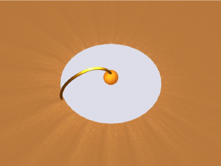
Figure 8: A cartoon of Elias 29 star-disk system with an accretion tube (hypothetical). A magnetic reconnection event within the accretion tube would generate accelerated electrons that could ionise the material and induce Fe K$\alpha$ emission from the accreting material within the tube itself. The system is assumed at a viewing inclination angle $i=30^{\circ}$ ($i=0^{\circ}$ being face-on).

If our proposed mechanism of in situ electron bombardment of neutral or nearly-neutral material is correct, our observations provide additional evidence of strong non-thermal phenomena in young stars and, in particular, of particle bombardment of neutral material in the protoplanetary disk of the young star. In the solar system, such evidence is, for example, provided by the meteorites known as chondrites. Chondrites have a number of peculiar features, as they contain granules (the chondrules) that have been flash heated (on time scales of less than one hour) to some 2000 K, embedded in a rocky matrix with no evidence of heating. Also, the chondrules show evidence of having cooled in a relatively intense magnetic field (of the order of 10 G). Finally, they contain material with peculiar isotopic ratios, with significant amounts of short-lived radio nuclides (e.g. ⁴¹Ca, with a half life of only 0.1 Myr, or ¹⁰Be, with a half life of 1.5 Myr), which therefore cannot be originating in SN nucleosynthesis but must instead be originating in situ (as discussed in detail by e.g. Gounelle et al., 2006). While the observed isotopic anomalies likely require proton (rather than electron) bombardment, our observations provide evidence of in situ acceleration mechanisms closely associated with neutral material from the star’s circumstellar disk, that is, an environment where accelerated non-thermal particles interact with the protoplanetary material from which the meteorites will later grow.

6 Conclusions

So far, the Fe 6.4 keV emission in YSOs has been explained in terms of fluorescent emission from the photoionised (colder) material in the circumstellar disk. This scenario, however, cannot easily explain the observed variability of the Fe 6.4 keV emission in Elias 29, which occurs in the absence of signficant variations of the observed X-ray continuum. The equivalent width of the line at its maximum strength of $\sim 250$ eV is also not easily reconciled with a photoionisation scenario. An alternative line-formation mechanism is collisional excitation by a population of non-thermal electrons. We suggest that these electrons could be accelerated by magnetic reconnection events in the accretion tubes that connect the star to its circumstellar disk. The electrons are decelerated in situ by the accreting material, ionising it and causing the observed Fe 6.4 keV emission.