On the anomalous dimensions of the multiple pomeron exchanges

Abstract

High energy hard scattering in large $N_{c}$ limit can be described by the QCD dipole model. In this paper, single, double and triple BFKL pomeron exchange amplitudes are computed explicitly within the dipole model. Based on the calculation, the general formula $\gamma^{(k)*}_{0}=\chi^{-1}\left(k\chi\left(\frac{1}{2}\right)\right)$ which governs the anomalous dimension of $1\Rightarrow k$ amplitude is conjectured. As far as the unitarity problem is concerned, we find that the anomalous dimension $\gamma$ varies from graph to graph due to the DGLAP evolution. In the end, a comparison between this computation and reggeon field theory is provided.

I Introduction

High energy QCD small-x evolution of hadron can be described by the Balitsky-Fadin-Kuraev-Lipatov (BFKL) PomeronBalitsky:1978ic ; Kuraev:1977fs ; Lipatov:1985uk . BFKL pomeron should be relevant for describing the exponential growth of scattering amplitudes with respect to rapidity. More than a decade ago, the dipole picture of pomeron was discovered by Mueller et alMueller:1993rr ; Mueller:1994jq ; Mueller:1994gb , and the exact equivalenceNavelet:1997tx between the color dipole model and the BFKL pomeron result was verified several years later. Onium-onium scattering at high energy is used to describe this dipole picture of high energy hard scattering in large $N_{c}$ limit. Supposing that $M$, the mass of the onium, is large enough to justify the fixed coupling calculation, one can find that the onium-onium scattering cross section at single pomeron exchange level behaves as

$$\sigma\sim xx^{\prime}\alpha^{2}\exp\left[\left(\alpha_{P}-1\right)Y\right]$$ (1)

where $x$, $x^{\prime}$ are the sizes of the interacting onia, $Y=\ln\frac{s}{M^{2}}$ and $\alpha_{P}-1=\frac{8\alpha C_{F}\ln 2}{\pi}$ with $C_{F}=\frac{N_{c}^{2}-1}{2N_{c}}\Rightarrow\frac{N_{c}}{2}$ in large $N_{c}$ limit. Besides the exponential growth of the cross section, one also gets the anomalous dimension $\gamma=\frac{1}{2}$ as a result of $\sigma$ being proportional to $xx^{\prime}$.(The shift of the exponents of $x^{2}$ and $x^{\prime 2}$ from $1$ is called the anomalous dimension of the BFKL pomeron.)

On the other hand, single pomeron exchange amplitude violates the unitarity and the Froissart bound at extremely high energy. Multiple exchanges of pomerons (here we mean pomeron loops) should be able to reduce the growth rate of the amplitudes, and eventually unitarize it at high energy. Within the dipole model, Kovchegov equationKovchegov:1999yj , a nonlinear evolution equation, is derived by re-summing the fan diagrams(i.e., multiple pomeron exchanges in dipole-nucleus scattering). Recently, there has been a lot of developmentMueller:2004se ; Iancu:2004es ; Munier:2003vc ; Iancu:2004iy ; Mueller:2005ut ; Iancu:2005nj ; Kovner:2005nq ; Hatta:2005rn in high-energy QCD evolution. Evolution equations which include pomeron loops are derivedKovner:2005en+X ; Blaizot:2005vf+X ; Marquet:2005hu ; Levin:2005au ; Enberg:2005cb ; Soyez:2005ha and utilized to QCD phenomenology(e.g., see Hatta:2006hs ; Iancu:2006uc ; Kozlov:2006qw ; Kozlov:2007wm .). As far as the unitarity problem is concerned, one has to integrate over rapidity and stretch the pomeron loops as large as possible in rapidity space in order to obtain the maximum leading order loop amplitudes. Meanwhile, the anomalous dimensions of pomeron loops are determined by the lower and upper pomerons with infinitesimal rapidity length. Assuming that only one pomeron can interact with the target or projectile onia, these two pomerons then connect the target onium and projectile onium, respectively. In spite of having the same characteristic function as other large rapidity pomeron, these two pomeron, however, give rise to different value of anomalous dimensions to the loop amplitudesMueller:1994jq ; Mueller:1994gb ; Navelet:2002zz .

As building blocks of pomeron loops, $1\Rightarrow 2$ amplitude as well as triple pomeron vertex, which features dipole pair correlation in onium states, has been studied extensivelyMueller:1994jq ; Peschanski:1997yx ; Braun:1997nu ; Hatta:2007fg ; Korchemsky:1997fy ; Navelet:2002zz ; Levin:2007wc . One can easily obtain the anomalous dimension of one loop amplitudes by calculating the $1\Rightarrow 2$ amplitude $n_{Y}^{(2)}$ since the one loop diagram is just nothing but square of $1\Rightarrow 2$ by hooking them in the middle of the rapidity. Following the same reason, the $1\Rightarrow 3$ amplitude indicates the anomalous dimension of two loop amplitudes. The objective of this paper is then to investigate the $1\Rightarrow 2$ and $1\Rightarrow 3$ amplitudes explicitly after integrating the rapidity from 0 to the maximum rapidity of the system $Y$, and then generalize the results to $1\Rightarrow k$ amplitudes.

In this paper, in the way described above, we explicitly calculate the anomalous dimensions of the single, double pomeron and triple pomeron exchange amplitudes in QCD dipole model in the leading logarithmic approximation. In addition to the usual pomeron anomalous dimension $\frac{1}{2}$, we find that $\gamma_{0}^{(2)\ast}=0.18$ and $\gamma_{0}^{(3)\ast}=0.12$ for double and triple pomeron exchange amplitude, respectively. The anomalous dimension $\gamma_{0}^{(2)\ast}=0.18$ of one loop amplitude is not new, and it has been obtained in ref. Mueller:1994jq ; Mueller:1994gb ; Navelet:2002zz . The anomalous dimension of the triple pomeron exchange amplitude $\gamma_{0}^{(3)\ast}=0.12$ is new and is given by Eqs. (79) and  (80). Based on the calculation, the general formula $\gamma_{0}^{(k)\ast}=\chi^{-1}\left(k\chi\left(\frac{1}{2}\right)\right)$ which governs anomalous dimensions of $1\Rightarrow k$ amplitude is conjectured in the region $\ln^{2}\left(q\rho\right)\ll\frac{14\alpha C_{F}\zeta\left(3\right)}{\pi}Y$ and $\rho^{2}q^{2}\ll 1$, where $\rho$ stands for all dipole sizes and $q$ represents all momentum scales.

The paper is organized as follows: we start with the computation on single pomeron exchange amplitude in onium-onium scattering and discussion on the DGLAP evolution in double logarithmic limit, then calculate the double and triple pomeron exchange amplitudes, which are then followed by the generalization to $1\Rightarrow k$ amplitude and a comparison with the reggeon field theory, as well as conclusions.

II The Dipole density in the QCD dipole model.

II.1 Single BFKL pomeron exchange in onium-onium scattering.

In order to be intuitive and complete, let us first sketch the well-known single pomeron exchange amplitude in onium-onium scattering. Following Mueller:1994jq ; Navelet:1997tx ; Peschanski:1997yx , the distribution of dipoles in an onium state in coordinate space reads,

$$n_{Y}^{\left(1\right)}\left(\rho_{0}\rho_{1};\rho_{a_{0}}\rho_{a_{1}}\right) = \sum_{n=-\infty}^{\infty}\int d\nu\frac{2\nu^{2}+n^{2}/2}{\pi^{4}}\mathop{\displaystyle\int}\frac{d\omega}{2\pi i}\frac{e^{\omega Y}}{\omega-\omega\left(n,\nu\right)}$$

$$\times\frac{1}{\rho_{a}^{2}}\mathop{\displaystyle\int}d^{2}\rho_{\gamma}E^{h,\overline{h}}\left(\rho_{0\gamma},\rho_{1\gamma}\right)E^{h,\overline{h}\ast}\left(\rho_{a_{0}\gamma},\rho_{a_{1}\gamma}\right)$$

where all the coordinates $\rho$ are complex coordinates in the two dimensional transverse space,

$$\overrightarrow{\rho} = \left(\rho_{x},\rho_{y}\right)$$ (3)

$$\rho = \rho_{x}+i\rho_{y}\text{ and }\overline{\rho}=\rho_{x}-i\rho_{y}$$ (4)

$E^{h,\overline{h}}\left(\rho_{0\gamma}\rho_{1\gamma}\right)$ is the eigenfunction of the $SL\left(2,C\right)$ group, and

$$E^{h,\overline{h}}\left(\rho_{0\gamma}\rho_{1\gamma}\right) = \left(-1\right)^{n}\left(\frac{\rho_{01}}{\rho_{0\gamma}\rho_{1\gamma}}\right)^{h}\left(\frac{\overline{\rho}_{01}}{\overline{\rho}_{0\gamma}\overline{\rho}_{1\gamma}}\right)^{\overline{h}},$$ (5)

$$E^{h,\overline{h}\ast}\left(\rho_{0\gamma}\rho_{1\gamma}\right) = E^{1-h,1-\overline{h}}\left(\rho_{0\gamma}\rho_{1\gamma}\right),$$ (6)

with $\rho_{a}=\rho_{a_{0}}-\rho_{a_{1}}$, $\rho_{10}=\rho_{0}-\rho_{1}$ and

$$h = \frac{1-n}{2}+i\nu$$

$$\overline{h} = \frac{1+n}{2}+i\nu.$$ (7)

We define

$$\omega\left(n,\nu\right)=\frac{4\alpha C_{F}}{\pi}\left[\psi\left(1\right)-\frac{1}{2}\psi\left(\frac{1+\left|n\right|}{2}+i\nu\right)-\frac{1}{2}\psi\left(\frac{1+\left|n\right|}{2}-i\nu\right)\right],$$ (8)

where $\psi\left(x\right)$ is the digamma function. For fixed values of $\nu$, one can easily find that $\omega\left(0,\nu\right)$ is always larger than $\omega\left(n,\nu\right)$ with nonzero values of $n$. Thus, as one can find in later discussions, the $n=0$ contribution corresponds to the dominant pomeron trajectory with a positive intercept, and $n\neq 0$ parts correspond to sub-dominant reggeon trajectories with intercepts being equal to or less than $0$. For convenience, we also define $\chi\left(\nu,n\right)=\psi\left(1\right)-\frac{1}{2}\psi\left(\frac{1+\left|n\right|}{2}+i\nu\right)-\frac{1}{2}\psi\left(\frac{1+\left|n\right|}{2}-i\nu\right)$, where $\chi\left(\nu,n\right)$ is a real function of $\nu$ which is analytic in the strip $-\frac{1+\left|n\right|}{2}<\mathop{\mathrm{I}m}\nu<\frac{1+\left|n\right|}{2}$. For real value of $\nu$, $\chi\left(\nu,n\right)$ is symmetrical with respect to $\nu=0$, and it has a global maximum value at $\nu=0$.

According to the Fourier transform of $E^{h,\overline{h}}\left(\rho_{0\gamma}\rho_{1\gamma}\right)$,

$$E^{h,\overline{h}}\left(\rho_{0\gamma}\rho_{1\gamma}\right)=E^{h,\overline{h}}\left(R+\frac{1}{2}\rho,R-\frac{1}{2}\rho\right)=\frac{b_{n,\nu}\left|\rho\right|}{2\pi^{2}}\int\frac{d^{2}q}{\left(2\pi\right)^{2}}e^{-iqR}E_{q}^{n,\nu}\left(\rho\right),$$ (9)

with $R=\frac{1}{2}\left(\rho_{0}+\rho_{1}\right)-\rho_{\gamma}$, $\rho=\rho_{0}-\rho_{1}$ and

$$b_{n,\nu}=\frac{\pi^{3}2^{4i\nu}}{\left|n\right|/2-i\nu}\frac{\Gamma\left(\left|n\right|/2-i\nu+1/2\right)\Gamma\left(\left|n\right|/2+i\nu\right)}{\Gamma\left(\left|n\right|/2+i\nu+1/2\right)\Gamma\left(\left|n\right|/2-i\nu\right)}.$$ (10)

One can get rid of the impact parameter dependence and define $n_{Y}^{(1)}$ in momentum space,

$$n_{Y,q,q_{a}}^{(1)\rho,\rho_{a}} = \int d^{2}rd^{2}r_{a}e^{iqr+q_{a}r_{a}}n_{Y}^{(1)}\left(\rho_{0}\rho_{1};\rho_{a_{0}}\rho_{a_{1}}\right)$$ (12)

$$= \sum_{n=-\infty}^{\infty}\int d\nu\frac{2\nu^{2}+n^{2}/2}{\pi^{4}}\frac{1}{\rho_{a}^{2}}4\pi^{2}\delta^{\left(2\right)}\left(q-q_{a}\right)$$

$$\times\mathop{\displaystyle\int}\frac{d\omega}{2\pi i}\frac{e^{\omega Y}}{\omega-\omega\left(n,\nu\right)}\frac{b_{n,\nu}b_{n,\nu}^{\ast}\left|\rho\rho_{a}\right|}{\left(2\pi^{2}\right)^{2}}E_{q}^{n,\nu}\left(\rho\right)E_{q_{a}}^{n,\nu\ast}\left(\rho_{a}\right),$$

where $r=\frac{1}{2}\left(\rho_{0}+\rho_{1}\right)$ and $r_{a}=\frac{1}{2}\left(\rho_{a_{0}}+\rho_{a_{1}}\right)$. At very large rapidity $Y$, the term corresponding to $n=0$ dominates the exponent since $\omega\left(0,\nu\right)$ is greater than other $\omega\left(n,\nu\right)$. Thus, all the contributions of sub-dominant trajectories (contributions from nonzero $n$) can be neglected. Therefore, defining $n_{Y,q,q_{a}}^{(1)\rho,\rho_{a}}=n_{Y,q}^{(1)\rho,\rho_{a}}4\pi^{2}\delta^{\left(2\right)}\left(q-q_{a}\right)\,$, and noting that

$$\frac{b_{0,\nu}\left|\rho\right|}{2\pi^{2}}E_{q}^{0,\nu}\left(\rho\right)=\int d^{2}Re^{iqR}\left[\frac{\rho}{\left|R-\frac{\rho}{2}\right|\left|R+\frac{\rho}{2}\right|}\right]^{1+2i\nu},$$ (13)

one gets

$$n_{Y,q}^{(1)\rho,\rho_{a}} \simeq \int d\nu\frac{2\nu^{2}}{\pi^{4}}\frac{1}{\rho_{a}^{2}}\frac{b_{0,\nu}b_{0,\nu}^{\ast}\left|\rho\rho_{a}\right|}{\left(2\pi^{2}\right)^{2}}E_{q}^{0,\nu}\left(\rho\right)E_{q}^{0,\nu\ast}\left(\rho_{a}\right)\exp\left[\omega\left(0,\nu\right)Y\right],$$ (14)

$$\simeq \frac{1}{2}\frac{\left|q\rho\right|}{\left|q\rho_{a}\right|}e\left(\rho,q\right)e\left(\rho_{a},-q\right)\frac{\exp\left[\left(\alpha_{P}-1\right)Y\right]\exp\left[-\frac{\pi\ln^{2}\left(\rho/\rho_{a}\right)}{28\alpha C_{F}\zeta\left(3\right)Y}\right]}{\left(7\alpha\zeta\left(3\right)C_{F}Y\right)^{3/2}},$$ (15)

with the famous BFKL pomeron intercept $\alpha_{P}-1=\frac{8\alpha C_{F}\ln 2}{\pi}$, and $q\rho$ and $q\rho_{a}$ being much smaller than $1$. In arriving at the above result, we have used saddle point approximation and assumed that diffusion approximation $\ln^{2}\left(\rho/\rho_{a}\right)\ll\frac{14\alpha C_{F}\zeta\left(3\right)}{\pi}Y$ is valid, and have defined

$$e\left(\rho_{a},q_{a}\right)=\frac{1}{2\pi}\int d^{2}R\exp\left(iq_{a}R\right)\frac{1}{\left|R-\frac{\rho_{a}}{2}\right|\left|R+\frac{\rho_{a}}{2}\right|}.$$ (16)

It is straightforward to see that the saddle point approximation picks the dominant contribution of the $\int d\nu$ integral in the vicinity of $\nu=0$ which gives rise to the anomalous dimension of single BFKL pomeron: $\gamma^{\ast}=\frac{1}{2}+i\nu^{\ast}=\frac{1}{2}$.

Furthermore, employing saddle point approximation, it is easy to find a general formula for the intercepts of all reggeon trajectories(for all values of $n$): $\alpha_{n}-1=\frac{4\alpha C_{F}}{\pi}\chi\left(0,n\right)$. For reader’s convenience, we list the first three sets of intercepts in the following: $\alpha_{0}-1=2.77\frac{2\alpha C_{F}}{\pi}$, $\alpha_{\pm 1}-1=0$ and $\alpha_{\pm 2}-1=-1.23\frac{2\alpha C_{F}}{\pi}$. The $n=0$ contribution gives to the dominant pomeron trajectory with a positive intercept, and $n\neq 0$ parts correspond to sub-dominant reggeon trajectories with intercepts being less than or equal to $0$.

In addition, the single pomeron exchange amplitude between two onia with sizes $\rho$ and $\rho^{\prime}$ then scales as

$$F^{\left(1\right)}\left(\rho,\rho^{\prime},q,Y\right)\propto\left(q^{2}\rho^{2}\right)^{\frac{1}{2}}\left(q^{2}\rho^{\prime 2}\right)^{\frac{1}{2}}\left\{\alpha^{2}\frac{\exp\left[\left(\alpha_{P}-1\right)Y\right]}{\left(7\alpha\zeta\left(3\right)C_{F}Y\right)^{3/2}}\right\}.$$ (17)

II.2 The DGLAP evolution.

In comparison, we would like to discuss another interesting limit of the one dipole amplitude. Other than the extremely large $Y$ rapidity limit, we now focus on the limit where $\ln\left(\frac{\rho_{a}}{\rho}\right)^{2}\gg\frac{4\alpha C_{F}}{\pi}Y$ and $\ln\frac{1}{q\rho}\gg 1$ while $Y$ is relatively small. This calculation is useful to understand the new anomalous dimensions of dipole pair and triplet densities found in later discussions. Therefore, one can cast the one dipole amplitude (Eq.(14)) into the form,

$$n_{Y,q}^{(1)\rho,\rho_{a}} \simeq \int d\nu\frac{1}{2\pi^{2}}\frac{\left|\rho\rho_{a}\right|}{\rho_{a}^{2}}E_{q}^{0,\nu}\left(\rho\right)E_{q}^{0,\nu\ast}\left(\rho_{a}\right)\exp\left[\omega\left(0,\nu\right)Y\right],$$ (18)

$$\simeq \int d\nu\frac{1}{2\pi^{2}}\left[\left(\frac{\rho^{2}}{\rho_{a}^{2}}\right)^{\gamma}+\left(\frac{\rho^{2}}{\rho_{a}^{2}}\right)^{1-\gamma}\right]\exp\left[\omega\left(0,\nu\right)Y\right],$$ (19)

$$\simeq \frac{1}{\pi^{2}}\frac{\rho^{2}}{\rho_{a}^{2}}\sqrt{\frac{\pi\sqrt{\frac{4\alpha C_{F}}{\pi}Y}}{2\ln\left(\frac{\rho_{a}^{2}}{\rho^{2}}\right)\sqrt{\ln\left(\frac{\rho_{a}^{2}}{\rho^{2}}\right)}}}\exp\left[2\sqrt{\frac{4\alpha C_{F}}{\pi}Y\ln\left(\frac{\rho_{a}^{2}}{\rho^{2}}\right)}\right]$$ (20)

where one has used $b_{0,\nu}b_{0,\nu}^{\ast}=\frac{\pi^{6}}{\nu^{2}}$ and the expansion Navelet:1997tx ; Navelet:1997xn

$$\left.E_{q}^{0,\nu}\left(\rho\right)E_{q}^{0,\nu\ast}\left(\rho_{a}\right)\right|_{q\ll\frac{1}{\rho},\frac{1}{\rho_{a}}}\simeq\left(\frac{\rho^{2}}{\rho_{a}^{2}}\right)^{i\nu}+\left(\frac{\rho^{2}}{\rho_{a}^{2}}\right)^{-i\nu},$$ (21)

as well as saddle point approximation in the vicinity of $\gamma\simeq 1$ or $0$. Thus the cross section scales as,

$$\sigma\left(\rho,\rho_{a},Y\right)\sim\alpha^{2}\rho^{2}\exp\left[2\sqrt{\frac{4\alpha C_{F}}{\pi}Y\ln\left(\frac{\rho_{a}^{2}}{\rho^{2}}\right)}\right].$$ (22)

In this collinear limit ($\rho_{a}\gg\rho$), we retrieve the well-known result of the DGLAP evolutionGribov:1972ri when the strong coupling is fixed. The DGLAP evolution is featured by the exponent being $2\sqrt{\frac{4\alpha C_{F}}{\pi}Y\ln\left(\frac{\rho_{a}^{2}}{\rho^{2}}\right)}$ since it involves evolutions both in rapidity and virtuality (the reciprocal of the dipole sizes) in the so-called double leading logarithmic limit. Furthermore, as a result of being proportional to $\rho^{2}$ when the logarithmic dependence of $\rho^{2}$ is neglected, the anomalous dimension in this situation is zero, as opposed to the anomalous dimension of the BFKL pomeron being $\frac{1}{2}$(for a pedagogical introduction of BFKL and DGLAP evolutions, see Salam:1999cn ). In addition, in small $Y$ limit, this coincides with the perturbative QCD calculation of the dipole-dipole cross sectionNavelet:1997tx ; Mueller:1999yb

$$\sigma_{dd}\left(x,x^{\prime}\right)=2\pi\alpha^{2}x_{<}^{2}\left(1+\ln\frac{x_{>}}{x_{<}}\right),$$ (23)

with $x_{>}$ being the greater one of $x$ and $x^{\prime}$ and $x_{<}$ being the lesser. Therefore, one expects that the anomalous dimension should approach zero when rapidity is small or DGLAP limit (here we mean double leading logarithmic limit which includes both evolutions in virtuality and rapidity) is valid.

III The $1\Rightarrow 2$ amplitude and double pomeron exchange.

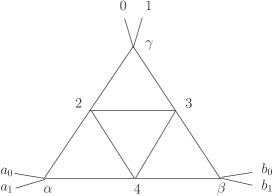
Figure 1: Dipole pair density $n^{2}_{Y}$ in an onium state with initial size $\rho=\rho_{0}-\rho_{1}$ and two children dipoles having transverse separation $\rho_{a}$ and $\rho_{b}$. The left graph shows the rapidity structure of $n_{2}$, and the right graphs indicates the graphical representation of the triple pomeron vertex.

As shown in Fig. 1, the $1\Rightarrow 2$ amplitude is defined as the dipole pair density in an onium state. It involves a triple pomeron vertex which splits the upper pomeron into two descendent pomerons. In QCD dipole modelMueller:1993rr ; Mueller:1994jq ; Mueller:1994gb , following PeschanskiPeschanski:1997yx , one can write the $1\Rightarrow 2$ amplitude as

$$n_{Y}^{(2)}\left(\rho_{0}\rho_{1};\rho_{a_{0}}\rho_{a_{1}},\rho_{b_{0}}\rho_{b_{1}}\right)$$ (25)

$$= \mathop{\displaystyle\int}dhdh_{a}dh_{b}\frac{1}{\rho_{a}^{2}\rho_{b}^{2}}\mathop{\displaystyle\int}\frac{d\omega}{2\pi i}\frac{e^{\omega Y}}{\omega-\omega\left(n,\nu\right)}\frac{\frac{\alpha N_{c}}{\pi}}{\omega-\omega\left(a\right)-\omega\left(b\right)}$$

$$\times\mathop{\displaystyle\int}d^{2}\rho_{\alpha}d^{2}\rho_{\beta}d^{2}\rho_{\gamma}E^{h,\overline{h}}\left(\rho_{0\gamma},\rho_{1\gamma}\right)E^{h_{a},\overline{h}_{b}}\left(\rho_{a_{0}\alpha},\rho_{a_{1}\alpha}\right)E^{h_{b},\overline{h}_{b}}\left(\rho_{b_{0}\beta},\rho_{b_{1}\beta}\right)$$

$$\times\mathop{\displaystyle\int}\frac{d^{2}\rho_{2}d^{2}\rho_{3}d^{2}\rho_{4}}{\left|\rho_{23}\rho_{34}\rho_{42}\right|^{2}}E^{h,\overline{h}\ast}\left(\rho_{2\gamma},\rho_{3\gamma}\right)E^{h_{a},\overline{h}_{b}\ast}\left(\rho_{2\alpha},\rho_{4\alpha}\right)\overline{E}^{h_{b},\overline{h}_{b}\ast}\left(\rho_{3\beta},\rho_{4\beta}\right),$$

$$= \mathop{\displaystyle\int}dhdh_{a}dh_{b}\frac{1}{\rho_{a}^{2}\rho_{b}^{2}}\int_{0}^{Y}\frac{\alpha N_{c}}{\pi}dy\exp\left[\omega\left(n,\nu\right)\left(Y-y\right)+\left(\omega\left(a\right)+\omega\left(b\right)\right)y\right]$$

$$\times\mathop{\displaystyle\int}d^{2}\rho_{\alpha}d^{2}\rho_{\beta}d^{2}\rho_{\gamma}E^{h,\overline{h}}\left(\rho_{0\gamma},\rho_{1\gamma}\right)E^{h_{a},\overline{h}_{b}}\left(\rho_{a_{0}\alpha},\rho_{a_{1}\alpha}\right)E^{h_{b},\overline{h}_{b}}\left(\rho_{b_{0}\beta},\rho_{b_{1}\beta}\right)$$

$$\times\mathop{\displaystyle\int}\frac{d^{2}\rho_{2}d^{2}\rho_{3}d^{2}\rho_{4}}{\left|\rho_{23}\rho_{34}\rho_{42}\right|^{2}}E^{h,\overline{h}\ast}\left(\rho_{2\gamma},\rho_{3\gamma}\right)E^{h_{a},\overline{h}_{b}\ast}\left(\rho_{2\alpha},\rho_{4\alpha}\right)\overline{E}^{h_{b},\overline{h}_{b}\ast}\left(\rho_{3\beta},\rho_{4\beta}\right)$$

with $\rho_{a}=\rho_{a_{0}}-\rho_{a_{1}}$, $\rho_{b}=\rho_{b_{0}}-\rho_{b_{1}}$ and

$$\omega\left(a\right) = \frac{4\alpha C_{F}}{\pi}\left[\psi\left(1\right)-\frac{1}{2}\psi\left(\frac{1+\left|n_{a}\right|}{2}+i\nu_{a}\right)-\frac{1}{2}\psi\left(\frac{1+\left|n_{a}\right|}{2}-i\nu_{a}\right)\right],$$

$$\omega\left(b\right) = \frac{4\alpha C_{F}}{\pi}\left[\psi\left(1\right)-\frac{1}{2}\psi\left(\frac{1+\left|n_{b}\right|}{2}+i\nu_{b}\right)-\frac{1}{2}\psi\left(\frac{1+\left|n_{b}\right|}{2}-i\nu_{b}\right)\right].$$ (26)

We also use a compact notation,

$$\int dh=\sum_{n=-\infty}^{\infty}\int d\nu\frac{2\nu^{2}+n^{2}/2}{\pi^{4}}.$$ (27)

Essentially, the above expression for $n_{Y}^{(2)}$ is the same as the ones in ref. Braun:1997nu ; Hatta:2007fg . On the other hand, hereafter, we employ different methods of evaluation and show that there exists a different anomalous dimension in $n_{Y}^{(2)}$ other than the typical pomeron anomalous dimension $\gamma=1/2$.

First of all, the last line of the above definition of $n_{Y}^{(2)}$ can be defined and written as

$$\overline{R}_{\gamma,\alpha,\beta}^{h,h_{a},h_{b}} = R_{\gamma,\alpha,\beta}^{1-h,1-h_{a},1-h_{b}},$$ (28)

$$= \mathop{\displaystyle\int}\frac{d^{2}\rho_{2}d^{2}\rho_{3}d^{2}\rho_{4}}{\left|\rho_{23}\rho_{34}\rho_{42}\right|^{2}}E^{h,\overline{h}\ast}\left(\rho_{2\gamma}\rho_{3\gamma}\right)E^{h_{a},\overline{h}_{b}\ast}\left(\rho_{2\alpha}\rho_{4\alpha}\right)\overline{E}^{h_{b},\overline{h}_{b}\ast}\left(\rho_{3\beta}\rho_{4\beta}\right).$$

After using the $SL\left(2,C\right)$ transformation

$$\rho^{\prime}=\frac{\rho_{\beta}-\rho_{\gamma}}{\rho_{\beta}-\rho_{\alpha}}\frac{\rho-\rho_{\alpha}}{\rho-\rho_{\gamma}},$$ (29)

one can easily write

$$R_{\gamma,\alpha,\beta}^{1-h,1-h_{a},1-h_{b}}=g_{3P}\left(1-h,1-h_{a},1-h_{b}\right)\left(\rho_{\alpha\beta}^{-1+i}\rho_{\beta\gamma}^{-1+j}\rho_{\gamma\alpha}^{-1+k}\right)\left(\overline{\rho}_{\alpha\beta}^{-1+\overline{i}}\overline{\rho}_{\beta\gamma}^{-1+\overline{j}}\overline{\rho}_{\gamma\alpha}^{-1+\overline{k}}\right),$$ (30)

where

$$i = -h+h_{a}+h_{b},$$ (31)

$$j = -h_{a}+h_{b}+h,$$ (32)

$$k = -h_{b}+h_{a}+h,$$ (33)

and

$$g_{3P}\left(h,h_{a},h_{b}\right) = \mathop{\displaystyle\int}\frac{d^{2}\rho_{2}d^{2}\rho_{3}d^{2}\rho_{4}}{\left|\rho_{23}\rho_{34}\rho_{42}\right|^{2}}\rho_{23}^{h}\overline{\rho}_{23}^{\overline{h}}\left(\frac{\rho_{24}}{\rho_{2}\rho_{4}}\right)^{h_{a}}\left(\frac{\overline{\rho}_{24}}{\overline{\rho}_{2}\overline{\rho}_{4}}\right)^{\overline{h}_{a}}$$ (34)

$$\times\left(\frac{\rho_{34}}{\left(1-\rho_{3}\right)\left(1-\rho_{4}\right)}\right)^{h_{b}}\left(\frac{\overline{\rho}_{34}}{\left(1-\overline{\rho}_{3}\right)\left(1-\overline{\rho}_{4}\right)}\right)^{\overline{h}_{b}}$$

Explicit evaluation of $g_{3P}$ can be found in ref. (Korchemsky:1997fy ) and Appendix F.

Furthermore, according to the Fourier transform of $E^{h,\overline{h}}\left(\rho_{0\gamma}\rho_{1\gamma}\right)$, one can get rid of the impact parameter dependence and define $n_{Y}^{(2)}$ in momentum space,

$$n_{Y,Q,q_{a},q_{b}}^{(2)\rho,\rho_{a},\rho_{b}} = \int d^{2}rd^{2}r_{a}d^{2}r_{b}e^{iQr+q_{a}r_{a}+iq_{b}r_{b}}n_{Y}^{(2)}\left(\rho_{0}\rho_{1};\rho_{a_{0}}\rho_{a_{1}},\rho_{b_{0}}\rho_{b_{1}}\right)$$ (35)

$$= \mathop{\displaystyle\int}dhdh_{a}dh_{b}\frac{1}{\rho_{a}^{2}\rho_{b}^{2}}\mathop{\displaystyle\int}\frac{d\omega}{2\pi i}\frac{e^{\omega Y}}{\omega-\omega\left(n,\nu\right)}\frac{\frac{\alpha N_{c}}{\pi}}{\omega-\omega\left(a\right)-\omega\left(b\right)}$$

$$\times\frac{b_{n,\nu}b_{n_{a},\nu_{a}}b_{n_{b},\nu_{b}}\left|\rho\rho_{a}\rho_{b}\right|}{\left(2\pi^{2}\right)^{3}}E_{Q}^{n,\nu}\left(\rho\right)E_{q_{a}}^{n_{a},\nu_{a}}\left(\rho_{a}\right)E_{q_{b}}^{n_{b},\nu_{b}}\left(\rho_{b}\right)g_{3P}\left(1-h,1-h_{a},1-h_{b}\right)$$

$$\times\mathop{\displaystyle\int}d^{2}\rho_{\alpha}d^{2}\rho_{\beta}d^{2}\rho_{\gamma}\exp\left(iQ\rho_{\gamma}+iq_{a}\rho_{\alpha}+iq_{b}\rho_{\beta}\right)\left[\rho_{\alpha\beta}^{-1+i}\rho_{\beta\gamma}^{-1+j}\rho_{\gamma\alpha}^{-1+k}\right]\left[a.h.\right]$$

where a.h. stands for the antiholomorphic part of the square-bracket term, $r=\frac{1}{2}\left(\rho_{0}+\rho_{1}\right)$, $r_{a}=\frac{1}{2}\left(\rho_{a_{0}}+\rho_{a_{1}}\right)$ and $r_{b}=\frac{1}{2}\left(\rho_{b_{0}}+\rho_{b_{1}}\right)$. Hereafter in this section, we compute $n_{Y}^{(2)}$ in $\rho^{2}q_{a}^{2}\ll 1$ limit, where $q_{a}^{2}$, $q_{b}^{2}$ and $Q^{2}$ are of the same order and $\rho$, $\rho_{a}$ and $\rho_{b}$ are of the same order as well.

In addition, let us define

$$I_{Q,q_{a},q_{b}}^{h,h_{a},h_{b}}=\mathop{\displaystyle\int}d^{2}\rho_{\alpha}d^{2}\rho_{\beta}d^{2}\rho_{\gamma}\exp\left(iQ\rho_{\gamma}+iq_{a}\rho_{\alpha}+iq_{b}\rho_{\beta}\right)\left[\rho_{\alpha\beta}^{-1+i}\rho_{\beta\gamma}^{-1+j}\rho_{\gamma\alpha}^{-1+k}\right]\left[a.h.\right]$$ (36)

In order to evaluate $I_{Q,q_{a},q_{b}}^{h,h_{a},h_{b}}$, we change the variables $\rho_{\alpha}$, $\rho_{\beta}$ and $\rho_{\gamma}$ into $u$, $v$ and $w$, where

$$u = \frac{1}{2}\left(\rho_{\alpha}+\rho_{\beta}\right),$$

$$v = \rho_{\alpha}-\rho_{\beta},$$

$$w = \rho_{\alpha}-\rho_{\gamma}+\rho_{\beta}-\rho_{\gamma}.$$ (37)

Then the integral can be cast into,

$$I_{Q,q_{a},q_{b}}^{h,h_{a},h_{b}} = \frac{1}{4}\mathop{\displaystyle\int}d^{2}ud^{2}vd^{2}w\exp\left(i\left(Q+q_{a}+q_{b}\right)u-iQ\frac{w}{2}+i\left(q_{a}-q_{b}\right)\frac{v}{2}\right)$$ (38)

$$\times\left[v^{-1+i}\left(\frac{w-v}{2}\right)^{-1+j}\left(\frac{w+v}{2}\right)^{-1+k}\right]\left[a.h.\right],$$

$$= \pi^{2}\delta^{\left(2\right)}\left(Q+q_{a}+q_{b}\right)\mathop{\displaystyle\int}d^{2}vd^{2}w\exp\left(-iQ\cdot\frac{w}{2}+i\left(q_{a}-q_{b}\right)\cdot\frac{v}{2}\right)$$

$$\times\left[v^{-1+i}\left(\frac{w-v}{2}\right)^{-1+j}\left(\frac{w+v}{2}\right)^{-1+k}\right]\left[a.h.\right],$$

where the factor of $\frac{1}{4}$ comes from the Jacobian. Hereafter, in order to simplify the calculation, we define

$$I_{Q,q_{a},q_{b}}^{h,h_{a},h_{b}}=\pi^{2}\delta^{\left(2\right)}\left(Q+q_{a}+q_{b}\right)I_{Q,q_{-}}^{h,h_{a},h_{b}},$$ (39)

with $q_{-}=\frac{1}{2}\left(q_{a}-q_{b}\right)$, perform the Taylor expansion of the term $\exp\left(-iQ\frac{w}{2}\right)$ and only keep the first term. Keeping only the first term is equivalent to the physical case when $Q=0$ and $q_{a}=-q_{b}=q$ which corresponds to the forward scattering of an onium on two nucleons. We put the evaluation of $I_{Q,q_{-}}^{h,h_{a},h_{b}}$ and discussion of higher order terms in the expansion in Appendix A and B, respectively. As shown in the appendix, the following conclusion holds for all the terms in the expansion when $n=0$.

Therefore, one obtains,

$$n_{Y,Q,q_{-},0}^{(2)\rho,\rho_{a},\rho_{b}} = \mathop{\displaystyle\int}dhdh_{a}dh_{b}\frac{1}{\rho_{a}^{2}\rho_{b}^{2}}\int_{0}^{Y}\frac{\alpha N_{c}}{\pi}dy\exp\left[\omega\left(n,\nu\right)\left(Y-y\right)+\left(\omega\left(a\right)+\omega\left(b\right)\right)y\right]$$ (40)

$$\times\frac{b_{n,\nu}b_{n_{a},\nu_{a}}b_{n_{b},\nu_{b}}\left|\rho\rho_{a}\rho_{b}\right|}{\left(2\pi^{2}\right)^{3}}E_{Q}^{n,\nu}\left(\rho\right)E_{q_{a}}^{n_{a},\nu_{a}}\left(\rho_{a}\right)E_{q_{b}}^{n_{b},\nu_{b}}\left(\rho_{b}\right)g_{3P}\left(1-h,1-h_{a},1-h_{b}\right)$$

$$\times 4\pi^{2}\left(\frac{2}{q_{-}}\right)^{i+j+k+\overline{i}+\overline{j}+\overline{k}-2}\frac{\Gamma\left(k\right)\Gamma\left(j\right)}{\Gamma\left(k+j\right)}\frac{\Gamma\left(1-\overline{j}-\overline{k}\right)}{\Gamma\left(1-\overline{j}\right)\Gamma\left(1-\overline{k}\right)}\frac{\Gamma\left(i+j+k-1\right)}{\Gamma\left(2-\overline{i}-\overline{j}-\overline{k}\right)}$$

where the last subscript of $n_{Y,Q,q_{-},0}^{(2)\rho,\rho_{a},\rho_{b}}$ means that this result comes from the first term of the expansion. Assuming that the diffusion approximation is valid which requires $\ln^{2}\left(q\rho\right)\ll\frac{14\alpha C_{F}\zeta\left(3\right)}{\pi}Y$, let us first evaluate the rapidity-integral. The integral yields

$$\frac{\frac{\alpha N_{c}}{\pi}}{\omega\left(n,\nu\right)-\omega\left(a\right)-\omega\left(b\right)}\left\{\exp\left[\left(\omega\left(a\right)+\omega\left(b\right)\right)Y\right]-\exp\left[\omega\left(n,\nu\right)Y\right]\right\}.$$ (41)

For the first term, the saddle point approximation fixes $h_{a}=h_{b}=\frac{1}{2}$, $n_{a}=n_{b}=0$. As a result, $n_{Y}^{(2)}$ is then proportional to $\exp\left[2\left(\alpha_{P}-1\right)Y\right]$. In comparison, for the second term, $n_{Y}^{(2)}$ is proportional to $\exp\left[\left(\alpha_{P}-1\right)Y\right]$ because saddle point approximation fixes $h=\frac{1}{2}$ and $n=0$. Therefore, we can drop the second term in later discussions since it is the next-leading order contribution which is exponentially suppressed.

In the following, we break the discussions into two parts. The first part is on the $n=0$ case, and the second part discusses the result when $n\neq 0$. Usually, we can neglect the contribution from sub-dominant trajectories of pomerons when rapidity is large enough as we explained in the calculation of the single pomeron exchange amplitude. Nevertheless, the rapidity interval of the upper pomeron after integration is infinitesimal in this situation. Therefore, we have to seriously consider the contribution from sub-dominant trajectories.

III.1 $n=0$ part

$n=0$ part of the amplitude is the only angular-independent part. From Appendix C, one uses saddle point approximation to evaluate $\mathop{\displaystyle\int}dh_{a}dh_{b}$ integrals,

$$\mathop{\displaystyle\int}dh_{a}\frac{b_{n_{a},\nu_{a}}\left|\rho_{a}\right|}{2\pi^{2}}E_{q_{a}}^{n_{a},\nu_{a}}\left(\rho_{a}\right)\left(\frac{4}{q^{2}}\right)^{\gamma_{a}}\exp\left[\omega\left(a\right)Y\right]$$ (42)

$$\simeq \frac{1}{2\pi}\frac{\rho_{a}}{q}e\left(\rho_{a},q_{a}\right)\frac{\exp\left[\left(\alpha_{P}-1\right)Y\right]\exp\left[-\frac{\pi\ln^{2}\left(\rho_{a}q_{a}\right)}{28\alpha C_{F}\zeta\left(3\right)Y}\right]}{\left(7\alpha\zeta\left(3\right)C_{F}Y\right)^{3/2}},$$

where $\gamma_{a}=\frac{1}{2}\left(h_{a}+\overline{h}_{a}\right)=\frac{1}{2}+i\nu_{a}$. In the end, there is only $\mathop{\displaystyle\int}dh$ left in the expression,

$$n_{Y,Q,q_{-},0}^{(2)\rho,\rho_{a},\rho_{b}} \simeq \mathop{\displaystyle\int}dh\frac{1}{2\rho_{a}^{2}\rho_{b}^{2}}\frac{1}{2\chi\left(\frac{1}{2}\right)-\chi\left(\gamma\right)}\frac{b_{0,\nu}\left|\rho\right|}{2\pi^{2}}E_{Q}^{0,\nu}\left(\rho\right)g_{3P}\left(1-\gamma,\frac{1}{2},\frac{1}{2}\right)$$ (43)

$$\times 4\pi^{2}\left(\frac{4}{q_{-}^{2}}\right)^{\gamma-1}\frac{\Gamma^{3}\left(\gamma\right)\Gamma\left(1-2\gamma\right)}{\Gamma\left(2\gamma\right)\Gamma^{3}\left(1-\gamma\right)}$$

$$\times\frac{1}{4\pi^{2}}\frac{\rho_{a}\rho_{b}}{q_{-}^{2}}e\left(\rho_{a},q_{a}\right)e\left(\rho_{b},q_{b}\right)\frac{\exp\left[2\left(\alpha_{P}-1\right)Y\right]\exp\left[-\frac{\pi\left(\ln^{2}\left(q_{a}\rho_{a}\right)+\ln^{2}\left(q_{b}\rho_{b}\right)\right)}{28\alpha C_{F}\zeta\left(3\right)Y}\right]}{\left(7\alpha\zeta\left(3\right)C_{F}Y\right)^{3}}$$

Let us focus on the $dh$-integral (first two lines of the above expression):

$$\frac{4\pi^{2}}{2\rho_{a}^{2}\rho_{b}^{2}}\mathop{\displaystyle\int}dh\frac{1}{2\chi\left(\frac{1}{2}\right)-\chi\left(\gamma\right)}\frac{b_{0,\nu}\left|\rho\right|}{2\pi^{2}}E_{Q}^{0,\nu}\left(\rho\right)g_{3P}\left(1-\gamma,\frac{1}{2},\frac{1}{2}\right)\left(\frac{4}{q_{-}^{2}}\right)^{\gamma-1}\frac{\Gamma^{3}\left(\gamma\right)\Gamma\left(1-2\gamma\right)}{\Gamma\left(2\gamma\right)\Gamma^{3}\left(1-\gamma\right)},$$ (44)

$$= \frac{2}{\rho_{a}^{2}\rho_{b}^{2}}\int\frac{d\gamma}{2\pi i}\frac{\left|\rho\right|}{2\chi\left(\frac{1}{2}\right)-\chi\left(\gamma\right)}E_{Q}^{n,\nu}\left(\rho\right)g_{3P}\left(1-\gamma,\frac{1}{2},\frac{1}{2}\right)\left(\frac{4}{q_{-}^{2}}\right)^{\gamma-1}\frac{\Gamma\left(\gamma\right)}{\Gamma\left(1-\gamma\right)}.$$

In $\rho Q\ll 1$ limitNavelet:1997xn ,

$$E_{Q}^{0,\nu}\left(\rho\right)\simeq\rho^{1-2\gamma}-\frac{Q^{2\gamma-1}\Gamma^{2}\left(\frac{3}{2}-\gamma\right)2^{6-12\gamma}}{\Gamma^{2}\left(\frac{1}{2}+\gamma\right)}\left(\rho Q\right)^{2\gamma-1}.$$ (45)

Therefore, the integral can be cast into the form

$$dh-integral \simeq \frac{2}{\rho_{a}^{2}\rho_{b}^{2}}\int_{\frac{1}{2}-i\infty}^{\frac{1}{2}+i\infty}\frac{d\gamma}{2\pi i}\frac{1}{2\chi\left(\frac{1}{2}\right)-\chi\left(\gamma\right)}g_{3P}\left(1-\gamma,\frac{1}{2},\frac{1}{2}\right)\frac{\Gamma\left(\gamma\right)}{\Gamma\left(1-\gamma\right)}\left(\frac{4}{\rho^{2}q_{-}^{2}}\right)^{\gamma-1}$$ (46)

$$-\frac{2}{\rho_{a}^{2}\rho_{b}^{2}}\int_{\frac{1}{2}-i\infty}^{\frac{1}{2}+i\infty}\frac{d\gamma}{2\pi i}\frac{1}{2\chi\left(\frac{1}{2}\right)-\chi\left(\gamma\right)}g_{3P}\left(1-\gamma,\frac{1}{2},\frac{1}{2}\right)\frac{\Gamma\left(\gamma\right)}{\Gamma\left(1-\gamma\right)}$$

$$\times\frac{\Gamma^{2}\left(\frac{3}{2}-\gamma\right)2^{6-12\gamma}}{\Gamma^{2}\left(\frac{1}{2}+\gamma\right)}\left(\frac{4Q^{2}}{q_{-}^{2}}\right)^{2\gamma-1}\left(\frac{\rho^{2}q_{-}^{2}}{4}\right)^{\gamma}$$

Figure 2: Illustration of the contours in complex $\gamma$ plane for the computation of $n_{Y}^{(2)}$ when $n=0$.

According to the residue theorem, the contour integral equals to the sum of all residues of poles enclosed by the contour. In the $\rho^{2}q_{-}^{2}\ll 1$ limit, the first poles to the left and right of the vertical contour are the dominant contribution. The positions of these two poles are determined by the equation $2\chi\left(\frac{1}{2}\right)-\chi\left(\gamma\right)=0$, and they are $\gamma_{0}^{\left(2\right)\ast}=0.18$ and $1-\gamma_{0}^{\left(2\right)\ast}=0.82$. For the first integral(see the left graph of Fig. 2), we should close the contour to the left to $-\infty$ and compute the residue of the pole at $\gamma=0.18$; while for the second integral(see the right graph of Fig. 2), we should close the contour to the right to $\infty$ and compute the residue at $\gamma=0.82$. Eventually, up to leading order precision, one reaches the result

$$n_{Y,Q,q_{a},q_{b},0}^{(2)\rho,\rho_{a},\rho_{b}} = \pi^{2}\delta^{\left(2\right)}\left(Q+q_{a}+q_{b}\right)n_{Y,Q,q_{-},0}^{(2)\rho,\rho_{a},\rho_{b}}$$ (47)

$$\simeq \frac{1}{2\rho_{a}q_{-}\rho_{b}q_{-}}\left(\frac{\rho^{2}q_{-}^{2}}{4}\right)^{1-\gamma_{0}^{\left(2\right)\ast}}\delta^{\left(2\right)}\left(Q+q_{a}+q_{b}\right)\frac{g_{3P}\left(1-\gamma_{0}^{\left(2\right)\ast},\frac{1}{2},\frac{1}{2}\right)}{\left|\chi^{\prime}\left(\gamma_{0}^{\left(2\right)\ast}\right)\right|}$$

$$\times\left[\frac{\Gamma\left(\gamma_{0}^{\left(2\right)\ast}\right)}{\Gamma\left(1-\gamma_{0}^{\left(2\right)\ast}\right)}-\frac{\Gamma\left(1-\gamma_{0}^{\left(2\right)\ast}\right)}{\Gamma\left(\gamma_{0}^{\left(2\right)\ast}\right)}\frac{\Gamma^{2}\left(\frac{1}{2}+\gamma_{0}^{\left(2\right)\ast}\right)2^{-6+12\gamma_{0}^{\left(2\right)\ast}}}{\Gamma^{2}\left(\frac{3}{2}-\gamma_{0}^{\left(2\right)\ast}\right)}\left(\frac{4Q^{2}}{q_{-}^{2}}\right)^{-2\gamma_{0}^{\left(2\right)\ast}+1}\right]$$

$$\times e\left(\rho_{a},q_{a}\right)e\left(\rho_{b},q_{b}\right)\frac{\exp\left[2\left(\alpha_{P}-1\right)Y\right]\exp\left[-\frac{\pi\left(\ln^{2}\left(q_{a}\rho_{a}\right)+\ln^{2}\left(q_{b}\rho_{b}\right)\right)}{28\alpha C_{F}\zeta\left(3\right)Y}\right]}{\left(7\alpha\zeta\left(3\right)C_{F}Y\right)^{3}}.$$

In this leading order calculation of $1\Rightarrow 2$ amplitude, we push the rapidity integration to its upper limit $Y$ which leaves infinitesimal rapidity for the upper pomeron. As a result, the anomalous dimensions is determined by the dynamical pole introduced by the rapidity integration. This result agrees with eq.(44) in ref.Mueller:1994jq .

$$n_{2}\left(Y,x_{01},q\right) = \frac{\pi x_{01}^{2}\exp\left[2\left(\alpha_{P}-1\right)Y\right]}{8\left(7\alpha\zeta\left(3\right)C_{F}Y\right)^{3}}\int_{-\infty}^{+\infty}\frac{d\nu}{2\pi}\left(qx_{01}\right)^{2i\nu-1}\frac{V_{\nu}}{4\ln 2-\chi\left(\nu\right)}$$ (48)

$$\simeq \frac{\pi\exp\left[2\left(\alpha_{P}-1\right)Y\right]}{8\left(7\alpha\zeta\left(3\right)C_{F}Y\right)^{3}}\frac{\left(q^{2}x_{01}^{2}\right)^{0.82}}{q^{2}}\frac{V_{\nu_{0}^{(2)\ast}}}{\left|\chi^{\prime}\left(\nu_{0}^{(2)\ast}\right)\right|},$$ (49)

where $V_{\nu}$ is defined by

$$\int_{-\infty}^{+\infty}\frac{d\nu}{2\pi}\left(qx_{01}\right)^{2i\nu-1}V_{\nu}=\int\frac{d^{2}x_{2}}{x_{01}x_{12}}J_{0}\left(\frac{1}{2}qx_{01}\right)e\left(x_{12},q\right)e\left(x_{02},q\right),$$ (50)

and

$$\gamma_{0}^{\left(2\right)\ast\prime}=\frac{1}{2}+i\nu_{0}^{\left(2\right)\ast}=0.82.$$ (51)

In reaching the final result, we have assumed that $V_{\nu}$ has no pole before $\gamma_{0}^{\left(2\right)\ast\prime}$. The proof of this assumption is explicitly provided in appendix D.

III.2 $n\neq 0$ part

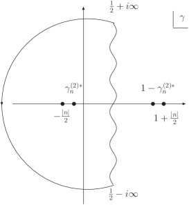
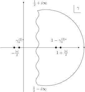
Figure 3: Illustration of the contours in complex $\gamma$ plane for the computation of $n_{Y}^{(2)}$ when $n\neq 0$.

$n\neq 0$ part of the amplitude is angular-dependent, and it vanishes after averaging over the angle of initial dipole orientation. This part of amplitude comes from the subdominant trajectories of the upper pomeron. As discussed in Appendix B, we should restrict ourselves to the forward scattering case in which $Q=0$, since we are unable to prove that the whole discussion can be generalized to arbitrary momenta. According to the discussion above, one can easily obtain the expression for $n_{Y}^{\left(2\right)}$ for nonzero value of $n$ in forward scattering.

$$\left.n_{Y,Q=0,q_{-}}^{(2)\rho,\rho_{a},\rho_{b}}\right|_{\left|n\right|>0} \simeq \mathop{\displaystyle\int}_{n\neq 0}dh\frac{b_{n,\nu}\left|\rho\right|}{\rho_{a}^{2}\rho_{b}^{2}}\frac{1}{2\chi\left(\frac{1}{2}\right)-\chi\left(n,\gamma\right)}E_{0}^{n,\nu}\left(\rho\right)g_{3P}\left(1-h,\frac{1}{2},\frac{1}{2}\right)\left(\frac{4}{q_{-}^{2}}\right)^{\gamma-1}\frac{\Gamma^{3}\left(h\right)\Gamma\left(1-2\overline{h}\right)}{\Gamma\left(2h\right)\Gamma^{3}\left(1-\overline{h}\right)}$$ (52)

$$\times\frac{1}{4\pi^{2}}\frac{\rho_{a}\rho_{b}}{q_{-}^{2}}e\left(\rho_{a},q_{a}\right)e\left(\rho_{b},q_{b}\right)\frac{\exp\left[2\left(\alpha_{P}-1\right)Y\right]\exp\left[-\frac{\pi\left(\ln^{2}\left(q_{a}\rho_{a}\right)+\ln^{2}\left(q_{b}\rho_{b}\right)\right)}{28\alpha C_{F}\zeta\left(3\right)Y}\right]}{\left(7\alpha\zeta\left(3\right)C_{F}Y\right)^{3}}$$

Changing $\mathop{\displaystyle\int}_{n\neq 0}dh$ into $\int\frac{d\gamma}{2\pi i}$, and using the identity $g_{3P}\left(1-h,\frac{1}{2},\frac{1}{2}\right)=g_{3P}\left(1-\overline{h},\frac{1}{2},\frac{1}{2}\right)$ which we proved in Appendix F, along with the detailed derivation in Appendix E, one can reach

$$\left.n_{Y,Q=0,q_{-}}^{(2)\rho,\rho_{a},\rho_{b}}\right|_{\left|n\right|>0} \simeq \sum_{n=1}^{\infty}\frac{2\left|\rho\right|}{\rho_{a}^{2}\rho_{b}^{2}}\int_{\frac{1}{2}-i\infty}^{\frac{1}{2}+i\infty}\frac{d\gamma}{2\pi i}\frac{1}{2\chi\left(\frac{1}{2}\right)-\chi\left(n,\gamma\right)}\frac{\Gamma\left(\gamma+\frac{\left|n\right|}{2}\right)}{\Gamma\left(1+\frac{\left|n\right|}{2}-\gamma\right)}\left(\frac{4}{q_{-}^{2}}\right)^{\gamma-1}$$ (53)

$$\times i^{\left|n\right|}\left[E_{0}^{n,\nu}\left(\rho\right)+E_{0}^{-n,\nu}\left(\rho\right)\right]g_{3P}\left(1-h,\frac{1}{2},\frac{1}{2}\right)$$

$$\times\frac{1}{4\pi^{2}}\frac{\rho_{a}\rho_{b}}{q_{-}^{2}}e\left(\rho_{a},q_{a}\right)e\left(\rho_{b},q_{b}\right)\frac{\exp\left[2\left(\alpha_{P}-1\right)Y\right]\exp\left[-\frac{\pi\left(\ln^{2}\left(q_{a}\rho_{a}\right)+\ln^{2}\left(q_{b}\rho_{b}\right)\right)}{28\alpha C_{F}\zeta\left(3\right)Y}\right]}{\left(7\alpha\zeta\left(3\right)C_{F}Y\right)^{3}}$$

In $\rho Q\ll 1$ limitNavelet:1997xn ,

$$E_{Q}^{n,\nu}\left(\rho\right) = \overline{Q}^{i\nu-n/2}Q^{i\nu+n/2}2^{-6i\nu}\Gamma\left(1-i\nu+\frac{\left|n\right|}{2}\right)\Gamma\left(1-i\nu-\frac{\left|n\right|}{2}\right)$$

$$\times\left[J_{\frac{n}{2}-i\nu}\left(\frac{\overline{Q}\rho}{4}\right)J_{-\frac{n}{2}-i\nu}\left(\frac{\overline{\rho}Q}{4}\right)-\left(-1\right)^{n}J_{-\frac{n}{2}+i\nu}\left(\frac{\overline{Q}\rho}{4}\right)J_{\frac{n}{2}+i\nu}\left(\frac{\overline{\rho}Q}{4}\right)\right]$$

$$\simeq \left(\frac{\rho}{\overline{\rho}}\right)^{\frac{n}{2}}\rho^{1-2\gamma}-\left(-1\right)^{n}\frac{Q^{2\gamma-1}\Gamma\left(\frac{3}{2}-\gamma+\frac{n}{2}\right)\Gamma\left(\frac{3}{2}-\gamma-\frac{n}{2}\right)2^{6-12\gamma}}{\Gamma\left(\frac{1}{2}+\gamma+\frac{n}{2}\right)\Gamma\left(\frac{1}{2}+\gamma-\frac{n}{2}\right)}\left(\frac{Q}{\overline{Q}}\right)^{n}\left(\frac{\rho}{\overline{\rho}}\right)^{-\frac{n}{2}}\left(\rho Q\right)^{2\gamma-1}.$$ (55)

where $\left(\frac{\rho}{\overline{\rho}}\right)^{\frac{n}{2}}$ and $\left(\frac{\rho}{\overline{\rho}}\right)^{-\frac{n}{2}}$ parts give the angular dependence, and vanish after averaging. Thus, $E_{0}^{n,\nu}\left(\rho\right)+E_{0}^{-n,\nu}\left(\rho\right)=\left[\left(\frac{\rho}{\overline{\rho}}\right)^{\frac{n}{2}}+\left(\frac{\rho}{\overline{\rho}}\right)^{-\frac{n}{2}}\right]\rho^{1-2\gamma}$. Similarly, one has to examine the pole structure of the integrand of the $\gamma$ integral. Assuming that $g_{3P}\left(1-h,\frac{1}{2},\frac{1}{2}\right)$ does not contribute any new singularity in the domain $\left(-\frac{\left|n\right|}{2},\frac{\left|n\right|}{2}+1\right)$(see Appendix F), noting that $\chi\left(\gamma,n\right)$ is analytic in the strip $-\frac{\left|n\right|}{2}<\mathop{\mathrm{R}e}\nu<\frac{\left|n\right|}{2}+1$, and defining $\gamma_{n}^{\left(2\right)\ast}$ as the solution to the equations $2\chi\left(\frac{1}{2}\right)-\chi\left(n,\gamma\right)=0$ in the domain $\left(-\frac{\left|n\right|}{2},\frac{1}{2}\right)$(see the left graph of Fig.3), one reaches

$$\left.n_{Y,Q=0,q_{-}}^{(2)\rho,\rho_{a},\rho_{b}}\right|_{n}\propto\frac{\left(\rho^{2}q_{-}^{2}\right)^{1-\gamma_{n}^{\left(2\right)\ast}}}{\rho_{a}q_{-}\rho_{b}q_{-}}e\left(\rho_{a},q_{a}\right)e\left(\rho_{b},q_{b}\right)\frac{\exp\left[2\left(\alpha_{P}-1\right)Y\right]\exp\left[-\frac{\pi\left(\ln^{2}\left(q_{a}\rho_{a}\right)+\ln^{2}\left(q_{b}\rho_{b}\right)\right)}{28\alpha C_{F}\zeta\left(3\right)Y}\right]}{\left(7\alpha\zeta\left(3\right)C_{F}Y\right)^{3}}$$ (56)

by closing the contour to the left to $-\infty$ and collecting the residue at $\gamma=\gamma_{n}^{\left(2\right)\ast}$ (other residues are suppressed by factors of $\rho^{2}q_{-}^{2}$). It seems that the dynamical pole introduced by the rapidity integrations always comes before other poles. Here we conjecture that, although we can not prove, $\left.n_{Y,Q=0,q_{-}}^{(2)\rho,\rho_{a},\rho_{b}}\right|_{n}\propto\frac{\left(\rho^{2}q_{-}^{2}\right)^{1-\gamma_{n}^{\left(2\right)\ast}}}{\rho_{a}q_{-}\rho_{b}q_{-}}$ still holds even for nonzero momenta of $Q$ by picking up poles at $\gamma_{n}^{\left(2\right)\ast}$ or $1-\gamma_{n}^{\left(2\right)\ast}$ depending on how the contour is closed(as shown in both graphs of Fig. 3).

Comparing this result to the result in the case of $n=0$, one can spot that $n_{Y}^{(2)}$ with nonzero $n$ is suppressed by factors of $\rho^{2}q_{-}^{2}$ in the $\rho^{2}q_{-}^{2}\ll 1$ limit since $1-\gamma_{n}^{\left(2\right)\ast}\simeq 1+\frac{\left|n\right|}{2}-\epsilon_{n}$, where $\epsilon_{n}$ is a small positive number. Therefore, the sub-dominant trajectories can be neglected in the case of forward scattering computation. It is our conjecture that they can also be neglected in the non-forward scattering case. This result is new.

To summarize, we have shown that the dipole pair density in momentum space scales as $\left(\rho^{2}q^{2}\right)^{1-\gamma_{0}^{\left(2\right)\ast}}$ with respect to the onium size in $\rho^{2}q^{2}\ll 1$ limit. This indicates that the anomalous dimension of dipole pair density is equal to $0.18$. Similar result can also be found in ref. (Navelet:2002zz ). Qualitatively, this result is easy to understand according to the discussion in Section II. The anomalous dimension is determined by the upper pomeron which connects the triple pomeron vertex to the initial onium as seen in fig. 1. The rapidity length of the upper pomeron is infinitesimal after rapidity integration. The anomalous dimension should approach zero in small rapidity limit or DGLAP limit ($\rho^{2}q^{2}\ll 1$ implies the collinear ordering and the evolution in virtuality). In the case of onium-onium scattering, the double pomeron exchange amplitude between two onia with sizes $\rho$ and $\rho^{\prime}$ then scales as

$$F^{\left(2\right)}\left(\rho,\rho^{\prime},q,Y\right)\propto\left(q^{2}\rho^{2}\right)^{0.82}\left(q^{2}\rho^{\prime 2}\right)^{0.82}\left\{\alpha^{2}\frac{\exp\left[\left(\alpha_{P}-1\right)Y\right]}{\left(7\alpha\zeta\left(3\right)C_{F}Y\right)^{3/2}}\right\}^{2}.$$ (57)

IV The $1\Rightarrow 3$ amplitude and Triple pomeron exchange.

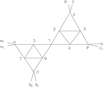
Figure 4: Dipole triplet density $n_{Y}^{3}$ in an onium state with initial size $\rho=\rho_{0}-\rho_{1}$ and three children dipoles having transverse separation $\rho_{a}$, $\rho_{b}$ and $\rho_{c}$. The left graph shows the rapidity structure of $n_{3}$, and the right graphs indicates the graphical representation of two successive triple pomeron vertices.

As shown in Fig. 4, the $1\Rightarrow 3$ amplitude is defined as the dipole triplet density in an onium state. It is easy to generalize the $1\Rightarrow 2$ amplitude to the $1\Rightarrow 3$ amplitude by adding one more triple-pomeron vertex. This amplitude corresponds to the graph in which one ancestor pomeron splits into two pomersons and one of the two descendent pomerons again splits into another two pomerons. As discussed in ref. Braun:1997nu , the amplitude of this graph is different from the $1\Rightarrow 3$ amplitude introduced in ref. Peschanski:1997yx which involves a non-local $1\Rightarrow 3$ pomeron vertex(see also ref. Janik:1999fk ). As seen in ref. Peschanski:1997yx , an initial pomeron can split into $p$ ($p>1$) pomerons simultaneously via a non-local $1\Rightarrow p$ pomeron vertex. The use of the non-local $1\Rightarrow p$ pomeron vertex ($p>1$) is still under debateBraun:1997nu . It seems more natural that the theory only requires one type of vertex (triple pomeron vertex) instead of infinite number of different vertices. Therefore, the $1\Rightarrow 3$ amplitude reads,

$$n_{Y}^{(3)}\left(\rho_{0}\rho_{1};\rho_{a_{0}}\rho_{a_{1}},\rho_{b_{0}}\rho_{b_{1}},\rho_{c_{0}}\rho_{c_{1}}\right)$$ (58)

$$= \frac{1}{\rho_{a}^{2}\rho_{b}^{2}\rho_{c}^{2}}\mathop{\displaystyle\int}dhdh_{a}dh_{b}dh_{c}dh_{d}\mathop{\displaystyle\int}d^{2}\rho_{\alpha}d^{2}\rho_{\beta}d^{2}\rho_{\gamma}d^{2}\rho_{\theta}d^{2}\rho_{\delta}$$

$$\times\mathop{\displaystyle\int}\frac{d\omega}{2\pi i}\frac{e^{\omega Y}}{\omega-\omega\left(n,\nu\right)}\frac{\frac{\alpha N_{c}}{\pi}}{\omega-\omega\left(c\right)-\omega\left(d\right)}\frac{\frac{\alpha N_{c}}{\pi}}{\omega-\omega\left(a\right)-\omega\left(b\right)-\omega\left(c\right)}$$

$$\times E^{h,\overline{h}}\left(\rho_{0\delta}\rho_{1\delta}\right)E^{h_{c},\overline{h}_{c}}\left(\rho_{c_{0}\theta}\rho_{c_{1}\theta}\right)E^{h_{a},\overline{h}_{a}}\left(\rho_{a_{0}\alpha}\rho_{a_{1}\alpha}\right)E^{h_{b},\overline{h}_{b}}\left(\rho_{b_{0}\beta}\rho_{b_{1}\beta}\right)$$

$$\times\mathop{\displaystyle\int}\frac{d^{2}\rho_{2}d^{2}\rho_{3}d^{2}\rho_{4}}{\left|\rho_{23}\rho_{34}\rho_{42}\right|^{2}}E^{h,\overline{h}\ast}\left(\rho_{2\delta}\rho_{3\delta}\right)E^{h_{d},\overline{h}_{d}}\left(\rho_{2\gamma}\rho_{4\gamma}\right)\overline{E}^{h_{c},\overline{h}_{c}\ast}\left(\rho_{3\theta}\rho_{4\theta}\right)$$

$$\times\mathop{\displaystyle\int}\frac{d^{2}\rho_{5}d^{2}\rho_{6}d^{2}\rho_{7}}{\left|\rho_{56}\rho_{57}\rho_{67}\right|^{2}}E^{h_{d},\overline{h}_{d}\ast}\left(\rho_{5\gamma}\rho_{6\gamma}\right)E^{h_{a},\overline{h}_{a}\ast}\left(\rho_{5\alpha}\rho_{7\alpha}\right)\overline{E}^{h_{b},\overline{h}_{b}\ast}\left(\rho_{6\beta}\rho_{7\beta}\right)$$

Following the same procedure as in the last section, first of all, we define

$$\overline{R}_{1,\delta,\gamma,\theta}^{h,1-h_{a},h_{b}} = R_{1,\delta,\gamma,\theta}^{1-h,h_{d},1-h_{c}}$$ (59)

$$= \mathop{\displaystyle\int}\frac{d^{2}\rho_{2}d^{2}\rho_{3}d^{2}\rho_{4}}{\left|\rho_{23}\rho_{34}\rho_{42}\right|^{2}}E^{h,\overline{h}\ast}\left(\rho_{2\delta}\rho_{3\delta}\right)E^{h_{d},\overline{h}_{d}}\left(\rho_{2\gamma}\rho_{4\gamma}\right)\overline{E}^{h_{c},\overline{h}_{c}\ast}\left(\rho_{3\theta}\rho_{4\theta}\right),$$

and

$$\overline{R}_{2,\gamma,\alpha,\beta}^{h_{d},h_{a},h_{b}} = R_{2,\gamma,\alpha,\beta}^{1-h_{d},1-h_{a},1-h_{b}}$$ (60)

$$= \mathop{\displaystyle\int}\frac{d^{2}\rho_{5}d^{2}\rho_{6}d^{2}\rho_{7}}{\left|\rho_{56}\rho_{57}\rho_{67}\right|^{2}}E^{h_{d},\overline{h}_{d}\ast}\left(\rho_{5\gamma}\rho_{6\gamma}\right)E^{h_{a},\overline{h}_{a}\ast}\left(\rho_{5\alpha}\rho_{7\alpha}\right)\overline{E}^{h_{b},\overline{h}_{b}\ast}\left(\rho_{6\beta}\rho_{7\beta}\right).$$

Using $SL\left(2,C\right)$ transformation, one can easily reach,

$$R_{1,\delta,\gamma,\theta}^{1-h,h_{d},1-h_{c}} = g_{3P}\left(1-h,h_{d},1-h_{c}\right)\left(\rho_{\gamma\theta}^{-1+i^{\prime}}\rho_{\theta\delta}^{-1+j^{\prime}}\rho_{\delta\gamma}^{-1+k^{\prime}}\right)\left(\overline{\rho}_{\gamma\theta}^{-1+\overline{i}^{\prime}}\overline{\rho}_{\theta\delta}^{-1+\overline{j}^{\prime}}\overline{\rho}_{\delta\gamma}^{-1+\overline{k}^{\prime}}\right),$$ (61)

$$R_{2,\gamma,\alpha,\beta}^{1-h_{d},1-h_{a},1-h_{b}} = g_{3P}\left(1-h_{d},1-h_{a},1-h_{b}\right)\left(\rho_{\alpha\beta}^{-1+i^{\prime\prime}}\rho_{\beta\gamma}^{-1+j^{\prime\prime}}\rho_{\gamma\alpha}^{-1+k^{\prime\prime}}\right)\left(\overline{\rho}_{\alpha\beta}^{-1+\overline{i}^{\prime\prime}}\overline{\rho}_{\beta\gamma}^{-1+\overline{j}^{\prime\prime}}\overline{\rho}_{\gamma\alpha}^{-1+\overline{k}^{\prime\prime}}\right),$$ (62)

where

$$i^{\prime} = -h+1-h_{d}+h_{c},$$ (63)

$$j^{\prime} = -1+h_{d}+h_{c}+h,$$ (64)

$$k^{\prime} = -h_{c}+1-h_{d}+h,$$ (65)

and

$$i^{\prime\prime} = -h_{d}+h_{a}+h_{b},$$ (66)

$$j^{\prime\prime} = -h_{a}+h_{b}+h_{d},$$ (67)

$$k^{\prime\prime} = -h_{b}+h_{d}+h_{a}.$$ (68)

Moreover, in momentum space, we have

$$n_{Y,Q,q_{a},q_{b},q_{c}}^{(3)\rho,\rho_{a},\rho_{b},\rho_{c}} = \int d^{2}rd^{2}r_{a}d^{2}r_{b}d^{2}r_{c}e^{iQr+q_{a}r_{a}+iq_{b}r_{b}+iq_{c}r_{c}}n_{Y}^{(3)}\left(\rho_{0}\rho_{1};\rho_{a_{0}}\rho_{a_{1}},\rho_{b_{0}}\rho_{b_{1}},\rho_{c_{0}}\rho_{c_{1}}\right)$$ (69)

$$= \mathop{\displaystyle\int}dhdh_{a}dh_{b}dh_{c}dh_{d}\mathop{\displaystyle\int}\frac{d\omega}{2\pi i}\frac{e^{\omega Y}}{\omega-\omega\left(n,\nu\right)}\frac{\frac{\alpha N_{c}}{\pi}}{\omega-\omega\left(c\right)-\omega\left(d\right)}\frac{\frac{\alpha N_{c}}{\pi}}{\omega-\omega\left(a\right)-\omega\left(b\right)-\omega\left(c\right)}$$

$$\times\frac{1}{\rho_{a}^{2}\rho_{b}^{2}\rho_{c}^{2}}\frac{b_{n,\nu}b_{n_{a},\nu_{a}}b_{n_{b},\nu_{b}}b_{n_{c},\nu_{c}}\left|\rho\rho_{a}\rho_{b}\rho_{c}\right|}{\left(2\pi^{2}\right)^{4}}E_{Q}^{n,\nu}\left(\rho\right)E_{q_{a}}^{n_{a},\nu_{a}}\left(\rho_{a}\right)E_{q_{b}}^{n_{b},\nu_{b}}\left(\rho_{b}\right)E_{q_{c}}^{n_{c},\nu_{c}}\left(\rho_{c}\right)$$

$$\times g_{3P}\left(1-h_{d},1-h_{a},1-h_{b}\right)g_{3P}\left(1-h,h_{d},1-h_{c}\right)$$

$$\times\mathop{\displaystyle\int}d^{2}\rho_{\alpha}d^{2}\rho_{\beta}d^{2}\rho_{\gamma}d^{2}\rho_{\theta}d^{2}\rho_{\delta}\exp\left(iQ\rho_{\delta}+iq_{c}\rho_{\theta}+iq_{a}\rho_{\alpha}+iq_{b}\rho_{\beta}\right)$$

$$\times\left(\rho_{\gamma\theta}^{-1+i^{\prime}}\rho_{\theta\delta}^{-1+j^{\prime}}\rho_{\delta\gamma}^{-1+k^{\prime}}\right)\left(\overline{\rho}_{\gamma\theta}^{-1+\overline{i}^{\prime}}\overline{\rho}_{\theta\delta}^{-1+\overline{j}^{\prime}}\overline{\rho}_{\delta\gamma}^{-1+\overline{k}^{\prime}}\right)$$

$$\times\left(\rho_{\alpha\beta}^{-1+i^{\prime\prime}}\rho_{\beta\gamma}^{-1+j^{\prime\prime}}\rho_{\gamma\alpha}^{-1+k^{\prime\prime}}\right)\left(\overline{\rho}_{\alpha\beta}^{-1+\overline{i}^{\prime\prime}}\overline{\rho}_{\beta\gamma}^{-1+\overline{j}^{\prime\prime}}\overline{\rho}_{\gamma\alpha}^{-1+\overline{k}^{\prime\prime}}\right)$$

Hereafter in the computation of $n_{Y}^{(3)}$, we will restrict ourselves to the limit of $\rho^{2}Q^{2}\ll 1$ $\rho^{2}q_{a}^{2}\ll 1$, $n_{Y}^{2}$, $\rho^{2}q_{b}^{2}\ll 1$ and $\rho^{2}q_{c}^{2}\ll 1$, where $Q^{2}$, $q_{a}^{2}$, $q_{b}^{2}$ and $q_{c}^{2}$ are of the same order. After changing of variables,

$$u = \frac{1}{2}\left(\rho_{\alpha}+\rho_{\beta}\right)+\frac{1}{2}\left(\rho_{\delta}+\rho_{\theta}\right),$$

$$v = \rho_{\alpha}-\rho_{\beta},$$

$$w = \rho_{\alpha}-\rho_{\gamma}+\rho_{\beta}-\rho_{\gamma},$$

$$x = \rho_{\theta}-\rho_{\delta},$$

$$y = \rho_{\theta}-\rho_{\gamma}+\rho_{\delta}-\rho_{\gamma}$$ (70)

the last three lines of Eq.(69) can be written as

$$J = \frac{\pi^{2}}{4}\delta^{\left(2\right)}\left(Q+q_{a}+q_{b}+q_{c}\right)$$ (71)

$$\times\mathop{\displaystyle\int}d^{2}vd^{2}w\exp\left[iq_{ab}\frac{v}{2}+iq_{-}^{\prime}w\right]\left[v^{-1+i^{\prime\prime}}\left(\frac{w-v}{2}\right)^{-1+j^{\prime\prime}}\left(\frac{w+v}{2}\right)^{-1+k^{\prime\prime}}\right]\times\left[a.h.\right]$$

$$\times\int d^{2}xd^{2}y\exp\left[iq_{cQ}\frac{x}{2}-iq_{-}^{\prime}y\right]\left[x^{-1+j^{\prime}}\left(\frac{y-x}{2}\right)^{-1+k^{\prime}}\left(\frac{x+y}{2}\right)^{-1+i^{\prime}}\right]\times\left[a.h.\right].$$

where $a.h.$ stands for the anti-holomorphic part of the square-bracket term, $q_{ab}=q_{a}-q_{b}$, $q_{cQ}=q_{c}-Q$ and $q_{-}^{\prime}=\frac{q_{a}+q_{b}-q_{c}-Q}{4}$. Following the same philosophy that we have employed in the last section, we can expand $\exp\left[iq_{-}^{\prime}w-iq_{-}^{\prime}y\right]$ into Taylor series $\left(1+iq_{-}^{\prime}w+\cdots\right)\left(1-iq_{-}^{\prime}y+\cdots\right)$, and calculate the integrals order by order. One can easily see that all higher terms yield the same anomalous dimension as the first term does(See appendix.B). Thus, hereafter, we keep only the first term of the expansion

$$J_{0} = \frac{\pi^{2}}{4}\delta^{\left(2\right)}\left(Q+q_{a}+q_{b}+q_{c}\right)$$ (72)

$$\times\mathop{\displaystyle\int}d^{2}vd^{2}w\exp\left[i\left(q_{a}-q_{b}\right)\frac{v}{2}\right]\left[v^{-1+i^{\prime\prime}}\left(\frac{w-v}{2}\right)^{-1+j^{\prime\prime}}\left(\frac{w+v}{2}\right)^{-1+k^{\prime\prime}}\right]\times\left[a.h.\right]$$

$$\times\int d^{2}xd^{2}y\exp\left[i\left(q_{c}-Q\right)\frac{x}{2}\right]\left[x^{-1+j^{\prime}}\left(\frac{y-x}{2}\right)^{-1+k^{\prime}}\left(\frac{x+y}{2}\right)^{-1+i^{\prime}}\right]\times\left[a.h.\right],$$

and then perform the integrals of coordinates

$$J_{0} = \frac{\pi^{2}}{4}\delta^{\left(2\right)}\left(Q+q_{a}+q_{b}+q_{c}\right)$$ (73)

$$\times 4\pi^{2}\left(\frac{2}{q_{ab}}\right)^{i^{\prime\prime}+j^{\prime\prime}+k^{\prime\prime}+\overline{i}^{\prime\prime}+\overline{j}^{\prime\prime}+\overline{k}-2}\frac{\Gamma\left(k^{\prime\prime}\right)\Gamma\left(j^{\prime\prime}\right)}{\Gamma\left(k^{\prime\prime}+j^{\prime\prime}\right)}\frac{\Gamma\left(1-\overline{j}^{\prime\prime}-\overline{k}^{\prime\prime}\right)}{\Gamma\left(1-\overline{j}^{\prime\prime}\right)\Gamma\left(1-\overline{k}^{\prime\prime}\right)}\frac{\Gamma\left(i^{\prime\prime}+j^{\prime\prime}+k^{\prime\prime}-1\right)}{\Gamma\left(2-\overline{i}^{\prime\prime}-\overline{j}^{\prime\prime}-\overline{k}^{\prime\prime}\right)}$$

$$\times 4\pi^{2}\left(\frac{2}{q_{cQ}}\right)^{i^{\prime}+j^{\prime}+k^{\prime}+\overline{i}^{\prime}+\overline{j}+\overline{k}^{\prime}-2}\frac{\Gamma\left(k^{\prime}\right)\Gamma\left(i^{\prime}\right)}{\Gamma\left(k^{\prime}+i^{\prime}\right)}\frac{\Gamma\left(1-\overline{i}^{\prime}-\overline{k}^{\prime}\right)}{\Gamma\left(1-\overline{i}^{\prime}\right)\Gamma\left(1-\overline{k}^{\prime}\right)}\frac{\Gamma\left(i^{\prime}+j^{\prime}+k^{\prime}-1\right)}{\Gamma\left(2-\overline{i}^{\prime}-\overline{j}^{\prime}-\overline{k}^{\prime}\right)}.$$

In addition, at leading order in rapidity, one should pick the $\frac{1}{\omega-\omega\left(a\right)-\omega\left(b\right)-\omega\left(c\right)}$ pole in $\mathop{\displaystyle\int}\frac{d\omega}{2\pi i}$ integral, and use saddle point approximation to evaluate $\mathop{\displaystyle\int}dh_{a}dh_{b}dh_{c}$ integrals which eventually fixes $h_{a}=h_{b}=h_{c}=\frac{1}{2}$, $n_{a}=n_{b}=n_{c}=0$. Moreover, we assume $n=n_{d}=0$ in the following discussion. (In $n_{Y}^{(2)}$ calculation, we have shown that higher $n$ is suppressed. Here it is our assumption that higher $n$ and $n_{d}$ would also be suppressed. Nevertheless, we have been unable to find a proof for this point since the calculation becomes very lengthy.) Thus,

$$n_{Y,Q,q_{a},q_{b},q_{c}}^{(3)\rho,\rho_{a},\rho_{b},\rho_{c}} \simeq \frac{\pi^{2}}{4}\delta^{\left(2\right)}\left(Q+q_{a}+q_{b}+q_{c}\right)\mathop{\displaystyle\int}dhdh_{d}\frac{\frac{1}{2}}{3\chi\left(\frac{1}{2}\right)-\chi\left(\gamma\right)}\frac{\frac{1}{2}}{2\chi\left(\frac{1}{2}\right)-\chi\left(\gamma_{d}\right)}$$ (74)

$$\times\frac{b_{0,\nu}\left|\rho\right|}{2\pi^{2}}E_{Q}^{0,\nu}\left(\rho\right)g_{3P}\left(1-\gamma_{d},\frac{1}{2},\frac{1}{2}\right)g_{3P}\left(1-\gamma,\gamma_{d},\frac{1}{2}\right)$$

$$\times 4\pi^{2}\left(\frac{4}{q_{ab}^{2}}\right)^{\gamma_{d}-1}\frac{\Gamma^{2}\left(\gamma_{d}\right)\Gamma\left(\frac{1}{2}-\gamma_{d}\right)2^{1-4\gamma_{d}}}{\Gamma^{2}\left(1-\gamma_{d}\right)\Gamma\left(\frac{1}{2}+\gamma_{d}\right)}$$

$$\times 4\pi^{2}\left(\frac{4}{q_{cQ}^{2}}\right)^{\gamma-\gamma_{d}}\frac{\Gamma^{2}\left(-\gamma_{d}+\frac{1}{2}+\gamma\right)\Gamma\left(\frac{3}{2}-\gamma_{d}-\gamma\right)\Gamma\left(2\gamma_{d}-1\right)}{\Gamma^{2}\left(\gamma_{d}+\frac{1}{2}-\gamma\right)\Gamma\left(\frac{1}{2}+\gamma_{d}+\gamma\right)\Gamma\left(2-2\gamma_{d}\right)}$$

$$\times\frac{1}{8\pi^{3}}\frac{e\left(\rho_{a},q_{a}\right)e\left(\rho_{b},q_{b}\right)e\left(\rho_{c},q_{c}\right)}{\rho_{a}q_{ab}\rho_{b}q_{ab}\rho_{c}q_{cQ}}\frac{\exp\left[3\left(\alpha_{P}-1\right)Y\right]\exp\left[-\frac{\pi\left(\ln^{2}\left(q_{a}\rho_{a}\right)+\ln^{2}\left(q_{b}\rho_{b}\right)+\ln^{2}\left(q_{c}\rho_{c}\right)\right)}{28\alpha C_{F}\zeta\left(3\right)Y}\right]}{\left(7\alpha\zeta\left(3\right)C_{F}Y\right)^{9/2}}$$

Unfortunately, we are unable to to evaluate $\mathop{\displaystyle\int}dh_{d}$ since $\frac{q_{ab}^{2}}{q_{cQ}^{2}}$ is not necessarily a large parameter. This difficulty originates from the fact that all the relevant length scales have been integrated out. In this case we have to take into account all the singularities according to the residue theorem, or we can just choose the vertical contour from $\frac{1}{2}-i\infty$ to $\frac{1}{2}+i\infty$ and define the integral as a function of $\gamma$. Let us define

$$dh_{d}-integral \simeq \int_{\frac{1}{2}-i\infty}^{\frac{1}{2}+i\infty}\frac{d\gamma_{d}}{2\pi i}\frac{1}{\pi^{3}}\frac{1}{2\chi\left(\frac{1}{2}\right)-\chi\left(\gamma_{d}\right)}g_{3P}\left(1-\gamma_{d},\frac{1}{2},\frac{1}{2}\right)g_{3P}\left(1-\gamma,\gamma_{d},\frac{1}{2}\right)$$ (75)

$$\times\left(4\pi^{2}\right)^{2}\left(\frac{q_{ab}^{2}}{q_{cQ}^{2}}\right)^{1-\gamma_{d}}\frac{\Gamma^{3}\left(\gamma_{d}\right)\Gamma^{2}\left(-\gamma_{d}+\frac{1}{2}+\gamma\right)\Gamma\left(\frac{3}{2}-\gamma_{d}-\gamma\right)}{\Gamma^{3}\left(1-\gamma_{d}\right)\Gamma^{2}\left(\gamma_{d}+\frac{1}{2}-\gamma\right)\Gamma\left(\frac{1}{2}+\gamma_{d}+\gamma\right)}$$

$$= 16\pi\frac{q_{ab}^{2}}{q_{cQ}^{2}}f\left(\gamma\right).$$ (76)

Here one can not use the residue theorem since the ratio $\frac{q_{ab}^{2}}{q_{cQ}^{2}}$ is not necessarily large or small. Nevertheless, it is straightforward to see that $f\left(\gamma\right)$ should be analytic in the strip domain $0<\mathop{\mathrm{R}e}\gamma<1$ when $\gamma_{d}$ is integrated from $\frac{1}{2}-i\infty$ to $\frac{1}{2}+i\infty$. Thus,

$$n_{Y,Q,q_{a},q_{b},q_{c}}^{(3)\rho,\rho_{a},\rho_{b},\rho_{c}} \simeq \delta^{\left(2\right)}\left(Q+q_{a}+q_{b}+q_{c}\right)\mathop{\displaystyle\int}dh\frac{1}{3\chi\left(\frac{1}{2}\right)-\chi\left(\gamma\right)}\frac{b_{0,\nu}\left|\rho\right|}{2\pi^{2}}E_{Q}^{0,\nu}\left(\rho\right)f\left(\gamma\right)\left(\frac{4}{q_{cQ}^{2}}\right)^{\gamma-1}$$ (77)

$$\times\frac{1}{8}\frac{e\left(\rho_{a},q_{a}\right)e\left(\rho_{b},q_{b}\right)e\left(\rho_{c},q_{c}\right)}{\rho_{a}q_{cQ}\rho_{b}q_{cQ}\rho_{c}q_{cQ}}\frac{\exp\left[3\left(\alpha_{P}-1\right)Y\right]\exp\left[-\frac{\pi\left(\ln^{2}\left(q_{a}\rho_{a}\right)+\ln^{2}\left(q_{b}\rho_{b}\right)+\ln^{2}\left(q_{c}\rho_{c}\right)\right)}{28\alpha C_{F}\zeta\left(3\right)Y}\right]}{\left(7\alpha\zeta\left(3\right)C_{F}Y\right)^{9/2}}.$$

One can cast the final integral into

$$n_{Y,Q,q_{a},q_{b},q_{c}}^{(3)\rho,\rho_{a},\rho_{b},\rho_{c}} \simeq \delta^{\left(2\right)}\left(Q+q_{a}+q_{b}+q_{c}\right)\mathop{\displaystyle\int}\frac{d\gamma}{2\pi i}\frac{f\left(\gamma\right)}{3\chi\left(\frac{1}{2}\right)-\chi\left(\gamma\right)}\frac{2^{4\gamma}}{2\pi^{2}}\frac{\Gamma\left(1-\gamma\right)\Gamma\left(\gamma+\frac{1}{2}\right)}{\Gamma\left(\gamma\right)\Gamma\left(\frac{1}{2}-\gamma\right)}\left|\rho\right|E_{Q}^{0,\nu}\left(\rho\right)\left(\frac{4}{q_{cQ}^{2}}\right)^{\gamma-1}$$ (78)

$$\times\frac{1}{8}\frac{e\left(\rho_{a},q_{a}\right)e\left(\rho_{b},q_{b}\right)e\left(\rho_{c},q_{c}\right)}{\rho_{a}q_{cQ}\rho_{b}q_{cQ}\rho_{c}q_{cQ}}\frac{\exp\left[3\left(\alpha_{P}-1\right)Y\right]\exp\left[-\frac{\pi\left(\ln^{2}\left(q_{a}\rho_{a}\right)+\ln^{2}\left(q_{b}\rho_{b}\right)+\ln^{2}\left(q_{c}\rho_{c}\right)\right)}{28\alpha C_{F}\zeta\left(3\right)Y}\right]}{\left(7\alpha\zeta\left(3\right)C_{F}Y\right)^{9/2}}.$$

In the end, following the same procedure as in the last section, we write $E_{Q}^{0,\nu}\left(\rho\right)\simeq\rho^{1-2\gamma}-\frac{Q^{2\gamma-1}\Gamma^{2}\left(\frac{3}{2}-\gamma\right)2^{6-12\gamma}}{\Gamma^{2}\left(\frac{1}{2}+\gamma\right)}\left(\rho Q\right)^{2\gamma-1}$ in $\rho Q\ll 1$ limitNavelet:1997xn , close the contour to the left for the first term, and close the contour to the right for the second. Therefore, according to the residue theorem, the contour integral equals to the sum of all residues enclosed by the contour. The dominant contribution is

$$n_{Y,Q,q_{a},q_{b},q_{c}}^{(3)\rho,\rho_{a},\rho_{b},\rho_{c}} \propto \frac{\left(\rho^{2}q_{cQ}^{2}\right)^{1-\gamma_{0}^{\left(3\right)\ast}}}{\rho_{a}q_{cQ}\rho_{b}q_{cQ}\rho_{c}q_{cQ}}\frac{\exp\left[3\left(\alpha_{P}-1\right)Y\right]\exp\left[-\frac{\pi\left(\ln^{2}\left(q_{a}\rho_{a}\right)+\ln^{2}\left(q_{b}\rho_{b}\right)+\ln^{2}\left(q_{c}\rho_{c}\right)\right)}{28\alpha C_{F}\zeta\left(3\right)Y}\right]}{\left(7\alpha\zeta\left(3\right)C_{F}Y\right)^{9/2}}$$ (79)

$$\times\delta^{\left(2\right)}\left(Q+q_{a}+q_{b}+q_{c}\right)e\left(\rho_{a},q_{a}\right)e\left(\rho_{b},q_{b}\right)e\left(\rho_{c},q_{c}\right)$$

where $\gamma_{0}^{\left(3\right)\ast}=0.12$ and $1-\gamma_{0}^{\left(3\right)\ast}=0.88$ are the two solutions of the equation $3\chi\left(\frac{1}{2}\right)-\chi\left(\gamma\right)=0$ in the domain $\left[0,1\right]$. The anomalous dimension $\gamma_{0}^{\left(3\right)\ast}=0.12$ found here is new.

In the case of onium-onium scattering, the triple pomeron exchange amplitude between two onia with sizes $\rho$ and $\rho^{\prime}$ then scales as

$$F^{\left(3\right)}\left(\rho,\rho^{\prime},q,Y\right)\propto\left(q^{2}\rho^{2}\right)^{0.88}\left(q^{2}\rho^{\prime 2}\right)^{0.88}\left\{\alpha^{2}\frac{\exp\left[\left(\alpha_{P}-1\right)Y\right]}{\left(7\alpha\zeta\left(3\right)C_{F}Y\right)^{3/2}}\right\}^{3}.$$ (80)

V Generalization to $1\Rightarrow k$ amplitude

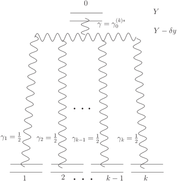
Figure 5: Assuming $\delta y$ is infinitesimal, the anomalous dimensions of $1\Rightarrow k$ amplitude $n_{Y}^{k}$ are illustrated in this figure.

Based on the above computation, one can easily conjecture that the anomalous dimensions of $1\Rightarrow k$ amplitudes should be governed by the equation $k\chi\left(\frac{1}{2}\right)-\chi\left(\gamma\right)=0$, which comes from the dynamical pole introduced by the rapidity integration. Another way of stating this conjecture is that $1\Rightarrow k$ amplitudes tend to have constant energy dependence from $0$ to $Y$(see Fig. 5) as a result of $k\chi\left(\frac{1}{2}\right)=\chi\left(\gamma\right)$. Namely, the total BFKL intercepts of multiple pomeron exchanges are independent of rapidity $y$. Supposing $\gamma_{0}^{\left(k\right)\ast}$ is the solution to this equation between $0$ and $\frac{1}{2}$, then the $1\Rightarrow k$ amplitude should scale as

$$n_{Y\left(q,q_{1}\cdots q_{k}\right)}^{\left(k\right)\left(\rho,\rho_{1}\cdots\rho_{k}\right)} \varpropto \frac{\left(\rho^{2}q^{2}\right)^{1-\gamma_{0}^{\left(k\right)\ast}}}{\left(\rho_{1}q\right)\cdots\left(\rho_{k}q\right)}\frac{\exp\left[k\left(\alpha_{P}-1\right)Y\right]\exp\left[-\frac{\pi\left[\ln^{2}\left(\rho q\right)+\ln^{2}\left(\rho_{1}q_{1}\right)+\cdots+\ln^{2}\left(\rho_{k}q_{k}\right)\right]}{28\alpha C_{F}\zeta\left(3\right)Y}\right]}{\left(7\alpha\zeta\left(3\right)C_{F}Y\right)^{3k/2}}$$ (82)

$$\times\delta^{\left(2\right)}\left(q+q_{1}+\cdots+q_{k}\right)e\left(\rho_{1},q_{1}\right)\cdots e\left(\rho_{k},q_{k}\right).$$

For reader’s convenience, we list the first five $\gamma_{0}^{\left(k\right)\ast}$ in the following: $\gamma_{0}^{\left(1\right)\ast}=\frac{1}{2}$, $\gamma_{0}^{\left(2\right)\ast}=0.18$, $\gamma_{0}^{\left(3\right)\ast}=0.12$, $\gamma_{0}^{\left(4\right)\ast}=0.090$, $\gamma_{0}^{\left(5\right)\ast}=0.072$. This result fits the naive expectation that the anomalous dimension should approach zero in small rapidity limit or in DGLAP limit. Furthermore, when $k$ becomes large enough, we obtain $\gamma_{0}^{\left(k\right)\ast}\simeq 0$. This indicates that the anomalous dimensions of large order pomeron loops are dominated by the DGLAP evolution. We should remind the reader that this conjecture can only be used in the region $\ln^{2}\left(q\rho\right)\ll\frac{14\alpha C_{F}\zeta\left(3\right)}{\pi}Y$ and $\rho^{2}q^{2}\ll 1$, while $q,q_{1}\cdots,q_{k}$ are all of the same order, and so are all the dipole sizes $\rho,\rho_{1}\cdots,\rho_{k}$. In the case of onium-onium scattering, we obtain that the corresponding k-pomeron exchange amplitude should scale as

$$F^{\left(k\right)}\left(\rho,\rho^{\prime},q,Y\right)\propto\left(q^{2}\rho^{2}\right)^{1-\gamma_{0}^{\left(k\right)\ast}}\left(q^{2}\rho^{\prime 2}\right)^{1-\gamma_{0}^{\left(k\right)\ast}}\left\{\alpha^{2}\frac{\exp\left[\left(\alpha_{P}-1\right)Y\right]}{\left(7\alpha\zeta\left(3\right)C_{F}Y\right)^{3/2}}\right\}^{k},$$ (83)

where we restrict ourselves to the $\rho^{2}q^{2}\ll 1$ and $\rho^{\prime 2}q^{2}\ll 1$ limit. As a result, different order of pomeron-loop amplitudes have different dipole size dependence, namely, they belong to different universality classes. Thus, it seems that re-summation of leading order amplitudes is insufficient and impossible to reach unitarity. The argument is straightforward: supposing that unitarity is achieved by resummation of all loop amplitudes by means of delicate balances for fixed $\rho$, it seems impossible to obtain unitarity again when $\rho$ is changed to another value since the delicate balance is then broken.

In summary, according to the conjectured formula, we have found infinite number of new anomalous dimensions between $\frac{1}{2}$ and $0$. Comparing the multiple pomeron exchanges to single pomeron exchange, it seems that the evolution gets pushed towards DGLAP evolutionGribov:1972ri , and the anomalous dimension discretely approaches the anomalous dimension of DGLAP evolution. Because of the lack of the rapidity space for upper and lower pomerons, the evolutions in pomeron loops manage to balance themselves in between the BFKL evolution and the DGLAP evolution. This explains why the new anomalous dimensions are distributed in between $\frac{1}{2}$ and $0$. Furthermore, it is intuitive to notice that the saturation anomalous dimension found in ref. Mueller:2002zm is $\gamma_{s}=0.37$ as a solution to Kovchegov equation in geometric scaling region. Kovchegov equation essentially resums multiple pomeron exchanges (fan diagrams) and yields an anomalous dimension between $\frac{1}{2}$ and $0$ as a result of re-summation of multiple pomeron exchanges. The explicit connection between the $\gamma_{s}$ and $\gamma_{0}^{\left(k\right)\ast}$, however, is still unknown and remains as an open question.

VI Comparison with reggeon field theory calculus

Reggeon field theory (RFT) calculus(for a review, see ref. Baker:1976cv ; Collins:1977jy ; Forshaw:1997dc ; Donnachie:2002en ), similar as Feynman rules, provides definite intercepts ($\alpha\left(t\right)-1=\alpha\left(0\right)+\alpha^{\prime}t$) and propagators for reggeons (including pomerons) in QCD phenomenology. In RFT, the pomeron anomalous dimension $\gamma=\frac{1}{2}$ is a universal (conserved) quantity and it corresponds to the pomeron intercept $\alpha_{P}-1=\frac{8\alpha C_{F}\ln 2}{\pi}$. In leading order of $1\Rightarrow 2$ amplitude, RFT has a genuine triple pomeron vertex which connects 3 pomerons with anomalous dimension $\gamma=\frac{1}{2}$. This approach certainly is justified in some situations such as large diffractive mass scattering, where the large diffractive mass is large enough to fix the anomalous dimension of upper pomeron at $\frac{1}{2}$ by saddle point approximation(e.g., see ref. Bialas:1997xp ). On the other hand, as far as the unitarity problem is concerned, one has to integrate the intermediate rapidity to the upper limit $Y$, in which case the anomalous dimension of the upper pomeron in the vertex is no longer fixed at $\frac{1}{2}$.

Following this philosophy and the essence of the RFT, in order to compare with the calculation we have finished above, let us re-consider $n_{Y}^{(2)}$ in forward scattering ($Q=0,q_{a}=-q_{b}=q$) by assuming that $Y-y$ is always large enough to justify the saddle point approximation (In fact, this assumption breaks down when one integrates rapidity to the upper limit $Y$.) First of all, let us begin with the expression with the rapidity integration,

$$n_{Y,Q,q_{-},0}^{(2)\rho,\rho_{a},\rho_{b}} = \frac{1}{\rho_{a}^{2}\rho_{b}^{2}}\int_{0}^{Y}\frac{\alpha N_{c}}{\pi}dy\mathop{\displaystyle\int}dh\exp\left[\omega\left(\gamma\right)\left(Y-y\right)\right]$$ (84)

$$\times\frac{b_{n,\nu}\left|\rho\right|}{2\pi^{2}}E_{0}^{n,\nu}\left(\rho\right)g_{3P}\left(1-h,\frac{1}{2},\frac{1}{2}\right)4\pi^{2}\left(\frac{4}{q^{2}}\right)^{\gamma-1}\frac{\Gamma^{3}\left(\gamma\right)\Gamma\left(1-2\gamma\right)}{\Gamma\left(2\gamma\right)\Gamma^{3}\left(1-\gamma\right)}$$

$$\times\frac{1}{4\pi^{2}}\frac{\rho_{a}\rho_{b}}{q^{2}}e\left(\rho_{a},q\right)e\left(\rho_{b},-q\right)\frac{\exp\left[2\left(\alpha_{P}-1\right)y\right]\exp\left[-\frac{\pi\left(\ln^{2}\left(q\rho_{a}\right)+\ln^{2}\left(q\rho_{b}\right)\right)}{28\alpha C_{F}\zeta\left(3\right)y}\right]}{\left(7\alpha\zeta\left(3\right)C_{F}y\right)^{3}}$$

Dropping all the higher $n$, and changing $\mathop{\displaystyle\int}dh$ into $\mathop{\displaystyle\int}\frac{d\gamma}{2\pi i}$, one can simplify $n_{Y}^{(2)}$ and get,

$$n_{y,Y,Q,q_{-},0}^{(2)\rho,\rho_{a},\rho_{b}} \simeq \mathop{\displaystyle\int}\frac{d\gamma}{2\pi i}\left(\frac{q^{2}\rho^{2}}{4}\right)^{1-\gamma}\exp\left[\omega\left(\gamma\right)\left(Y-y\right)\right]\frac{4\Gamma\left(\gamma\right)}{\Gamma\left(1-\gamma\right)}g_{3P}\left(1-\gamma,\frac{1}{2},\frac{1}{2}\right)$$ (85)

$$\times\frac{1}{4\pi^{2}}\frac{1}{q^{2}\rho_{a}\rho_{b}}e\left(\rho_{a},q\right)e\left(\rho_{b},-q\right)\frac{\exp\left[2\left(\alpha_{P}-1\right)y\right]\exp\left[-\frac{\pi\left(\ln^{2}\left(q\rho_{a}\right)+\ln^{2}\left(q\rho_{b}\right)\right)}{28\alpha C_{F}\zeta\left(3\right)y}\right]}{\left(7\alpha\zeta\left(3\right)C_{F}y\right)^{3}}$$

If one uses saddle point approximation to evaluate the $\mathop{\displaystyle\int}\frac{d\gamma}{2\pi i}$ integral before the rapidity integral, one reaches,

$$n_{y,Y,Q,q_{-},0}^{(2)\rho,\rho_{a},\rho_{b}} \simeq \frac{1}{8\pi^{2}}\frac{q\rho}{q\rho_{a}q\rho_{b}}g_{3P}\left(\frac{1}{2},\frac{1}{2},\frac{1}{2}\right)e\left(\rho_{a},q\right)e\left(\rho_{b},-q\right)$$ (86)

$$\times\frac{\exp\left[2\left(\alpha_{P}-1\right)y+\left(\alpha_{P}-1\right)\left(Y-y\right)\right]\exp\left[-\frac{\pi\left(\ln^{2}\left(q\rho_{a}\right)+\ln^{2}\left(q\rho_{b}\right)\right)}{28\alpha C_{F}\zeta\left(3\right)y}-\frac{\pi\left(\ln^{2}\left(q\rho\right)\right)}{28\alpha C_{F}\zeta\left(3\right)\left(Y-y\right)}\right]}{\left(7\alpha\zeta\left(3\right)C_{F}y\right)^{3}\left[7\alpha\zeta\left(3\right)C_{F}\left(Y-y\right)\right]^{1/2}}$$

Indeed, we now obtain the genuine triple pomeron vertex which connects 3 pomerons with anomalous dimension $\gamma=\frac{1}{2}$. Finishing the rapidity integration yields,

$$n_{Y,Q,q_{-},0}^{(2)\rho,\rho_{a},\rho_{b}} \simeq \frac{1}{8\pi^{2}}\frac{q\rho}{q\rho_{a}q\rho_{b}}g_{3P}\left(\frac{1}{2},\frac{1}{2},\frac{1}{2}\right)e\left(\rho_{a},q\right)e\left(\rho_{b},-q\right)$$ (88)

$$\times\sqrt{\frac{1}{14\zeta\left(3\right)\ln 2}}\frac{\exp\left[2\left(\alpha_{P}-1\right)Y\right]\exp\left[-\frac{\pi\left(\ln^{2}\left(q\rho_{a}\right)+\ln^{2}\left(q\rho_{b}\right)\right)}{28\alpha C_{F}\zeta\left(3\right)Y}\right]}{\left(7\alpha\zeta\left(3\right)C_{F}Y\right)^{3}}$$

This result agrees with eq.(56) in ref.Mueller:1994jq . Integrating the triple pomeron vertex found in eq.(56) in ref.Mueller:1994jq , one gets

$$\int_{0}^{Y}d\overline{y}\overline{n}_{2}\left(Y,\overline{y},x_{01},q\right) = \int_{0}^{Y}d\overline{y}\frac{\alpha C_{F}V_{0}x_{01}\exp\left[2\left(\alpha_{P}-1\right)\overline{y}+\left(\alpha_{P}-1\right)\left(Y-\overline{y}\right)\right]}{8q\sqrt{7\alpha\zeta\left(3\right)C_{F}\left(Y-\overline{y}\right)}\left(7\alpha\zeta\left(3\right)C_{F}\overline{y}\right)^{3}}$$ (89)

$$\simeq \frac{\pi V_{0}\exp\left[2\left(\alpha_{P}-1\right)Y\right]}{16\sqrt{14\zeta\left(3\right)\ln 2}\left(7\alpha\zeta\left(3\right)C_{F}Y\right)^{3}}\frac{x_{01}}{q}$$ (90)

It clearly differs from Eq.(47) which is proportional to $\frac{\left(\rho^{2}q_{-}^{2}\right)^{1-\gamma_{0}^{\left(2\right)\ast}}}{\rho_{a}q_{-}\rho_{b}q_{-}}g_{3P}\left(0.82,\frac{1}{2},\frac{1}{2}\right)$ as a result of the anomalous dimension being $1-\gamma_{0}^{\left(2\right)\ast}$. The origin of this difference comes from the rapidity integral which dynamically changes the anomalous dimension from $\frac{1}{2}$ to $\gamma_{0}^{\left(2\right)\ast}$.

The zero transverse dimension toy modelsRembiesa:2005gj ; Shoshi:2005pf ; Shoshi:2006eb ; Bondarenko:2006rh ; Kozlov:2006zj ; Blaizot:2006wp , which catch the essence of reggeon field theory calculus, also have universal rules for the pomeron intercepts and propagators, as well as the triple pomeron (or reggeon) vertices. The toy model does not contain the anomalous dimension or transverse dimensions. In some sense, it over-simplifies the problem and fails to catch new features of the QCD pomeron that we found above.

On the other hand, the QCD dipole model, as one can easily spot from the calculation in Sections II, III and IV, contains the distinct feature of the non-existence of universal intercepts and anomalous dimensions for QCD pomerons in the unitarity calculation. In leading order calculation of $1\Rightarrow k$ amplitude, we always push the rapidity integral to the upper limit $Y$ which leaves infinitesimal rapidity for the upper pomeron (see Fig. 5). As a result, the anomalous dimensions of this pomeron are then fixed by the dynamical pole introduced by the rapidity integration. The anomalous dimensions are no longer universal and they vary from graph to graph according to the detail structure of the graph and dynamics. Nevertheless, the other side of the coin is that we now have the constant energy dependence (coefficients of the rapidity) from $0$ to $Y$ while this certainly is not true in RFT.

VII Conclusion

We explicitly calculate the anomalous dimensions of the single, double pomeron and triple pomeron exchange amplitudes in QCD dipole model in the leading logarithmic approximation. Other than the usual pomeron anomalous dimension $\frac{1}{2}$, we find $\gamma_{0}^{(2)\ast}=0.18$ and $\gamma_{0}^{(3)\ast}=0.12$ for double and triple pomeron exchange amplitude, respectively. Based on the calculation, the general formula $\gamma_{0}^{(k)\ast}=\chi^{-1}\left(k\chi\left(\frac{1}{2}\right)\right)$ which governs anomalous dimensions of $1\Rightarrow k$ amplitude is conjectured in the region $\ln^{2}\left(q\rho\right)\ll\frac{14\alpha C_{F}\zeta\left(3\right)}{\pi}Y$ and $\rho^{2}q^{2}\ll 1$, where $\rho$ stands for all the dipole sizes and $q$ represents all the momenta scales.

Furthermore, the calculation of forward scattering $n_{Y}^{\left(2\right)}$ in the $n\neq 0$ case shows that contributions of sub-dominant trajectories of the upper pomeron are suppressed by powers of $\rho^{2}q^{2}$ in $\rho^{2}q^{2}\ll 1$ limit. It is our conjecture that sub-dominant trajectories can be neglect in the non-forward scattering case. We utilize this conjecture in the calculation of $n_{Y}^{\left(3\right)}$ and get rid of the contribution from nonzero value of $n_{d}$.

In addition, different pomeron loop amplitudes (leading order) belong to different universality class as a result of different anomalous dimensions. It seems that re-summation of these amplitudes is insufficient and impossible to reach unitarity. One may have to take higher order contributions into account.

Last but not least, in comparison with the reggeon field theory, one finds that there are two differences between this computation and the reggeon field theory although the BFKL characteristic function $\chi\left(\gamma\right)$ is universal. The first one is that the anomalous dimensions are no longer a constant and they vary according to their positions in the graph while $\gamma=\frac{1}{2}$ everywhere in RFT in order to have a fixed pomeron intercept(for small and fixed $t$ value); the second difference is that the QCD dipole model tends to have a constant energy dependence (coefficients of the rapidity) from $0$ to $Y$ while this certainly is not true in RFT. Namely, the total BFKL intercepts of multiple pomeron exchanges are independent of rapidity $y$ in QCD dipole model. The constancy of the energy dependence is equivalent to the general formula $\gamma_{0}^{(k)\ast}=\chi^{-1}\left(k\chi\left(\frac{1}{2}\right)\right)$ and can easily explain its physical meaning.

Appendix A The evaluation of integrals.

In this and the next appendices, we evaluate the following integral,

$$I_{Q,q_{-}}^{h,h_{a},h_{b}}=\mathop{\displaystyle\int}d^{2}vd^{2}w\exp\left(-iQ\cdot\frac{w}{2}+iq_{-}\cdot v\right)\left[v^{-1+i}\left(\frac{w-v}{2}\right)^{-1+j}\left(\frac{w+v}{2}\right)^{-1+k}\right]\left[a.h.\right].$$ (91)

where a.h. stands for the antiholomorphic part of the square-bracket term. First of all, let us perform the Taylor expansion of the $\exp\left(-iQ\frac{w}{2}\right)$, and keep only the first term $1$. We will discuss the results for higher terms in the next appendix. Thus, the above integral becomes,

$$I_{Q,q_{-}}^{h,h_{a},h_{b},0}=\mathop{\displaystyle\int}d^{2}vd^{2}w\exp\left(iq_{-}\cdot v\right)\left[v^{-1+i}\left(\frac{w-v}{2}\right)^{-1+j}\left(\frac{w+v}{2}\right)^{-1+k}\right]\left[a.h.\right].$$ (92)

A.1 The $d^{2}w$ integral

Furthermore, one can decouple Eq.(92) into two 2-dim integrals in which the $d^{2}w$ integral can be reduced to the following integral:

$$I=\mathop{\displaystyle\int}\frac{dzd\overline{z}}{2i}z^{-1+i}\overline{z}^{-1+\overline{i}}\left(1-z\right)^{j-1}\left(1-\overline{z}\right)^{\overline{j}-1},$$ (93)

where $i-\overline{i}$ and $j-\overline{j}$ are integers. The solution to this integral can be found in Dotsenko and Fateev’s paperDotsenko:1984nm in statistical physics. In the following, we carry out the detailed calculationMunier in complex plane.

The first step is to change $z=x+iy,\overline{z}=x-iy$, and then perform a Wick rotation $y\rightarrow i\left(1-2i\epsilon\right)y$, where the $\epsilon$, which is an infinitesimal positive number, makes sure that the singularities are not touched. We obtain,

$$I=i\int_{-\infty}^{+\infty}dx\int_{-\infty}^{+\infty}dy\left(x-y+2i\epsilon y\right)^{i-1}\left(x+y-2i\epsilon y\right)^{\overline{i}-1}\left(1-x+y-2i\epsilon y\right)^{j-1}\left(1-x-y+2i\epsilon y\right)^{\overline{j}-1}.$$ (94)

Next, one can change the variables into $X_{+}=x+y$ and $X_{-}=x-y$ and cast the integral into the form,

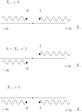
Figure 6: Integral contour of $X_{-}$ and branch cuts in three different domains of $X_{+}$, where the straight line stands for the contour and the photon line represents the branch cuts.

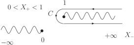
Figure 7: The contour $C$.

$$I = -\frac{i}{2}\int_{-\infty}^{+\infty}dX_{+}\int_{-\infty}^{+\infty}dX_{-}\left[X_{-}+i\epsilon\left(X_{+}-X_{-}\right)\right]^{i-1}\left[X_{+}-i\epsilon\left(X_{+}-X_{-}\right)\right]^{\overline{i}-1}$$ (95)

$$\times\left[1-X_{-}-i\epsilon\left(X_{+}-X_{-}\right)\right]^{j-1}\left[1-X_{+}+i\epsilon\left(X_{+}-X_{-}\right)\right]^{\overline{j}-1}.$$

The integral over $X_{+}$ can be decomposed into 3 pieces with respect to three integration domains(see Fig. 6). Only in the second domain does the integral give non-trivial contribution, since the contour of $X_{-}$ can not be deformed to a single point only in that case. Therefore, we can reach the factorized integrals,

$$I=\int_{0}^{1}dX_{+}X_{+}^{\overline{i}-1}\left(1-X_{+}\right)^{\overline{j}-1}\int_{C}\frac{dX_{-}}{2i}X_{-}^{i-1}\left(1-X_{-}\right)^{j-1},$$ (96)

where contour $C$(see Fig. 7) is a contour which encloses the branch cut $[1,\infty]$. It starts from $i\epsilon+\infty$, goes to $i\epsilon+1$, then crosses the real axis to $-i\epsilon+1$, in the end, goes to $-i\epsilon+\infty$ and forms a close contour. It is straightforward to compute this contour integral and obtain the final result,

$$I = \int_{0}^{1}dX_{+}X_{+}^{\overline{i}-1}\left(1-X_{+}\right)^{\overline{j}-1}$$ (97)

$$\times\left[\exp\left(-i\pi\left(j-1\right)\right)-\exp\left(i\pi\left(j-1\right)\right)\right]\int_{1}^{\infty}\frac{dX_{-}}{2i}X_{-}^{i-1}\left(X_{-}-1\right)^{j-1},$$

$$= \pi\frac{\Gamma\left(\overline{i}\right)\Gamma\left(\overline{j}\right)}{\Gamma\left(\overline{i}+\overline{j}\right)}\frac{\Gamma\left(1-i-j\right)}{\Gamma\left(1-i\right)\Gamma\left(1-j\right)}=\pi\frac{\Gamma\left(i\right)\Gamma\left(j\right)}{\Gamma\left(i+j\right)}\frac{\Gamma\left(1-\overline{i}-\overline{j}\right)}{\Gamma\left(1-\overline{i}\right)\Gamma\left(1-\overline{j}\right)}$$ (98)

Therefore, the $d^{2}w$ integral yields,

$$\mathop{\displaystyle\int}d^{2}w\left[\left(\frac{w-v}{2}\right)^{-1+j}\left(\frac{w+v}{2}\right)^{-1+k}\right]\left[a.h.\right]$$

$$= 4\pi\frac{\Gamma\left(k\right)\Gamma\left(j\right)}{\Gamma\left(k+j\right)}\frac{\Gamma\left(1-\overline{k}-\overline{j}\right)}{\Gamma\left(1-\overline{k}\right)\Gamma\left(1-\overline{j}\right)}v^{j+k-1}\overline{v}^{\overline{j}+\overline{k}-1}.$$

A.2 The $d^{2}v$ integral

The $d^{2}v$ integral can be cast into

$$\mathop{\displaystyle\int}d^{2}v\exp\left(iq_{-}\cdot v\right)v^{\eta-2}\overline{v}^{\overline{\eta}-2},$$ (99)

$$= \int_{0}^{\infty}dr\int_{0}^{2\pi}d\varphi r^{\eta+\overline{\eta}-3}\exp\left[i\left(\eta-\overline{\eta}\right)\varphi+iq_{-}r\cos\varphi\right],$$ (100)

$$= i^{\eta-\overline{\eta}}\pi\left(\frac{2}{q_{-}}\right)^{\eta+\overline{\eta}-2}\frac{\Gamma\left(\eta-1\right)}{\Gamma\left(2-\overline{\eta}\right)},$$ (101)

where $\eta=i+j+k$ and $\eta-\overline{\eta}=-\left(n+n_{a}+n_{b}\,\right)\in Z$. In reaching the above result, we have set the orientation of the $\overrightarrow{q}_{-}$ parallel to the real axis$\left(\varphi_{q_{-}}=0\right)$, and used the following two formulae:

$$J_{m}\left(z\right) = \frac{1}{2\pi i^{m}}\int_{0}^{2\pi}\exp\left(iz\cos\varphi+im\varphi\right),$$ (102)

$$\int_{0}^{\infty}dxx^{\mu}J_{\nu}\left(ax\right) = \frac{2^{\mu}}{a^{\mu+1}}\frac{\Gamma\left(\frac{1}{2}+\frac{\nu}{2}+\frac{\mu}{2}\right)}{\Gamma\left(\frac{1}{2}+\frac{\nu}{2}-\frac{\mu}{2}\right)},$$ (103)

where $m$ should be integers.

Combining the two results, one gets,

$$I_{Q,q_{-}}^{h,h_{a},h_{b},0}=4\pi^{2}i^{-\left(n+n_{a}+n_{b}\,\right)}\left(\frac{4}{q_{-}^{2}}\right)^{\gamma+\gamma_{a}+\gamma_{b}-1}\frac{\Gamma\left(h+h_{a}-h_{b}\right)\Gamma\left(h+h_{b}-h_{a}\right)\Gamma\left(1-2\overline{h}\right)}{\Gamma\left(2h\right)\Gamma\left(1-\overline{h}-\overline{h}_{a}+\overline{h}_{b}\right)\Gamma\left(1-\overline{h}-\overline{h}_{b}+\overline{h}_{a}\right)}\frac{\Gamma\left(h+h_{a}+h_{b}-1\right)}{\Gamma\left(2-\overline{h}-\overline{h}_{a}-\overline{h}_{b}\right)}.$$ (104)

Appendix B Other terms in the Taylor expansion

In this part, we discuss cases of the higher terms of the Taylor series of $\exp\left(iQ\frac{w}{2}\right)$.

B.1 The second term in the expansion

The relevant integral of the second term in the expansion reads,

$$I_{Q,q_{-}}^{h,h_{a},h_{b},1} = \mathop{\displaystyle\int}d^{2}vd^{2}w\exp\left(iq_{-}\cdot v\right)\left[v^{-1+i}\left(\frac{w-v}{2}\right)^{-1+j}\left(\frac{w+v}{2}\right)^{-1+k}\right]\left[a.h.\right]i\frac{Q}{2}\cdot\left[\left(\frac{w-v}{2}\right)+\left(\frac{w+v}{2}\right)\right]$$ (105)

$$= \mathop{\displaystyle\int}d^{2}v\exp\left(iq_{-}\cdot v\right)\left(i\frac{Q}{2}\cdot v\right)v^{\eta-2}\overline{v}^{\overline{\eta}-2}4\pi\frac{\Gamma\left(k\right)\Gamma\left(j\right)}{\Gamma\left(1+k+j\right)}\frac{\Gamma\left(1-\overline{k}-\overline{j}\right)}{\Gamma\left(1-\overline{k}\right)\Gamma\left(1-\overline{j}\right)}.$$ (106)

where $I_{Q,q_{-}}^{h,h_{a},h_{b},l}$ stands for the relevant integral of the $l+1$ term in the Taylor expansion. Assume $i\frac{Q}{2}\cdot v=i\frac{Q}{2}v\cos\left(\phi+\varphi\right)$, where $\phi$ is the orientation of $\overrightarrow{Q}$ in 2-dim plane. $\phi$ should also be considered as the angle between $\overrightarrow{q}_{-}$ and $\overrightarrow{Q}$. It is straightforward to compute the $v$ integral and obtain

$$I_{Q,q_{-}}^{h,h_{a},h_{b},1} = 4\pi^{2}i^{-\left(n+n_{a}+n_{b}\,\right)}\frac{Q}{2q_{-}}\left(\frac{4}{q_{-}^{2}}\right)^{\gamma+\gamma_{a}+\gamma_{b}-1}\frac{\Gamma\left(k\right)\Gamma\left(j\right)}{\Gamma\left(1+k+j\right)}\frac{\Gamma\left(1-\overline{k}-\overline{j}\right)}{\Gamma\left(1-\overline{k}\right)\Gamma\left(1-\overline{j}\right)}\left(k-j\right)$$ (107)

$$\times\left[\exp\left(-i\phi\right)\frac{\Gamma\left(i+j+k-1\right)}{\Gamma\left(1-\overline{i}-\overline{j}-\overline{k}\right)}-\exp\left(i\phi\right)\frac{\Gamma\left(i+j+k-1\right)}{\Gamma\left(1-\overline{i}-\overline{j}-\overline{k}\right)}\right].$$

Since $k-j=2\left(h_{a}-h_{b}\right)$ and eventually $h_{a}=h_{b}=\frac{1}{2}$, $I_{Q,q_{-}}^{h,h_{a},h_{b},1}$ vanishes in the end. Moreover, it is easy to prove that integrals of all odd power of $Q\frac{w}{2}$ are proportional to $k-j$ and they vanish as well.

B.2 The third term in the expansion

The relevant integral of the third term in the expansion reads,

$$I_{Q,q_{-}}^{h,h_{a},h_{b},2} = \mathop{\displaystyle\int}d^{2}vd^{2}w\exp\left(iq_{-}\cdot v\right)\left[v^{-1+i}\left(\frac{w-v}{2}\right)^{-1+j}\left(\frac{w+v}{2}\right)^{-1+k}\right]\left[a.h.\right]\frac{1}{2}\left(i\frac{Q}{2}\cdot w\right)^{2},$$ (109)

$$= \mathop{\displaystyle\int}d^{2}v\exp\left(iq_{-}\cdot v\right)\frac{1}{2}\left(i\frac{Q}{2}\cdot v\right)^{2}v^{\eta-2}\overline{v}^{\overline{\eta}-2}$$

$$\times 4\pi\frac{\Gamma\left(k\right)\Gamma\left(j\right)}{\Gamma\left(2+k+j\right)}\frac{\Gamma\left(1-\overline{k}-\overline{j}\right)}{\Gamma\left(1-\overline{k}\right)\Gamma\left(1-\overline{j}\right)}\left[\left(k-j\right)^{2}+\left(k+j\right)\right].$$

Dropping the $\left(k-j\right)^{2}$ term and finishing the $\mathop{\displaystyle\int}d^{2}v$ integral, one gets

$$I_{Q,q_{-}}^{h,h_{a},h_{b},2} = -4\pi^{2}i^{-\left(n+n_{a}+n_{b}\,\right)}\frac{Q^{2}}{4q_{-}^{2}}\left(\frac{4}{q_{-}^{2}}\right)^{\gamma+\gamma_{a}+\gamma_{b}-1}\frac{\Gamma\left(k\right)\Gamma\left(j\right)}{\Gamma\left(2+k+j\right)}\frac{\Gamma\left(1-\overline{k}-\overline{j}\right)}{\Gamma\left(1-\overline{k}\right)\Gamma\left(1-\overline{j}\right)}\left(k+j\right)$$ (110)

$$\times\left[\frac{\Gamma\left(\eta\right)}{\Gamma\left(1-\overline{\eta}\right)}-\frac{\exp\left(2i\phi\right)}{2}\frac{\Gamma\left(\eta+1\right)}{\Gamma\left(2-\overline{\eta}\right)}-\frac{\exp\left(-2i\phi\right)}{2}\frac{\Gamma\left(\eta-1\right)}{\Gamma\left(-\overline{\eta}\right)}\right].$$

Thus, it is straightforward to examine the singularity structure of $n_{Y,Q,q_{-},2}^{(2)\rho,\rho_{a},\rho_{b}}$(it is proportional to $I_{Q,q_{-}}^{h,h_{a},h_{b},2}$ which comes from the third term in the expansion) before the final $\gamma$ integral in the complex $\gamma$ plane when $n=0$.

$$n_{Y,Q,q_{-},2}^{(2)\rho,\rho_{a},\rho_{b}} \propto \int\frac{d\gamma}{2\pi i}2\pi\frac{2\nu^{2}}{\pi^{4}}\frac{\left|\rho\right|}{2\chi\left(\frac{1}{2}\right)-\chi\left(\gamma\right)}E_{Q}^{0,\nu}\left(\rho\right)g_{3P}\left(1-\gamma,\frac{1}{2},\frac{1}{2}\right)I_{Q,q_{-}}^{h,h_{a},h_{b},2}$$ (111)

$$\propto \int\frac{d\gamma}{2\pi i}\frac{\left|\rho\right|}{2\chi\left(\frac{1}{2}\right)-\chi\left(\gamma\right)}E_{Q}^{0,\nu}\left(\rho\right)g_{3P}\left(1-\gamma,\frac{1}{2},\frac{1}{2}\right)\frac{1}{\gamma+\frac{1}{2}}\left[\frac{\Gamma\left(\gamma+1\right)}{\Gamma\left(-\gamma\right)}-\cos 2\phi\frac{\Gamma\left(\gamma+2\right)}{\Gamma\left(1-\gamma\right)}\right].$$

In addition, one can also show that the fifth term in the expansion

$$n_{Y,Q,q_{-},4}^{(2)\rho,\rho_{a},\rho_{b}} \propto \int\frac{d\gamma}{2\pi i}2\pi\frac{2\nu^{2}}{\pi^{4}}\frac{\left|\rho\right|}{2\chi\left(\frac{1}{2}\right)-\chi\left(\gamma\right)}E_{Q}^{0,\nu}\left(\rho\right)g_{3P}\left(1-\gamma,\frac{1}{2},\frac{1}{2}\right)I_{Q,q_{-}}^{h,h_{a},h_{b},4}$$ (112)

$$\propto \int\frac{d\gamma}{2\pi i}\frac{\left|\rho\right|}{2\chi\left(\frac{1}{2}\right)-\chi\left(\gamma\right)}E_{Q}^{0,\nu}\left(\rho\right)g_{3P}\left(1-\gamma,\frac{1}{2},\frac{1}{2}\right)\frac{1}{\left(\gamma+\frac{1}{2}\right)\left(\gamma+\frac{3}{2}\right)}f_{4}\left[\gamma,\phi\right],$$

where $f_{4}\left[\gamma,\phi\right]$ are terms which are singular only at integer values of $\gamma$. Therefore, we can see the pattern and conclude that $\gamma=0.18$ and $0.82$ are the only two singularities in the $\left(0,1\right)$ domain when $n=0$. In the case when $n\neq 0$, since things are much more complicated, we have been unable to reach similar conclusion. Therefore, we have to restrict ourselves to the forward scattering case in which $Q=0$. Nevertheless, contributions from sub-dominant trajectories would not play any role when one averages over the orientation of the initial onium, since those contributions are all angular dependent and vanish after averaging over angles.

Appendix C Saddle point evaluation of the pomeron

In this appendix, we use saddle point approximation to evaluate the pomeron trajectory when $Y$ is large. The relevant integral is

$$\mathop{\displaystyle\int}dh_{a}\frac{b_{n_{a},\nu_{a}}\left|\rho_{a}\right|}{2\pi^{2}}E_{q_{a}}^{n_{a},\nu_{a}}\left(\rho_{a}\right)\left(\frac{4}{q^{2}}\right)^{\gamma_{a}}\exp\left[\omega\left(a\right)Y\right],$$ (113)

$$\simeq \mathop{\displaystyle\int}_{-\infty}^{+\infty}\frac{d\nu_{a}}{\pi^{4}}2\nu_{a}^{2}\int d^{2}R\exp\left(iq_{a}\cdot R\right)\left(\frac{2\rho_{a}}{\left|R-\frac{\rho_{a}}{2}\right|\left|R+\frac{\rho_{a}}{2}\right|q}\right)^{1+2i\nu_{a}}\exp\left[\omega\left(a\right)Y\right],$$ (114)

$$\simeq \int d^{2}R\frac{\exp\left(iq_{a}\cdot R\right)2\rho_{a}}{\left|R-\frac{\rho_{a}}{2}\right|\left|R+\frac{\rho_{a}}{2}\right|q}\mathop{\displaystyle\int}_{-\infty}^{+\infty}\frac{d\nu_{a}}{\pi^{4}}2\nu_{a}^{2}\exp\left[2\ln 2\overline{\alpha}_{s}Y-7\xi\left(3\right)\nu_{a}^{2}\overline{\alpha}_{s}Y+2i\nu_{a}\ln\frac{2\rho_{a}}{\left|R-\frac{\rho_{a}}{2}\right|\left|R+\frac{\rho_{a}}{2}\right|q}\right],$$ (115)

where $\overline{\alpha}_{s}=\frac{4\alpha_{s}C_{F}}{\pi}$. In reaching the above result, we have used the idea of saddle point approximation and neglected all sub-dominant trajectories. In the region where the diffusion approximation $\ln^{2}\left(q\rho\right)\ll\frac{14\alpha C_{F}\zeta\left(3\right)}{\pi}Y$ is valid, this integral yields

$$\frac{1}{2\pi}\frac{\rho_{a}}{q}e\left(\rho_{a},q_{a}\right)\frac{\exp\left[\left(\alpha_{P}-1\right)Y\right]\exp\left[-\frac{\pi\ln^{2}\left(\rho_{a}q_{a}\right)}{28\alpha C_{F}\zeta\left(3\right)Y}\right]}{\left(7\alpha\zeta\left(3\right)C_{F}Y\right)^{3/2}},$$ (116)

where we have set $\ln^{2}\frac{2\rho_{a}}{\left|R-\frac{\rho_{a}}{2}\right|\left|R+\frac{\rho_{a}}{2}\right|q}\simeq\ln^{2}\left(\rho_{a}q_{a}\right)$ since $\int d^{2}R$ is dominated in the region where $R\sim 1/q_{a}$, and we have defined $e\left(\rho_{a},q_{a}\right)=\frac{1}{2\pi}\int d^{2}R\exp\left(iq_{a}R\right)\frac{1}{\left|R-\frac{\rho_{a}}{2}\right|\left|R+\frac{\rho_{a}}{2}\right|}$, $\alpha_{P}-1=\frac{8\ln 2\alpha_{s}C_{F}}{\pi}$.

Appendix D Explicit calculation of $V_{\nu}$

According to Eq.(50) and Mellin transform, one can easily obtain,

$$\int_{\frac{1}{2}-i\infty}^{\frac{1}{2}+i\infty}\frac{d\gamma}{2\pi i}\left(q^{2}x_{01}^{2}\right)^{\gamma-1}V_{\gamma}=\int\frac{d^{2}x_{2}}{x_{01}x_{12}}J_{0}\left(\frac{1}{2}qx_{01}\right)e\left(x_{12},q\right)e\left(x_{02},q\right).$$ (117)

Evaluating the above integral in $q^{2}x_{01}^{2}\ll 1$ limit, we should close the contour to the right half plane. The leading order term tells us the position of the first pole of $V_{\gamma}$ in complex $\gamma$ plane.

First of all, it is straight forward to discover that

$$e\left(x,q\right)=\frac{1}{\pi}\int_{0}^{1}du\frac{\exp\left[iq\cdot x\left(\frac{1}{2}-u\right)\right]}{\left[u\left(1-u\right)\right]^{1/2}}K_{0}\left[qx\sqrt{u\left(1-u\right)}\right],$$ (118)

where we have used the formulae

$$\frac{1}{\sqrt{ab}}=\frac{1}{\Gamma^{2}\left(\frac{1}{2}\right)}\int_{0}^{1}du\frac{1}{\left[u\left(1-u\right)\right]^{1/2}}\frac{1}{au+b\left(1-u\right)},$$ (119)

and

$$\int_{0}^{\infty}\frac{J_{\nu}\left(qx\right)x^{\nu+1}}{\left(x^{2}+a^{2}\right)^{\mu+1}}dx=\frac{a^{\nu-\mu}q^{\mu}K_{\nu-\mu}\left(qa\right)}{2^{\mu}\Gamma\left(\mu+1\right)}.$$ (120)

Changing variable $u=\sin^{2}\frac{t}{2}$, and combining

$$K_{\mu}\left(x\right) = \frac{\pi}{2\sin\pi\mu}\left[I_{-\mu}\left(x\right)-I_{\mu}\left(x\right)\right],$$ (121)

$$I_{\mu}\left(x\right) = \exp\left(-i\frac{\pi}{2}\mu\right)J_{\mu}\left[\exp\left(-i\frac{\pi}{2}\right)x\right]$$ (122)

along with the integration identity

$$\int_{0}^{\pi/2}J_{\mu}\left[z\sin t\right]\cos\left(x\cos t\right)dt=\frac{\pi}{2}J_{\frac{\mu}{2}}\left[y_{+}\right]J_{\frac{\mu}{2}}\left[y_{-}\right],$$ (123)

where $y_{\pm}=\frac{\sqrt{x^{2}+z^{2}}\pm x}{2}$, gives

$$e\left(x,q\right) = \lim_{\mu\rightarrow 0}\frac{\pi}{2\sin\pi\mu}\left[J_{-\frac{\mu}{2}}\left(\varrho\right)J_{-\frac{\mu}{2}}\left(\varrho^{\ast}\right)-J_{\frac{\mu}{2}}\left(\varrho\right)J_{\frac{\mu}{2}}\left(\varrho^{\ast}\right)\right],$$ (124)

$$= -\frac{\pi}{4}\left[Y_{0}\left(\varrho\right)J_{0}\left(\varrho^{\ast}\right)+J_{0}\left(\varrho\right)Y_{0}\left(\varrho^{\ast}\right)\right],$$ (125)

where $\varrho=\frac{qx}{4}e^{i\psi}$ with $\psi$ being the angle between $\overrightarrow{q}$ and $\overrightarrow{x}$. Therefore,

$$\int\frac{d^{2}x_{2}}{x_{01}x_{12}}J_{0}\left(\frac{1}{2}qx_{01}\right)e\left(x_{12},q\right)e\left(x_{02},q\right)$$ (126)

$$= \frac{\pi^{3}}{8}J_{0}\left(\frac{qx_{10}}{2}\right)\int dx_{12}dx_{20}dbbJ_{0}\left(bx_{01}\right)J_{0}\left(bx_{02}\right)J_{0}\left(bx_{12}\right)$$

$$\times\left[Y_{0}\left(\varrho_{12}\right)J_{0}\left(\varrho_{12}^{\ast}\right)+J_{0}\left(\varrho_{12}\right)Y_{0}\left(\varrho_{12}^{\ast}\right)\right]\left[Y_{0}\left(\varrho_{20}\right)J_{0}\left(\varrho_{20}^{\ast}\right)+J_{0}\left(\varrho_{20}\right)Y_{0}\left(\varrho_{20}^{\ast}\right)\right],$$

where the identitiesMueller:1993rr

$$d^{2}x_{2}=J\left(x_{21},x_{20}\right)dx_{21}dx_{20}=\frac{4x_{21}x_{20}}{\sqrt{\left[\left(x_{21}+x_{20}\right)^{2}-x_{10}^{2}\right]\left[x_{10}^{2}-\left(x_{21}-x_{20}\right)^{2}\right]}},$$ (127)

and

$$\frac{\pi}{2}\int dbbJ_{0}\left(bx_{01}\right)J_{0}\left(bx_{02}\right)J_{0}\left(bx_{12}\right)=\frac{1}{\sqrt{\left[\left(x_{21}+x_{20}\right)^{2}-x_{10}^{2}\right]\left[x_{10}^{2}-\left(x_{21}-x_{20}\right)^{2}\right]}}$$ (128)

have been used. It is easy to estimate the above integral and obtain $\int\frac{d^{2}x_{2}}{x_{01}x_{12}}J_{0}\left(\frac{1}{2}qx_{01}\right)e\left(x_{12},q\right)e\left(x_{02},q\right)\sim\ln\frac{1}{q^{2}x_{10}^{2}}$, which indicates that the first pole of $V_{\gamma}$ occurs at $\gamma=1$.

Appendix E Detailed calculation for higher pomeron trajectories.

Here we consider the integrand of $\int d\gamma$ in the case of general value of $n$,

$$Integrand = 2\pi\frac{2\left(\nu^{2}+n^{4}/4\right)}{\pi^{4}}b_{n,\nu}I_{Q,q_{-}}^{h,h_{a},h_{b},0}$$ (130)

$$= \frac{4\left(\nu^{2}+n^{4}/4\right)}{\pi^{3}}\frac{\pi^{3}2^{4i\nu}}{\left|n\right|/2-i\nu}\frac{\Gamma\left(\left|n\right|/2-i\nu+1/2\right)\Gamma\left(\left|n\right|/2+i\nu\right)}{\Gamma\left(\left|n\right|/2+i\nu+1/2\right)\Gamma\left(\left|n\right|/2-i\nu\right)}$$

$$\times 4\pi^{2}i^{-n}\left(\frac{4}{q^{2}}\right)^{\gamma}\frac{\Gamma^{3}\left(h\right)\Gamma\left(1-2\overline{h}\right)}{\Gamma\left(2h\right)\Gamma^{3}\left(1-\overline{h}\right)}$$

When $n>0$, the integrand yields $\left(-i\right)^{-\left|n\right|}8\pi^{2}\left(\frac{4}{q^{2}}\right)^{\gamma}\frac{\Gamma\left(\gamma+\frac{\left|n\right|}{2}\right)}{\Gamma\left(1+\frac{\left|n\right|}{2}-\gamma\right)}$; when $n<0$, it gives $i^{\left|n\right|}8\pi^{2}\left(\frac{4}{q^{2}}\right)^{\gamma}\frac{\Gamma\left(\gamma+\frac{\left|n\right|}{2}\right)}{\Gamma\left(1+\frac{\left|n\right|}{2}-\gamma\right)}$. Generally, it can be cast into $i^{\left|n\right|}8\pi^{2}\left(\frac{4}{q^{2}}\right)^{\gamma}\frac{\Gamma\left(\gamma+\frac{\left|n\right|}{2}\right)}{\Gamma\left(1+\frac{\left|n\right|}{2}-\gamma\right)}$.

Appendix F Triple pomeron coefficient $g_{3P}$

In this appendix, following KorchemskyKorchemsky:1997fy , we discuss the triple pomeron coefficient $g_{3P}$.

$$g_{3P}\left(h,h_{a},h_{b}\right) = \mathop{\displaystyle\int}\frac{d^{2}\rho_{2}d^{2}\rho_{3}d^{2}\rho_{4}}{\left|\rho_{23}\rho_{34}\rho_{42}\right|^{2}}\rho_{23}^{h}\overline{\rho}_{23}^{\overline{h}}\left(\frac{\rho_{24}}{\rho_{2}\rho_{4}}\right)^{h_{a}}\left(\frac{\overline{\rho}_{24}}{\overline{\rho}_{2}\overline{\rho}_{4}}\right)^{\overline{h}_{a}}$$ (131)

$$\times\left(\frac{\rho_{34}}{\left(1-\rho_{3}\right)\left(1-\rho_{4}\right)}\right)^{h_{b}}\left(\frac{\overline{\rho}_{34}}{\left(1-\overline{\rho}_{3}\right)\left(1-\overline{\rho}_{4}\right)}\right)^{\overline{h}_{b}}$$

Changing the variables: $\rho^{\prime}=\overline{\rho}$ and $\overline{\rho}^{\prime}=\rho$,

$$g_{3P}\left(h,h_{a},h_{b}\right) = \mathop{\displaystyle\int}\frac{d^{2}\rho_{2}^{\prime}d^{2}\rho_{3}^{\prime}d^{2}\rho_{4}^{\prime}}{\left|\rho_{23}^{\prime}\rho_{34}^{\prime}\rho_{42}^{\prime}\right|^{2}}\overline{\rho}_{23}^{\prime h}\rho_{23}^{\prime\overline{h}}\left(\frac{\overline{\rho}_{24}^{\prime}}{\overline{\rho}_{2}^{\prime}\overline{\rho}_{4}}\right)^{h_{a}}\left(\frac{\rho_{24}^{\prime}}{\rho_{2}^{\prime}\rho_{4}^{\prime}}\right)^{\overline{h}_{a}}$$ (132)

$$\times\left(\frac{\overline{\rho}_{34}^{\prime}}{\left(1-\overline{\rho}_{3}^{\prime}\right)\left(1-\overline{\rho}_{4}^{\prime}\right)}\right)^{h_{b}}\left(\frac{\rho_{34}^{\prime}}{\left(1-\rho_{3}^{\prime}\right)\left(1-\rho_{4}^{\prime}\right)}\right)^{\overline{h}_{b}}$$

$$= g_{3P}\left(\overline{h},\overline{h}_{a},\overline{h}_{b}\right),$$ (133)

which means triple pomeron coefficient $g_{3P}$ is an even function of $n$, $n_{a}$ and $n_{b}$. Following the methods used in ref.Korchemsky:1997fy (here our $h$ corresponds the $h_{\gamma}$ in ref.Korchemsky:1997fy ), we find that

$$g_{3P}\left(h,\frac{1}{2},\frac{1}{2}\right)=\frac{1}{\Gamma\left(1-h\right)}\sum_{c=1}^{3}J_{c}\left(h,\frac{1}{2},\frac{1}{2}\right)\overline{J}_{c}\left(\overline{h},\frac{1}{2},\frac{1}{2}\right)$$ (134)

where $J_{c}\left(h,\frac{1}{2},\frac{1}{2}\right)$ and $\overline{J}_{c}\left(\overline{h},\frac{1}{2},\frac{1}{2}\right)$ can be written in terms of Meijer’ G functions $G_{44}^{24}$ and hypergeometric functions $\left.{}_{4}F_{3}\right.$ as follows

$$J_{1}\left(h,\frac{1}{2},\frac{1}{2}\right)=\Gamma\left(1-h\right)G_{44}^{42}\left(1\QATOPD|.{1,\frac{1}{2}+h,1,\frac{3}{2}-h}{\frac{1}{2},\frac{1}{2},\frac{1}{2},\frac{1}{2}}\right)=\Gamma\left(1-h\right)G_{44}^{24}\left(1\QATOPD|.{\frac{1}{2},\frac{1}{2},\frac{1}{2},\frac{1}{2}}{0,\frac{1}{2}-h,0,h-\frac{1}{2}}\right);$$ (135)

$$J_{2}\left(h,\frac{1}{2},\frac{1}{2}\right)=J_{3}\left(h,\frac{1}{2},\frac{1}{2}\right)=\frac{\pi^{2}\Gamma^{3}\left(1-h\right)}{\Gamma\left(\frac{3}{2}-h\right)\Gamma\left(\frac{3}{2}-h\right)}\left.{}_{4}F_{3}\right.\left(\QATOPD.|{\frac{1}{2},\frac{1}{2},1-h,1-h}{1,\frac{3}{2}-h,\frac{3}{2}-h}1\right);$$ (136)

$$J_{3}\left(h,h_{a},h_{b}\right)=J_{2}\left(h,h_{b},h_{a}\right);$$ (137)

$$\overline{J}_{1}\left(\overline{h},\frac{1}{2},\frac{1}{2}\right)=\frac{\pi 2^{-\overline{h}}}{\Gamma\left(1-\overline{h}\right)\Gamma\left(\overline{h}\right)}G_{44}^{42}\left(1\QATOPD|.{1,\frac{3}{2}-\overline{h},1,1}{\frac{1}{2},\frac{1}{2},\frac{1}{2}-\frac{1}{2}\overline{h},1-\frac{1}{2}\overline{h}}\right)=\frac{\pi 2^{-\overline{h}}}{\Gamma\left(1-\overline{h}\right)\Gamma\left(\overline{h}\right)}G_{44}^{24}\left(1\QATOPD|.{\frac{1}{2},\frac{1}{2},\frac{1}{2}\overline{h}+\frac{1}{2},\frac{1}{2}\overline{h}}{0,\overline{h}-\frac{1}{2},0,0}\right);$$ (138)

$$\overline{J}_{2}\left(\overline{h},\frac{1}{2},\frac{1}{2}\right)=\overline{J}_{3}\left(\overline{h},\frac{1}{2},\frac{1}{2}\right)=G_{44}^{42}\left(1\QATOPD|.{1,\frac{3}{2}-\overline{h},1,\frac{1}{2}+\overline{h}}{\frac{1}{2},\frac{1}{2},\frac{1}{2},\frac{1}{2}}\right)=G_{44}^{24}\left(1\QATOPD|.{\frac{1}{2},\frac{1}{2},\frac{1}{2},\frac{1}{2}}{0,\overline{h}-\frac{1}{2},0,\frac{1}{2}-\overline{h}}\right);$$ (139)

$$\overline{J}_{3}\left(\overline{h},\overline{h}_{a},\overline{h}_{b}\right)=\overline{J}_{2}\left(\overline{h},\overline{h}_{b},\overline{h}_{a}\right).$$ (140)

We find different but equivalent final expressions of $J_{c}\left(h,h_{a},h_{b}\right)$ and $\overline{J}_{c}\left(\overline{h},\overline{h}_{a},\overline{h}_{b}\right)$ as compared to those in ref.Korchemsky:1997fy . Numerically, one finds $g_{3P}\left(\frac{1}{2},\frac{1}{2},\frac{1}{2}\right)=7766.68$ which agrees with the previous result in ref.Korchemsky:1997fy ; Bialas:1997ig . Thus, we outline our evaluation of the $g_{3P}\left(h,\frac{1}{2},\frac{1}{2}\right)$ in the following. For instance, from ref.Korchemsky:1997fy , one can get

$$\overline{J}_{1}\left(\overline{h},\frac{1}{2},\frac{1}{2}\right)=\frac{\pi^{3}}{\Gamma\left(1-\overline{h}\right)\Gamma\left(\overline{h}\right)}\int_{0}^{1}dxx^{-\overline{h}}\left(1-x\right)^{-1+\overline{h}}\left.{}_{2}F_{1}\right.\left(\QATOPD.|{\frac{1}{2},\frac{1}{2}}{1}x\right)\left.{}_{2}F_{1}\right.\left(\QATOPD.|{\frac{1}{2},\frac{1}{2}}{1}x\right).$$ (141)

Using the identityBialas:1997ig

$$\left.{}_{2}F_{1}\right.\left(\QATOPD.|{\frac{1}{2},\frac{1}{2}}{1}x\right)\left.{}_{2}F_{1}\right.\left(\QATOPD.|{\frac{1}{2},\frac{1}{2}}{1}x\right)=\frac{1}{\left(1-x\right)^{1/2}}\left.{}_{3}F_{2}\right.\left(\QATOPD.|{\frac{1}{2},\frac{1}{2},\frac{1}{2}}{1,1}-\frac{x^{2}}{4\left(1-x\right)}\right),$$ (142)

and the Mellin-Barnes representation of hypergeometric function

$$\left.{}_{3}F_{2}\right.\left(\QATOPD.|{\frac{1}{2},\frac{1}{2},\frac{1}{2}}{1,1}z\right)=\frac{1}{\Gamma^{3}\left(\frac{1}{2}\right)}\int_{-i\infty}^{+i\infty}\frac{ds}{2\pi i}\frac{\Gamma^{3}\left(\frac{1}{2}+s\right)\Gamma\left(-s\right)}{\Gamma^{2}\left(1+s\right)}\left(-z\right)^{s},$$ (143)

along with identities

$$\int_{0}^{1}dxx^{\mu-1}\left(1-x\right)^{\nu-1} = \frac{\Gamma\left(\mu\right)\Gamma\left(\nu\right)}{\Gamma\left(\mu+\nu\right)},$$ (144)

$$\Gamma\left(2s\right) = \frac{2^{2s-1}}{\sqrt{\pi}}\Gamma\left(s\right)\Gamma\left(s+\frac{1}{2}\right),$$ (145)

one obtains,

$$\overline{J}_{1}\left(\overline{h},\frac{1}{2},\frac{1}{2}\right) = \frac{\pi 2^{-\overline{h}}}{\Gamma\left(1-\overline{h}\right)\Gamma\left(\overline{h}\right)}$$ (146)

$$\times\int_{-i\infty}^{+i\infty}\frac{ds}{2\pi i}\frac{\Gamma^{2}\left(\frac{1}{2}+s\right)\Gamma\left(s+\frac{1}{2}-\frac{1}{2}\overline{h}\right)\Gamma\left(s+1-\frac{1}{2}\overline{h}\right)\Gamma\left(-s\right)\Gamma\left(\overline{h}-\frac{1}{2}-s\right)}{\Gamma^{2}\left(1+s\right)}.$$

According to the definition of the Meijer’s G function

$$G_{pq}^{mn}\left(z\QATOPD|.{a_{1},\ldots,a_{p}}{b_{1},\ldots,b_{q}}\right)=\int_{-i\infty}^{+i\infty}\frac{ds}{2\pi i}\frac{\mathop{\displaystyle\prod}\limits_{j=1}^{m}\Gamma\left(b_{j}+s\right)\mathop{\displaystyle\prod}\limits_{j=1}^{n}\Gamma\left(1-a_{j}-s\right)}{\mathop{\displaystyle\prod}\limits_{j=m+1}^{q}\Gamma\left(1-b_{j}-s\right)\mathop{\displaystyle\prod}\limits_{j=n+1}^{p}\Gamma\left(a_{j}+s\right)}z^{-s},$$ (147)

one can easily reach the expression we found above. It is straightforward to put $g_{3P}\left(h,\frac{1}{2},\frac{1}{2}\right)$ into Mathematica and plot it for fixed integer values of $n$ as function of $\gamma$. The plots for the first few integer values of $n$ show that $g_{3P}\left(h,\frac{1}{2},\frac{1}{2}\right)$ has no pole in the domain $\left(-\frac{\left|n\right|}{2},\frac{\left|n\right|}{2}+1\right)$.

References

- (1) I. I. Balitsky and L. N. Lipatov, Sov. J. Nucl. Phys. 28, 822 (1978) [Yad. Fiz. 28, 1597 (1978)].
- (2) E. A. Kuraev, L. N. Lipatov and V. S. Fadin, Sov. Phys. JETP 45, 199 (1977) [Zh. Eksp. Teor. Fiz. 72, 377 (1977)].
- (3) L. N. Lipatov, Sov. Phys. JETP 63, 904 (1986) [Zh. Eksp. Teor. Fiz. 90, 1536 (1986)].
- (4) A. H. Mueller, Nucl. Phys. B 415, 373 (1994);
- (5) A. H. Mueller and B. Patel, Nucl. Phys. B 425, 471 (1994).
- (6) A. H. Mueller, Nucl. Phys. B 437 (1995) 107;
- (7) H. Navelet and S. Wallon, Nucl. Phys. B 522, 237 (1998)
- (8) Y. V. Kovchegov, Phys. Rev. D 60, 034008 (1999).
- (9) A. H. Mueller and A. I. Shoshi, Nucl. Phys. B 692 (2004) 175.
- (10) E. Iancu, A. H. Mueller and S. Munier, Phys. Lett. B 606 (2005) 342.
- (11) S. Munier and R. Peschanski, Phys. Rev. Lett. 91 (2003) 232001; S. Munier and R. Peschanski, Phys. Rev. D 69 (2004) 034008.
- (12) E. Iancu and D. N. Triantafyllopoulos, Nucl. Phys. A 756 (2005) 419.
- (13) A. H. Mueller, A. I. Shoshi and S. M. H. Wong, Nucl. Phys. B 715 (2005) 440.
- (14) E. Iancu and D. N. Triantafyllopoulos, Phys. Lett. B 610 (2005) 253.
- (15) A. Kovner and M. Lublinsky, Phys. Rev. D 71 (2005) 085004.
- (16) Y. Hatta, E. Iancu, L. McLerran, A. Stasto and D. N. Triantafyllopoulos, Nucl. Phys. A 764, 423 (2006).
- (17) A. Kovner and M. Lublinsky, Phys. Rev. Lett. 94 (2005) 181603; A. Kovner and M. Lublinsky, JHEP 0503 (2005) 001; A. Kovner and M. Lublinsky, Phys. Rev. D 72 (2005) 074023; A. Kovner and M. Lublinsky, Nucl. Phys. A 767, 171 (2006).
-
(18)
J. P. Blaizot, E. Iancu, K. Itakura and
D. N. Triantafyllopoulos,
Phys. Lett. B 615 (2005) 221.
Y. Hatta, E. Iancu, L. McLerran and A. Stasto, Nucl. Phys. A 762 (2005) 272.
E. Iancu, G. Soyez and D. N. Triantafyllopoulos, Nucl. Phys. A 768, 194 (2006). - (19) C. Marquet, A. H. Mueller, A. I. Shoshi and S. M. H. Wong, Nucl. Phys. A 762 (2005) 252.
- (20) E. Levin and M. Lublinsky, Nucl. Phys. A 763, 172 (2005); E. Levin, Nucl. Phys. A 763, 140 (2005).
- (21) R. Enberg, K. Golec-Biernat and S. Munier, Phys. Rev. D 72 (2005) 074021.
- (22) G. Soyez, Phys. Rev. D 72, 016007 (2005); C. Marquet, G. Soyez and B. W. Xiao, Phys. Lett. B 639, 635 (2006).
- (23) Y. Hatta, E. Iancu, C. Marquet, G. Soyez and D. N. Triantafyllopoulos, Nucl. Phys. A 773, 95 (2006).
- (24) E. Iancu, C. Marquet and G. Soyez, Nucl. Phys. A 780, 52 (2006).
- (25) M. Kozlov, A. I. Shoshi and B. W. Xiao, Nucl. Phys. A 792, 170 (2007).
- (26) M. Kozlov, A. Shoshi and W. Xiang, JHEP 0710, 020 (2007).
- (27) H. Navelet and R. Peschanski, Nucl. Phys. B 634, 291 (2002).
- (28) R. Peschanski, Phys. Lett. B 409, 491 (1997).
- (29) M. A. Braun and G. P. Vacca, Eur. Phys. J. C 6, 147 (1999).
- (30) Y. Hatta and A. H. Mueller, Nucl. Phys. A 789, 285 (2007).
- (31) G. P. Korchemsky, Nucl. Phys. B 550, 397 (1999).
- (32) E. Levin, J. Miller and A. Prygarin, arXiv:0706.2944 [hep-ph].
- (33) H. Navelet and R. Peschanski, Nucl. Phys. B 507, 353 (1997).
- (34) V. N. Gribov and L. N. Lipatov, Sov. J. Nucl. Phys. 15, 438 (1972) [Yad. Fiz. 15, 781 (1972)]. G. Altarelli and G. Parisi, Nucl. Phys. B 126, 298 (1977). Y. L. Dokshitzer, Sov. Phys. JETP 46 (1977) 641 [Zh. Eksp. Teor. Fiz. 73 (1977) 1216].
- (35) G. P. Salam, Acta Phys. Polon. B 30, 3679 (1999).
- (36) A. H. Mueller, arXiv:hep-ph/9911289.
- (37) R. A. Janik and R. Peschanski, Nucl. Phys. B 549, 280 (1999).
- (38) A. H. Mueller and D. N. Triantafyllopoulos, Nucl. Phys. B 640, 331 (2002).
- (39) M. Baker and K. A. Ter-Martirosian, Phys. Rept. 28, 1 (1976).
- (40) P. D. B. Collins, “An Introduction To Regge Theory And High-Energy Physics,” Cambridge 1977, 445p; P. D. B. Collins, Phys. Rept. 1, 103 (1971).
- (41) J. R. Forshaw and D. A. Ross, Cambridge Lect. Notes Phys. 9, 1 (1997).
- (42) S. Donnachie, H. G. Dosch, O. Nachtmann and P. Landshoff, Camb. Monogr. Part. Phys. Nucl. Phys. Cosmol. 19, 1 (2002).
- (43) A. Bialas, H. Navelet and R. Peschanski, Phys. Lett. B 427, 147 (1998).
- (44) P. Rembiesa and A. M. Stasto, Nucl. Phys. B 725, 251 (2005).
- (45) A. I. Shoshi and B. W. Xiao, Phys. Rev. D 73, 094014 (2006).
- (46) A. I. Shoshi and B. W. Xiao, Phys. Rev. D 75, 054002 (2007).
- (47) S. Bondarenko, L. Motyka, A. H. Mueller, A. I. Shoshi and B. W. Xiao, Eur. Phys. J. C 50, 593 (2007).
- (48) M. Kozlov and E. Levin, Nucl. Phys. A 779, 142 (2006).
- (49) J. P. Blaizot, E. Iancu and D. N. Triantafyllopoulos, Nucl. Phys. A 784, 227 (2007).
- (50) V. S. Dotsenko and V. A. Fateev, Nucl. Phys. B 240, 312 (1984); V. S. Dotsenko and V. A. Fateev, Nucl. Phys. B 251, 691 (1985).
- (51) Private communication with Stephane Munier. I would like to thank Stephane Munier for the notes about the computation of some integrals.
- (52) A. Bialas, H. Navelet and R. Peschanski, Phys. Rev. D 57, 6585 (1998); L.J.Slater, “Generalized hypergeometric functions”, Cambridge University Press (1966).