Increasing power of the test through pre-test
- a robust method

Abstract

This paper develops robust test procedures for testing the intercept of a simple regression model when it is apriori suspected that the slope has a specified value. Defining unrestricted test (UT), restricted test (RT) and pre-test test (PTT) corresponding to the unrestricted (UE), restricted (RE), and preliminary test estimators (PTE) in the estimation case, the M-estimation methodology is used to formulate the M-tests and derive their asymptotic power functions. Analytical and graphical comparisons of the three tests are obtained by studying the power functions with respect to size and power of the tests. It is shown that PTT achieves a reasonable dominance over the others asymptotically.

Keywords: pre-test, asymptotic size, asymptotic power, M-estimation, contiguity, regression model.

1 Introduction

In recent years many researchers have contributed to the estimation of one parameter in the presence of uncertain prior information on the value of another parameter. In general, inclusion of non-sample prior information improves the quality of inference. In spite of plethora of work in the area of improved estimation using non-sample prior information (c.f. Saleh, 2006), very little attention has been paid on the testing of parameters in the presence of uncertain prior information. It may be a normal expectation that testing of one parameter after pre-testing on another would improve the performance of the ultimate test in the sense of better power and size of the ultimate test. In this paper, this improvement is achieved by using a robust test, namely score type M-test defined along the line of M-estimation methodology.

If the underlying distribution is known and the assumed model holds, the statistical test that offers the most powerful test is the classical likelihood ratio test (LRT). However, this parametric test is generally very non-robust, even to small departures from the assumed distribution (c.f. Huber, 1981, p.264, Jur$\check{e}$ckov$\acute{a}$ and Sen, 1996, p.408). Several robust tests are suggested in literature to tackle the problem. For example, Huber (1981, p.264) suggests some censored likelihood ratio type test and shows the test possesses a minimax property. The test however does not work out conveniently for composite null hypothesis against composite alternative testing problem (c.f. Jur$\check{e}$ckov$\acute{a}$ and Sen 1996 p.407). The Rao’s efficient score statistic could be tempted on the least favorable distribution to obtain a robust test statistic. Sen (1982) suggests a score type statistic by replacing the robust Rao score test statistic by an M-statistic. The score-type M-test has several advantages. The construction of the score-type M-test needs less parameters to estimate than the robust LRT suggested by Schrader and Hettmansperger (1980) yet both are equiefficient (c.f. Sen, 1982) and are applicable to composite hypothesis testing.

The properties of unrestricted estimator (UE), restricted estimator (RE) and pre-test estimator (PTE) have been investigated by many authors (Khan and Saleh, 2001, Khan et al., 2002). Most of the studies are based on normal or t-models and the results are non-robust. In the studies, the PTE (a linear combination of UE and RE) possesses a small quadratic risk when the distance parameter are large and too close to zero, that makes it the best choice over the other two estimators. Instead of least squares (LS) and maximum likelihood (ML) estimators, the properties of UE, RE and PTE are also studied in the framework of general robust estimators, explicitly, M-estimators. As such, a robust estimator namely the preliminary test M-estimator (PTME) are proposed for linear models (Sen and Saleh, 1987). In this paper, three tests correspond to the UE, RE and PTE are defined. They are unrestricted test (UT), restricted test (RT) and pre-test test (PTT). The study of the properties on these tests formulated using robust statistics is unavailable in the statistics literature.

The properties of size of the pre-test as well as the power of the test followed by pre-test have been studied in parametric cases (Bechhofer, 1951, Bozivich et al., 1956). After almost three decades, the effect of pre-test (on slope) on the size and power of the ultimate test (on the intercept) are investigated for rank-based nonparametric cases by Saleh and Sen (1982). However, there are some limited discussions in investigating the power of the PTT discussed in the paper. To author’s knowledge, no research has been done in the investigation of the performance (size and power) of the ultimate test following a pre-test in linear models that is formulated using the score-type M-test. Since the M-estimation method is more popular compared to the other robust methods, it is incomplete to ignore the study of the performance characteristics of the power function after pre-testing based on M-test. M-estimation is known for its flexibility and well defined for a variety of models for which MLE is also defined (Huber, 1981, p.43, Jur$\check{e}$ckov$\acute{a}$ and Sen, 1996 p.80). In this paper, the study on the power of test after pre-testing using M-test is considered for a simple linear regression model.

Consider a simple regression model of $n$ observable random variables, $X_{i},\;i=1,\ldots,n$

$$X_{i}=\theta+\beta c_{i}+e_{i},$$ (1.1)

where the errors $e_{i}$’s are from an unspecified symmetric and continuous distribution function, $F_{i},\;i=1,\ldots,n,$ the $c_{i}$’s are known real constants of the explanatory variable and $\theta$ and $\beta$ are the unknown intercept and slope parameters respectively.

We wish to test the significance of the intercept parameter under various conditions on the slope parameter. Basically, testing the intercept of a simple linear regression depends on the knowledge on the slope. We may have the case when the slope is unspecified. For this case, the slope is treated as a nuisance parameter in testing the significance of the intercept and we refer the test as the unrestricted test (UT). We may also have the case when the value of the slope is specified (say zero) and thus we return to the situation of testing the location parameter. The test on the intercept after specifying the value of slope is defined as the restricted test (RT). Besides these two cases, if the value of the slope is suspected to be close to 0 (or any specified value), a natural action is to remove the uncertainty of the suspicious value of the slope by performing a test on the slope before testing the intercept. If the null hypothesis of the pre-test is rejected, then we use the UT, otherwise the RT. This is in line with definition of the PTE in the estimation problem. For the final case, the ultimate test following a pre-test is defined as the pre-test test (PTT). Obviously the preliminary test (on the slope) affects the power and size of the ultimate test (on the intercept). To simplify,

• The unrestricted test : Test function $\phi_{n}^{UT}$ is designed for testing $H_{0}^{\star}:\theta=0$ when $\beta$ is unspecified,

• The restricted test: The test function $\phi_{n}^{RT}$ is designed for testing $H_{0}^{\star}:\theta=0$ when $\beta$ is 0 (specified) and

• The pre-test test : The test function $\phi_{n}^{PTT}$ is designed for testing $H_{0}^{\star}:\theta=0$ following a pre-test on the slope.

The objectives of the current research are to propose a robust test statistic based on M-statistic to formulate the asymptotic power functions for testing the intercept after pre-testing on slope and to carry out investigations on the asymptotic properties of this power function.

Along with some preliminary notions, the method of M-estimation is presented in Section 2. In Section 3, three statistical tests concerning testing on the intercept, namely, the UT, RT and PTT are proposed for the three different cases mention earlier. Further, the asymptotic distributions of the test statistics are derived in Section 4. In Section 5, the asymptotic power functions of the tests are derived. Section 6 is devoted to the analytical results comparing the asymptotic power functions of the UT, RT and PTT while the investigation of the power functions through an illustrative example is presented in Section 7. The final section presents discussions and concluding remarks.

2 The M-estimation

Given an absolutely continuous function $\rho:\Re\rightarrow\Re$, M-estimator of $\theta$ and $\beta$ is defined as the values of $\theta$ and $\beta$ that minimize the objective function

$$\sum_{i=1}^{n}\rho(X_{i}-\theta-\beta c_{i}).$$ (2.1)

M-estimator of $\theta$ and $\beta$ can also be defined as the solutions of the system of equations,

$$\begin{array}[]{ccccc}\sum_{i=1}^{n}\psi_{\theta}(X_{i})&=&\sum_{i=1}^{n}\psi(X_{i}-\theta-\beta c_{i})&=&0,\\ \sum_{i=1}^{n}\psi_{\beta}(X_{i})&=&\sum_{i=1}^{n}c_{i}\psi(X_{i}-\theta-\beta c_{i})&=&0.\end{array}$$ (2.2)

If $\rho$ is differentiable with partial derivatives $\psi_{\theta}=\partial{\rho}/\partial{\theta}$ and $\psi_{\beta}=\partial{\rho}/\partial{\beta}$, then the M-estimators that minimize the function in (2.1) are the solutions to the system (2.2). On the contrary, the M-estimators obtained from solving system (2.2) may not minimize equation (2.1) (c.f. Caroll and Rupert, 1988 p.210). The system of equations (2.2) may have more roots, while only one of them leads to a global minimum of (2.1). Jur$\check{e}$ckov$\acute{a}$ and Sen (1996) have given proof that there exists at least one root of (2.2) which is a $\sqrt{n}$ - consistent estimator of $\theta$ and $\beta$ under some conditions [c.f. p.215 - 224]. The $\psi$ function is decomposed into the sum

$$\psi=\psi_{a}+\psi_{c}+\psi_{s},$$

where

(a) $\psi_{a}$ is absolutely continuous function with absolutely continuous derivative.

(b) $\psi_{c}$ is a continuous, piecewise linear function with knots at $\mu_{1},\ldots,\mu_{k}$, that is, constant in a neighborhood of $\pm\infty$ and hence its derivative is a step function $\psi_{c}^{\prime}(z)=\alpha_{v},\;\mu_{v}<z<\mu_{v+1},\;v=0,1,\ldots,k$ where $\alpha_{0},\ldots,\alpha_{k}\;\epsilon\;\Re,\;\alpha_{0}=\alpha_{k}=0$ and $-\infty=\mu_{0}<\mu_{1}<\ldots<\mu_{k+1}=\infty$. We assume that $f(z)=\frac{dF(z)}{dz}$ is bounded in neighborhoods of $S_{\mu_{1}},\ldots,S_{\mu_{k}}.$

(c) $\psi_{s}$ is a nondecreasing step function, $\psi_{s}(z)=\lambda_{v},\;q_{v}<z\leq q_{v+1},v=1,\ldots,m$ where $-\infty=q_{0}<q_{1}<\ldots<q_{m+1}=\infty$ and $-\infty<\lambda_{0}<\lambda_{1}<\ldots<\lambda_{m}<\infty.$ We assume that $0<f(z)=(d/dz)F(z)$ and $f^{\prime}(z)=(d^{2}/dz^{2})F(z)$ are bounded in neighborhoods of $S_{q_{1}},\ldots,S_{q_{m}}.$

The asymptotic result under conditions M1 to M5 of Jur$\check{e}$ckov$\acute{a}$ and Sen (1996, p.217) is used in this paper. Further assume that all $\psi_{a}$, $\psi_{c}$ and $\psi_{s}$ are nondecreasing and skew symmetric that is $\psi_{j}(-x)=-\psi_{j}(x),\;j=1,2,3.$ Let $F$ be symmetric about 0, so that

$$\int_{-\infty}^{\infty}\psi(x)dF(x)=0.$$

Assume that

$$\sigma_{0}^{2}=\int_{-\infty}^{\infty}\psi^{2}(x)dF(x).$$ (2.3)

Following Jur$\check{e}$ckov$\acute{a}$ and Sen (1996, p.217), two cases are considered:

(i) if $\psi_{s}=0$ then

$$\gamma=\int_{-\infty}^{\infty}(\psi_{a}^{\prime}(x)+\psi_{c}^{\prime}(x))f(x)dx.$$ (2.4)

(ii) if $\psi_{a}=\psi_{c}=0$, then

$$\gamma=\sum(\lambda_{v}-\lambda_{v-1})f(S_{q_{v}}).$$ (2.5)

Further assume that $\sigma_{0}$ and $\gamma$ are both positive and finite quantities. Let the distribution function, $F$ be continuous and symmetric about zero and have finite Fisher information,

$$I(f)=\int_{-\infty}^{\infty}\{f^{\prime}(x)/f(x)\}^{2}dF(x),$$ (2.6)

where $f^{\prime}(x)=(d/dx)f(x)=(d^{2}/dx^{2})F(x).$ Assume that

(i) there exists finite constants $\bar{c}$ and $C^{\star}(>0)$ such that

$$\lim_{n\rightarrow^{\infty}}\bar{c}_{n}=\bar{c}\;\;\;\mbox{and}\;\;\;\lim_{n\rightarrow\infty}n^{-1}{C_{n}^{\star}}^{2}={C^{\star}}^{2}$$ (2.7)

with

$$\bar{c}_{n}=n^{-1}\sum_{i=1}^{n}c_{i}\;\;\;\mbox{and}\;\;\;{C_{n}^{\star}}^{2}=\sum_{i=1}^{n}c_{i}^{2}-n\bar{c}_{n}^{2}$$ (2.8)

both exist.

(ii) the $c_{i}$’s are all bounded, so that by (i),

$$\max_{1\leq i\leq n}(c_{i}-\bar{c}_{n})^{2}/{C_{n}^{\star}}^{2}\rightarrow 0,\;\;\;\mbox{as}\;\;n\rightarrow\infty.$$ (2.9)

Let $\psi:\Re\rightarrow\Re$ be nondecreasing and skew symmetric score function. For any real numbers $a$ and $b$, consider the statistics below

$$M_{n_{1}}(a,b)=\sum_{i=1}^{n}\psi(X_{i}-a-bc_{i}),$$ (2.10)

$$M_{n_{2}}(a,b)=\sum_{i=1}^{n}c_{i}\psi(X_{i}-a-bc_{i}).$$ (2.11)

Let $\tilde{\beta}$ be the constrained M-estimator of $\beta$ when $\theta=0$, that is, $\tilde{\beta}$ is the solution of $M_{n_{2}}(0,b)=0$ and it may be conveniently be expressed as

$$\tilde{\beta}=[\underbrace{\sup\{b:M_{n_{2}}(0,b)>0\}}_{b_{1}}\;+\;\underbrace{\inf\{b:M_{n_{2}}(0,b)<0\}}_{b_{2}}]/2.$$ (2.12)

Any value $b_{1}<b<b_{2}$ can serve as the estimate of $M_{n}(0,b).$ However $\tilde{\beta}$, the centroid (and the median) of the interval $[b_{1},\;b_{2}]$ achieves the smallest maximum bias among all translation invariant functionals (Huber, 1981 p.75), hence it is a robust estimator with optimum robustness properties. Similarly, let $\tilde{\theta}$ be the constrained M-estimator of $\theta$ when $\beta=0$, that is, $\tilde{\theta}$ is the solution of $M_{n_{1}}(a,0)=0$ and conveniently be expressed as

$$\tilde{\theta}=[\sup\{a:M_{n_{1}}(a,0)>0\}\;+\;\inf\{a:M_{n_{1}}(a,0)<0\}]/2.$$ (2.13)

By the same argument as above, $\tilde{\theta}$ is a robust estimator.

The preliminaries notations and assumptions in this section are used to develop the tests and construct the asymptotic power functions of the UT, RT and PTT. In the next section, the UT and RT are proposed. The PT (testing on slope) is introduced and the PTT is constructed.

3 The UT, RT and PTT

Sen (1982) shows that the asymptotic distribution of

$$n^{-1/2}M_{n_{2}}(\tilde{\theta},0)\rightarrow N(0,\sigma_{0}^{2}{C^{\star}}^{2})$$ (3.1)

under $H_{0}^{(1)}:\beta=0.$ The consistency of $[S_{n}^{(3)}]^{2}=n^{-1}\sum_{i=1}^{n}\psi^{2}(X_{i}-\tilde{\theta})$ as an estimator of $\sigma_{0}^{2}$ follows from Jur$\check{e}$ckov$\acute{a}$ and Sen (1981). Hence, a test statistic $A_{n}=M_{n_{2}}(\tilde{\theta},0)[C_{n}^{\star}\;S_{n}^{(3)}]^{-1}$ is proposed by Sen (1982). The advantage of this test statistic (score-type M-test) is that it does not require the computation of the M-estimates or the estimation of functional $\gamma.$

By the same way, it is easy to show that the asymptotic distribution of

$$n^{-1/2}M_{n_{1}}(0,\tilde{\beta})\rightarrow N(0,\sigma_{0}^{2}{C^{\star}}^{2}/\{{C^{\star}}^{2}+\bar{c}^{2}\})$$ (3.2)

under $H_{0}^{\star}:\theta=0.$ By the same token, the consistency of $[S_{n}^{(1)}]^{2}=n^{-1}\sum_{i=1}^{n}\psi^{2}(X_{i}-\tilde{\beta}c_{i})$ as an estimator of $\sigma_{0}^{2}$ follows.

These two asymptotic distributions results are useful to construct suitable test in formulating the asymptotic power function for testing the intercept after pre-testing. We are primarily concerned with statistical tests for the parameter $\theta$ as well as $\beta.$ In essence we need to consider four test functions correspond to the four proposed tests.

3.1 The unrestricted test (UT)

If $\beta$ is unspecified, the designated test function is $\phi_{n}^{UT}$ with the null hypothesis $H_{0}^{\star}:\theta=0$. The testing for $\theta$ involves the elimination of the nuisance parameter $\beta$. It follows that $M_{n_{2}}(0,b)$ is decreasing if $b$ is increasing (Jur$\check{e}$ckov$\acute{a}$ and Sen, 1996, p.85) and under local hypothesis, $H_{0}^{(1)}:\beta=0$, $M_{n_{2}}(0,0)$ has expectation 0. Then let

$$\tilde{\beta}=(\sup\{b:M_{n_{2}}(0,b)>0\}+\inf\{b:M_{n_{2}}(0,b)<0\})/2.$$

Then $\tilde{\beta}$ is a translation invariant and robust estimator of $\beta$.

We consider the test statistic $T_{n}^{UT}=M_{n_{1}}(0,\tilde{\beta})$ where under $H_{0}^{\star}$, as $n\rightarrow\infty,$

$$\frac{T_{n}^{UT}}{\sqrt{C_{n}^{(1)}{S_{n}^{(1)}}^{2}}}\rightarrow N(0,1)$$

with $C_{n}^{(1)}=n-n^{2}\bar{c}_{n}^{2}/\sum c_{i}^{2}=n{C_{n}^{\star}}^{2}/({C_{n}^{\star}}^{2}+n\bar{c}_{n}^{2})$ and $[S_{n}^{(1)}]^{2}=\sum\psi^{2}(x_{i}-\tilde{\beta}c_{i})/n.$

3.2 The restricted test (RT)

If $\beta=0$, the designated test function is $\phi_{n}^{RT}$ for testing the null hypothesis $H_{0}^{\star}:\theta=0$. The proposed test statistic is $T_{n}^{RT}=M_{n_{1}}(0,0).$ Note that for large $n$, under $H_{0}:\theta=0,\beta=0$,

$$n^{-1/2}T_{n}^{RT}=n^{-1/2}M_{n_{1}}(0,0)\rightarrow N(0,\sigma_{0}^{2}),$$ (3.3)

where $\sigma_{0}^{2}=\int_{-\infty}^{\infty}\psi^{2}(x)dF(x)$ (see Sen, 1982, eq 3.7).

3.3 The pre-test test (PTT)

In this section, test on slope is proposed first and followed by the construction of the ultimate test for testing intercept.

For the preliminary test on the slope, the test function, $\phi_{n}^{PT}$ is designed to test the null hypothesis $H_{0}^{(1)}:\beta=0$. The proposed test statistic is $T_{n}^{PT}=M_{n_{2}}(\tilde{\theta},0)$ where

$$\tilde{\theta}=(\sup\{a:M_{n_{1}}(a,0)>0\}+\inf\{a:M_{n_{1}}(a,0)<0\})/2$$

is a robust estimator. Under $H_{0}^{(1)}$, as $n\rightarrow\infty,$

$$\frac{T_{n}^{PT}}{\sqrt{C_{n}^{(3)}{S_{n}^{(3)}}^{2}}}\rightarrow N(0,1),$$

where $C_{n}^{(3)}=\sum c_{i}^{2}-n\bar{c}_{n}^{2}={C_{n}^{\star}}^{2}$ and $[S_{n}^{(3)}]^{2}=\sum\psi^{2}(x_{i}-\tilde{\theta})/n.$

The consistency of $[S_{n}^{(1)}]^{2}$, $[S_{n}^{(2)}]^{2}=\sum\psi^{2}(x)/n$ and $[S_{n}^{(3)}]^{2}$ as estimators of $\sigma_{0}^{2}$ follows by law of large number (Jur$\check{e}$ckov$\acute{a}$ and Sen, 1981).

Now, we are in a position to formulate a test function $\phi_{n}^{PTT}$ to test $H_{0}^{\star}:\theta=0$ following a preliminary test on $\beta.$ First, we consider the case where all of $\phi_{n}^{(j)},\;j=1,2,3$ are one-sided test. Let us choose positive numbers $\alpha_{j}\;(0<\alpha_{j}<1)$ and real values $\ell_{n,\alpha_{j}}^{(j)},\;j=1,2,3,$ such that for large sample size,

$$P[T_{n}^{UT}>\ell_{n,\alpha_{1}}^{UT}|H_{0}^{\star}:\theta=0]=\alpha_{1},$$ (3.4)

$$P[T_{n}^{RT}>\ell_{n,\alpha_{2}}^{RT}|H_{0}:\theta=0,\beta=0]=\alpha_{2},$$ (3.5)

$$P[T_{n}^{PT}>\ell_{n,\alpha_{3}}^{PT}|H_{0}^{(1)}:\beta=0]=\alpha_{3},$$ (3.6)

where $\ell_{n,\alpha_{j}}^{(j)}$ is the critical value of $T_{n}^{(j)}$ at the $\alpha_{j}$ level of significance. Let $\Phi(x)$ be the standard normal cumulative distribution function, then

$$\Phi(\tau_{\alpha})=1-\alpha,\;\;\mbox{for}\;\;0<\alpha<1.$$ (3.7)

Using equations (3.3), (3.5) and (3.7), we obtain

$$\begin{array}[]{rcl}\vspace{10pt}1-\alpha_{2}&=&P[T_{n}^{RT}\leq\ell_{n,\alpha_{2}}^{RT}]\\ &=&\vspace{10pt}P\left[n^{-1/2}T_{n}^{RT}/\sqrt{{S_{n}^{(2)}}^{2}}\leq n^{-1/2}\ell_{n,\alpha_{2}}^{RT}/\sqrt{{S_{n}^{(2)}}^{2}}\;\right]\\ &\rightarrow&P\left[n^{-1/2}T_{n}^{RT}/\sqrt{\sigma_{0}^{2}}\leq n^{-1/2}\ell_{n,\alpha_{2}}^{RT}/\sqrt{\sigma_{0}^{2}}\;\right]=\Phi(n^{-1/2}\ell_{n,\alpha_{2}}^{RT}/\sigma_{0}),\\ \end{array}$$

where ${S_{n}^{(2)}}^{2}=\sum\psi^{2}(x_{i})/n.$ Thus as $n\rightarrow\infty$ we have

$$\frac{n^{-1/2}\ell_{n,\alpha_{2}}^{RT}}{\sqrt{{S_{n}^{(2)}}^{2}}}\rightarrow\tau_{\alpha_{2}}=\frac{n^{-1/2}\ell_{n,\alpha_{2}}^{RT}}{\sqrt{\sigma_{0}^{2}}}\;\;\mbox{(say).}$$ (3.8)

By the same way, using (3.2) and (3.4), we observe that as $n\rightarrow\infty$,

$$\frac{n^{-1/2}\ell_{n,\alpha_{1}}^{UT}}{\sqrt{{S_{n}^{(1)}}^{2}C_{n}^{(1)}/n}}\rightarrow\tau_{\alpha_{1}}=\frac{n^{-1/2}\ell_{n,\alpha_{1}}^{UT}}{\sqrt{\sigma_{0}^{2}{C^{\star}}^{2}/({C^{\star}}^{2}+\bar{c}^{2})}}\;\;\mbox{(say)},$$ (3.9)

where ${S_{n}^{(1)}}^{2}=\sum\psi^{2}(x_{i}-\tilde{\beta}c_{i})/n,$ and $C_{n}^{(1)}=n-n^{2}\bar{c}_{n}^{2}/\sum c_{i}^{2}.$ Also by (3.1) and (3.6), as $n\rightarrow\infty,$

$$\frac{n^{-1/2}\ell_{n,\alpha_{3}}^{PT}}{\sqrt{{S_{n}^{(3)}}^{2}{C_{n}^{\star}}^{2}/n}}\rightarrow\tau_{\alpha_{3}}=\frac{n^{-1/2}\ell_{n,\alpha_{3}}^{PT}}{\sqrt{\sigma_{0}^{2}{C^{\star}}^{2}}}\;\;\mbox{(say),}$$ (3.10)

where ${S_{n}^{(3)}}^{2}=\sum\psi^{2}(x_{i}-\tilde{\theta})/n,$ and ${C_{n}^{\star}}^{2}=\sum c_{i}^{2}-n\bar{c}_{n}^{2}.$

Now we may write

$$\phi_{n}^{PTT}=I\left[(T_{n}^{PT}\leq\ell_{n,\alpha_{3}}^{PT},T_{n}^{RT}>\ell_{n,\alpha_{2}}^{RT})\;\;\mbox{or}\;\;(T_{n}^{PT}>\ell_{n,\alpha_{3}}^{PT},T_{n}^{UT}>\ell_{n,\alpha_{1}}^{UT})\right]$$ (3.11)

as the test function for testing $H_{0}^{\star}:\theta=0$ after a pre-test on $\beta.$ Note that $I(A)$ stands for the indicator function of the set $A.$ It takes value 1 if $A$ occurs, otherwise 0. The function enables us to define the power of the test $\phi_{n}^{PTT}$, that is given by

$$\Pi_{n}^{PTT}(\theta) = E(\phi_{n}^{PTT}|\theta)$$ (3.12)

$$= P[T_{n}^{PT}\leq\ell_{n,\alpha_{3}}^{PT},T_{n}^{RT}>\ell_{n,\alpha_{2}}^{RT}|\theta]+P[T_{n}^{PT}>\ell_{n,\alpha_{3}}^{PT},T_{n}^{UT}>\ell_{n,\alpha_{1}}^{UT}|\theta].$$

In general, the power of the test $\phi_{n}^{PTT}$ depends on $\alpha_{1},\alpha_{2},\alpha_{3},\theta,n$ as well as $\beta.$ Note that the size of the ultimate test $\alpha_{n}^{PTT}$ is a special case of the power of the test when $\theta=0.$ Since the nuisance parameter $\beta$ is unknown, but, suspected to be close to 0, it is of interest to study the dependence of both $\alpha_{n}^{PTT}$ and $\Pi_{n}^{PTT}(\theta)$ on $\beta$ (close to 0).

4 Asymptotic distribution of $T_{n}^{UT}$, $T_{n}^{RT}$ and $T_{n}^{PT}$

This section is devoted to the asymptotic distribution theory of statistics involved in proposing the PTT. The asymptotic joint distributions of $\left[T_{n}^{UT},T_{n}^{PT}\right]$ and $\left[T_{n}^{RT},T_{n}^{PT}\right]$ are derived. The results are used in the next section in the construction of the power function of the UT, RT and PTT.

Let $\{K_{n}\}$ be a sequence of alternative hypotheses, where

$$K_{n}:(\theta,\beta)=(n^{-1/2}\lambda_{1},n^{-1/2}\lambda_{2}),$$ (4.1)

with $\lambda_{1},\lambda_{2}$ are (fixed) real numbers.

Interested readers are referred to Jur$\check{e}$ckov$\acute{a}$ (1977), Sen (1982) and Jur$\check{e}$ckov$\acute{a}$ and Sen (1996, p.221) for the following asymptotic properties:

(i) under $H_{0}:\theta=0,\beta=0,$ as $n$ grows large,

$$n^{-1/2}\left(\begin{array}[]{c}M_{n_{1}}(0,0)\\ M_{n_{2}}(0,0)\end{array}\right)\rightarrow N_{2}\left(\left[\begin{array}[]{c}0\\ 0\end{array}\right],\sigma_{0}^{2}\left(\begin{array}[]{cc}1&\bar{c}\\ \bar{c}&{C^{\star}}^{2}+\bar{c}^{2}\\ \end{array}\right)\right),$$ (4.2)

where $N_{2}(\cdot\;,\cdot\;)$ represents a bivariate normal distribution with appropriate parameters.

(ii) under $H_{0}:\theta=0,\beta=0,$

$$\begin{array}[]{c}\vspace{10pt}\sup\{n^{-1/2}|M_{n_{1}}(a,b)-M_{n_{1}}(0,0)+n\gamma(a+b\bar{c})|:\\ |a|\leq n^{-1/2}K,|b|\leq n^{-1/2}K\}\rightarrow_{p}0\end{array}$$ (4.3)

as $n\rightarrow\infty$ and $K$ is a positive constant.

(iii) under $H_{0}:\theta=0,\beta=0,$

$$\begin{array}[]{c}\vspace{10pt}\sup\{n^{-1/2}|M_{n_{2}}(a,b)-M_{n_{2}}(0,0)+n\gamma\{a\bar{c}+b({C^{\star}}^{2}+\bar{c}^{2})\}|:\\ \hskip 150.0pt|a|\leq n^{-1/2}K,|b|\leq n^{-1/2}K\}\rightarrow_{p}0\end{array}$$ (4.4)

as $n\rightarrow\infty$ and $K$ is a positive constant. The above convergence is in probability, means the sequences of random variables converges in probability to a fix value (0).

An important concept that dominates the asymptotic theory of statistics is the contiguity of probability measures (Jur$\check{e}$ckov$\acute{a}$ and Sen, 1996, p.61). Contiguity arguments are a technique to obtain the limit distribution of a sequence of statistics under the alternative hypothesis from a limiting distribution under the null hypothesis (c.f. van der Vaart, 1998 p.85). Let $\{P_{n}\}$ and $\{Q_{n}\}$ be two sequence of probability measures defined in a measure spaces $(\Omega_{n},B_{n},\mu_{n}).$ In the LeCam’s first lemma (H$\acute{a}$jek et al., 1999, p.251), if

$$\log L_{n}\stackrel{{\scriptstyle D}}{{\rightarrow}}N(-\frac{1}{2}\;\sigma^{2},\sigma^{2})\;\;(\mbox{under}\;\;\{P_{n}\}),$$

then $\{Q_{n}\}$ is contiguous to $\{P_{n}\}.$ Here the likelihood ratio statistic $L_{n}$ is given by

$$L_{n}=\left\{\begin{array}[]{ccc}q_{n}/p_{n}&\mbox{for}&p_{n}>0\\ 1&\mbox{for}&p_{n}=q_{n}=0\\ \infty&\mbox{for}&0=p_{n}<q_{n},\end{array}\right.$$

where $\{p_{n},q_{n}\}$ are the sequence of simple hypothesis densities. In the LeCam’s third lemma (H$\acute{a}$jek et al., 1999, p.257), if

$$\left[\begin{array}[]{c}T_{n}\\ \log L_{n}\end{array}\right]\stackrel{{\scriptstyle D}}{{\rightarrow}}N_{2}\left(\left[\begin{array}[]{c}\mu_{1}\\ \mu_{2}\end{array}\right],\left[\begin{array}[]{cc}\sigma_{11}&\sigma_{12}\\ \sigma_{21}&\sigma_{22}\\ \end{array}\right]\right)\;\;(\mbox{under}\;\;\{P_{n}\}),$$

where $T_{n}$ is a statistic with $\mu_{2}=-\frac{1}{2}\sigma_{22}$, then

$$T_{n}\stackrel{{\scriptstyle D}}{{\rightarrow}}N(\mu_{1}+\sigma_{12},\;\sigma_{11})\;\;(\mbox{under}\;\;\{Q_{n}\}).$$

The LeCam’s second lemma (H$\acute{a}$jek et al., 1999, p.253) gives conditions when $\log L_{n}\stackrel{{\scriptstyle D}}{{\rightarrow}}N(-\frac{1}{2}\;\sigma^{2},\sigma^{2})$.

The concept of contiguity is more popular in R-estimation (rank statistic) than in M-estimation. However, Sen (1982) uses the contiguity of probability measures under $H_{n}:\beta=n^{-1/2}\lambda$ to those under $H_{0}^{\prime}:\beta=0$ to find the asymptotic distribution of $n^{-1/2}\left[M_{n_{1}}(\theta,0),M_{n_{2}}(\theta,0)\right]$ under $H_{n}.$ In this paper, the contiguity concept is utilized to find the asymptotic distributions of statistics $n^{-1/2}[\;T_{n}^{RT},T_{n}^{PT}]$ and $n^{-1/2}[\;T_{n}^{UT},T_{n}^{PT}]$ under $K_{n}.$

4.1 Asymptotic distribution of $n^{-1/2}T_{n}^{RT}$ and $n^{-1/2}T_{n}^{PT}$

Following Jur$\check{e}$ckov$\acute{a}$ and Sen (1996, p.259), let $\{P_{n}\}$ and $\{Q_{n}\}$ denote the probability distributions with the densities $p_{n}=\prod_{i=1}^{n}f(X_{i})$ and $q_{n}=\prod_{i=1}^{n}f(X_{i}-n^{-1/2}\lambda_{1}-tc_{ni})$ of the null hypothesis $H_{0}$ and the alternative hypothesis $K_{n},$ respectively, where $c_{ni}=(c_{i}-\bar{c}_{n})/C_{n}^{\star},\;\;i=1,\ldots,n.$ Note that under (1.1), (2.7), (2.9) and (4.1), the contiguity of the sequence of probability measures under $\{K_{n}\}$ to those under $H_{0}$ follows from LeCam’s first and second lemmas (H$\acute{a}$jek et al., 1999, Chapter 7). We are interested in the asymptotic distribution of the joint statistics $\left[n^{-1/2}T_{n}^{RT},n^{-1/2}T_{n}^{PT}\right].$ Here convergence of $\left[n^{-1/2}T_{n}^{RT},n^{-1/2}T_{n}^{PT}\right]+\Upsilon\rightarrow[0,0]$ under $H_{0}$ implies $\left[n^{-1/2}T_{n}^{RT},n^{-1/2}T_{n}^{PT}\right]+\Upsilon\rightarrow[0,0]$ under $\{K_{n}\}$ since the probability measures under $\{K_{n}\}$ is contiguous to that of under ${H_{0}}$ (c.f. Saleh, 2006, p.44). Here, $\Upsilon$ is a known vector.

Under $H_{0}:\theta=0,\;\beta=0,$ with relation to (4.3) and (4.4),

$$\left[\begin{array}[]{cc}n^{-1/2}M_{n_{1}}(0,0)\\ n^{-1/2}M_{n_{2}}(\tilde{\theta},0)\end{array}\right]-\left[\begin{array}[]{c}n^{-1/2}M_{n_{1}}(0,0)\\ n^{-1/2}M_{n_{2}}(0,0)\\ \end{array}\right]+\left[\begin{array}[]{c}0\\ n^{1/2}\gamma\tilde{\theta}\bar{c}\\ \end{array}\right]\rightarrow_{p}\left[\begin{array}[]{c}0\\ 0\end{array}\right]$$ (4.13)

or equivalently

$$n^{-1/2}M_{n_{1}}(0,0)=n^{-1/2}M_{n_{1}}(0,0)+o_{p}(1)$$ (4.14)

and

$$n^{-1/2}M_{n_{2}}(\tilde{\theta},0)=n^{-1/2}M_{n_{2}}(0,0)-n^{1/2}\gamma\tilde{\theta}\bar{c}+o_{p}(1).$$ (4.15)

Note also that under $H_{0}:\theta=0,\;\beta=0,$

$$n^{-1/2}M_{n_{1}}(\tilde{\theta},0)=n^{-1/2}M_{n_{1}}(0,0)-n^{1/2}\gamma\tilde{\theta}+o_{p}(1).$$ (4.16)

Recalling definition (2.13), the equation (4.16) reduces to

$$n^{-1/2}M_{n_{1}}(0,0)=n^{1/2}\gamma\tilde{\theta}+o_{p}(1),$$ (4.17)

and hence equation (4.15) becomes

$$n^{-1/2}M_{n_{2}}(\tilde{\theta},0)=n^{-1/2}M_{n_{2}}(0,0)-n^{-1/2}M_{n_{1}}(0,0)\bar{c}+o_{p}(1).$$ (4.18)

Therefore, under $H_{0}$, equation (4.13) becomes

$$\vspace{5pt}\left[\begin{array}[]{c}n^{-1/2}M_{n_{1}}(0,0)\\ n^{-1/2}M_{n_{2}}(\tilde{\theta},0)\\ \end{array}\right]-\left[\begin{array}[]{c}n^{-1/2}M_{n_{1}}(0,0)\\ n^{-1/2}M_{n_{2}}(0,0)-n^{-1/2}M_{n_{1}}(0,0)\bar{c}\\ \end{array}\right]\hskip 50.0pt$$ (4.22)

$$\hskip 50.0pt\vspace{5pt}=\left[\begin{array}[]{c}n^{-1/2}M_{n_{1}}(0,0)\\ n^{-1/2}M_{n_{2}}(\tilde{\theta},0)\\ \end{array}\right]-\left[\begin{array}[]{cc}1&0\\ -\bar{c}&1\\ \end{array}\right]\left[\begin{array}[]{c}n^{-1/2}M_{n_{1}}(0,0)\\ n^{-1/2}M_{n_{2}}(0,0)\\ \end{array}\right]\rightarrow_{p}\left[\begin{array}[]{c}0\\ 0\end{array}\right].$$ (4.31)

Now utilizing the contiguity of probability measures under $\{K_{n}\}$ to those under $H_{0}$, the equation (4.31) implies that

$$\left[\begin{array}[]{c}n^{-1/2}M_{n_{1}}(0,0)\\ n^{-1/2}M_{n_{2}}(\tilde{\theta},0)\\ \end{array}\right]$$

under $\{K_{n}\}$ is asymptotically equivalent to the random vector

$$\left[\begin{array}[]{cc}1&0\\ -\bar{c}&1\\ \end{array}\right]\left[\begin{array}[]{c}n^{-1/2}M_{n_{1}}(0,0)\\ n^{-1/2}M_{n_{2}}(0,0)\\ \end{array}\right]$$

under $H_{0}.$ But the asymptotic distribution of the above random vector under $\{K_{n}\}$ is the same as

$$\left[\begin{array}[]{cc}1&0\\ -\bar{c}&1\\ \end{array}\right]\left[\begin{array}[]{c}n^{-1/2}M_{n_{1}}(-n^{-1/2}\lambda_{1},-n^{-1/2}\lambda_{2})\\ n^{-1/2}M_{n_{2}}(-n^{-1/2}\lambda_{1},-n^{-1/2}\lambda_{2})\\ \end{array}\right]$$

under $H_{0}$ by the fact that the distribution of $M_{n_{1}}(a,b)$ under $\theta=a,\beta=b$ is the same as that of $M_{n_{1}}(\theta-a,\beta-b)$ under $\theta=0,\beta=0,$ and similarly for $M_{n_{2}}(0,0)$ (c.f. Saleh, 2006 p.332).

Note that under $H_{0}:\theta=0,\beta=0$, with relation to (4.3) and (4.4),

$$\begin{array}[]{c}\vspace{10pt}\left[\begin{array}[]{cc}n^{-1/2}M_{n_{1}}(-n^{-1/2}\lambda_{1},-n^{-1/2}\lambda_{2})\\ n^{-1/2}M_{n_{2}}(-n^{-1/2}\lambda_{1},-n^{-1/2}\lambda_{2})\end{array}\right]-\left[\begin{array}[]{c}n^{-1/2}M_{n_{1}}(0,0)\\ n^{-1/2}M_{n_{2}}(0,0)\\ \end{array}\right]\\ \hskip 50.0pt-\left[\begin{array}[]{c}\gamma(\lambda_{1}+\lambda_{2}\bar{c})\\ \gamma\{\lambda_{1}\bar{c}+\lambda_{2}({C^{\star}}^{2}+\bar{c}^{2})\}\\ \end{array}\right]\rightarrow_{p}\left[\begin{array}[]{c}0\\ 0\end{array}\right].\end{array}$$ (4.32)

Hence, by equation (4.2), under $H_{0}$,

$$\left[\begin{array}[]{c}n^{-1/2}M_{n_{1}}(-n^{-1/2}\lambda_{1},-n^{-1/2}\lambda_{2})\\ n^{-1/2}M_{n_{2}}(-n^{-1/2}\lambda_{1},-n^{-1/2}\lambda_{2})\\ \end{array}\right]$$ (4.35)

$$\;\;\;\;\;\;\;\;\;\rightarrow N_{2}\left(\left(\begin{array}[]{c}\gamma(\lambda_{1}+\lambda_{2}\bar{c})\\ \gamma\{\lambda_{1}\bar{c}+\lambda_{2}({C^{\star}}^{2}+\bar{c}^{2})\}\\ \end{array}\right),\;\sigma_{0}^{2}\left(\begin{array}[]{cc}1&\bar{c}\\ \bar{c}&{C^{\star}}^{2}+\bar{c}^{2}\\ \end{array}\right)\right).$$ (4.40)

Thus, the distribution of

$$\left[\begin{array}[]{c}n^{-1/2}T_{n}^{RT}\\ n^{-1/2}T_{n}^{PT}\end{array}\right]=\left[\begin{array}[]{c}n^{-1/2}M_{n_{1}}(0,0)\\ n^{-1/2}M_{n_{2}}(\tilde{\theta},0)\\ \end{array}\right]$$

under $\{K_{n}\}$ is bivariate normal with mean vector

$$\left[\begin{array}[]{cc}1&0\\ -\bar{c}&1\\ \end{array}\right]\left[\begin{array}[]{c}\gamma(\lambda_{1}+\lambda_{2}\bar{c})\\ \gamma\{\lambda_{1}\bar{c}+\lambda_{2}({C^{\star}}^{2}+\bar{c}^{2})\}\end{array}\right]=\left[\begin{array}[]{c}\gamma(\lambda_{1}+\lambda_{2}\bar{c})\\ \gamma\lambda_{2}{C^{\star}}^{2}\end{array}\right]$$

and covariance matrix

$$\left[\begin{array}[]{cc}1&0\\ -\bar{c}&1\\ \end{array}\right]\sigma_{0}^{2}\left(\begin{array}[]{cc}1&\bar{c}\\ \bar{c}&{C^{\star}}^{2}+\bar{c}^{2}\\ \end{array}\right)\left[\begin{array}[]{cc}1&0\\ -\bar{c}&1\\ \end{array}\right]^{\prime}=\sigma_{0}^{2}\left[\begin{array}[]{cc}1&0\\ 0&{C^{\star}}^{2}\\ \end{array}\right].$$ (4.41)

Since the two statistics $n^{-1/2}T_{n}^{RT}$ and $n^{-1/2}T_{n}^{PT}$ are uncorrelated, asymptotically, they are independently distributed normal variables.

4.2 Asymptotic distribution of $n^{-1/2}T_{n}^{UT}$ and $n^{-1/2}T_{n}^{PT}$

Under $H_{0}:\theta=0,\beta=0,$ with relation to (4.3) and (4.4), as $n\rightarrow\infty,$

$$\vspace{10pt}\left[\begin{array}[]{cc}n^{-1/2}M_{n_{1}}(0,\tilde{\beta})\\ n^{-1/2}M_{n_{2}}(\tilde{\theta},0)\end{array}\right]-\left[\begin{array}[]{c}n^{-1/2}M_{n_{1}}(0,0)\\ n^{-1/2}M_{n_{2}}(0,0)\\ \end{array}\right]\left[\begin{array}[]{c}n^{1/2}\gamma\tilde{\beta}\bar{c}\\ n^{1/2}\gamma\tilde{\theta}\bar{c}\\ \end{array}\right]\rightarrow_{p}\left[\begin{array}[]{c}0\\ 0\end{array}\right]$$ (4.50)

or equivalently

$$n^{-1/2}M_{n_{1}}(0,\tilde{\beta})=n^{-1/2}M_{n_{1}}(0,0)-n^{1/2}\gamma\tilde{\beta}\bar{c}+o_{p}(1)$$ (4.51)

and

$$n^{-1/2}M_{n_{2}}(\tilde{\theta},0)=n^{-1/2}M_{n_{2}}(0,0)-n^{1/2}\gamma\tilde{\theta}\bar{c}+o_{p}(1).$$ (4.52)

Again under $H_{0}:\theta=0,\beta=0,$

$$n^{-1/2}M_{n_{2}}(0,\tilde{\beta})=n^{-1/2}M_{n_{2}}(0,0)-n^{1/2}\gamma\tilde{\beta}({C^{\star}}^{2}+\bar{c}^{2})+o_{p}(1).$$ (4.53)

But by definition (2.12), we have

$$n^{-1/2}M_{n_{2}}(0,0)=n^{1/2}\gamma\tilde{\beta}({C^{\star}}^{2}+\bar{c}^{2})+o_{p}(1),$$ (4.54)

so equation (4.51) becomes

$$n^{-1/2}M_{n_{1}}(0,\tilde{\beta})=n^{-1/2}M_{n_{1}}(0,0)-n^{-1/2}M_{n_{2}}(0,0)\bar{c}/({C^{\star}}^{2}+\bar{c}^{2})+o_{p}(1).$$ (4.55)

Hence, under $H_{0}$, using equations (4.18) and (4.55), equation (4.50) becomes

$$\vspace{5pt}\left[\begin{array}[]{c}n^{-1/2}M_{n_{1}}(0,\tilde{\beta})\\ n^{-1/2}M_{n_{2}}(\tilde{\theta},0)\\ \end{array}\right]-\left[\begin{array}[]{c}n^{-1/2}M_{n_{1}}(0,0)-n^{-1/2}M_{n_{2}}(0,0)\bar{c}/({C^{\star}}^{2}+\bar{c}^{2})\\ n^{-1/2}M_{n_{2}}(0,0)-n^{-1/2}M_{n_{1}}(0,0)\bar{c}\\ \end{array}\right]\hskip 50.0pt$$ (4.60)

$$\hskip 1.0pt\vspace{5pt}=\left[\begin{array}[]{c}n^{-1/2}M_{n_{1}}(0,\tilde{\beta})\\ n^{-1/2}M_{n_{2}}(\tilde{\theta},0)\\ \end{array}\right]-\left[\begin{array}[]{cc}1&-\bar{c}/({C^{\star}}^{2}+\bar{c}^{2})\\ -\bar{c}&1\\ \end{array}\right]\left[\begin{array}[]{c}n^{-1/2}M_{n_{1}}(0,0)\\ n^{-1/2}M_{n_{2}}(0,0)\\ \end{array}\right]\rightarrow_{p}\left[\begin{array}[]{c}0\\ 0\end{array}\right].$$ (4.69)

Now by using the contiguity of probability measures under $\{K_{n}\}$ to those under ${H_{0}}$, the equation (4.69) implies that

$$\left[\begin{array}[]{c}n^{-1/2}M_{n_{1}}(0,\tilde{\beta})\\ n^{-1/2}M_{n_{2}}(\tilde{\theta},0)\\ \end{array}\right]$$

under $\{K_{n}\}$ is asymptotically equivalent to the random vector

$$\left[\begin{array}[]{cc}1&-\bar{c}/({C^{\star}}^{2}+\bar{c}^{2})\\ -\bar{c}&1\\ \end{array}\right]\left[\begin{array}[]{c}n^{-1/2}M_{n_{1}}(0,0)\\ n^{-1/2}M_{n_{2}}(0,0)\\ \end{array}\right].$$

But the asymptotic distribution of the above random vector under $\{K_{n}\}$ is the same as

$$\left[\begin{array}[]{cc}1&-\bar{c}/({C^{\star}}^{2}+\bar{c}^{2})\\ -\bar{c}&1\\ \end{array}\right]\left[\begin{array}[]{c}n^{-1/2}M_{n_{1}}(-n^{-1/2}\lambda_{1},-n^{-1/2}\lambda_{2})\\ n^{-1/2}M_{n_{2}}(-n^{-1/2}\lambda_{1},-n^{-1/2}\lambda_{2})\\ \end{array}\right]$$

under $H_{0}$ by the fact that the distribution of $M_{n_{1}}(a,b)$ under $\theta=a,\beta=b$ is the same as that of $M_{n_{1}}(\theta-a,\beta-b)$ under $\theta=0,\beta=0$ and similarly for $M_{n_{2}}(0,0)$ (c.f. Saleh, 2006 p.332).

Then it follows that by equation (4.40),

$$\left[\begin{array}[]{c}n^{-1/2}T_{n}^{UT}\\ n^{-1/2}T_{n}^{PT}\end{array}\right]=\left[\begin{array}[]{c}n^{-1/2}M_{n_{1}}(0,\tilde{\beta})\\ n^{-1/2}M_{n_{2}}(\tilde{\theta},0)\\ \end{array}\right]$$

is bivariate normal with mean vector

$$\left[\begin{array}[]{cc}1&-\bar{c}/({C^{\star}}^{2}+\bar{c}^{2})\\ -\bar{c}&1\\ \end{array}\right]\left[\begin{array}[]{c}\gamma(\lambda_{1}+\lambda_{2}\bar{c})\\ \gamma\{\lambda_{1}\bar{c}+\lambda_{2}({C^{\star}}^{2}+\bar{c}^{2})\}\end{array}\right]=\left[\begin{array}[]{c}\gamma\lambda_{1}{C^{\star}}^{2}/({C^{\star}}^{2}+\bar{c}^{2})\\ \gamma\lambda_{2}{C^{\star}}^{2}\end{array}\right]$$

and covariance matrix

$$\vspace{5pt}\left[\begin{array}[]{cc}1&-\bar{c}/({C^{\star}}^{2}+\bar{c}^{2})\\ -\bar{c}&1\\ \end{array}\right]\sigma_{0}^{2}\left(\begin{array}[]{cc}1&\bar{c}\\ \bar{c}&{C^{\star}}^{2}+\bar{c}^{2}\\ \end{array}\right)\left[\begin{array}[]{cc}1&-\bar{c}/({C^{\star}}^{2}+\bar{c}^{2})\\ -\bar{c}&1\\ \end{array}\right]^{\prime}$$ (4.76)

$$=\sigma_{0}^{2}\left[\begin{array}[]{cc}{C^{\star}}^{2}/({C^{\star}}^{2}+\bar{c}^{2})&-\bar{c}\;{C^{\star}}^{2}/({C^{\star}}^{2}+\bar{c}^{2})\\ -\bar{c}\;{C^{\star}}^{2}/({C^{\star}}^{2}+\bar{c}^{2})&{C^{\star}}^{2}\\ \end{array}\right].\hskip 100.0pt$$ (4.79)

Clearly, the two test statistics $n^{-1/2}T_{n}^{UT}$ and $n^{-1/2}T_{n}^{PT}$ are not independent, rather correlated.

5 Asymptotic properties for UT, RT and PTT

In this section, the asymptotic power functions of $\phi_{n}^{UT},$ $\phi_{n}^{RT}$ and $\phi_{n}^{PTT}$ are derived by using the results obtained in the previous sections.

Under $\{K_{n}\}$, the power function of $\phi_{n}^{PTT}$ is given by

$$\Pi_{n}^{PTT}(\lambda_{1},\lambda_{2})=E(\phi_{n}^{PTT}|K_{n}) = P[T_{n}^{PT}\leq\ell_{n,\alpha_{3}}^{PT},T_{n}^{RT}\geq\ell_{n,\alpha_{2}}^{RT}|K_{n}]$$ (5.1)

$$+\;P[T_{n}^{PT}\geq\ell_{n,\alpha_{3}}^{PT},T_{n}^{UT}\geq\ell_{n,\alpha_{1}}^{UT}|K_{n}].$$

Note that

$$P[T_{n}^{PT}\leq\ell_{n,\alpha_{3}}^{PT},T_{n}^{RT}>\ell_{n,\alpha_{2}}^{RT}|K_{n}]$$ (5.2)

$$= P\left[\frac{n^{-1/2}T_{n}^{PT}-\gamma\lambda_{2}{C^{\star}}^{2}}{\sqrt{{S_{n}^{(3)}}^{2}{C_{n}^{\star}}^{2}/n}}\leq\frac{n^{-1/2}\ell_{n,\alpha_{3}}^{PT}-\gamma\lambda_{2}{C^{\star}}^{2}}{\sqrt{{S_{n}^{(3)}}^{2}{C_{n}^{\star}}^{2}/n}},\right.$$

$$\left.\hskip 15.0pt\frac{n^{-1/2}T_{n}^{RT}-\gamma(\lambda_{1}+\lambda_{2}\bar{c})}{\sqrt{{S_{n}^{(2)}}^{2}}}>\frac{n^{-1/2}\ell_{n,\alpha_{2}}^{RT}-\gamma(\lambda_{1}+\lambda_{2}\bar{c})}{\sqrt{{S_{n}^{(2)}}^{2}}}\right]$$

$$\rightarrow P\left[\frac{n^{-1/2}T_{n}^{PT}-\gamma\lambda_{2}{C^{\star}}^{2}}{\sqrt{\sigma_{0}^{2}{C^{\star}}^{2}}}\leq\frac{n^{-1/2}\ell_{n,\alpha_{3}}^{PT}-\gamma\lambda_{2}{C^{\star}}^{2}}{\sqrt{\sigma_{0}^{2}{C^{\star}}^{2}}},\right.$$

$$\left.\hskip 15.0pt\frac{n^{-1/2}T_{n}^{RT}-\gamma(\lambda_{1}+\lambda_{2}\bar{c})}{\sqrt{\sigma_{0}^{2}}}>\frac{n^{-1/2}\ell_{n,\alpha_{2}}^{RT}-\gamma(\lambda_{1}+\lambda_{2}\bar{c})}{\sqrt{\sigma_{0}^{2}}}\right]\mbox{ as }n\rightarrow\infty$$

because the limit of ${S_{n}^{(2)}}^{2}$ and ${S_{n}^{(3)}}^{2}$ are $\sigma_{0}^{2}$ and ${C_{n}^{\star}}^{2}/n\rightarrow C^{\star}$ as $n\rightarrow\infty.$

From equations (3.7), (3.8) and (3.10) and (4.41), the probability statement in (5.2) becomes

$$\Phi(\tau_{\alpha_{3}}-\gamma\lambda_{2}C^{\star}/\sigma_{0})[1-\Phi(\tau_{\alpha_{2}}-\gamma(\lambda_{1}+\lambda_{2}\bar{c})/\sigma_{0})].$$

Note that $T_{n}^{RT}$ and $T_{n}^{PT}$ are independent by equation (4.41).

Define $d(q_{1},q_{2}:\rho)$ to be the bivariate normal probability integral for random variables $x$ and $y$,

$$d(q_{1},q_{2};\rho)=\frac{1}{2\pi(1-\rho^{2})^{1/2}}\int_{q_{1}}^{\infty}\int_{q_{2}}^{\infty}\mbox{exp}\left\{\frac{-(x^{2}+y^{2}-2\rho xy)}{2(1-\rho^{2})}\right\}dxdy,$$ (5.3)

where $q_{1},q_{2}$ are real numbers and $-1<\rho<1$. Here $d(q_{1},q_{2};\rho)$ is the complement of the cumulative density function of standard bivariate normal variable.

Since ${S_{n}^{(1)}}^{2}$ and ${S_{n}^{(3)}}^{2}$ both converge to $\sigma_{0}^{2},$ and $C_{n}^{(1)}/n\rightarrow{C^{\star}}^{2}/({C^{\star}}^{2}+\bar{c}^{2})$ as $n\rightarrow\infty,$ we observe that

$$P[T_{n}^{PT}>\ell_{n,\alpha_{3}}^{PT},T_{n}^{UT}>\ell_{n,\alpha_{1}}^{UT}|K_{n}]$$ (5.4)

$$= P\left[\frac{n^{-1/2}T_{n}^{PT}-\gamma\lambda_{2}{C^{\star}}^{2}}{\sqrt{{S_{n}^{(3)}}^{2}{C_{n}^{\star}}^{2}/n}}>\frac{n^{-1/2}\ell_{n,\alpha_{3}}^{PT}-\gamma\lambda_{2}{C^{\star}}^{2}}{\sqrt{{S_{n}^{(3)}}^{2}{C_{n}^{\star}}^{2}/n}},\right.$$

$$\left.\hskip 15.0pt\frac{n^{-1/2}T_{n}^{UT}-\gamma\lambda_{1}{C^{\star}}^{2}/({C^{\star}}^{2}+\bar{c}^{2})}{\sqrt{{S_{n}^{(1)}}^{2}C_{n}^{(1)}/n}}>\frac{n^{-1/2}\ell_{n,\alpha_{1}}^{UT}-\gamma\lambda_{1}{C^{\star}}^{2}/({C^{\star}}^{2}+\bar{c}^{2})}{\sqrt{{S_{n}^{(1)}}^{2}C_{n}^{(1)}/n}}\right]$$

$$\rightarrow P\left[\frac{n^{-1/2}T_{n}^{PT}-\gamma\lambda_{2}{C^{\star}}^{2}}{\sqrt{\sigma_{0}^{2}{C^{\star}}^{2}}}>\frac{n^{-1/2}\ell_{n,\alpha_{3}}^{PT}-\gamma\lambda_{2}{C^{\star}}^{2}}{\sqrt{\sigma_{0}^{2}{C^{\star}}^{2}}},\right.$$

$$\left.\hskip 15.0pt\frac{n^{-1/2}T_{n}^{UT}-\gamma\lambda_{1}{C^{\star}}^{2}/({C^{\star}}^{2}+\bar{c}^{2})}{\sqrt{\sigma_{0}^{2}{C^{\star}}^{2}/({C^{\star}}^{2}+\bar{c}^{2})}}>\frac{n^{-1/2}\ell_{n,\alpha_{1}}^{UT}-\gamma\lambda_{1}{C^{\star}}^{2}/({C^{\star}}^{2}+\bar{c}^{2})}{\sqrt{\sigma_{0}^{2}{C^{\star}}^{2}/({C^{\star}}^{2}+\bar{c}^{2})}}\right]$$

$\mbox{ as }n\rightarrow\infty.$ Further, the equation (5.4) is written as

$$d(\tau_{\alpha_{3}}-\gamma\lambda_{2}C^{\star}/\sigma_{0},\tau_{\alpha_{1}}-\gamma\lambda_{1}\sqrt{{C^{\star}}^{2}/({C^{\star}}^{2}+\bar{c}^{2})}/\sigma_{0};-\bar{c}/\sqrt{{C^{\star}}^{2}+\bar{c}^{2}}\;)$$

by using equations (3.9), (3.10), (4.79) and (5.3). Note that $T_{n}^{UT}$ and $T_{n}^{PT}$ are not independent because of (4.79).

Hence, the power function of $\phi_{n}^{PTT}$ for the PTT becomes

$$\Pi_{n}^{PTT}(\lambda_{1},\lambda_{2})=E(\phi_{n}^{PTT}|K_{n})\rightarrow\Pi^{PTT}(\lambda_{1},\lambda_{2})$$

$$=\Phi(\tau_{\alpha_{3}}-\gamma\lambda_{2}C^{\star}/\sigma_{0})[1-\Phi(\tau_{\alpha_{2}}-\gamma(\lambda_{1}+\lambda_{2}\bar{c})/\sigma_{0})]\;+$$

$$\;\;\;\;\;d(\tau_{\alpha_{3}}-\gamma\lambda_{2}C^{\star}/\sigma_{0},\tau_{\alpha_{1}}-\gamma\lambda_{1}\sqrt{{C^{\star}}^{2}/({C^{\star}}^{2}+\bar{c}^{2})}/\sigma_{0};-\bar{c}/\sqrt{{C^{\star}}^{2}+\bar{c}^{2}}\;).$$ (5.5)

Similarly, the power function of $\phi_{n}^{RT}$ for the RT is given by

$$\Pi_{n}^{RT}(\lambda_{1},\lambda_{2}) = E(\phi_{n}^{RT}|K_{n})$$ (5.6)

$$= P[T_{n}^{RT}>\ell_{n,\alpha_{2}}^{RT}|K_{n}]$$

$$= P\left[\frac{n^{-1/2}T_{n}^{RT}-\gamma(\lambda_{1}+\lambda_{2}\bar{c})}{\sqrt{{S_{n}^{(2)}}^{2}}}>\frac{n^{-1/2}\ell_{n,\alpha_{2}}^{RT}-\gamma(\lambda_{1}+\lambda_{2}\bar{c})}{\sqrt{{S_{n}^{(2)}}^{2}}}\right]\vspace{5pt}$$

$$\rightarrow P\left[\frac{n^{-1/2}T_{n}^{RT}-\gamma(\lambda_{1}+\lambda_{2}\bar{c})}{\sqrt{\sigma_{0}^{2}}}>\frac{n^{-1/2}\ell_{n,\alpha_{2}}^{RT}-\gamma(\lambda_{1}+\lambda_{2}\bar{c})}{\sqrt{\sigma_{0}^{2}}}\right]$$

since ${S_{n}^{(2)}}^{2}\rightarrow\sigma_{0}^{2}.$ Combining equations (3.7) and (3.8), the power function of $\phi_{n}^{RT}$ becomes

$$\Pi^{RT}(\lambda_{1},\lambda_{2})=1-\Phi(\tau_{\alpha_{2}}-\gamma(\lambda_{1}+\lambda_{2}\bar{c})/\sigma_{0}).$$ (5.7)

Finally, the power function of $\phi_{n}^{UT}$ for the UT is obtained as

$$\Pi_{n}^{UT}(\lambda_{1},\lambda_{2}) = E(\phi_{n}^{UT}|K_{n})=P[T_{n}^{UT}>\ell_{n,\alpha_{1}}^{UT}|K_{n}]$$

$$= P\left[\frac{n^{-1/2}T_{n}^{UT}-\gamma\lambda_{1}{C^{\star}}^{2}/({C^{\star}}^{2}+\bar{c}^{2})}{\sqrt{{S_{n}^{(1)}}^{2}C_{n}^{(1)}/n}}>\frac{n^{-1/2}\ell_{n,\alpha_{1}}^{UT}-\gamma\lambda_{1}{C^{\star}}^{2}/({C^{\star}}^{2}+\bar{c}^{2})}{\sqrt{{S_{n}^{(1)}}^{2}C_{n}^{(1)}/n}}\right]\vspace{5pt}$$

$$\rightarrow P\left[\frac{n^{-1/2}T_{n}^{UT}-\gamma\lambda_{1}{C^{\star}}^{2}/({C^{\star}}^{2}+\bar{c}^{2})}{\sqrt{\sigma_{0}^{2}{C^{\star}}^{2}/({C^{\star}}^{2}+\bar{c}^{2})}}>\frac{n^{-1/2}\ell_{n,\alpha_{1}}^{UT}-\gamma\lambda_{1}{C^{\star}}^{2}/({C^{\star}}^{2}+\bar{c}^{2})}{\sqrt{\sigma_{0}^{2}{C^{\star}}^{2}/({C^{\star}}^{2}+\bar{c}^{2})}}\right]$$

since ${S_{n}^{(1)}}^{2}\rightarrow\sigma_{0}^{2}.$ Further the power function for the UT is written as

$$\Pi^{UT}(\lambda_{1},\lambda_{2})=1-\Phi(\tau_{\alpha_{1}}-\gamma\lambda_{1}\sqrt{{C^{\star}}^{2}/({C^{\star}}^{2}+\bar{c}^{2})}\;/\sigma_{0})$$ (5.9)

using equations (3.7) and (3.9).

The asymptotic power functions for the UT, RT and PTT that are derived using M-test in this section are found to have the same form as that derived by using the rank statistic by Saleh and Sen (1982) though the methodology of M-estimation and R-estimation is different. Therefore, the investigation on the properties of the power of the M-test is similar to the power of the test based on rank statistic.

6 Asymptotic comparison

This section gives analytic asymptotic comparison of the power functions of the UT, RT and PTT.

If we consider $\bar{c}=0$ in equation (5.5),

$$\Pi^{PTT}(\lambda_{1},\lambda_{2}) = \Phi(\tau_{\alpha_{3}}-\gamma\lambda_{2}C^{\star}/\sigma_{0})[1-\Phi(\tau_{\alpha_{2}}-\gamma\lambda_{1}/\sigma_{0})]+\;$$ (6.1)

$$[1-\Phi(\tau_{\alpha_{3}}-\gamma\lambda_{2}C^{\star}/\sigma_{0})][1-\Phi(\tau_{\alpha_{1}}-\gamma\lambda_{1}/\sigma_{0})].$$

Letting $\alpha_{1}=\alpha_{2}=\alpha$ and from equations (5.7), (5.9) and (6.1), we observe that the power functions for the UT, RT and PTT are the same, i.e.

$$\Pi^{UT}(\lambda_{1},\lambda_{2})=\Pi^{RT}(\lambda_{1},\lambda_{2})=\Pi^{PTT}(\lambda_{1},\lambda_{2})=1-\Phi(\tau_{\alpha}-\gamma(\lambda_{1}+\lambda_{2}\bar{c})/\sigma_{0}).$$ (6.2)

From equations (5.5) and (5.7),

$$\Pi^{RT}(\lambda_{1},\lambda_{2})-\Pi^{PTT}(\lambda_{1},\lambda_{2})$$ (6.3)

$$= 1-\Phi(\tau_{\alpha_{2}}-\gamma(\lambda_{1}+\lambda_{2}\bar{c})/\sigma_{0})-\Phi(\tau_{\alpha_{3}}-\gamma\lambda_{2}C^{\star}/\sigma_{0})[1-\Phi(\tau_{\alpha_{2}}-\gamma(\lambda_{1}+\lambda_{2}\bar{c})/\sigma_{0})]\;$$

$$-\;d(\tau_{\alpha_{3}}-\gamma\lambda_{2}C^{\star}/\sigma_{0},\tau_{\alpha_{1}}-\gamma\lambda_{1}\sqrt{{C^{\star}}^{2}/({C^{\star}}^{2}+\bar{c}^{2})}/\sigma_{0};-\bar{c}/\sqrt{{C^{\star}}^{2}+\bar{c}^{2}}\;)$$

$$= d(\tau_{\alpha_{3}}-\gamma\lambda_{2}C^{\star}/\sigma_{0},\tau_{\alpha_{2}}-\gamma(\lambda_{1}+\lambda_{2}\bar{c})/\sigma_{0};0)$$

$$-d(\tau_{\alpha_{3}}-\gamma\lambda_{2}C^{\star}/\sigma_{0},\tau_{\alpha_{1}}-\gamma\lambda_{1}\sqrt{{C^{\star}}^{2}/({C^{\star}}^{2}+\bar{c}^{2})}/\sigma_{0};-\bar{c}/\sqrt{{C^{\star}}^{2}+\bar{c}^{2}}\;).$$

Letting $\alpha_{1}=\alpha_{2}=\alpha,$ $\bar{c}>0,$ $\lambda_{2}>0$ and $\lambda_{1}+\lambda_{2}\bar{c}>\lambda_{1}\sqrt{{C^{\star}}^{2}/({C^{\star}}^{2}+\bar{c}^{2})}$,

Result (i):   $\Pi^{RT}(\lambda_{1},\lambda_{2})>\Pi^{PTT}(\lambda_{1},\lambda_{2})$ from equation (6.3) and

Result (ii):   $\Pi^{RT}(\lambda_{1},\lambda_{2})>\Pi^{UT}(\lambda_{1},\lambda_{2})$ from equations (5.7) and (5.9).

On the contrary, taking $\alpha_{1}=\alpha_{2}=\alpha,$ $\bar{c}<0,$ $\lambda_{2}>0$ and $\lambda_{1}+\lambda_{2}\bar{c}<\lambda_{1}\sqrt{{C^{\star}}^{2}/({C^{\star}}^{2}+\bar{c}^{2})}$,

Result (iii):   $\Pi^{RT}(\lambda_{1},\lambda_{2})<\Pi^{PTT}(\lambda_{1},\lambda_{2})$ from equation (6.3) and

Result (iv):    $\Pi^{RT}(\lambda_{1},\lambda_{2})<\Pi^{UT}(\lambda_{1},\lambda_{2})$ from equations (5.7) and (5.9).

From equations (5.7) and (5.9), when $\lambda_{1}=\lambda_{2}=0$ and $\alpha_{1}=\alpha_{2}=\alpha,$ we find $\Pi^{RT}=\Pi^{UT}=\alpha.$ Failure to satisfy the conditions does not means Result (i) and Result (iii) could not be obtained. But if $\lambda_{1}=0,$ these conditions are always met. Hence, under $H_{0}^{\star}:\theta=0,$ $\alpha^{RT}>\alpha^{PTT}$ and $\alpha^{RT}>\alpha^{UT}=\alpha$ when $\bar{c}>0$ and $\lambda_{2}>0.$ Letting $\alpha_{1}=\alpha_{2}=\alpha,$ we write

$$\Pi^{UT}(\lambda_{1},\lambda_{2})-\Pi^{PTT}(\lambda_{1},\lambda_{2})=A+B,$$

where $A=[1-\Phi(\tau_{\alpha}-\gamma\lambda_{1}\sqrt{{C^{\star}}^{2}/({C^{\star}}^{2}+\bar{c}^{2})}/\sigma_{0})]-[1-\Phi(\tau_{\alpha}-\gamma(\lambda_{1}+\lambda_{2}\bar{c})/\sigma_{0})]$ and $B=d(\tau_{\alpha_{3}}-\gamma\lambda_{2}C^{\star}/\sigma_{0},\tau_{\alpha}-\gamma(\lambda_{1}+\lambda_{2}\bar{c})/\sigma_{0};0)-d(\tau_{\alpha_{3}}-\gamma\lambda_{2}C^{\star}/\sigma_{0},\tau_{\alpha}-\gamma\lambda_{1}\sqrt{{C^{\star}}^{2}/({C^{\star}}^{2}+\bar{c}^{2})}/\sigma_{0};$ $-\bar{c}/\sqrt{{C^{\star}}^{2}+\bar{c}^{2}}\;).$ For $\bar{c}>0,$ then $\lambda_{1}+\lambda_{2}\bar{c}\geq\lambda_{1}\sqrt{{C^{\star}}^{2}/({C^{\star}}^{2}+\bar{c}^{2})}$ and $\tau_{\alpha}-\gamma\lambda_{1}\sqrt{{C^{\star}}^{2}/({C^{\star}}^{2}+\bar{c}^{2})}\geq\tau_{\alpha}-\gamma(\lambda_{1}+\lambda_{2}\bar{c})/\sigma_{0}.$ Thus, $A=[1-\Phi_{2}]-[1-\Phi_{1}]\leq 0$ because $\Phi_{1}\leq\Phi_{2}$ where $\Phi_{1}=\Phi(\tau_{\alpha}-\gamma(\lambda_{1}+\lambda_{2}\bar{c})/\sigma_{0})$ and $\Phi_{2}=\Phi(\tau_{\alpha}-\gamma\lambda_{1}\sqrt{{C^{\star}}^{2}/({C^{\star}}^{2}+\bar{c}^{2})}).$ We observe three cases

$$\Pi^{UT}(\lambda_{1},\lambda_{2})-\Pi^{PTT}(\lambda_{1},\lambda_{2}){\ \mathop{=}\limits_{>}^{<}\ }0 B{\ \mathop{=}\limits_{>}^{<}\ }|A|,$$ if

In a special case, $\lambda_{1}=0=\lambda_{2},$ $A=0$ and $B>0,$ thus, $\Pi^{UT}(0,0)>\Pi^{PTT}(0,0).$

When $\bar{c}>0$ and $\lambda_{2}>0,$ the asymptotic size of the RT is larger than both UT and PTT. For $\bar{c}>0$ and $\lambda_{1}=0,$ the size of the PTT may also be smaller than that of UT (when $\lambda_{2}$ is small). Similarly, for $\bar{c}<0,$ $\alpha^{RT}<\alpha$ and $\alpha^{RT}<\alpha^{PTT}$ while $\alpha^{PTT}$ is more closer to $\alpha.$

Refer to equation (5.5), as $\alpha_{3}\rightarrow 0$ and $\tau_{\alpha_{3}}-\gamma\lambda_{2}C^{\star}/\sigma_{0}\rightarrow\infty$, $\Phi(\tau_{\alpha_{3}}-\gamma\lambda_{2}C^{\star}/\sigma_{0})\rightarrow 1$ and $d(\tau_{\alpha_{3}}-\gamma\lambda_{2}C^{\star}/\sigma_{0},\tau_{\alpha_{1}}-\gamma\lambda_{1}\sqrt{{C^{\star}}^{2}/({C^{\star}}^{2}+\bar{c}^{2})}/\sigma_{0};-\bar{c}/\sqrt{{C^{\star}}^{2}+\bar{c}^{2}})\rightarrow 0$ because one of the lower limits is approaching infinity. Thus, we observe that

$$\Pi^{PTT}(\lambda_{1},\lambda_{2})\rightarrow 1-\Phi(\tau_{\alpha_{2}}-\gamma(\lambda_{1}+\lambda_{2}\bar{c})/\sigma_{0})=\Pi^{RT}(\lambda_{1},\lambda_{2})\;\;\mbox{as}\;\;\alpha_{3}\rightarrow 0.$$ (6.4)

Whereas as $\alpha_{3}\rightarrow 1$ and $\tau_{\alpha_{3}}-\gamma\lambda_{2}C^{\star}/\sigma_{0}\rightarrow-\infty,$ $\Phi(\tau_{\alpha_{3}}-\gamma\lambda_{2}C^{\star}/\sigma_{0})\rightarrow 0$ and

$$d(\tau_{\alpha_{3}}-\gamma\lambda_{2}C^{\star}/\sigma_{0},\tau_{\alpha_{1}}-\gamma\lambda_{1}\sqrt{{C^{\star}}^{2}/({C^{\star}}^{2}+\bar{c}^{2})}/\sigma_{0}\;;-\bar{c}/\sqrt{{C^{\star}}^{2}+\bar{c}^{2}})$$

$$\hskip 100.0pt\rightarrow 1-\Phi(\tau_{\alpha_{1}}-\gamma\lambda_{1}\sqrt{{C^{\star}}^{2}/({C^{\star}}^{2}+\bar{c}^{2})}/\sigma_{0})$$

because one of the lower limits is approaching negative infinity. Thus, we observe that

$$\Pi^{PTT}(\lambda_{1},\lambda_{2})\rightarrow 1-\Phi(\tau_{\alpha_{1}}-\gamma\lambda_{1}\sqrt{{C^{\star}}^{2}/({C^{\star}}^{2}+\bar{c}^{2})}/\sigma_{0})=\Pi^{UT}(\lambda_{1},\lambda_{2})\;\;\mbox{as}\;\;\alpha_{3}\rightarrow 1.$$ (6.5)

The analytical results in this section is accompanied with an illustrative example in investigating the comparison of the power of the tests discussed in the next section. The power of the tests at any value other than $\theta=0$ is also considered in the example to study the behavior of the power functions corresponds to the probabilities of type I and type II errors. Moreover, the study of relationship between the level of significance for the PTT and the nominal size of the PT as well as the nominal sizes of the UT and RT are explored.

7 Illustrative Example - Power Comparison

The asymptotic power functions for the UT, RT and PTT are compared in this section. Under $\{K_{n}\},$ we note

(i) $\Pi^{UT}(\lambda_{1},\lambda_{2})$ as the asymptotic power function for testing $H_{0}^{\star}:\theta=0$ when $\beta$ is assumed to be undefined in the construction of the test statistic $T_{n}^{UT}$,

(ii) $\Pi^{RT}(\lambda_{1},\lambda_{2})$ as the asymptotic power function for testing $H_{0}^{\star}:\theta=0$ when $\beta$ is assumed to be zero in the construction of the test statistic $T_{n}^{RT}$ and

(iii) $\Pi^{PTT}(\lambda_{1},\lambda_{2})$ as the asymptotic power function for testing $H_{0}^{\star}:\theta=0$ after pre-testing $H_{0}^{(1)}:\beta=0$.

For this illustrative example, the random errors of the simple linear model are generated from Normal distribution with mean $0$ and variance $1$. The sample size is $n=1000.$ Three sets of values: 0 and 1 with 50% for each for the first set, $-1$ and 0 with 50% for each for the second set and $-1$ and 1 with 50% for each for the third set are considered as the values of the regressor $c_{i},\;i=1,2,\ldots,1000.$ These values guarantee $\bar{c}>0$, $\bar{c}=0$ and $\bar{c}<0$ respectively to the sets of regressors.

In this example, the $\psi$ function is taken as Huber $\psi$ function (Hoaglin et al., 1983, p.366, Wilcox, 2005, p.77), is defined as

$$\psi_{h}(u_{i})=\left\{\begin{array}[]{ccc}-k&\mbox{if }&u_{i}<-k\\ u_{i}&\mbox{if }&|u_{i}|\leq k\\ k&\mbox{if }&u_{i}>k,\\ \end{array}\right.$$

where $u_{i}=X_{i}-\theta-\beta c_{i}.$ As suggested in many reference books (Wilcox, 2005, p.76), the value of $k=1.28$ is chosen because $k=1.28$ is the 0.9 quantile of a standard normal distribution, there is a 0.8 probability that a randomly sampled observations will have a value between $-k$ and $k$ (Wilcox, 2005, p.76). The estimate for $\sigma_{0}$ is taken to be $\sum\psi(u)^{2}/n.$ The estimate for $\gamma$ is $\sum\psi^{\prime}(u)/n$ (Caroll and Rupert, 1988, p.212) where

$$\psi^{\prime}(u)=\left\{\begin{array}[]{ccc}0&\mbox{if }&u<-1.28\\ 1&\mbox{if }&|u|\leq 1.28\\ 0&\mbox{if }&u>1.28.\\ \end{array}\right.$$

The $\Pi^{PTT}$, $\Pi^{RT}$ and $\Pi^{UT}$ are calculated using the formulas given by equations (5.5), (5.7) and (5.9). The R-package (mvtnorm) is used in computing the bivariate Normal probability integral.

‘

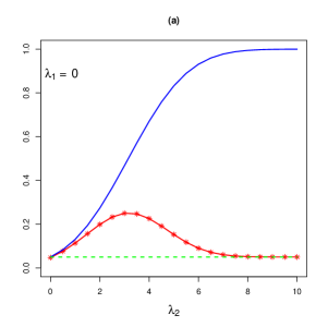
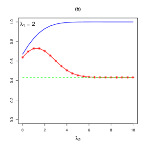
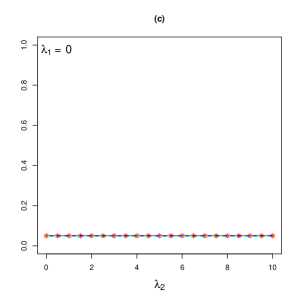
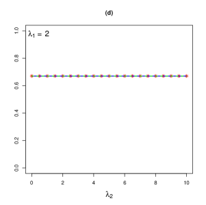
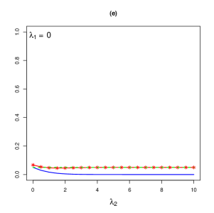
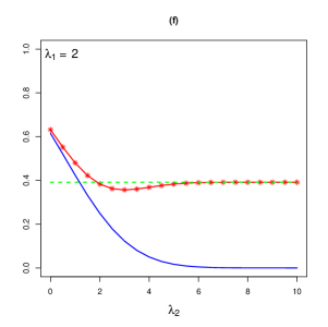
Figure 1: Graphs of power functions as a function of $\lambda_{2}$ for selected values of $\lambda_{1}$ and $\alpha_{1}=\alpha_{2}=\alpha_{3}=\alpha=0.05$. Dotted line, solid line and line with star represent $\Pi^{UT}(\lambda_{1},\lambda_{2})$, $\Pi^{RT}(\lambda_{1},\lambda_{2})$ and $\Pi^{PTT}(\lambda_{1},\lambda_{2})$ respectively. Graphs (a) and (b) are for $\bar{c}>0$, (c) and (d) are for $\bar{c}=0$ and (e) and (f) are for $\bar{c}<0$.

In Figure 1, the power functions for the UT, RT and PTT are plotted against $\lambda_{2}$ at two values of $\lambda_{1}.$ Here $\lambda_{1}=0$ is chosen to study the asymptotic sizes of the tests and we desire the size of a particular test to be small so that the probability of type I error is small. Since we also wish to get small value of probability of type II error, the power of the test at $\lambda_{1}=2$ is considered. An acceptable power function of the test is the one that is small when the null hypothesis is true but large when $\lambda_{1}$ differs much from $\theta=0.$ The first set of regressors is used to plot Figures 1(a) and 1(b). As $\lambda_{2}$ grows larger, $\Pi^{RT}(0,\lambda_{2})$ approaches 1. However, $\Pi^{PTT}(0,\lambda_{2})$, after an initial increase, drops and converges to the nominal size $\alpha=0.05$ as $\lambda_{2}$ grows larger. Thus, the asymptotic size (with very small $\lambda_{1}$) of $\phi_{n}^{PTT}$ is close to $\alpha$ for small $\lambda_{2}$ and large $\lambda_{2}$, while for moderate values of $\lambda_{2}$ it is somehow larger than $\alpha$ but lesser than that of $\Pi^{RT}(0,\lambda_{2})$. The $\Pi^{UT}(0,\lambda_{2})$ is constant and does not depend on $\lambda_{2}.$ The same pattern occurs in Figure 1(b) but the power functions are always significantly larger than $\alpha$, in this case larger than 0.4. If one only considers the size of the test, the PTT is preferred to RT, though the UT remains as the best choice. However, the RT is the best choice but the PTT is preferred to UT if the power of the test at $\lambda_{1}=2$ is considered. It is impossible to obtain a test that uniformly minimizes the size and maximizes the power at the same time. We are looking for a test that is a compromise between minimizing the size and maximizing the power (small probabilities of type I and type II errors). The RT is the best choice for its largest power but the worst choice for its largest size as $\lambda_{2}$ grows larger. On the contrary, the UT is the best choice for its smallest size but the worst choice for its smallest power. Both RT and UT uniformly minimize or maximize the size and power at the same time. The PTT has larger power than the UT for small and moderate values of $\lambda_{2}$ and it has significantly smaller size than that of the RT for moderate and large $\lambda_{2}$. Therefore, if our objective is to obtain a test that has better probabilities for both type I and type II errors, the PTT is suggested as the best option. The PTT is a compromise between minimizing the size and maximizing the power than the RT and UT.

The cases for $\bar{c}=0$ and $\bar{c}<0$ are also considered in this paper, though $\bar{c}>0$ is more important than the other two because it is more realistic. Setting $\bar{c}=0$ in Figures 1(c) and 1(d) imply all power functions remain the same regardless of the value of $\lambda_{2}$ and these constant power functions increase as $\lambda_{1}$ increases. Figures 1(e) and 1(f) illustrate the case when $\bar{c}<0.$ The graphs show that $\Pi^{RT}<\Pi^{PTT}$ for any $\lambda_{2}$ and $\Pi^{PTT}\leq\Pi^{UT}$ for any $\lambda_{2}$ more than a small positive value, say $\lambda_{0}$. The probability of type I error for all test functions are fairly small. The size and power of the RT is decreasing to 0 as $\lambda_{2}$ growing larger (Figures 1(e) and 1(f)) suggesting the RT as the best choice for size but the worst choice for power. Since $\Pi^{PTT}(2,\lambda_{2})\geq\Pi^{RT}(2,\lambda_{2})$ for all $\lambda_{2},$ the PTT is preferred over the RT . Also, $\Pi^{PTT}(2,\lambda_{2})\geq\Pi^{UT}(2,\lambda_{2})$ except for some moderate values of $\lambda_{2}$ but the difference is relatively small. From the examination of all the graphs in Figure 1, the PTT is suggested as the best choice when both probabilities of type I and type II errors are considered.

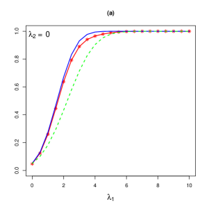
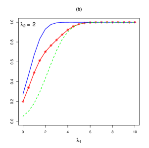
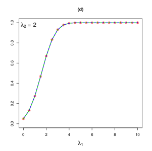
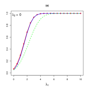
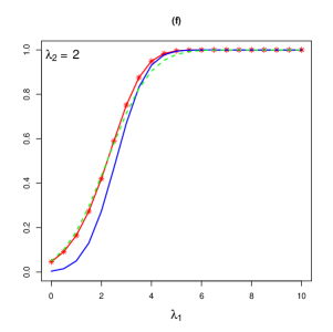
Figure 2: Graphs of power functions as a function of $\lambda_{1}$ for selected values of $\lambda_{2}$ and $\alpha_{1}=\alpha_{2}=\alpha_{3}=\alpha=0.05$. Dotted line, solid line and line with stars represent $\Pi^{UT}(\lambda_{1},\lambda_{2})$, $\Pi^{RT}(\lambda_{1},\lambda_{2})$ and $\Pi^{PTT}(\lambda_{1},\lambda_{2})$ respectively. Graphs (a) and (b) are for $\bar{c}>0$, (c) and (d) are for $\bar{c}=0$ and (e) and (f) are for $\bar{c}<0$.

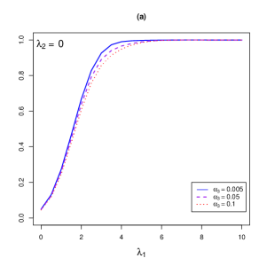
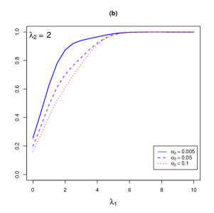
Figure 3: Graphs of power function $\Pi^{PTT}(\lambda_{1},\lambda_{2})$ for nominal sizes $\alpha_{3}=0.005$, 0.05 and 0.1. The $\bar{c}>0$ and $\alpha_{2}=\alpha_{1}=\alpha=0.05$ for all graphs.

The relation between power functions and $\lambda_{1}$ is shown in Fig 2. All power functions are approaching 1 as $\lambda_{1}$ grows larger regardless of the value of $\lambda_{2}.$ This is because the probability of rejecting $H_{0}^{\star}:\theta=0$ increases as $\lambda_{1}$ increases. When $\bar{c}>0$, the probability of type II error for the RT is the smallest, but the PTT is preferable than the UT for all values of $\lambda_{1}$. When $\bar{c}<0$, the PTT is preferable for its comparatively smaller probability of type II error than the other two tests. When $\bar{c}=0,$ all tests have the same probability of type II error regardless of the value of $\lambda_{1}$ (refer to the equation (6.2) for analytical result).

Figure 3 illustrates the behavior of the power function $\Pi^{PTT}(\lambda_{1},\lambda_{2})$ at three different values of nominal size $\alpha_{3}$. The graphs show that the test with smaller nominal significance level has greater power than that of larger significance level. The smaller nominal significance level however increases the probability of type I error as $\lambda_{2}$ moves away from zero. This is illustrated in Fig 3(b), $\Pi^{PTT}(\lambda_{1},2)$ at $\alpha_{3}=0.005,\;\;0.05,\;\mbox{and},\;\;0.1$ start at different values before growing larger and converging to 1.

It is of advantage to study the relationship between the size of the PTT, that is, $\alpha^{PTT}=\Pi^{PTT}(0,\lambda_{2})$ and the nominal significance level of the PT, $\alpha_{3}.$ One may want to know what suppose to be the actual level of significance of the PT that will reject the ultimate test with a predetermined probability, says 5 percent. Taking $\alpha_{1}$ and $\alpha_{2}$ to be equal, here 0.05, the size of the test depends on $\lambda_{2}.$ Figure 4 shows the graphs of $\Pi^{PTT}(0,\lambda_{2})$ against $\alpha_{3}$ for different values of $\lambda_{2}$ with $\alpha_{1}=\alpha_{2}=0.05$ and $\bar{c}>0.$ For smaller values of $\lambda_{2}$, as $\alpha_{3}$ increases, the size of the PTT decreases and reaches its minimum at the value of $\alpha_{3}=\alpha_{3}^{\prime}$ (say), before growing larger and converging to $\alpha=0.05.$ Let the value of $\alpha_{3}$ be $\alpha_{3}^{\prime\prime}$ when the size of the PTT is 0.05, the value of $\alpha_{3}^{\prime\prime}$ increases as $\lambda_{2}$ increases. As we consider larger values of $\lambda_{2}$, the size of the PTT decreases dramatically then slowly converges (appears as flat in the graph) to $\alpha$ at some positive value $\alpha_{3}^{\prime\prime\prime}$. Table 1 gives the values of the size of the PTT at $\alpha_{3}$ for different values of $\lambda_{2},$ with $\alpha_{1}=\alpha_{2}=0.05$ when $\bar{c}>0.$ If we want to reject the ultimate test with significance level 0.05, the nominal significance level of the PT must be set to 0 when $\lambda_{2}$ is 0. Then a larger but still acceptable nominal size $\alpha_{3}$ is required to achieve 5% significance level of the PTT as $\lambda_{2}$ is a bit larger than 0. But up to some point, we cannot sacrifice the increases in the probability of type I error of the PT as $\lambda_{2}$ grows much than 0. As $\lambda_{2}$ grows larger, a larger $\alpha_{3}$ is required to obtain 5% significance level of the PTT (see Table 1). Note: Setting the nominal size of the PT to 0 is meaningless because this means there is no chance that $H_{0}^{(1)}:\beta=0$ is rejected. The size and power of the PTT converges to the RT when $\alpha_{3}$ approaches 0 (refer equation (6.4)), thus supports this result in Table 1.

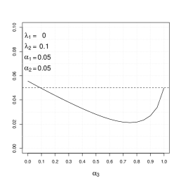
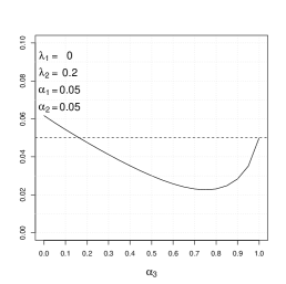
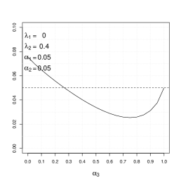
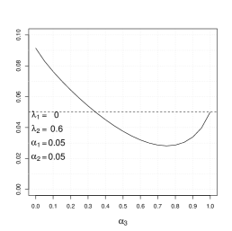
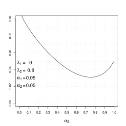
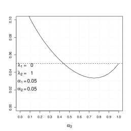
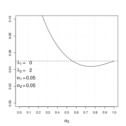
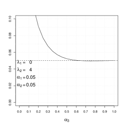
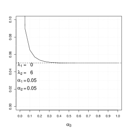
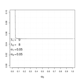
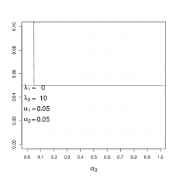
Figure 4: Graphs of size of the PTT $(\alpha^{PTT}=\Pi^{PTT}(0,\lambda_{2}))$ as $\alpha_{3}$ and $\lambda_{2}$ increasing when $\bar{c}>0$ and $\alpha_{1}=\alpha_{2}=0.05$ for all graphs.

Table 1: Size of ultimate test $(\alpha^{PTT})$ as a function of nominal size of PT $(\alpha_{3})$ at selected values of $\lambda_{2}$ and $\alpha_{1}=\alpha_{2}=\alpha=0.05$.

$\lambda_{2}$	$\alpha_{3}$	$\alpha^{PTT}$	$\alpha_{3}$	$\alpha^{PTT}$
0	0.05	0.0479	0.00	0.0500
0.1	0.10	0.0495	0.05	0.0525
0.2	0.20	0.0476	0.15	0.0509
0.4	0.30	0.0475	0.25	0.0515
0.6	0.35	0.0493	0.30	0.0540
0.8	0.40	0.0498	0.35	0.0547
1.0	0.45	0.0491	0.40	0.0543
2.0	0.60	0.0476	0.55	0.0508
4.0	0.65	0.0500	0.60	0.5040
6.0	0.70	0.0500	0.65	0.0500
8.0	0.75	0.0500
10.0	0.75	0.0500

The $\alpha^{PTT}$ is the actual achievable significance level and $\alpha_{3}$ is the nominal PT significance level.

Figure 5 shows graphs of $\alpha^{PTT}=\Pi^{PTT}(0,\lambda_{2})$ for $0\leq\alpha_{3}\leq 1$ at selected values of $\lambda_{2}$, $\alpha_{1}$ and $\alpha_{2}$ when $\bar{c}>0.$ Equations (6.4) and (6.5) show that the size and power of the PTT is approaching the size and power of the RT as the nominal size of PT is closer to 0 but is approaching the size and power of the UT as the nominal size of the PT is closer to 1. From equation (6.4), setting the nominal significance level $\alpha_{3}=0$ implies the size and power of the PTT is entirely contributed by the size and power of the RT and none from the UT. The contribution of the size and power of the UT to the size and power of the PTT is not substantial when the nominal size of the PT is small. From the graphs, the decreasing in the contribution of the size of the RT reduces the size of the PTT as $\alpha_{3}$ differs from zero. On the contrary, setting the nominal size $\alpha_{3}=1$ causes the size of the PTT is totally contributed by the size of the UT (see equation (6.5)). The contribution of the size of the RT is not significant when the nominal size of the PT is large. As the value of $\alpha_{3}$ differs from 1, lesser contribution from the size of the UT imposes smaller size of the PTT. The size of the PTT decreases from both ends and the minimum of the size of the PTT is achieved at a particular value of $\alpha_{3}.$

Further, analysis is carried out to investigate the dependence of the size of the ultimate test to the changes in the nominal sizes $\alpha_{1}$, $\alpha_{2}$ and $\alpha_{3}.$ From observation of Figures 5(a)-5(f), there is an increase in the percentage of $\alpha^{PTT}$ in [0,0.1] for $\alpha_{3}$ in [0,0.2] when we set smaller nominal size of $\alpha_{2}$ for a bit larger value of $\lambda_{2}$. For example, there is 47.62% of $\Pi^{PTT}(0,1)$ in [0,0.10] for $\alpha_{3}$ in [0,0.2] at nominal size $\alpha_{2}=0.05$ (see Figure 5(a)) but there is 100% of $\Pi^{PTT}(0,1)$ when $\alpha_{2}=0.03$ (see Figure 5(b)). For some moderate values of $\lambda_{2}$, there is an increment in the percentage of $\Pi^{PTT}(0,\lambda_{2})$ when we choose a smaller nominal size $\alpha_{2}.$ But only small increment is observed for a larger value of $\lambda_{2}$. For example, there is no $\Pi^{PTT}(0,3)$ in [0,0.10] for $\alpha_{3}$ in [0,0.2] when we set the nominal size to be $\alpha_{2}=0.05$ (see Figure 5(a)) but there is a slightly 4.76% of $\Pi^{PTT}(0,3)$ when $\alpha_{2}=0.03$ (see Figure 5(b)). The small increment suggests setting a much smaller value of nominal size $\alpha_{2}$ maybe necessary to achieve a small size of PTT with small nominal size of pre-test for moderate values of the slope. However, this rule fails for a large value of $\lambda_{2}.$

Table 2: Size of ultimate test $(\alpha^{PTT})$ as a function of nominal size of pre-test $(\alpha_{3})$ at selected values of $\alpha_{2}$ and $\lambda_{2}$ with $\alpha_{1}=0.05$.

$\lambda_{2}=0.5$			$\lambda_{2}=1$			$\lambda_{2}=3$			$\lambda_{2}=6$
$\alpha_{2}$	$\alpha_{3}$	$\alpha^{PTT}$	$\alpha_{2}$	$\alpha_{3}$	$\alpha^{PTT}$	$\alpha_{2}$	$\alpha_{3}$	$\alpha^{PTT}$	$\alpha_{2}$	$\alpha_{3}$	$\alpha^{PTT}$
0.03	0.03	0.0498	0.01	0.00	0.0355	0.01	0.08	0.0994	0.03	0.04	0.0983
	0.02	0.0507		0.01	0.0343		0.07	0.1052		0.03	0.1145
0.04	0.19	0.0499	0.02	0.00	0.0623	0.02	0.15	0.0987	0.04	0.05	0.0891
	0.18	0.0508		0.01	0.0605		0.14	0.1029		0.04	0.1002
0.05	0.31	0.0497	0.03	0.00	0.0870	0.03	0.20	0.0965	0.05	0.05	0.0901
	0.30	0.0507		0.01	0.0839		0.19	0.1005		0.04	0.1014
0.06	0.34	0.0508	0.04	0.02	0.1026	0.04	0.22	0.1007	0.06	0.04	0.1024
	0.04	0.0499		0.03	0.0999		0.23	0.0972		0.05	0.0909
0.07	0.48	0.0491	0.05	0.11	0.0993	0.05	0.25	0.0987	0.10	0.05	0.0093
	0.47	0.0500		0.10	0.1015		0.24	0.1021		0.04	0.1045

The $\alpha^{PTT}$ is the actual achievable significance level and $\alpha_{3}$ is the nominal pre-test significance level.

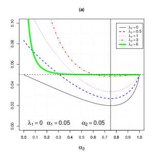
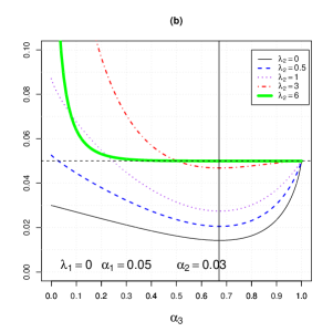
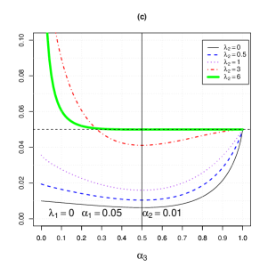
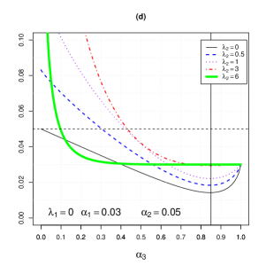
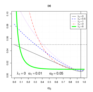
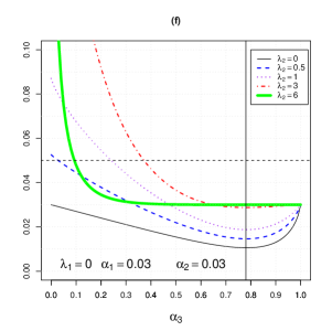
Figure 5: Graphs of the size of ultimate test for increasing $\alpha_{3}$ selected at different values of nominal sizes of $\alpha_{1}$ and $\alpha_{2}$ with $\bar{c}>0$. The intersection with the vertical line represents the minimum.

We wish to have small size of the PTT by setting small nominal sizes of $\alpha_{1},\alpha_{2}$ and $\alpha_{3}.$ Figure 5 shows that this could not be achieved when $\lambda_{2}$ is large and $\alpha_{3}$ is very small (close to zero) even if we set a very small value of $\alpha_{2}$. For instance, there is less than 100% (i.e. 80.95%) of $\Pi^{PTT}(0,6)$ in [0,0.10] as $\alpha_{3}$ in [0,0.2] (see Figures 5(a) and 5(b)) for both nominal sizes $\alpha_{2}=0.03$ and $\alpha_{2}=0.05$. The percentage does not reach 100% even $0<\alpha_{2}<0.03$ is chosen.

Since $\alpha^{PTT}$ behaves like $\alpha^{RT}$ when the nominal size $\alpha_{3}$ is small, the null hypothesis $H_{0}^{\star}:\theta=0$ is rejected more often for small nominal size of $\alpha_{3}$ when $\lambda_{2}$ is large because the nominal size $\alpha_{2}$ is smaller than the actual size of the RT. The null hypothesis $H_{0}^{\star}:\theta=0$ should not be rejected if the true value of $\theta=0.$ In this case, however the possibility of rejection is large when $\lambda_{2}$ differs much from 0 because $\beta=0$ is assumed in the test statistic $T_{n}^{RT}.$ This fact answers the reason why very small $\alpha_{3}$ (close to zero) has a very large size of the test when $\lambda_{2}$ is large.

Table 2 shows the size of ultimate test as a function of nominal size $\alpha_{3}$ for selected values of $\lambda_{2}$ and $\alpha_{2}$ with $\alpha_{1}=0.05$ and $\bar{c}>0$. The nominal sizes for the RT and PT are given in the table for the size of ultimate test near point 0.05 when $\lambda_{2}=0.5$ and 1 and near point 0.10 when $\lambda_{2}=3$ and 6. The table enables us to observe the changes in the values of the nominal size of PT ($\alpha_{3}$) as the nominal size $\alpha_{2}$ changes and the significance level of the PTT is around the same value. We wish to have small nominal size of the PT that allow us to get 5 or 10% of significance level of the PTT. From the table, this is achieved by selecting smaller nominal size of the RT for moderate and small values of slope. When $\lambda_{2}=3$ (moderate value), selecting nominal size $\alpha_{2}$ as small as 0.01 we have as much as 8% of nominal size of the PT to get below than 10% significance level of ultimate test (see Table 2, row:1, col:7-9). In column 1-3 of the table, for $\lambda_{2}=0.5$ (small), approximately 5% level of significance of ultimate test is obtained by setting nominal size of the RT = 0.05 and nominal size of the PT = 0.3 or by setting both nominal sizes of the RT and PT = 0.03 but the latter with smaller nominal sizes of the PT and RT is more preferable. For larger value of the slope, as the nominal size of the PT closer to 0, the size of the PTT is growing too large. When $\lambda_{2}=6$ (large), to obtain at most 10% of significance level of ultimate test, the least nominal size for the PT that we should set is 5% (see Table 2, row:3, col:10-12) when the nominal size $\alpha_{2}$ is set from 0.05 to 0.10.

8 Concluding Remarks

The M-test of the UT, RT and PTT for testing the intercept are provided in this paper. The asymptotic power functions of the tests are derived by using the results from the asymptotic sampling distribution of the statistics.

In the estimation regime, it is well known that the RE has the smallest MSE if distance parameter (a function of $\beta-\beta_{0}$) is 0 or close to 0, but its MSE is unbounded for larger values of the distance parameter. The UE has a constant MSE that does not depend on the distance parameter. The PTE has smaller MSE than that of the RE for moderate and larger values of the distance parameter. The PTE has smaller MSE than the UE if the value of distance parameter is close or equal to 0. In the testing context, the power functions of the UT, RT and PTT demonstrate a similar behavior as the MSE of the UE, RE and PTE.

For a set of realistic values of the regressor, with mean value larger than 0, the size of the RT is small when $\beta=0$ or close to 0, but the size grows large and converges to 1 for larger values of the slope. The UT has a constant size regardless of the value of the slope (via $\lambda_{2}$). The PTT has smaller size than that of the RT when the slope is 0 and very close to 0, and significantly smaller than that of the the RT for moderate and large values of the slope. The PTT has smaller size than the UT for the value of slope is 0 or very close to 0.

Again for a set of realistic values of the regressor, with mean larger than 0, the RT is the best choice for having largest power but the worst choice for having largest size. The size of the UT is constant regardless of the value of the slope. The UT is the best choice for having smallest size but the worst choice for having smallest power. The PTT has smaller size than the RT for moderate and larger values of the slope and has larger power than the UT for smaller and moderate values of the slope. Therefore, the power function of the PTT is found to behave similar to the MSE of the PTE in the sense that though it is not uniformly the best statistical test with the smallest size and the largest power but it protects from the risk of a too large size and a too small power. Thus, the power function of the PTT is a compromise between that of the UT and RT. In the face of uncertainty on the value of the slope, if the objective of a researcher is to minimize the size and maximize the power of the test, the PTT is the best choice.

The tables and graphs support the analytical asymptotic comparison of the UT, RT and PTT as discussed in Section 6. The analysis is furthered by investigating the relationship between the power functions and its arguments, namely the slope and the nominal sizes, of the UT, RT and PT. The chosen values of the nominal sizes that are set before testing affect the actual size of the PTT.

In order to get small probability of type I error for the ultimate test, our investigations concentrate on small nominal sizes of the UT, RT and PT with a view to achieving small (actual) significance level of the PTT. The study revealed that for small and moderate values of slope, the smaller the nominal size of the RT, the smaller the size of the PTT when other nominal sizes are kept fixed and small. For moderate and large values of the slope, a large size of the PTT is observed when nominal size of PT is set close to 0. The size of the PTT behaves much like that of the RT when the nominal size of PT is small, but it behaves more like that of the UT when the nominal size of the PT is large.

The power of the ultimate test is larger for moderate values of the slope than for smaller and larger values of the slope. It is shown analytically that the power of the PTT approaches the power of the RT when the nominal size of PT is closer to 0 but approaches the power of the UT when the nominal size of the PT is closer to 1. In practical applications, size of the PT should be small (ideally close to 0), and in such cases the power of the PTT is close to that of the RT (which is much higher than that of the UT). To avoid the larger size of the RT, practitioners are recommended to use the PTT as it achieves smaller size (than the RT) and higher power (than the UT) when the value of the slope is small or moderate. Even for large values of the slope the PTT has at least as much power as the UT.

Acknowledgements
The authors thankfully acknowledge valuable suggestions of Professor A K Md E Saleh, Carleton University, Canada that helped improve the content and quality of the results in the paper.

References

Bechhofer, R.E. (1951). The effect of preliminary test of significance on the size and power of certain tests of univariate linear hypotheses. Ph.D. Thesis (unpublished), Columbia Univ.

Bozivich, H., Bancroft, T.A. and Hartley, H. (1956). Power of analysis of variance test procedures for certain incompletely specified models. Ann. Math. Statist. 27, 1017 - 1043.

Caroll, R.J. and Rupert, D. (1988). Transformation and Weighting in Regression. Chapman & Hall, US.

H$\acute{a}$jek, J., $\check{S}$id$\acute{a}$k, Z., and Sen, P.K. (1999). Theory of Rank Tests. Academia Press, New York.

Hoaglin, D.C., Mosteller, F. and Tukey, J.W. (1983). Understanding Robust and Explanatory Data Analysis. John Wiley and Sons, US.

Huber, P.J. (1981). Robust Statistics. Wiley, New York.

Jur$\check{e}$ckov$\acute{a}$, J. (1977). Asymptotic relations of M-estimates and R-estimates in linear regression model. Ann. Statist. 5, 464-72.

Jur$\check{e}$ckov$\acute{a}$, J. and Sen, P.K. (1981). Sequential procedures based on M-estimators with discontinuous score functions. J. Statist. Plan. Infer. 5, 253-66.

Jur$\check{e}$ckov$\acute{a}$, J. and Sen, P.K. (1996). Robust Statistical Procedures Asymptotics and Interrelations. John Wiley & Sons, US.

Khan, S., and Saleh, A.K.Md.E. (2001). On the comparison of pre-test and shrinkage estimators for the univariate normal mean. Stat. papers. 42, 451-473.

Khan, S., Hoque, Z., and Saleh, A.K.Md.E. (2002). Estimation of the slope parameter for linear regression model with uncertain prior information. J. Stat. Res. 36, 55-74.

Saleh, A.K.Md.E. and Sen, P.K. (1982). Non-parametric tests for location after a preliminary test on regression. Communications in Statistics: Theory and Methods. 11, 639-651.

Saleh, A.K.Md.E. (2006). Theory of Preliminary test and Stein-type estimation with applications. John Wiley & Sons, New Jersey.

Schrader, R. M. and Hettmansperger, T.P. (1980). Robust analysis of variance based upon a likelihood ratio criterion. Biometrika. 67, 93-101. sen82 Sen. P.K. (1982). On M-tests in linear models. Biometrika. 69, 245-248.

Sen, P.K. and Saleh, A.K.Md.E. (1987). On preliminary test and schrinkage M-estimation in linear models. Ann. Statist. 15, 1580-1592.

van der Vaart, A.W. (1998). Asymptotic statistics. Cambridge University Press, UK. wilcox05 Wilcox, R.R. (2005). Introduction to Robust Estimation and Hypothesis Testing. Elsevier Inc, US.