Evaluate the Word Error Rate of Binary Block Codes with Square Radius Probability Density Function

Abstract

The word error rate (WER) of soft-decision-decoded binary block codes rarely has closed-form. Bounding techniques are widely used to evaluate the performance of maximum-likelihood decoding algorithm. But the existing bounds are not tight enough especially for low signal-to-noise ratios and become looser when a suboptimum decoding algorithm is used. This paper proposes a new concept named square radius probability density function (SR-PDF) of decision region to evaluate the WER. Based on the SR-PDF, The WER of binary block codes can be calculated precisely for ML and suboptimum decoders. Furthermore, for a long binary block code, SR-PDF can be approximated by Gamma distribution with only two parameters that can be measured easily. Using this property, two closed-form approximative expressions are proposed which are very close to the simulation results of the WER of interesting.

I Introduction

The performance evaluation of binary block codes with soft-decision-decoding in additive white Gaussian noise (AWGN) and fading channels has long been a problem in coding theory and practice. A closed-form expression of word error rate (WER) for popularly used long codes hasn’t been derived as yet. Thus, bounding techniques are widely used for performance evaluation of maximum-likelihood (ML) decoding. The most popular upper bound is the union bound. When the weight enumerating function of a code is known, union bound presents a tight upper bound at signal-to-noise ratios (SNRs) above the cutoff rate limit but becomes useless at SNRs below the cutoff rate limit [1]. Based on Gallager’s first bounding technique [2], some tighter upper bounds are presented [3][4][5]. These bounds are tighter relative to union bound. But even Poltyrev’s tangential sphere bound [6], which has been believed as the tightest bound for binary block codes, still has a gap to the real value of WER [7][8][9]. Additionally, these bounds are all based on ML decoding, which is too complex to implement in practice. When a suboptimum decoder is used, the WER will change but these bounds still keep their original value.

In this paper, a new concept named square radius probability density function (SR-PDF) of decision region is proposed to calculate the WER precisely at SNRs of interesting and any decoding algorithm. The basic premise is that in AWGN channel, when the encoder and decoding algorithm are given, the decision region is fixed, and WER is completely determined by the decision region. The SR-PDF proposed in this paper is unique for every encoder-channel-decoder models, thus any changes of channel and decoding algorithm can be reflected by it. Furthermore, when the codeword length $N\rightarrow\infty$, the asymptotic WER is exactly the complementary cumulative distribution probability of the normalized square radius and can be roughly characterized by the maximum point of the SR-PDF. Moreover, for popular long codes such as Turbo codes, Low-density parity check (LDPC) codes and Convolutional codes, etc, their SR-PDFs are close to Gamma distribution, which implies that the exhausting measurement of SR-PDF is not needed, and only the mean and variance of the square radius are enough to get an approximated SR-PDF. Based on these properties, two closed-form approximative expressions of WER are proposed and their approximation errors are around the order of 0.1dB and 0.3dB respectively for WER above $10^{-3}$.

The rest of this paper is organized as follows: Section II introduces the system model and the concept of SR-PDF of decision region, as well as the method of measuring the pdf. In section III, the WER in AWGN channel is derived using SR-PDF and several examples are followed to prove the validity of the proposed method. Section IV illustrates some important asymptotic properties of the relation of WER to the normalized SR-PDF. In section V, two closed-form approximative expressions are derived for WER calculation. Section VI extending the SR-PDF method to flat fading channel. The conclusion is drawn in section VII, including some discussion and remarks on the SR-PDF method and other applications.

II Preliminaries

II-A System Model

The following system model is used in the paper. Binary information bits are first encoded to binary block code. The code rate is $R=k/N$, where $N$ is the codeword length and $k$ is the information length. Then encoded bits are BPSK modulated (the resulting signal set is ${\rm{\bf S}}$), and transmitted in AWGN channel. The received signal is

$${\rm{\bf y}}={\rm{\bf s}}+{\rm{\bf n}}$$ (1)

where ${\rm{\bf s}}=\left[{s_{1},s_{2},...,s_{N}}\right]^{T}\in{\rm{\bf S}}$, $s_{i}\in\{\pm\sqrt{E_{s}}=\pm\sqrt{RE_{b}}\}$, $E_{s}$ and $E_{b}$ are, respectively, the energy per code bit and the energy per information bit. ${\rm{\bf n}}=\left[{n_{1},n_{2},...n_{N}}\right]^{T}$ is the additive white Gaussian noise with zero-mean and variance $\frac{N_{0}}{2}$. In this paper, SNR (signal to noise power ratio) is defined as $\beta=\frac{2E_{s}}{N_{0}}$. It is also assumed that the signal $\bf s$ is detected coherently and decoded with some algorithm at the receiver, and the channel side information is known if it is required.

II-B Decision Region and Square Radius Probability Density Function

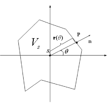
The decision region $V_{s}$ of signal ${\rm{\bf s}}$ is a set in $N$ dimensional Euclidean space ${\bf R}^{N}$. Consider the decoder as a function that maps the received vector $\rm{\bf y}$ to a transmitted signal $\rm{\bf s}\in\rm{\bf S}$, $f_{decoder}:{\bf R}^{N}\rightarrow\bf S$, then the decision region can be defined as $V_{s}=\left\{{\bf y}|{\bf y}\in{\bf R}^{N},f_{decoder}(\rm{\bf y})={\rm{\bf s}}\right\}$, i.e. the domain of $\bf s$. Whenever the decoder is specified, the decision region is fixed. When the received vector ${\rm{\bf y}}$ lies inside $V_{s}$, it will be correctly decoded to ${\rm{\bf s}}$, otherwise a decoding error occurs. For linear block codes investigated in this paper, all the codewords have the same decision region. Fig. 1 is an example of two dimensional decision region, where ${\rm{\bf n}}$ is the additive noise, ${\rm{\bf\theta}}$ is the direction of ${\rm{\bf n}}$. Point ${\rm{\bf p}}$ is on the boundary of decision region and the radial originated from ${\rm{\bf s}}$ along ${\rm{\bf\theta}}$. Connecting ${\rm{\bf s}}$ and ${\rm{\bf p}}$, the length of vector ${\rm{\bf r}}({\rm{\bf\theta}})$ is the radius of the decision region along the direction of ${\rm{\bf n}}$. Define $l({\rm{\bf\theta}})=\left|{{\rm{\bf r}}({\rm{\bf\theta}})}\right|^{2}$ as the square radius in the direction of $\theta$. Because $\bf n$ is a random variable, so $l(\theta)$ is a random variable. The pdf of $l({\rm{\bf\theta}})$ is denoted as $p_{l}(l)$ and is abbreviated as SR-PDF. This concept can be extended to $N$ dimensional space, where $\uptheta$ is determined by $N-1$ angles (e.g. azimuth and elevation in three dimensional space).

The SR-PDF is too complex to work out in analytical way for long codes, but it can be measured with simulation: For the system model above, generate a white Gaussian noise vector ${\rm{\bf n}}=(n_{1},n_{2},...n_{N})$, normalize $\bf{n}$ to ${\rm{\bf{n}^{\prime}}}=\frac{{\rm{\bf n}}}{\left|{\rm{\bf n}}\right|}=(1,{\rm{\bf\uptheta}})$, where ${\rm{\bf\uptheta}}$ is the direction of ${\rm{\bf n}}$, scale ${\rm{\bf{n}^{\prime}}}$ by $\lambda$ and send the vector ${\rm{\bf y}}={\rm{\bf s}}+\lambda{\rm{\bf{n}^{\prime}}}$ to the decoder. There exists a $\hat{\lambda}>0$ such that $f_{decoder}({\bf s}+\lambda{\bf n}^{\prime})={\bf s},~{}\forall\lambda\leq\hat{\lambda}$ and $f_{decoder}(\bf{s}+\lambda\bf{n}^{\prime})\neq{\bf s},~{}\forall\lambda>\hat{\lambda}~{}$. In this paper, we will assume that the decision region is simply connected. Consequently, $|{\rm{\bf r}}({\rm{\bf\uptheta}})|=\hat{\lambda}$ is the radius in direction of $\bf n$, and $l(\uptheta)=\hat{\lambda}^{2}$ is the square radius. Note that $\bf r(\uptheta)$ is related to the code bit energy and codeword length. This effect can be removed by normalizing the square radius by $NE_{s}$, i.e. $l_{n}=\frac{l}{NE_{s}}$. The resulting SR-PDF is referred to as normalized SR-PDF and is denoted as $p_{l_{n}}(l_{n})$ hereafter. With sufficient tests, the approximated normalized SR-PDF can be obtained.

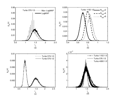
Fig. 2 is the normalized SR-PDF of Turbo codes with different codeword lengths, code rates and decoding algorithms in AWGN channel. Turbo codes used in this paper is defined in [13]. Obviously, all the changes in the encoder and decoder will be reflected by the SR-PDF. Larger decision region implies that the code can tolerate larger noise, therefore, the SR-PDF which occurs in the righter side will have a better WER performance. Subsequent sections will mainly discuss the relation between SR-PDF and WER.

III Word Error Rate In AWGN Channel

In AWGN channel, the decision region and the corresponding SR-PDF is completely determined whenever the decoder is specified, no matter whether it is a maximum likelihood (ML) decoder like the Viterbi decoding for Convolutional codes or a suboptimal decoder such as the iterative decoders for Turbo and LDPC codes. For a binary linear block code, all the codewords have the same error rate. Therefore, without loss of generality, assume a codeword $\bf{s}\in\bf{S}$ is transmitted. The word error rate is the probability that the received vector ${\bf y}\notin V_{s}$ conditioned on ${\bf s}$, that is

$$\begin{split}P_{e}&=1-\oint\limits_{V_{s}}{p\left({{\rm{\bf y}}|{\rm{\bf s}}}\right)d{\rm{\bf y}}}\\ &=1-\oint\limits_{V_{s}-s}{p\left({{\rm{\bf y}}-{\rm{\bf s}}}\right)d{\rm{\bf y}}}\\ &=1-\oint\limits_{V_{s}^{{}^{\prime}}}{p\left({\rm{\bf n}}\right)d{\rm{\bf n}}}\\ \end{split}$$ (2)

where $V_{s}^{{}^{\prime}}=V_{s}-s$ is the shift of the decision region from $s$ to origin. Denoting ${\rm{\bf n}}$ in polar coordinates, (2) becomes

$$\begin{split}P_{e}&=1-\oint\limits_{V_{s}^{{}^{\prime}}}{p_{\rho,{\rm{\bf\uptheta}}}\left({\rho,{\rm{\bf\uptheta}}}\right)d\rho d{\rm{\bf\uptheta}}}\\ &=1-\oint\limits_{V_{s}^{{}^{\prime}}}{p_{\rho|{\rm{\bf\uptheta}}}\left(\rho\right)p_{\rm{\bf\uptheta}}({\rm{\bf\uptheta}})d\rho d{\rm{\bf\uptheta}}}\\ &=1-\int_{\rm{\bf\uptheta}}{\left[{\int_{\rho\leq|r({\rm{\bf\uptheta}})|}{p_{\rho|{\rm{\bf\uptheta}}}\left(\rho\right)d\rho}}\right]p_{\rm{\bf\uptheta}}\left({\rm{\bf\uptheta}}\right)d{\rm{\bf\uptheta}}}\\ &=\int_{\rm{\bf\uptheta}}{\left[{\int_{\rho>|r({\rm{\bf\uptheta}})|}{p_{\rho|{\rm{\bf\uptheta}}}\left(\rho\right)d\rho}}\right]p_{\rm{\bf\uptheta}}\left({\rm{\bf\uptheta}}\right)d{\rm{\bf\uptheta}}}\\ &=E_{\rm{\bf\uptheta}}\left[{\int_{\rho>|r({\rm{\bf\uptheta}})|}{p_{\rho|{\rm{\bf\uptheta}}}\left(\rho\right)d\rho}}\right]\\ \end{split}$$ (3)

Note that the integral in the bracket is the decoding error probability conditioned on the direction of a noise realization, so

$$\begin{split}P_{e|{\rm{\bf\uptheta}}}&=\int_{\rho>|r({\rm{\bf\uptheta}})|}{p_{\rho|{\rm{\bf\uptheta}}}\left(\rho\right)d\rho}\\ &=P\left[{\rho\geq\left|{r({\rm{\bf\uptheta}})}\right|}\right]\\ &=P\left[{\rho^{2}\geq l({\rm{\bf\uptheta}})}\right]\\ \end{split}$$ (4)

Expectation over ${\rm{\bf\uptheta}}$ is equivalent to expectation over $l$, thus the average error probability is

$$\begin{split}P_{e}&=E_{\uptheta}\left[{P_{e|{\rm{\bf\uptheta}}}}\right]=E_{l}\left[{P\left({\rho^{2}\geq l}\right)}\right]\\ &=\int_{0}^{\infty}{P\left({\rho^{2}\geq x}\right)p_{l}\left(x\right)dx}\\ &=\int_{0}^{\infty}{P\left({\rho^{2}\geq NE_{s}x}\right)p_{l_{n}}\left(x\right)dx}\\ \end{split}$$ (5)

where $\rho^{2}=\left|{\rm{\bf n}}\right|^{2}=\sum\limits_{i=1}^{N}{n_{i}^{2}}$. Define $x=\rho^{2}$, then $x$ is chi-square distributed [11] with $N$ degrees of freedom. The pdf of $x$ is

$$p(x)=\frac{1}{N_{0}^{N/2}\Gamma\left({N\mathord{\left/{\vphantom{N2}}\right.\kern-1.2pt}2}\right)}x^{N\mathord{\left/{\vphantom{N2}}\right.\kern-1.2pt}2-1}e^{-x\mathord{\left/{\vphantom{x{N_{0}}}}\right.\kern-1.2pt}{N_{0}}},\mbox{ }x\geq 0$$ (6)

where $\Gamma(x)$ is the gamma function [12]. When $x$ is an integer and $x>0$, $\Gamma(x+1)=x!$ (the factorial of $x$). So

$$\begin{split}P_{e|{\rm{\bf\uptheta}}}&=P\left[{\rho^{2}\geq l}\right]\\ &=1-\int_{0}^{NE_{s}l_{n}}{\frac{1}{N_{0}^{N/2}\Gamma\left({N\mathord{\left/{\vphantom{N2}}\right.\kern-1.2pt}2}\right)}x^{N/2-1}e^{-x/N_{0}}}dx\\ &=1-\frac{1}{\Gamma\left({N\mathord{\left/{\vphantom{N2}}\right.\kern-1.2pt}2}\right)}\int_{0}^{N\beta l_{n}/2}{e^{-x}x^{\frac{N}{2}-1}dx}\\ &=1-\frac{1}{\Gamma\left({N\mathord{\left/{\vphantom{N2}}\right.\kern-1.2pt}2}\right)}\gamma\left({\frac{N}{2},\frac{N\beta l_{n}}{2}}\right)\\ \end{split}$$ (7)

where $\gamma(\alpha,x)$ is the incomplete gamma function defined as [12]

$$\gamma(\alpha,x)=\int_{0}^{x}{e^{-t}t^{\alpha-1}dt},\quad\alpha>0$$ (8)

when $\alpha$ is an integer [12],

$$\gamma(\alpha,x)=(\alpha-1)!\left(1-e^{-x}\sum\limits_{m=0}^{\alpha-1}{\frac{x^{m}}{m!}}\right)$$ (9)

substitute (7) into (5),

$$P_{e}=E_{\uptheta}\left[P_{e|\uptheta}\right]=E_{l}\left[P\left(\rho^{2}>l\right)\right]=\int_{0}^{\infty}{\left[{1-\frac{1}{\Gamma\left({N\mathord{\left/{\vphantom{N2}}\right.\kern-1.2pt}2}\right)}\gamma\left({\frac{N}{2},\frac{N\beta x}{2}}\right)}\right]p_{l_{n}}(x)}dx$$ (10)

(10) show that, WER of linear binary codes under AWGN channel is completely determined by the normalized SR-PDF through a one dimensional integral.

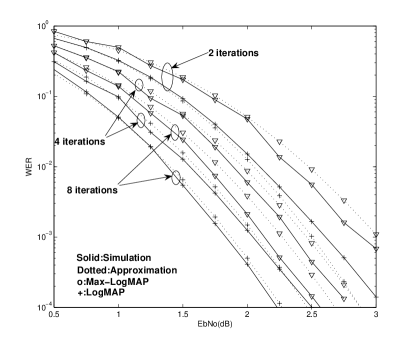
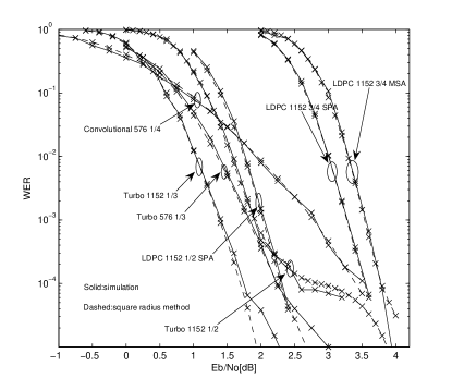
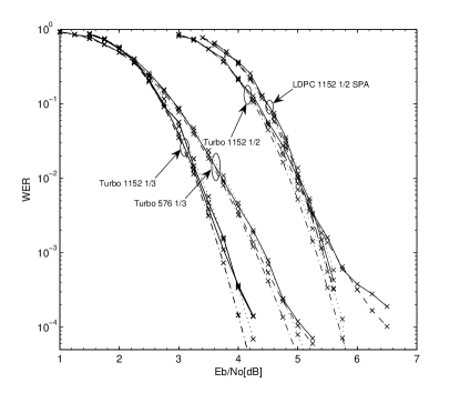
Simulations are used to verify (10). Three error control codes commonly used in wireless communications are considered, including Convolutional codes [12], Turbo codes [12] and LDPC codes [14]. Fig. 3 is the comparison of WER between simulation and that evaluated from (10). For the simulation, each point on the curve is obtained by $10^{6}$ tests; For the results of (10), $10^{5}$ radius are measured to get $p_{l_{n}}(l_{n})$, which is then substituted into (10) to get the WER. Fig. 3 shows the WER of Turbo code for different maximum iterations. The parameter is $N=576$, $R=1/3$ and the decoding algorithms are Log-MAP and Max-log-MAP. Fig. 3 are the WERs of Turbo, LDPC and Convolutional codes with different code lengths and code rates. The decoding algorithms are log-MAP with 8 maximum iterations for turbo code, soft Viterbi algorithm for Convolutional code, sum-product algorithm (SPA) and min-sum algorithm (MSA) with 25 maximum iterations and layered decoding for LDPC codes. It can be seen from these figures that the WER evaluated from (10) matches very well with the simulation results except for large SNRs. The mismatch in large SNR region maybe caused by the inaccurateness of the simulation, or the inaccurateness of the “left tail” (this will be further explained in section IV) of $p_{l_{n}}(l_{n})$, both of which are difficult to be measured precisely owning to infinitesimal probability. Moreover, the SR-PDF method can trace the change of decoder, e.g. the number of iterations, any modifications of the algorithm and etc. while the bounds such as union bound and so on cannot do this.

IV Asymptotic Properties of WER

Eq.(10) shows that the WER of a binary linear code is completely determined by the normalized SR-PDF, $p_{l_{n}}(x)$. When the codeword length, $N\rightarrow\infty$, there are some asymptotic properties of WER which will be discussed in this section.

Property 1

Define $\tau=1/\beta$ and $P_{e}^{a}$ as the WER when codeword length $N\rightarrow\infty$, i.e. $P_{e}^{a}(\tau)=\lim\limits_{N\rightarrow\infty}P_{e}(N,\beta)$ where $P_{e}(N,\beta)$ is defined by (10). Then, $P_{e}^{a}(\tau)$ is exactly the cumulative distribution function (CDF) of the normalized square radius:

$$P_{e}^{a}(\tau)=\lim_{N\rightarrow\infty}P_{e}(N,\beta)=\int_{0}^{1/\beta}p_{l_{n}}(x)dx=\int_{0}^{\tau}p_{l_{n}}(x)dx=F_{l_{n}}(\tau),$$ (11)

where $F_{l_{n}}(x)$ is the CDF of normalized square-radius $l_{n}$.

Proof:

Define

$$f(\alpha,t)\triangleq{\frac{1}{\Gamma(\alpha)}}\gamma(\alpha,\alpha t)=\frac{\int_{0}^{\alpha t}e^{-x}x^{\alpha-1}dx}{\Gamma(\alpha)},\quad t\geq 0,~{}\alpha>0$$ (12)

It is obvious that $f(\alpha,0)=0$ and $f(\alpha,\infty)=1$. Taking derivative with respect to $t$,

$$\frac{\partial f}{\partial t}=\frac{\alpha e^{-\alpha t}(\alpha t)^{\alpha-1}}{\Gamma(\alpha)},\quad t\geq 0$$ (13)

For a large $\alpha$, $\Gamma(\alpha)$ can be approximated with Stirling’s Series [12]

$$\Gamma(\alpha)=e^{-\alpha}\alpha^{\alpha-\frac{1}{2}}\sqrt{2\pi}\left(1+\frac{1}{12\alpha}+\frac{1}{288\alpha^{2}}-\cdots\right)\approx e^{-\alpha}\alpha^{\alpha-\frac{1}{2}}\sqrt{2\pi}$$ (14)

Substitute into (13)

$$\frac{\partial f}{\partial t}=\frac{\alpha e^{-\alpha t}(\alpha t)^{\alpha-1}}{e^{-\alpha}\alpha^{\alpha-\frac{1}{2}}\sqrt{2\pi}}=\sqrt{\frac{\alpha}{2\pi t^{2}}}\left(te^{1-t}\right)^{\alpha},\quad t\geq 0$$ (15)

The term $te^{1-t}$ is always less than 1 when $t\neq 1$. Thus,

$$\mathop{\lim}\limits_{\alpha\to\infty}\frac{\partial f}{\partial t}=\begin{cases}0\quad\ t\neq 1\\ \infty\quad t=1\end{cases}$$ (16)

$f(\alpha,t)$ is a continuous function of $t$. Therefore, as $\alpha$ approaches infinity, $f(\alpha,t)$ approaches to a unit step function:

$$\mathop{\lim}\limits_{\alpha\to\infty}{\frac{1}{\Gamma(\alpha)}}\gamma(\alpha,\alpha t)=\begin{cases}f(\alpha,\infty)=1\quad t>1\\ f(\alpha,0)=0\quad\ 0\leq t<1\end{cases}$$ (17)

Applying (17) to (10) will obtain (11). ∎

This property can also be explained with the law of large numbers: Dividing $\rho^{2}$ and $l\left({\rm{\bf\uptheta}}\right)$ in (7) by codeword length $N$

$$P_{e|{\rm{\bf\uptheta}}}=P\left[{\frac{\rho^{2}}{N}>\frac{l({\rm{\bf\uptheta}})}{N}}\right]$$ (18)

because $\rho^{2}=\sum\limits_{i=1}^{N}{n_{i}^{2}}$, where $n_{i}^{2},i=1,2,...N$ are independent and identically distributed (i.i.d) variables and $E(n_{i}^{2})=\frac{N_{0}}{2}$, based on the law of large numbers

$$\mathop{\lim}\limits_{N\to\infty}P\left\{{\left|{\frac{\sum\limits_{i=1}^{N}{n_{i}^{2}}}{N}-\frac{N_{0}}{2}}\right|=\left|{\frac{\rho^{2}}{N}-\frac{E_{s}}{\beta}}\right|<\varepsilon}\right\}=1$$ (19)

where $\varepsilon$ is a positive number arbitrarily small. (19) implies that $\frac{\rho^{2}}{N}$ approaches a constant, $\frac{E_{s}}{\beta}$, as $N$ approaches infinity. Based on (18) and (19)

$$\begin{split}\mathop{\lim}\limits_{N\to\infty}P_{e|{\rm{\bf\uptheta}}}&=P\left[{\frac{l(\uptheta)}{N}<\frac{E_{s}}{\beta}}\right]=P\left[{l_{n}(\uptheta)<\frac{1}{\beta}}\right]\\ &=\begin{cases}1&\frac{1}{\beta}>l_{n}(\uptheta)\\ 0&\text{else}\end{cases}\end{split}$$ (20)

Substituting (20) into (10) will get (11).

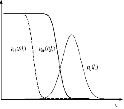
The conditional WER (7), i.e. the term in the square bracket of (10) is a decreasing function around $l_{n}=1/\beta$ with respect to $l_{n}$. This is illustrated in Fig.5 together with the SR-PDF $p_{l_{n}}(l_{n})$. The WER of (10) is the integral of the product $P_{e|\theta}(\beta l_{n})p_{l_{n}}(l_{n})$. It is clear that when SNR is high, WER is dominated by the left tail of the normalized SR-PDF.

Property 2

The inflection point $\tau_{0}$ of $P_{e}^{a}(\tau)$, is the maximum point of the normalized SR-PDF.

Proof:

Based on property 1, taking the second derivative of (11) with respect to $\tau$

$$\frac{\text{d}^{2}P_{e}^{a}(\tau)}{\text{d}\tau^{2}}=\frac{\text{d}p_{l_{n}}(\tau)}{\text{d}\tau}=0$$ (21)

The result $\tau_{0}$ that make (21) equal to zero is the inflection point of $P_{e}^{a}$ and must be the maximum point of $p_{l_{n}}(\tau)$. ∎

The inflection point $\tau_{0}$ tells the position where the WER curve falls rapidly. Define critical SNR as the inverse of the inflection point:

$$\beta_{c}=1/\tau_{0}$$ (22)

then $\beta_{c}$ can be viewed as a single parameter which can be used to characterize the WER performance of long codes. This has been shown in Fig. 6, where we have drawn the simulated WER with liner coordinates. For the popular codes, the normalized SR-PDF tends to be symmetric about the maximum point and the normalized SR-PDF $p_{l_{n}}(x)$ arrives to its maximum roughly at $\mu_{l_{n}}=E[l_{n}]$. Thus, the critical SNR of a code can be approximated as $\beta_{c}\approx\frac{1}{\mu_{l_{n}}}$. The critical SNRs of the codes in Fig. 3 are listed in Table I.

Property 3

For the capacity achievable codes, decision region is a multi-dimensional sphere with constant radius. The inverse of the normalized square radius, i.e. the critical SNR $\beta_{c}$, is the Shannon limits. By ”Shannnon limit”, it means such a threshold SNR $\beta_{s}$ that for a given family of codes with fixed code rate and codeword length $N\rightarrow\infty$, if the channel SNR is greater than $\beta_{s}$, the code will be decoded successfully, otherwise, if SNR is less than $\beta_{s}$, the decoding process will fail.

Proof:

Based on 10 and 35

$$P_{e}^{a}(\tau)=\int_{0}^{1/\beta}p_{l_{n}}(x)dx=\begin{cases}1\quad\beta\leq\beta_{c}\\ 0\quad\beta>\beta_{c}\end{cases}$$ (23)

The $\beta_{s}$ that satisfy 23 is unique for the given family of codes, thus with the definition of $\beta_{s}$, it is clearly that $\beta_{s}=\beta_{c}$. 23 implies that $p_{l_{n}}(x)=\delta(x-\frac{1}{\beta_{s}})$, where $\delta(x)$ is the Dirac impulse function. A random variable with $\delta$ pdf is in fact a constant which is also the mean. Thus the decision region must be a sphere with constant radius. ∎

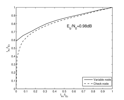
It is well known that threshold SNR of iterative soft-decision decoding can be obtained by means of Density Evolution [16][17] or the equivalent (Extrinsic Information Transfer) EXIT chart [18][19][20]. So property 3 implies that measuring the average square radius of the decision region is another way to determine threshold SNR. For the Turbo code in Table I, which is exactly the same as the one used in [17], the threshold SNR obtained with Density Evolution can be found in [17] as 0.70dB for 1/2 code rate and 0.02dB for 1/3 code rate, the difference with $\beta_{c}$ is within 0.07dB. For the 1/2 code rate LDPC code in Table I, its EXIT chart is shown in Fig.4, where the two curves intersect until $I_{E_{v}}=1$ implying that the threshold SNR is about 0.98dB, while the critical SNR obtained from $\mu_{l_{n}}$ is 0.92dB, the difference is 0.06dB.

Note that though the threshold SNR is generally viewed as a kind of analytical value, this value can only be obtained via numerical simulations with possible approximations (such as Gaussian approximation [16][17]). Therefore, it is hard to say which one among $\beta_{c}$ and $\beta_{s}$ is more accurate.

Property 3 has provided us a simple method to estimate the asymptotic performance (Shannon limit) for a given family of code. We only need to measure the mean of the square-radius with a code of adequate length because the mean is independent of codeword length if the code family is given. Note that measuring the mean is much simpler than measuring the pdf, with our experience, 1000 radius is enough to get a relatively accurate result.

The difference between good codes (the codes that can achieve Shannon limits when $N\rightarrow\infty$) and practical codes is that, The WER of good codes falls steeply at the critical SNR while the WER of practical codes falls in a rolling off fashion around the critical SNR. Define $\Delta_{\epsilon}$ as the range corresponding to $P_{e}^{a}(\tau)$ falls from $1-\epsilon$ to $\epsilon$, where $0<\epsilon\ll 1$, i.e.

$$\Delta_{\epsilon}\triangleq\tau_{1-\epsilon}-\tau_{\epsilon}=F_{l_{n}}^{-1}(1-\epsilon)-F_{l_{n}}^{-1}(\epsilon)$$ (24)

Then $\Delta_{\epsilon}$ can be viewed as a measure of perfectness of practical codes compared with the good codes. If the code is capacity achievable, the WER is a step function thus $\Delta_{\epsilon}=0$. Otherwise, $\Delta_{\epsilon}$ will be a positive number. The $\Delta_{\epsilon}$ for codes in Fig. 3b are listed in table I.

Assume that $p_{l_{n}}(\tau)$ is symmetrical about the mean $\mu_{l_{n}}$ when codeword length $N\rightarrow\infty$, $\Delta_{\epsilon}$ is bounded by

$$\Delta_{\epsilon}\leq\sqrt{2\sigma_{l_{n}}^{2}/\epsilon}$$ (25)

where $\sigma_{l_{n}}^{2}$ is the variance of $l_{n}$. This is because that, with the Chebyshev Inequality:

$$2\epsilon=P\left\{|\tau-\tau_{0}|\geq\frac{\Delta_{\tau}}{2}\right\}\leq\frac{4\sigma_{l_{n}}^{2}}{\Delta_{\tau}^{2}}$$ (26)

In practice, the WER falling range in decibel domain may be more interesting, i.e.

$$\Delta_{\epsilon\text{(dB)}}\triangleq 10\log_{10}\frac{\tau_{2}}{\tau_{1}}=10\log_{10}\frac{F_{l_{n}}^{-1}(1-\epsilon)}{F_{l_{n}}^{-1}(\epsilon)}$$ (27)

The Chebyshev bound now changes to

$$\Delta_{\epsilon\text{(dB)}}\leq 10\text{log}_{10}\left(\frac{\tau_{0}+\frac{\Delta_{\tau}}{2}}{\tau_{0}-\frac{\Delta_{\tau}}{2}}\right)=10\text{log}_{10}\left(\frac{\mu_{l_{n}}+\sigma_{l_{n}}\sqrt{1/2\epsilon}}{\mu_{l_{n}}-\sigma_{l_{n}}\sqrt{1/2\epsilon}}\right)\rm{dB}.$$ (28)

The bounds in dB for codes in Fig. 3b are also listed in table I. It is obvious that the bound is quite loose, roughly $3\thicksim 5$ times larger.

V Approximation of WER

Eq.(10) involves an integration of the product of incomplete gamma function and SR-PDF. Moreover, accurate measurement of SR-PDF requires a large number of decoding tests. Thus, it is inconvenient for practical use, and approximation formulas will be welcome. The approximation of (10) is to approximate the normalized SR-PDF $p_{l_{n}}(x)$. Although other approximations such as Gaussian are also possible, it is found that Gamma approximation is more accurate. The pdf of Gamma distribution is given by

$$p(x)=\frac{1}{b^{a}\Gamma(a)}x^{a-1}e^{-\frac{x}{b}}$$ (29)

where $a$ and $b$ are the parameters of Gamma distribution that have the following relationship with $\mu_{l_{n}}$ and $\sigma_{l_{n}}^{2}$ [15]:

$$\begin{cases}a=\mu_{l_{n}}^{2}/\sigma_{l_{n}}^{2}\\ b=\sigma_{l_{n}}^{2}/\mu_{l_{n}}\end{cases}$$ (30)

Substitute (29) into (10),

$$P_{e}\approx\int_{0}^{\infty}{\frac{1}{b^{a}\Gamma(a)}x^{a-1}e^{-\frac{x}{b}}\left[{1-\frac{1}{\Gamma\left({N\mathord{\left/{\vphantom{N2}}\right.\kern-1.2pt}2}\right)}\gamma\left({\frac{N}{2},\frac{N\beta x}{2}}\right)}\right]dx}$$ (31)

For long codes, increasing code length from $N$ to $N+1$ generally brings no notable performance difference. So assuming that $N$ is even and recalling (9), the WER can be simplified as

$$\begin{split}P_{e}&\approx\sum\limits_{m=0}^{\frac{N}{2}-1}{\frac{\left(\frac{N\beta}{2}\right)^{m}}{b^{a}\Gamma(a)m!}\int_{0}^{\infty}{x^{m+a-1}e^{-x(\frac{1}{b}+\frac{N\beta x}{2})}}}dx\\ &=\sum\limits_{m=0}^{\frac{N}{2}-1}{\frac{\left(\frac{N\beta}{2}\right)^{m}\left({\frac{2b}{2+N\beta b}}\right)^{m+a}\Gamma(m+a)}{b^{a}\Gamma(a)\Gamma(m+1)}\int_{0}^{\infty}\frac{1}{\left({\frac{2b}{2+N\beta b}}\right)^{m+a}\Gamma(m+a)}{x^{m+a-1}e^{-\frac{x(2+N\beta b)}{2b}}}}dx\\ &=\sum\limits_{m=0}^{\frac{N}{2}-1}\frac{\left(1-u\right)^{m}u^{a}}{mB(a,m)}\\ \end{split}$$ (32)

where $B(a,m)=\frac{\Gamma(a)\Gamma(m)}{\Gamma(a+m)}$ is the Beta Function [12] and $u={\frac{2}{N\beta b+2}}<1$. The advantage of (32) over (10) is that only $\mu_{l_{n}}$ and $\sigma_{l_{n}}^{2}$ need to be measured. In the viewpoint of statistics, the number of radiuses required to estimate $\mu_{l_{n}}\text{ and }\sigma_{l_{n}}^{2}$ is much smaller than to estimate the SR-PDF. Table II lists the mean and variance of $l_{n}$ and $a,b$ for some codes in AWGN channel.

Fig. 7 is the comparison of WER between simulation and approximation using (32). It can be seen that the approximation for all the codes only deviates from the simulation within about 0.1dB for WER above $10^{-3}$. If the error floor of approximated Turbo code WER does not occur at high $E_{b}/N_{0}$, this is a nice approximation for WER of interest with a significantly lower computational complexity.

For a large codeword length, the WER expression can be further simplified using property 1 in section III. Substitute (29) into (11), the WER can be approximated as

$$\begin{split}P_{e}&\approx\int_{0}^{1/\beta}{\frac{1}{b^{a}\Gamma(a)}x^{a-1}e^{-\frac{x}{b}}}dx\\ &=\frac{1}{\Gamma(a)}\gamma\left(a,\frac{1}{\beta b}\right)\\ \end{split}$$ (33)

In (33), rounding $a$ to its lower integer and recalling (9), the WER can be approximated as

$$P_{e}\approx 1-e^{-\frac{1}{\beta b}}\sum_{m=0}^{\left\lfloor a\right\rfloor-1}\frac{\left(\frac{1}{\beta b}\right)^{m}}{m!}\\$$ (34)

(34) and (32) use the same parameters to approximate WER. (34) is simpler to evaluate but less accurate than (32). Fig. 8 is the comparison between simulation WER and approximation of (34). Similar to the result of Fig. 7, If the error floor of Turbo code does not occur within the range that WER is above $10^{-3}$, the approximation result deviate from the simulation within about 0.3dB.

When (32) and (34) are applied to evaluate the WER, an important problem is how accurate should the parameters $a$ and $b$ be measured. Generally, for a long code $a$ possesses a large value. It can be verified that the term $\frac{u^{a}}{B(a,m)}$ in (32) is insensitive to the error of $a$, and the last few terms in the summation of (34) are very small (on the order of two magnitudes lower than the sum). Thus an error of $a$ within $\pm 1$ is safely acceptable for the WER evaluation. The parameter $b$ only occurs in (34) in the form of product $\beta b$. Thus, an error of $b$ by $\Delta$dB is equivalent to that $b$ is exact but $\beta$ (SNR) is biased by $-\Delta$dB. From Fig. 7 and Fig. 8, it can be observed that the accuracies of (32) and (34) are on the order of 0.1dB and 0.3dB respectively, therefore, the measurement error of $b$ should be less than 0.1dB. Several hundreds of radiuses are generally enough for this requirement.

VI Word Error Rate In Flat Fading Channel

In flat fading channel, (1) changes to

$${\rm{\bf y}}=diag(\bf h)\cdot{\rm{\bf s}}+{\rm{\bf n}}$$ (35)

where ${\rm{\bf h}}=\left[{h_{1},h_{2},...,h_{N}}\right]^{T}$ is the channel gain, which scales every element of the transmitted vector. Thus, the decision region is dependent on a specific channel vector. Given the channel vector, the conditional WER can be calculated by (10) with $p_{l_{n}}(l_{n})$ be replaced by $p_{l_{n}|\bf h}(l_{n})$ which is the normalized SR-PDF conditioned on a channel vector. The average WER for flat fading channel is then obtained by taking expectation over all possible $\bf h$:

$$\begin{split}\overline{P_{e}}&=E_{\rm{\bf h}}\left\{{\int_{0}^{\infty}{\left[{1-\frac{1}{\Gamma\left({N\mathord{\left/{\vphantom{N2}}\right.\kern-1.2pt}2}\right)}\gamma\left({\frac{N}{2},\frac{N\beta x}{2}}\right)}\right]p_{l_{n}|{\rm{\bf h}}}(x)}dx}\right\}\\ &=\int_{0}^{\infty}{\left[{1-\frac{1}{\Gamma\left({N\mathord{\left/{\vphantom{N2}}\right.\kern-1.2pt}2}\right)}\gamma\left({\frac{N}{2},\frac{N\beta x}{2}}\right)}\right]E_{\rm{\bf h}}\left[{p_{l_{n}|{\rm{\bf h}}}(x)}\right]}dx\\ &=\int_{0}^{\infty}{\left[{1-\frac{1}{\Gamma\left({N\mathord{\left/{\vphantom{N2}}\right.\kern-1.2pt}2}\right)}\gamma\left({\frac{N}{2},\frac{N\beta x}{2}}\right)}\right]\bar{p}_{l_{n}}\left(x\right)}dx\\ \end{split}$$ (36)

where $\bar{p}_{l_{n}}(x)\triangleq E_{\bf h}[p_{l_{n}|\bf{h}}(x)]$ is the normalized SR-PDF averaged over the ensemble of ${\rm{\bf h}}$.

Fig. 9 is the normalized average SR-PDF for several codes investigated in this paper. In these examples, fully interleaved Rayleigh flat fading channel is considered. The elements of ${\rm{\bf h}}$ are i.i.d. Rayleigh random variables with pdf

$$p_{h}(h_{i})=2h_{i}e^{-h_{i}^{2}},~{}h_{i}>0,~{}i=1,2,\cdots,N$$ (37)

Fig. 9 indicates that the average SR-PDF in fully interleaved Rayleigh flat fading channel still keeps the same shape as in AWGN channel. Therefore, the approximations presented in Section IV, i.e. (32) and (34) can also be used to evaluate the average WER in flat fading channels, only with $a$ and $b$ replaced by $\overline{a}$ and $\overline{b}$ respectively, which are averaged over all channel gain realizations. Table II lists the mean and variance of the average $l_{n}$ and $\overline{a},\overline{b}$ used in (32) and (34) in Rayleigh flat fading channel.

Fig. 10 is the comparison between simulation WER and (36), (32), (34). It is obvious that the SR-PDF method and its approximations are still applicable in flat fading channel.

VII Conclusion

SR-PDF of decision region introduces a new method to evaluate the performance of binary block codes. The WER can be calculated using this pdf precisely, and even the closed-form approximations are more precise than existing tightest bounds for practically used long block codes at SNRs of interesting. Despite that the SR-PDF method is demonstrated with binary codes in AWGN and flat fading channel in this paper, it is straightforward to generalize this method to any situations where the error rate is characterized by the decision region, such as memoryless modulation, MIMO detection, coded-modulation, equalization, etc. In these situations, the decision region may not have the same shape for different transmitted signals. Nevertheless, the average error rate can still be evaluated by the average SR-PDF in a similar way as in fading channel.

TABLE I: The Critical SNR and $\Delta_{\epsilon}$ ($\epsilon$=0.01) for some codes.

Codes	Critical SNR ($E_{b}/N_{0_{dB}}$)	$\Delta_{\epsilon\text{(dB)}}$	upper bound of $\Delta_{\epsilon\text{(dB)}}$
Turbo 1152 1/3 (Log-MAP)	0.09	1.65	5.80
Turbo 576 1/3 (Log-MAP)	0.03	2.12	9.88
Turbo 1152 1/2 (Log-MAP)	0.76	1.64	4.54
LDPC 1152 1/2 (SPA)	0.92	1.15	4.46
LDPC 1152 3/4 (SPA)	2.22	1.21	3.73

• * The parameters $\mu_{l_{n}}$ and $\sigma_{l_{n}}^{2}$ used to calculate the critical SNR and the upper bound are listed in table II.

TABLE II: Parameters of normalized SR-PDF for representative error control codes in AWGN channel

codes	decoding algorithm	mean	variance	a	b
Turbo 1152 1/3	Log-MAP	1.47	1.47e-2	147.45	1.00e-3
Turbo 1152 1/2	Log-MAP	0.84	3.25e-3	219.55	3.85e-3
Turbo 1152 1/2	Max-Log-MAP	0.79	3.06e-3	202.18	3.89e-3
Turbo 576 1/3	Log-MAP	1.49	2.94e-2	75.39	1.98e-2
Turbo 576 1/3	Max-Log-MAP	1.39	2.81e-2	68.21	2.03e-2
Turbo 576 1/2	Log-MAP	0.85	6.30e-3	115.23	7.40e-3
Turbo 1152 2/3	Log-MAP	0.51	1.13e-3	233.37	2.20e-3
Turbo 1152 3/4	Log-MAP	0.40	7.84e-4	204.04	1.96e-3
LDPC 1152 1/2	Sum-Product	0.81	2.93e-3	221.19	3.64e-3
LDPC 1152 1/2	Min-Sum	0.72	2.13e-3	245.43	2.95e-3
LDPC 1152 3/4	Sum-Product	0.40	5.25e-4	298.66	1.33e-3
LDPC 1152 3/4	Mean-Sum	0.37	4.76e-4	286.14	1.29e-3
LDPC 1152 2/3	Sum-Product	0.50	8.89e-3	280.85	1.78e-3
Convolution 576 1/4	Viterbi-Soft	2.13	1.68e-1	27.08	7.88e-2
Convolution 576 1/3	Viterbi-Soft	1.45	6.01e-2	34.85	4.15e-2
Convolution 576 1/2	Viterbi-Soft	0.82	1.45e-2	46.68	1.76e-2

TABLE III: Parameters of average normalized SR-PDF for representative error control codes in Rayleigh flat fading channel

codes	decoding algorithm	mean	variance	a	b
Turbo 1152 1/3	Log-MAP	0.935	1.12e-2	77.70	1.20e-2
Turbo 1152 1/2	Log-MAP	0.442	2.89e-3	67.59	6.54e-3
Turbo 576 1/3	Log-MAP	0.958	2.30e-2	39.70	2.41e-2
LDPC 1152 1/2	Sum-Product	0.419	2.27e-3	77.18	5.43e-3

Figure 1: Decision region of ${\rm{\bf s}}$ and its radius for two dimensional codes.

Figure 2: Normalized SR-PDF of Turbo codes for different (a) decoding algorithm; (b) iterations; (c) code rate; (d) codeword length. “Turbo 1152 1/3” stands for a turbo code with code rate 1/3 and codeword length 1152.

Figure 3: Comparison of the simulated WER and the WER evaluated with (10) in AWGN channel. (a)The same Turbo codes with different maximum iterations. $N=576$, $R=1/3$, decoding algorithm is Log-MAP and Max-Log-MAP; (b)Different codes, including Convolutional codes, Turbo codes and LDPC codes.

Figure 4: EXIT chart for the LDPC code in Table I. The codeword length is 11520 and degree distribution is the same as the 1/2 rate LDPC code of Table I. $I_{A_{v}}$ and $I_{E_{c}}$ are the a priori and extrinsic mutual information between the transmitted signal and the soft information input to variable nodes and output from check nodes respectively. $I_{E_{v}}$ and $I_{A_{c}}$ are the extrinsic and a priori mutual information between the transmitted signal and the soft information output from variable nodes and input to check nodes respectively.

Figure 5: Illustration of $P_{e|\uptheta}(\beta l_{n})$ and $p_{l_{n}}(l_{n})$.($\beta_{1}>\beta_{2}$).

Figure 6: Critical SNR and $\Delta_{\epsilon}$. WER is the simulation result. Critical SNR is estimated by $1/\mu_{l_{n}}$. $\Delta_{\epsilon}$ is calculated from (24).

Figure 7: Comparison of WER between simulation and approximation using (32) for Convolutional codes, Turbo codes and LDPC codes in AWGN channel. The decoding algorithms are soft decision Viterbi decoding for Convolutional codes, Sum-Product algorithm (SPA) and Min-Sum algorithm (MSA) respectively with 25 maximum iterations for LDPC codes and Log-MAP with 8 maximum iterations for Turbo codes.

Figure 8: Comparison of WER between simulation and approximation using (34) for Convolutional codes, Turbo codes and LDPC codes in AWGN channel. The decoding algorithms are soft decision Viterbi decoding for Convolutional codes, Sum-Product algorithm (SPA) and Min-Sum algorithm (MSA) respectively with 25 maximum iterations for LDPC codes and Log-MAP with 8 maximum iterations for Turbo code.

Figure 9: Normalized average SR-PDF $\bar{p}_{l_{n}}(x)$ for several representative error control codes in Rayleigh flat fading channel.

Figure 10: Comparison of WER between simulation and approximations of Turbo codes, LDPC codes in Rayleigh flat fading channel. The decoding algorithms are Log-MAP with 8 maximum iterations for Turbo codes and SPA with 25 maximum iterations for LDPC codes. Solid: simulation; Dashed: approximation using (36); Dash dot: approximation using (34); Dotted: approximation using (32)

References

- [1] D. Divsalar, S. Dolinar, F. Pollara, and R. J. McEliece, “Transfer function bounds on the performance of turbo codes Pasadena,” CA: Jet Propulsion Lab., TDA Progr. Rep. 42-122, pp. 44-55, Aug. 15, 1995.
- [2] D. Divsalar, “A simple tight bound on error probability of block codes with application to turbo codes,” NASA, JPL, Pasadena, CA, TMO Progr. Rep. 42-139, 1999.
- [3] E. R. Berlekamp, “The technology of error-correcting codes,” Proc IEEE, vol. 68, pp. 564-593, May 1980.
- [4] H. Herzberg and G. Poltyrev, “Techniques of bounding the probability of decoding error for block-coded modulation structures,” IEEE Trans.Inform. Theory, vol. 40, pp. 903-911, May 1994.
- [5] T. M. Duman and M. Salehi, ”New performance bounds for Turbo codes,” IEEE Trans. Commun., vol. 46, pp. 717-723, June 1998.
- [6] G. Poltyrev, “Bounds on the decoding error probability of binary linear codes via their spectra,” IEEE Trans. Inform. Theory, vol.40, pp.1284-1292, July 1994.
- [7] I. Sason and S. Shamai (Shitz), “Improved upper bounds on the decoding error probability of parallel and serial concatenated turbo codes via their ensemble distance PDF,” IEEE Trans. Inform. Theory, vol. 46, pp. 1-23, Jan. 2000.
- [8] I. Sason and S. Shamai (Shitz), “Variations on the Gallager bounds, connections and applications,” IEEE Trans. Inform. Theory, vol. 48, pp.3029-3051, Dec. 2002.
- [9] I. Sason and S. Shamai (Shitz), “Improved upper bounds on the ensemble performance of ML decoded low density parity check codes,” IEEE Commun. Lett., vol. 4, pp. 89-91, Mar. 2000.
- [10] Shu Lin, Daniel J.Costello,Jr Error Control Coding. Decond Edition, Pearson Prentice Hall, 2004, pp.839.
- [11] John G. Prokis, Digital Communications, Fourth Edition, McGraw-Hill, 2001 pp. 45.
- [12] I.S. Gradsbteyn, I.M. Ryzbik, Table of Integrals, Series, and Products. Sixth Edition. Academic Press, 2000, pp. 883-892.
- [13] 3GPP2 C.S0024-B cdma2000 High Rate Packet Data Air Interface Specification. May 2006
- [14] IEEE P802.16e/D12, Oct. 2005
- [15] Eric W. Weisstein, CRC Concise Encyclopedia of Mathematics, CRC Press, 1999.
- [16] Sae-Young Chung, Thomas J. Richardson, and R diger L. Urbanke, “Analysis of Sum-Product Decoding of Low-Density Parity-Check Codes Using a Gaussian Approximation”,IEEE Transaction On Information Theory, Vol. 47, NO. 2, Feb. 2001.
- [17] Hesham El Gamal, and A. Roger Hammons, Jr., “Analyzing the Turbo Decoder Using the Gaussian Approximation”, IEEE Transaction On Information Theory, vol. 47, NO. 2, Feb. 2001.
- [18] Stephan ten Brink,“Convergence Behavior of Iteratively Decoded Parallel Concatenated Codes”, IEEE Transaction On Communications, Vol. 49, NO. 10, Oct. 2001.
- [19] Eran Sharon, Alexei Ashikhmin, and Simon Litsyn, “Analysis of Low-Density Parity-Check Codes Based on EXIT Functions”, IEEE Transaction On Communications, vol. 54, NO. 8, Aug. 2006.
- [20] Kollu, S.R.; Jafarkhani, H., “On the EXIT chart analysis of low-density parity-check codes”, GLOBECOM ’05. IEEE. Volume 3, 2005.