Concentric Characterization and Classification of Complex Network Nodes: Theory and Application to Institutional Collaboration

Abstract

Differently from theoretical scale-free networks, most of real networks present multi-scale behavior with nodes structured in different types of functional groups and communities. While the majority of approaches for classification of nodes in a complex network has relied on local measurements of the topology/connectivity around each node, valuable information about node functionality can be obtained by Concentric (or Hierarchical) Measurements. In this paper we explore the possibility of using a set of Concentric Measurements and agglomerative clustering methods in order to obtain a set of functional groups of nodes. Concentric clustering coefficient and convergence ratio are chosen as segregation parameters for the analysis of a institutional collaboration network including various known communities (departments of the University of São Paulo). A dendogram is obtained and the results are analyzed and discussed. Among the interesting obtained findings, we emphasize the scale-free nature of the obtained network, as well as the identification of different patterns of authorship emerging from different areas (e.g. human and exact sciences). Another interesting result concerns the relatively uniform distribution of hubs along the concentric levels, contrariwise to the non-uniform pattern found in theoretical scale free networks such as the BA model.

1 Introduction

One of the inherent features of complex networks concerns their structured patterns of connectivity, which depart from the largely uniform degree distribution found in random graphs  [1, 2, 3, 4].It is such a complex connectivity, found in some real and theoretical networks, that gives rise to interesting structural elements like communities and scale-free node degree distributions [5]. Though such patterns can be sometimes identified by considering only simple features such as the node degrees, more information can be obtained by considering additional measurements [6]. Indeed, some types of communities can be overlooked while considering only such measurements. Even more information about the heterogeneity of networks connectivity can be provided by the consideration of concentric (or hierarchical) measurements, obtained by taking into account successive neighborhoods around each node  [7, 8, 9]. This possibility has been preliminary explored. In [10], those measurements were used in order to obtain interesting information about the topological features of the networks as a whole. The results showed distinct behaviors for real and grown networks, with the latter often exhibiting a mixture of features typical to different models. That paper also illustrated the possibility of clustering of groups of nodes with similar concentric connectivity.

The current work extends in a more systematic and formal way such preliminary investigations. More specifically, we adopt a sound way to measure the similarity between the distributions of concentric measurements, namely by calculating the Spearman correlation between those features. Compared to the previously adopted consideration of the Euclidean distances, such an approach accounts for less sensitivity to the absolute values of the measurements. The potential of this approach is illustrated with respect to the important problem of scientific collaboration, as quantified by co-authorship, between the staff of the largest Brazilian university, namely the University of São Paulo – USP. A dataset of scientific publication covering from 2003 and 2004 was considered in order to build a collaborative network where each node corresponds to a member of staff, while the links are provided by co-authorships in publications indexed by forty libraries integrated with SIBi-USP. Interestingly, the original dataset also included the respective affiliations of each author, so that a preliminary identification of possible communities (departments of USP) was available for use as a reference.

A series of concentric measurements were calculated from this network and had their average and standard deviation values compared to theoretical models (Erdős-Rényi – ER, and Barabási-Albert – BA). Subsequently, the new methodology for node classification was applied in order to organize the network nodes into clusters, possibly corresponding to the communities existing in the network. An average-based concentric clustering algorithm [11, 12] was used for obtaining such a clusterization. A series of interesting results was obtained. First, as could be expected, we found that the collaborative network exhibits a scale-free like distribution of node degrees. Among the several considered concentric measurements, the convergence ratio and concentric clustering coefficient were found to contribute to particularly to the discrimination between the nodes, and were consequently adopted for the c clustering of nodes. When the obtained clusters were compared with the original institutional departments, a more definite correspondence was found in the case of exact sciences. A less clear adherence with the original departments was found for humanities and biological sciences. Such findings suggest a more localized pattern of co-authorship in the case of exact sciences. Another interesting finding regards the several deviations of specific properties between the collaborative network and the BA theoretical model. For instance, the real network was found to have larger values of average shortest paths, indicating higher network sizes when compared to the BA counterpart. In addition, the information provided by the convergence ratio, suggests that the large size of this network is a consequence of the uniform distribution of hubs along concentric levels, where the hubs tend to be connected to low degree nodes, while hubs are almost connected one another in the BA case.

2 Basic Concepts and Models of Networks.

Consider a undirected and weighted network $\Gamma$ defined by $N$ nodes and a set of $K$ weighted edges connecting those nodes. $\Gamma$ can be completely specified by an adjacency matrix $G$ with elements $G_{ij}=G_{ji}$ (i.e. a symmetric matrix) where the strength of a connection between node $i$ and node $j$ is $G_{ij}$(i.e. the value of matrix at $i$-th line and $j$-th column), and a null value represents no connection.

Nodes can be characterized by the traditional immediate neighborhood features, i.e. the node degree and clustering coefficient. For weighted networks, the node degree of a node $i$, represented by $k_{i}$, is defined as the sum of all weight values of edges that connects $i$ to any other nodes. More specifically, considering the adjacency matrix representation $G_{ij}$, the node degree can be calculated by:

$$k_{i}=\sum_{j=1}^{n}G_{ij}$$ (1)

The clustering coefficient of a node $i$, abbreviated as $cc_{i}$, is defined as the number of connections, $e_{1}(i)$, among the nodes in the immediate neighbors of $i$ divided by he maximum possible number of connections of those nodes. Let $n_{1}(i)$ be the number of nodes at the immediate neighbor of $i$. The clustering coefficient can then be calculated as:

$$cc_{d}(i)=2\frac{e_{1}(i)}{n_{1}(i)(n_{1}(i)-1)}$$ (2)

This paper considers two theoretical network models for comparison purposes, namely: Erdós-Rényi (random networks) and Barabási-Albert(a scale-free model). The Erdós-Rényi (ER) model is defined by a network created connecting the pairs of nodes with a constant probability [1, 2, 3], resulting in a binomial distribution of node degrees. A Barabási-Albert (BA) network is created by starting which a non-connected network with $m_{0}$ nodes and then adding new nodes progressively with $k$ new connections between each new node and those already in the network. The probability of the new connections is proportional to the node degree of the existing nodes. This procedure results in a scale-free network, where the node degree distribution follows a power law and shows the presence of hubs.

3 Concentric Measurements

A ring $R_{d}(i)$ representing the nodes that are at the concentric level $d$ centered at node $i$, is defined as the sub-graph containing all nodes whose shortest path value, starting at node $i$, is $d$. A network with three concentric levels is illustrated in Figure 1, where the rings $R_{d}(1)$ (i.e. centered at node $1$) of levels $d=1$, $d=2$ and $d=3$ are represented by concentric circles, i.e. with $R_{0}(1)$={1}, $R_{1}(1)$={2, 3, 4}, $R_{2}(1)$={5, 6, 8} and $R_{3}(1)$={9, 10, 11, 12, 13, 14}.

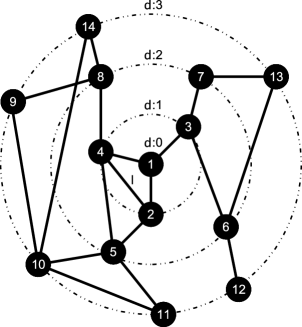
Figure 1: A small network with 3 concentric levels considering node $i$ as reference 

The concept of concentric levels allows the complementation of the traditional measurements, focused not on the local topological properties of nodes, but taking into account its successive neighborhoods. In general, the concentric measurements are calculated considering relationships between the nodes and edges at two or more concentric levels. The following measurements can be naturally generalized for weighted networks by performing some modifications.

The concentric node degree, $k_{d}(i)$, of a reference node $i$ at the concentric level $d$ is defined as corresponding to the number of edges connecting the nodes in $R_{d}(i)$ and $R_{d+1}(i)$. As an example, we have for Figure 1 $k_{0}(1)=3$, $k_{1}(1)=5$ and $k_{2}(1)=7$. Note that the concentric node degree is not an average value taken among the number of nodes in $R_{d}(i)$. This measurement is the direct extension of the well known node degree where the reference node is understood as the nodes inside the ball $B_{d}(i)$ (i.e. the ball containing the nodes in rings $0$ to $d$). The concentric node degree can be extended for weighted networks by taking the sum of the weight values for every connection between these nodes and the nodes at the next level.

The concentric clustering coefficient, $cc_{d}(i)$, is the immediate generalization of the traditional clustering coefficient and considers the only the nodes and connections of the ring $R_{d}(i)$. It is defined as in Equation 3, where the number of edges in $R_{d}(i)$ is expressed as $e_{d}(i)$, and the number of elements is represented as $n_{d}(i)$.

$$cc_{d}(i)=2\frac{e_{d}(i)}{n_{d}(i)(n_{d}(i)-1)}$$ (3)

For node $i=1$ in the network shown in Figure 1, we have that $cc_{1}(1)=1/3$, $cc_{2}(1)=0$, and $cc_{3}(1)=1/5$.

Other interesting concentric measurements which can be obtained with respect to the reference node $i$ and used in order to complete the characterization of complex networks include the following:

Convergence ratio ($C_{d}(i)$): Corresponds to the ratio between the concentric node degree of node $i$ at distance $d$ and the number of nodes in the ring at next ring, i.e.

$$C_{d}(i)=\frac{k_{d}(i)}{n_{d+1}(i)}.$$ (4)

This measurement quantifies the average number of edges received by each node in the ring $d+1$. We have necessarily that $C_{0}(i)=1$ for whatever node selected as the reference $i$. In the case illustrated in Figure 1, we have $C_{0}(1)=1$, $C_{1}(1)=5/4$ and $C_{2}(1)=1$.

Intra-ring degree ($A_{d}(i)$): This measurement is obtained by taking the average among the degrees of the nodes in the subnetwork $\gamma_{d}(i)$. Observe that only those edges between the nodes in such a subnetwork are considered, therefore overlooking the connections established by such nodes within the nodes in the rings at levels $d-1$ and $d+1$. For instance, we have for the situation in Figure 1 that $A_{1}(1)=1/3$, $A_{2}(1)=0$ and $A_{3}(1)=1/2$. For weighted networks the value of intra-ring is the average of the weights of all nodes at the rings $R\{d-1\}$ and $R\{d+1\}$.

Inter-ring degree ($E_{d}(i)$): This measurement corresponds to the average of the number of connections between each node in the ring $R_{d}(i)$ and those in $R_{d+1}(i)$. For instance, for Figure 1 we have $E_{0}(1)=3$, $E_{1}(1)=5/3$ and $E_{2}(1)=3/2$. Observe that $E_{d}(i)=k_{d}(i)/n_{d}(i)$.

concentric common degree ($H_{d}(i)$): Equal to the average node degree among the nodes in $R_{d}(i)$, considering all edges in the original network. For Figure 1 we have $H_{0}(1)=1$, $H_{1}(1)=10/3$ and $H_{2}(1)=16/7$. The concentric common degree expresses the average node degree at each concentric level, indicating how the network node degrees are distributed along the network hierarchies.

Table 1 summarizes the concentric measurements to be used in this paper, all of which are defined with respect to one of the network nodes, identified by $i$, taken as a reference and at a distance $d$ from that node.

$e_{d}(i)$	conc. number of edges among
	the nodes in the ring $R_{d}(i)$
$n_{d}(i)$	conc. number of nodes
	in the ring $R_{d}(i)$
$k_{d}(i)$	concentric degree
	of node $i$ at distance $d$
$A_{d}(i)$	intra-ring node degree
	of node $i$ at distance $d$
$E_{d}(i)$	inter-ring node degree
	of node $i$ at distance $d$
$H_{d}(i)$	concentric common degree
	$i$ of node at distance $d$
$cc_{d}(i)$	conc. clustering coefficient
	of node $i$ at distance $d$
$C_{d}(i)$	convergence rate at
	concentric level $d$

Table 1: The concentric measurements considered in the current article. 

4 Statistical Concepts

Two statistical methodologies are used in the present paper in order to obtain groups of nodes with similar concentric measurements. The first step is to choose a distance measurement [11, 12](i.e. how similar two nodes are, in terms of a set of measurements). Because of the varying forms of the concentric measurement distributions, a non-parametric distance such as the Spearman rank correlation coefficient, should be adopted.

4.1 Spearman Rank Correlation.

The Spearman rank correlation coefficient is a statistical measurement quantifying how strong is the tendency of two random variables to vary together. Unlike the Pearson correlation coefficient, this measurement is not restricted to linear joint variations and can be used to quantify the similarity between the form of two curves (or data sets). In fact, the Spearman rank correlation is a special case of the Pearson correlation, where every value of the curve is ranked before calculating the coefficient.

Given two normalized distributions of two random discrete variables, X and Y, the Pearson correlation coefficient between them is defined by the covariance of those two variables divided by their respective standard deviations, i.e.:

$$r_{XY}=\frac{cov(X,Y)}{\sigma_{X}\sigma_{Y}}$$ (5)

Given $n$ samples of the random variables $X$ and $Y$, henceforth expressed $x_{i}$ and $y_{i}$, the respective Pearson Correlation Coefficient can be estimated as:

$$r_{XY}=\frac{\sum(x_{i}-\bar{x})(y_{i}-\bar{y})}{(n-1)\sigma_{X}\sigma_{Y}}$$ (6)

The Spearman rank correlation coefficient $\rho$ can be obtained by replacing $X$ and $Y$ values by their ranked version $X^{*}$ and $Y^{*}$. For example, considering a data set with $X=\{1.1,3,0.5,100\}$ and $Y=\{2,0.8,1,0.1\}$, the ranked data set will be $X^{*}=\{2,3,1,4\}$ $Y^{*}=\{4,2,3,1\}$, and the Spearman rank coefficient will be $\rho=r_{X^{*}Y^{*}}$

5 Methodology

In order to illustrate the use of concentric measurements and node classification, we consider a collaboration network obtained from real data, which will be compared to Barabasi-Albert(BA) and Erdös and Rényi(ER) counterparts.

The collaboration network, presented in this work for the first time, was created by collecting data about co-authorship in published articles, where each node represents an author and each undirected edge represents a paper written by the respective two nodes (authors). Because of the possible existence of more than one paper by the same two authors, those edges are weighted with values representing the number of papers that those authors wrote together. This network was obtained from the library database of ”Universidade de São Paulo”. In addition to the collaborative information, every node was labeled with the author corresponding department. The network resulted with 5630 nodes and an average topological node degree of $\left<k_{t}\right>\approx 15$ and average strength of $\left<k\right>\approx 40$ .

The simulated networks, of type BA and ER, were obtained by the classical methods [3]. Random networks(ER) were generated by selecting edges with uniform probability $p$, while the BA networks were grown by starting with $m0$ randomly interconnected nodes and adding new nodes with $m$ edges which are attached to the existing nodes with probability proportional to their respective node degrees. The networks were created with 5000 nodes and average node degree of $\left<k\right>\approx 16$ for BA and $\left<k\right>\approx 15$ for ER.

We started the analysis of the characteristics of the real and theoretical networks by considering the traditional node degree. Next, a collection of concentric measurements were obtained for all the networks, considering every node of as the center (reference), and then taking the average values and average $\pm$ standard deviations. The considered measurements were the concentric node degree, concentric clustering coefficient, intra-ring degree, inter-ring degree, common node degree and convergence ratio. The distributions of such measurements obtained for the three networks were compared as discussed in the next section.

While distributions of the concentric measurements supply subsidies for a global characterization of the networks, they do not convey information about the individual node concentric characteristics. This information can be obtained in terms of the individual node concentric measurements among the several levels centered at this node. In order to classify those nodes into groups with similar concentric features, the agglomerative hierarchical clustering algorithm, using spearman rank coefficient as distance measure, was applied over the individual node concentric clustering coefficients and convergence ratios. This data was obtained only for the collaboration network. The resulting tree (called dendogram) was truncated so as to yield eight groups of nodes with similar properties.

Because the nodes in collaborative network are labeled with the respective department of the corresponding author, the effectiveness in the segregation of those groups can be quantified in the sense of the percentage of nodes common to departments and communities.

6 Results and Discussions

This section begins by presenting the results obtained for the concentric level measurements described in the methodology section and then discusses such results while comparing the collaborative network with the other two models. Finally, the agglomerative concentric clustering results are shown as dendograms and average concentric measurements distributions obtained for each group. The effectiveness of the segregation of labeled groups is presented in the form of pie charts.

By obtaining the traditional degree distribution of the considered networks, as can be seen in the loglog curves of Figure  2, the collaboration network (a) can be understood as a scale-free network, like the BA model (b), because of the well-known power law behavior of those curves. It is interesting to note that the power coefficients of the two scale free networks are distinct.

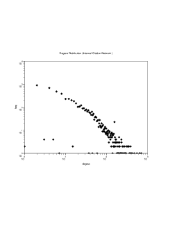
(a)

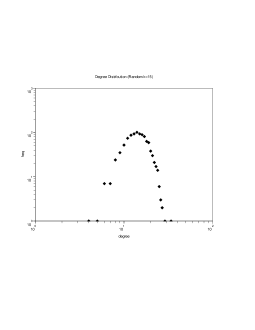
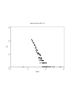
(b)	(c)

Figure 2: Average degree distributions for the three considered networks: (a)Collaborative network, (b) random ER model and (c) Barabási-Albert BA model. ER and BA networks with average degree $\left<k\right>=4$.  

Figures 3 to 9 present the concentric measurements distributions obtained for the three networks while considering all the nodes. The asterisks indicate the position of the average shortest path between any pair of nodes, which are included in order to provide a reference for the hierarchical analysis.

Figure 3 shows the concentric number of nodes (average $\pm$ standard deviation) obtained for the considered networks. All curves are characterized by a peak. Interestingly, the collaboration network presents a considerably smoother curve and wide peak when compared with the simulated models. In addition, its high values of standard deviation suggest a wide variation of concentric features among the nodes. The values of concentric node degrees, shown in Figure 4, are similar to the respective measurements of the concentric number of nodes.

Figure 3: Hierarchical number of nodes (average $\pm$ standard deviation) for all considered networks, which are identified above each graph. Observe that most curves are characterized by a peak. The average value of the shortest path between any two nodes is marked by an asterisk.  

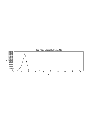
Figure 4: Hierarchical node degrees obtained for all the considered network models. The curves are similar to those obtained for the concentric number of nodes, except for a expected offset at one level. 

The inter-ring degree curves, shown in Figure 5, are monotonically decreasing after the first ring. While such curves for the BA and ER model are clearly distinct, the curve for the collaborative network shows a mix of both behavior. The collaborative network curve begins with a constant value, like for the ER model, and then decreases in a smooth fashion, like the curve for the BA model. The curves obtained for the BA case show a peak at the first ring, which is a consequence of the high chance of finding a hub at that level. However, that characteristic seems not to be present on the collaborative network. An explanation for this effect is that the average topological distribution of hubs in the collaborative network and BA model are very different.

Figure 5: Inter ring degree values for the considered network models. 

The results for intra-ring degree, shown in Figure 6, are very similar to the concentric number of nodes measurement, characterized by a peak, except for the collaborative network, which presents a wider peak centered at the left hand side of the graph.

Figure 6: Intra Ring Degree values for the considered network models. 

Figure 7 shows the values of concentric common degree for the considered networks. These distributions are characterized by a decreasing curve starting at the first level. Generally, these curves are similar to those obtained for the inter-ring degrees, except that the present curves are wider and the collaborative network has a well defined peak at first level. Another observation is that the average concentric common degree tends to be higher at the initial concentric levels, which is a consequence of the fact that the largest hubs present in the BA model tend to be reached sooner, providing bypasses to the other nodes and therefore left-shifting the the peak and reducing the number of concentric levels. This is the main reason why the peak in the BA networks tends to be displaced to the lefthand side than in the random network. As with the inter-ring degree, the distribution of concentric degree for the collaborative network results in a mix of the characteristics of the curves for both models, supporting the evidence that the topological location of the hubs tends to be more widespread than those in the BA model.

Figure 7: Hierarchical common degree measurements with the respective $\pm$ standard deviations obtained for the considered models. 

Figure 8: Hierarchical clustering coefficient degree measurements. Note the higher values of standard deviation when compared to those in the other measurements. 

As shown in Figure  8, the concentric clustering coefficients curves are very distinct among both simulated models. The curves for the ER model present a fast increase in value, followed by a plateaux and then a rapid decrease. In fact, the nodes at each ring of those networks are characterized by low interconnectivity. The concentric clustering coefficient curves obtained for the BA and the collaborative network, present much higher values and involve a sharper peak. In addition, the curve for the co-authorship network tends to present another peak along the last levels.

The convergence ratios obtained for each of the considered network models, shown in Figure 9, yielded the most distinct curves among the simulated models and collaborative network. The curves for the BA and ER models are characterized by similar behavior among themselves and a peak at the last levels (except for the regular models), along which the concentric expansion tends to saturate, i.e. after the peak is reached. Note also that sharper peaks tend to be obtained for high values of $k$. The collaborative curve presents a wider peak, with the center displaced to the lefthand side, far away from the average shortest path. This is a consequence of the fact that, differently of what is obtained for the BA, the hubs are reached gradually along the concentric levels while starting from most nodes.

Indeed, as verified experimentally in [10], the position and width of the peak of the convergence ratio is ultimately defined by the distribution of hubs along the hierarchies.

The fact that the convergence ratios obtained for the co-authoship networks, shown in Figure 9, tended to be relatively uniform along the hierarchies indicates that the hubs are not highly interconnected. In other words, the hubs tend to cover different portions of the network. If we understand that the hubs are more likely to correspond to leader scientists, it can be inferred from the convergence ratios results that the multidisciplinarity would be ultimately implemented by the respective co-authors connected to each hub.

Figure 9: Convergence Ratio measurements for the considered networks. 

Among all the considered measurements, the concentric common degrees and concentric clustering coefficients were found to provide the most distinct curves for each network, revealing more information about the distribution of hubs and the interconnectivity along the concentric levels. Because the collaborative network curves have the highest values of standard deviation, their individual nodes may have distinct concentric features, and can be grouped into clusters of similar features. The remainder of this section presents the results obtained by application of an agglomerative hierarchical clustering algorithm using the data obtained by the concentric clustering coefficient and convergence ratios. The following graphs were obtained, showing the average $\pm$ standard deviation of the concentric measurements obtained at each respective level in the dendrograms. Starting at the right hand side of the tree, the nodes are progressively merged with basis on the similarity of their concentric clustering coefficients, yielding the taxonomical categorization of the nodes into meaningful clusters, identified by each branching point in the tree.

Figure  10 shows the graph for concentric clustering coefficients and the respectively obtained clusters. The mean degree and number of nodes of each cluster are given above each graphic. As can be seen, in the first branch point leading to the first clusters (i.e. B and C), about $17\%$ of nodes of the network are in cluster B and, differently from the curve for all nodes(i.e. A), the clustering coefficient distribution shows only a peak, reveling that those nodes have distinct hierarchical behavior when compared with those from cluster C. Note that cluster B leads to a great variety of types of curves, while the curve for cluster H has a peak centered at the concentric level 2, those for cluster I are centered at level 1. Cluster E shows that about 25 nodes have very specific distribution including two peaks centered at levels 1 and 2 (as in J) or two peaks centered at levels 2 and 3 (as in K). The branch corresponding to cluster C shows two basic structures (G and F), both including the second peak, but the first one is wider for the cluster G when compared with F.

The results obtained for the convergence ratio can be seen in Figure 11. The main distinction between the final groups are the positions of the center of the peak for each curve, varying from peaks centered at the concentric level 4 — as in cluster K, to around level 8 — as in M. In the case of the convergence ratio, the displacement indicates how close the groups of nodes are to the hubs.

Because every node in the collaborative network are labeled with the author department, the percentage of nodes belonging to each department is given by each obtained group. The results can be seen in Figures  12 and  13 for concentric clustering coefficient and convergence ratio, respectively. Only the seven most representative departments of a cluster are shown, other departments are merged into a single section of the pie chart. Note that the most representative clusters for department segregation are located in the second blanch points.

Figure 10: Graphs of the average $\pm$ standard deviation of the concentric clustering coefficient obtained for the co-authorship network. Only four levels of the dendogram obtained by the agglomerative hierarchical clustering are shown. 

Figure 11: Graphs of the average $\pm$ standard deviation of the concentric convergence ratio obtained for the co-authorship network. Only four levels of the dendogram obtained by the agglomerative hierarchical clustering are shown. 

Figure 12: Pie charts with the percentage of nodes in each department for each cluster obtained by using the Clustering Coefficient.

Figure 13: Pie charts with the percentage of nodes in each area of knowledge for each cluster obtained by using the Clustering Coefficient.

Figure 12 shows the pie charts of the sets of nodes obtained by hierarchical clustering and considering the clustering coefficient. Each pie chart includes a respective legend showing the most highly represented institutes and their relative percentage considering each level. For example, considering the branching level 1 (i.e. groups D to G), the sum of the percentages of each institute for all pie charts should add to 1. This is the case of the institute H1 at the branching level 1, which presents a participation of $17.1\%$ in pie chart D, $3.2\%$ in chart E and $75.3\%$ in chart G.

For most levels, the pie charts do not present marked homogeneity as far as the nature of the institutes is concerned (i.e. human, exact and biological areas). The departments are namely according its knowledge area followed by a number, where H# stands for human, E# for exact and B# for biological areas. However, we found the remarkable result that a large part of the most representative institutes in chart C were not only from the biological area, but also located in a same city in the countryside of São Paulo State. Therefore, these two factors seem to have implied a distinctive pattern of collaborations. In addition, by taking into account the respective clustering coefficient measurements in Figure 10, it becomes clear that these collaborations involve a peak of clustering coefficient at the hierarchical level 1. This provides further indication that the collaborations in pie chart C indeed takes place at a more localized level, implied by the geographical position of those institutes. This more localized collaboration pattern remains in the next branching, i.e. in pie chart F. The institutes in the sister chart, i.e. G, have a more widespread collaboration pattern as indicated in the wider hierarchical clustering coefficient signature in Figure 10. As far as the subdivision of the chart B is concerned, one of the sister charts (i.e. D) contains a substantially higher overall percentage of institute than the chart E. Therefore, we will not consider the latter and its respective subdivisions J and K in the following discussion. Charts D and E are characterized by the absence of the secondary peak in the clustering coefficient signature (compared to charts F and G). The institutes in chart D are heterogeneous as far as the scientific area is concerned, but are all located in the capital (except for E5).

Figure 13 shows the distribution of the scientific area for each respective pie chart as in Figure 12. Most of the cases in the upper branching (i.e. B, D, E, I, J, K) have a predominance of the human area. Contrariwise, only the cases G, O resulted with predominance of the human area in the lower branch. The biological area is over-represented in the branch C, F, L, M. This is in agreement with the above discussion. The exact area is more uniformly distributed among all cases, predominating only in cases H and N.

7 Concluding Remarks

One of the interesting applications of complex networks has been for the investigation of patterns of authorship and collaborations in scientific production (e.g. [13, 14, 15, 16, 17, 18]). The current work has extended such investigations by considering concentric measurements, which are capable of providing additional information about the connectivity around each node (e.g.[7, 10]), as well as the organization of the results by using pattern recognition methods (more specifically hierarchical clustering). We applied such a methodology to real data related to the scientific collaborations between authors from the several institutes that compose the University of São Paulo (USP). A number of interesting results have been obtained. First, we found that the geographical position of institutes tended to produce well-defined groups, characterized by more localized clustering coefficient. This suggests that the collaborations are more intense about the institutions in the same city. We also found that the three main scientific areas tended to be differently represented in the obtained groups, with the exact sciences tending to appear more uniformly in the majority of groups. This indicates that this area is characterized by a less uniform pattern of collaborations. Future works could address additional measurements and clustering methods, as well as the study of co-authorships with external institutions.

Acknowledgment: Luciano da F. Costa is grateful to FAPESP (05/00587-5) and CNPq (301303/06-1) for financial support. Filipi Nascimento Silva is grateful to CNPq (133256/2007-3) for sponsorship.

References

- [1] P. Erdos and A. Renyi. On random graph i. Publ. Math. Debrecen, 6:290–297, 1959.
- [2] R Albert and AL Barabasi. Statistical mechanics of complex networks. Reviews of Modern Physics, 74:47–97, 2002.
- [3] L. Da F. Costa, F. A. Rodrigues, G. Travieso, and P. R. Villas Boas. Characterization of complex networks: A survey of measurements. Advances In Physics, 56:167–242, 2007.
- [4] MEJ Newman. The structure and function of complex networks. Siam Review, 45:167–256, 2003.
- [5] AL Barabasi and R Albert. Emergence of scaling in random networks. Science, 286:509–512, 1999.
- [6] M. E. J. Newman and E. A. Leicht. Mixture models and exploratory analysis in networks. Proceedings of the National Academy of Sciences of the United States of America, 104:9564–9569, 2007.
- [7] LD Costa. The hierarchical backbone of complex networks. Physical Review Letters, 93, 2004.
- [8] LD Costa and LEC da Rocha. A generalized approach to complex networks. European Physical Journal B, 50:237–242, 2006.
- [9] L. da Fontoura Costa and R. Fernandes Silva Andrade. What are the best concentric descriptors for complex networks? New Journal of Physics, 9(9):2007, 2007.
- [10] Luciano da Fontoura Costa and Filipi Nascimento Silva. Hierarchical characterization of complex networks. Journal of Statistical Physics, 125:845–876, 2006.
- [11] Richard O. Duda, Peter E. Hart, and David G. Stork. Pattern classification. Wiley, New York, 2001.
- [12] Luciano da Fontoura Costa and Roberto Marcondes Cesar Jr. Shape analysis and classification : theory and practice. CRC Press, Boca Raton, FL, 2001.
- [13] MEJ Newman. Scientific collaboration networks. ii. shortest paths, weighted networks, and centrality. Physical Review E, 64, 2001.
- [14] MEJ Newman. Scientific collaboration networks. i. network construction and fundamental results. Physical Review E, 64, 2001.
- [15] MEJ Newman. Coauthorship networks and patterns of scientific collaboration. Proceedings of the National Academy of Sciences of the United States of America, 101:5200–5205, 2004.
- [16] MEJ Newman. The structure of scientific collaboration networks. Proceedings of the National Academy of Sciences of the United States of America, 98:404–409, 2001.
- [17] Alessio Cardillo, Salvatore Scellato, and Vito Latora. A topological analysis of scientific coauthorship networks. Physica A-Statistical Mechanics and Its Applications, 372:333–339, 2006.
- [18] M. E. J. Newman. Who is the best connected scientist? a study of scientific coauthorship networks. to appear in Complex Networks E, Springer, Berlin, 2007.