Area distances of Convex Plane Curves and Improper Affine Spheres

Abstract

The area distance to a convex plane curve is an important concept in computer vision. In this paper we describe a strong link between area distances and improper affine spheres. This link makes possible a better understanding of both theories. The concepts of the theory of affine spheres lead to a new definition of an area distance on the outer part of a convex plane arc. Also, based on the theory of discrete affine spheres, we propose fast algorithms to compute the area distances. On the other hand, area distances provide a good geometrical understanding of improper affine spheres.
Keywords: Area distances, Improper Affine Spheres, Discrete Affine Spheres.

1 Introduction

The area distance of convex plane curves is an important concept in computer vision. These distances can be useful in matching two images of the same object obtained from different points of view [7]. It can also be seen as an erosion, a basic concept of mathematical morphology ([6]).

Improper affine spheres are surfaces in $R^{3}$ whose affine normals at all points are parallel. In this paper, we point out the strong connection between these area distances and improper affine spheres. This connection is used in the development of the theory of area distances: based on the theory of affine spheres, we propose a new definition of area distance on the outer part of a convex curve and new algorithms for computing these distances. This link is also interesting from the point of view of the theory of improper affine spheres, since it provides a geometrical interpretation of them.

Let us make this connection more precise: we first remark that the area distance $f$ to a convex plane curve satisfies the Monge-Ampère differential equation $det(D^{2}(f))=-1$ with boundary conditions $f=0$ and $\nabla(f)=0$ (see [8]). We show in this paper that the graph of $f$ is an indefinite improper affine sphere, with strictly positive Pick invariant. On the other hand, we show also that, at least locally, any indefinite improper affine sphere is an area distance.

For the outer part of the convex curve, we propose to define an area based distance by the Monge-Ampère differential equation $det(D^{2}(f))=+1$ with boundary conditions $f=0$ and $\nabla(f)=0$. Then the graph of $f$ is a definite improper affine sphere, also with strictly positive Pick invariant. We consider in this paper the case of an initial analytic curve. In this case, it is possible to find explicitly a solution to the Monge-Ampère equation, and also to describe its geometrical properties.

Consider now a convex polygon as a discretization of the convex curve. By following the asymptotic lines, we propose a fast evolution algorithm that computes exactly the area distance. We also show that this exact area distance defines a discrete indefinite improper affine sphere, as defined in [5]. We remark that the method proposed in this paper differs completely from that of [9], since the latter considers curves defined in implicit form. For the outer part of the polygon, we also propose a fast evolution algorithm that computes a new distance. This graph of this new distance has the remarkable property of being a discrete definite improper affine sphere, as defined in [5].

In this context, there is a natural duality between points in the inner and the outer part of the convex curve. An interesting fact is that, although this duality is not area preserving, it preserves the measure $J^{1/3}dxdy$, where $J$ denotes the Pick invariant of the corresponding graph. From the discrete point of view, it is interesting to observe that a mesh with planar crosses in the inner part of the curve changes smoothly along the curve to a mesh with planar quadrilaterals in the outer part.

This paper is organized as follows: In section 2, we review the basic concepts related to improper affine spheres, both smooth and discrete. In section 3, we review the definition of area distance in the inner part of a curve and show its strong link with indefinite improper affine spheres. In section 4, we propose the new definition of area distance in the outer part of the curve, show that its graph is an definite improper affine sphere and describe the duality between the inner and the outer area distances.

Notation. For three vectors $X,Y$ and $Z$ in the space, denote by $[X,Y,Z]$ the determinant of the $3\times 3$ matrix whose columns are the vectors $X,Y$ and $Z$. For two vectors $X$ and $Y$ in the plane, denote by $[X,Y]$ the determinant of the $2\times 2$ matrix whose columns are the vectors $X$ and $Y$. Also, denote by $X^{t}$ the transpose of the matrix $X$ and by $R$ the ninety degrees rotation in the anti-clockwise direction. Observe that $[X,Y]=-X^{t}\cdot R\cdot Y$.

2 Improper affine spheres

2.1 Basics

For a surface $S$ parameterized by $q(u,v)=(x(u,v),y(u,v),z(u,v))$ let $L=[q_{u},q_{v},q_{uu}]$, $M=[q_{u},q_{v},q_{uv}]$ and $N=[q_{u},q_{v},q_{vv}]$. We say that $S$ is non-degenerate if $LN-M^{2}\neq 0$. For a non-degenerate surface, the Blaschke metric is given by

$$\phi=\frac{Ldu^{2}+2Mdudv+Ndv^{2}}{|LN-M^{2}|^{1/4}}.$$

It is definite or indefinite according to $LN-M^{2}$ being positive or negative. In the definite case, the affine normal is defined as $\xi=\frac{1}{2}\Delta(q)$, while in the indefinite case $\xi=-\frac{1}{2}\Delta(q)$, where $\Delta(q)$ denotes the laplacian of each coordinate with respect to the Blaschke metric.

An improper affine sphere $S$ is a surface whose affine normals at all points are parallel. We shall assume that the affine normals are parallel to the $z$-axis. Under this hypothesis $S$ is locally the graph of a function $z=f(x,y)$. The following proposition is well-known (see [1]).

Proposition 1

$S$ is an indefinite improper affine sphere if and only if $det(D^{2}(f))=-c$, and a definite improper affine sphere if and only if $det(D^{2}(f))=c$, where $c$ is a positive constant. In both cases, the affine normal is constant and equal to $(0,0,c)$.

In the case $S$ is the graph of $f$, we shall write $q(u,v)=(p(u,v),f(p(u,v)))$. The coefficients of the Blaschke metric can be calculated by the following lemma, whose proof is a straightforward calculation:

Lemma 2

$$\left\{\begin{array}[]{l}L=[p_{u},p_{v}]D^{2}(f)(p_{u},p_{u})\\ M=[p_{u},p_{v}]D^{2}(f)(p_{u},p_{v})\\ N=[p_{u},p_{v}]D^{2}(f)(p_{v},p_{v})\end{array}\ .\right.$$

2.2 Asymptotic and isothermal directions

For an indefinite Blaschke metric, one can find parameters $(u,v)$ such that $L=N=0$. These parameters are called asymptotic parameters and the corresponding tangent vectors are called asymptotic directions. Lines whose tangent vectors are asymptotic directions are called asymptotic lines. Lemma 2 shows that the projections of the asymptotic directions in the $(x,y)$-plane vanish the quadratic form $D^{2}(f)$, and we shall also call them asymptotic directions.

Using asymptotic parameters, the structure equations become

$$\left\{\begin{array}[]{l}q_{uu}=\frac{\omega_{u}}{\omega}q_{u}+\frac{a}{\omega}q_{v}\\ q_{vv}=\frac{b}{\omega}q_{u}+\frac{\omega_{v}}{\omega}q_{v}\\ q_{uv}=-\omega\xi\end{array}\right.$$

where $a_{v}=b_{u}=0$ and $\omega=[q_{u},q_{v},\xi]$. By a good choice of the asymptotic parameters, we can make $a$ and $b$ constants. The Pick invariant is given by $j=\frac{ab}{\omega^{3}}$ (see [4] and [5]). The equations for the planar component are

$$\left\{\begin{array}[]{l}p_{uu}=\frac{\omega_{u}}{\omega}p_{u}+\frac{a}{\omega}p_{v}\\ p_{vv}=\frac{b}{\omega}p_{u}+\frac{\omega_{v}}{\omega}p_{v}\\ p_{uv}=0,\end{array}\right.$$

with $\omega=[p_{u},p_{v}]=-f_{uv}$. From these equations one obtains $[p_{u},p_{uu}]=a$ and $[p_{v},p_{vv}]=-b$. So, if the Pick invariant does not vanish, the planar asymptotic lines are convex.

For a definite Blaschke metric, one can consider also asymptotic parameters, but they are complex ([4]). Consider complex parameters $z=s+it$ and $\overline{z}=s-it$ such that $L(z,\overline{z})=N(z,\overline{z})=0$ and $iM(z,\overline{z})=\Omega^{2}$. Then, in terms of $s$ and $t$, $L(s,t)=N(s,t)=4\Omega^{2}$ and $M(s,t)=0$ ([2]). We call such coordinates isothermal.

In order to differentiate from the indefinite case, we shall use capital letters $P,Q,F,\Omega,A,B$ and $J$ to describe the structure equations, as follows:

$$\left\{\begin{array}[]{l}Q_{zz}=\frac{\Omega_{z}}{\Omega}Q_{z}-\frac{A}{\Omega}Q_{\overline{z}}\\ Q_{\overline{z}\overline{z}}=-\frac{B}{\Omega}Q_{z}+\frac{\Omega_{\overline{z}}}{\Omega}Q_{\overline{z}}\\ Q_{z\overline{z}}=-\Omega\xi\end{array}\right.$$

where $\Omega=-i[Q_{z},Q_{\overline{z}},\xi]$, $A=i[Q_{z},Q_{zz},\xi]$ and $B=-i[Q_{\overline{z}},Q_{\overline{z}\overline{z}},\xi]$. By a good choice of the isothermal parameters, we can make $A$ and $B$ constants. The Pick invariant is given by $J=\frac{AB}{\Omega^{3}}$ (see [2] and [5]). The equations for the planar components are

$$\left\{\begin{array}[]{l}P_{zz}=\frac{\Omega_{z}}{\Omega}P_{z}-\frac{A}{\Omega}P_{\overline{z}}\\ P_{\overline{z}\overline{z}}=-\frac{B}{\Omega}P_{z}+\frac{\Omega_{\overline{z}}}{\Omega}P_{\overline{z}}\\ P_{z\overline{z}}=0,\ \ F_{z\overline{z}}=-\Omega\end{array}\right.$$

with $\Omega=-i[P_{z},P_{\overline{z}}]$. Also $A=i[P_{z},P_{zz}]$ and $B=-i[P_{\overline{z}},P_{\overline{z}\overline{z}}]$.

2.3 Discrete improper affine spheres.

In [2], definitions of discrete proper affine spheres are proposed, both in the indefinite and in the definite case. In [5], these definitions are generalized to discrete improper affine spheres, indefinite and definite. We describe now these latter definitions, with a slight modification in the definite case. Denote by $Z$ the set of integers.

Definition 1

A map $q:Z^{2}\to R^{3}$ is a discrete indefinite improper affine sphere if it has the following properties:

1. For any $(i,j)\in Z^{2}$, the points $q(i,j),q(i+1,j),q(i-1,j),q(i,j-1),q(i,j+1)$ are co-planar.

2. There exists a direction $\xi$ in $R^{3}$ such that, for any $(i,j)\in Z^{2}$, the vector $q(i,j)+q(i+1,j+1)-q(i+1,j)-q(i,j+1)$ is parallel to $\xi$.

Definition 2

A map $Q:Z^{2}\to R^{3}$ is a discrete definite improper affine sphere if it has the following properties:

1. For any $(i,j)\in Z^{2}$, the points $Q(i,j),Q(i+1,j),Q(i,j+1),Q(i+1,j+1)$ are co-planar.

2. There exists a direction $\xi$ in $R^{3}$ such that, for any $(i,j)\in Z^{2}$, the vector $Q(i,j+1)+Q(i,j-1)+Q(i-1,j)+Q(i+1,j)-4Q(i,j)$ is parallel to $\xi$.

3 Inner Area distances

In this section we review some properties of area distances and show the connection between area distances and affine spheres. We show that the graph of an area distance is an indefinite improper affine sphere and that, at least locally, any indefinite improper affine sphere is the graph of an area distance of some convex plane curve.

Moreover, we show that the area distance of polygons define discrete indefinite improper affine spheres and how this fact can be applied to construct a very fast algorithm for computing area distances.

3.1 Definition and properties of the area distance

Consider a smooth convex curve $C$ in the plane without parallel tangent lines. $C$ can have $2$, $1$ or $0$ endpoints. Denote by $D$ the plane region whose boundary is $C$ and the curve(s) obtained from $C$ by a similarity of ratio $\frac{1}{2}$ based at each endpoint of $C$ (see figure 1).

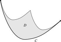
(a) Domain for a curve with 2 endpoints.

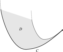
(b) Domain for a curve with 1 endpoint.

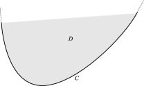
(c) Domain for a curve without endpoints.

Figure 1: Domains for the inner area distance function.

A chord is a line segment connecting $2$ points of $C$. For a point $p\in D$, consider chords $l$ passing through $p$ that, together with $C$, bound regions $D_{l}$. Denote by $l(p)$ the chord such that the area of the corresponding region $D_{l(p)}$ is minimum. The area distance function $f(p)$ is then defined as half of the area of $D_{l(p)}$. Sometimes we shall call this function inner area distance, since in section 4 we shall define another area distance.

Any $p\in D$ is the mean point of the extremities of the chord $l(p)$. This important property was proved first in [6] (see also [7]). Another important property is that $\nabla(f)(p)$ is orthogonal to the chord $l(p)$, with half of the length of it (see figure 2). The third important property is that $det(D^{2}(f)(p))=-1$, for any $p\in D$. This last property was first proved in [8]. The next lemma and proposition describe the $2$ latter properties with more details.

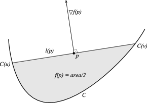
Figure 2: Gradient of the area distance.

Lemma 3

Denote by $C(u(p))$ and $C(v(p))$ the extremities of the chord $l(p)$. Considering $u$ and $v$ as functions of $p$, we have $\nabla(u)=-\frac{2RC^{\prime}(v)}{[C^{\prime}(u),C^{\prime}(v)]}$ and $\nabla(v)=\frac{2RC^{\prime}(u)}{[C^{\prime}(u),C^{\prime}(v)]}$.

Proof. Since $2p=C(u(p))+C(v(p))$, $2I=C^{\prime}(u)\nabla(u)^{t}+C^{\prime}(v)\nabla(v)^{t}$ where $I$ is the identity $2\times 2$ matrix. Multiplying by $C^{\prime}(v)^{t}R$, one obtains the first formula. The second one is analogous.

Proposition 4

The area distance $f$ of a convex arc $C$ satisfies the following formulas:

1. The gradient of $f$ is given by $\nabla(f)=R(\frac{1}{2}(C(v)-C(u)))$.

2. $C^{\prime}(u)$ and $C^{\prime}(v)$ satisfy the equations $D^{2}(f)(C^{\prime}(u),C^{\prime}(u))=0$, $D^{2}(f)(C^{\prime}(v),C^{\prime}(v))=0$ and $D^{2}(f)(C^{\prime}(u),C^{\prime}(v))=[C^{\prime}(u),C^{\prime}(v)]$.

3. $det(D^{2}(f))=-1$.

Proof.

1. By Green’s theorem, one can write $4f(p)=\int_{u}^{v}[C(s)-p,C^{\prime}(s)]ds$. Using the rules for differentiating integrals, one obtains

   $$4\nabla(f)(p)=[C(v)-p,C^{\prime}(v)]\nabla(v)-[C(u)-p,C^{\prime}(u)]\nabla(u)+\int_{u}^{v}RC^{\prime}(s)ds,$$

   $$4\nabla(f)(p)=R(\frac{[C(v)-C(u),C^{\prime}(v)]}{[C^{\prime}(u),C^{\prime}(v)]}C^{\prime}(u)+\frac{[C(v)-C(u),C^{\prime}(u)]}{[C^{\prime}(v),C^{\prime}(u)]}C^{\prime}(v))+R(C(v)-C(u)).$$

   Since, for any $w$, one can write $w=\frac{[C^{\prime}(v),w]}{[C^{\prime}(v),C^{\prime}(u)]}C^{\prime}(u)+\frac{[C^{\prime}(u),w]}{[C^{\prime}(u),C^{\prime}(v)]}C^{\prime}(v)$, we conclude that

   $$\nabla(f)(p)=R(\frac{1}{2}(C(v)-C(u))).$$

2. Differentiating one obtains

   $$2D^{2}(f)=R(C^{\prime}(u)\nabla(u)^{t}-C^{\prime}(v)\nabla(v)^{t}),$$

   and so

   $$D^{2}(f)=\frac{1}{[C^{\prime}(u),C^{\prime}(v)]}\left(RC^{\prime}(u)C^{\prime}(v)^{t}R+RC^{\prime}(v)C^{\prime}(u)^{t}R\right).$$

   One concludes that

   $$C^{\prime}(u)^{t}D^{2}(f)C^{\prime}(u)=C^{\prime}(v)^{t}D^{2}(f)C^{\prime}(v)=0\$$

   and

   $$C^{\prime}(u)^{t}D^{2}(f)C^{\prime}(v)=C^{\prime}(v)^{t}D^{2}(f)C^{\prime}(u)=[C^{\prime}(u),C^{\prime}(v)].$$

3. Since we have assumed that there are no parallel tangents, property 2 guarantees that $D^{2}(f)$ is non-degenerate. Now $C^{\prime}(u)^{t}D^{2}(f)C^{\prime}(u)=0$ implies that $D^{2}(f)C^{\prime}(u)=\lambda RC^{\prime}(u)$, for some $\lambda\neq 0$. And since $C^{\prime}(v)^{t}D^{2}(f)C^{\prime}(u)=[C^{\prime}(u),C^{\prime}(v)]$, $\lambda=1$. So $D^{2}(f)C^{\prime}(u)=RC^{\prime}(u)$ and similarly $D^{2}(f)C^{\prime}(v)=-RC^{\prime}(v)$. Hence $[D^{2}(f)C^{\prime}(u),D^{2}(f)C^{\prime}(v)]=[RC^{\prime}(u),-RC^{\prime}(v)]=-[C^{\prime}(u),C^{\prime}(v)]$, which implies that $det(D^{2}(f))=-1$.

3.2 Area distances as improper affine spheres

3.2.1 Consequences of proposition 4

Proposition 4 implies that the graph of the area distance $f$ to a smooth convex arc $C$ is an indefinite improper affine sphere. Also, the parameterization

$$q(u,v)=(\frac{1}{2}(C(u)+C(v)),f(\frac{1}{2}(C(u)+C(v)))).$$

is asymptotic. Hence $C^{\prime}(u)$ and $C^{\prime}(v)$ are asymptotic directions and the asymptotic lines are obtained from $C$ by similarities of ratio $1/2$. Direct calculations show that $\omega(u,v)=\frac{1}{4}[C^{\prime}(v),C^{\prime}(u)]$. Finally, $f(p)$ represents the area of the region bounded by the two asymptotic lines that start at $p$ and the curve $C$ itself (see figure 3).

If the parameterization of the curve $C$ is by affine arc length, then $a=b=-\frac{1}{4}$. In this case the Pick invariant is $j=4[C^{\prime}(v),C^{\prime}(u)]^{-3}$. Thus it vanishes only at points $p$ such that at least one of the endpoints of minimal chord $l(p)$ belongs to a line segment of the original curve $C$. In particular, if the curve is strictly convex, the Pick invariant never vanishes.

3.2.2 Some explicit formulas for calculating $f$.

By the first item of proposition 4, formulas $f_{u}=f_{x}x_{u}+f_{y}y_{u}$ and $f_{v}=f_{x}x_{v}+f_{y}y_{v}$ imply that

$$f_{u}\left(u,v\right) = \frac{1}{4}\left|\begin{array}[]{cc}x\left(u\right)-x\left(v\right)&x^{\prime}\left(u\right)\\ y\left(u\right)-y\left(v\right)&y^{\prime}\left(u\right)\end{array}\right|$$

$$f_{v}\left(u,v\right) = \frac{1}{4}\left|\begin{array}[]{cc}x\left(u\right)-x\left(v\right)&x^{\prime}\left(v\right)\\ y\left(u\right)-y\left(v\right)&y^{\prime}\left(v\right)\end{array}\right|$$

It is also interesting to consider coordinates $(s,t)$ defined by $2s=u+v$ and $2t=u-v$. In these coordinates, since $g_{s}=g_{u}+g_{v}$ and $g_{t}=g_{u}-g_{v}$, we have

$$f_{s}\left(s,t\right) = \frac{1}{4}\left|\begin{array}[]{cc}x\left(s+t\right)-x\left(s-t\right)&x^{\prime}\left(s+t\right)+x^{\prime}\left(s-t\right)\\ y\left(s+t\right)-y\left(s-t\right)&y^{\prime}\left(s+t\right)+y^{\prime}\left(s-t\right)\end{array}\right|$$ (5)

$$f_{t}\left(s,t\right) = \frac{1}{4}\left|\begin{array}[]{cc}x\left(s+t\right)-x\left(s-t\right)&x^{\prime}\left(s+t\right)-x^{\prime}\left(s-t\right)\\ y\left(s+t\right)-y\left(s-t\right)&y^{\prime}\left(s+t\right)-y^{\prime}\left(s-t\right)\end{array}\right|$$ (8)

3.3 Examples

In this subsection we give explicit examples of area based distance function of convex smooth curves.

Example 1

Consider the parabola parameterized by $C\left(r\right)=\left(r,\frac{r^{2}}{2}\right)$. Integrating $(f_{u},f_{v})=\frac{1}{8}((u-v)^{2},-(u-v)^{2})$ one obtains $f(u,v)=\frac{1}{24}(u-v)^{3}$. Thus a parameterization of the affine sphere in asymptotic coordinates is given by

$$q(u,v)=(\frac{u+v}{2},\frac{u^{2}+v^{2}}{4},\frac{1}{24}(u-v)^{3})$$

with $u>v$. And $\omega(u,v)=\frac{1}{4}(u-v)$. In $(s,t)$ coordinates,

$$q(s,t)=(s,\frac{s^{2}+t^{2}}{2},\frac{t^{3}}{3})$$

and $\omega(s,t)=\frac{1}{2}t$.

Example 2

Consider the circle parameterized by $C(r)=(\cos(r),\sin(r))$. Although this curve admits parallel tangents, the above calculations work well, except at the center of the circle. Integrating $(f_{u},f_{v})=\frac{1}{4}(-\cos\left(u-v\right)+1,\cos\left(u-v\right)-1)$ one obtains $f(u,v)=\frac{1}{4}(u-v-\sin\left(u-v\right))$. Thus a parameterization in asymptotic coordinates is given by

$$q(u,v)=(\frac{1}{2}(\cos(u)+\cos(v)),\frac{1}{2}(\sin(u)+\sin(v)),\frac{1}{4}(u-v-\sin(u-v)))$$

with $u>v$. And $\omega(u,v)=\frac{1}{4}\sin(u-v)$. In $(s,t)$ coordinates,

$$q(s,t)=(\cos(s)\cos(t),\sin(s)\cos(t),\frac{1}{4}(2t-\sin(2t)))$$

and $\omega(s,t)=\frac{1}{4}sin(2t)$.

Example 3

Consider the hyperbola parameterized by $C(r)=(\exp(r),\exp(-r))$. Integrating $(f_{u},f_{v})=\frac{1}{4}(-2+\exp(u-v)+\exp(v-u),2-\exp(u-v)-\exp(v-u))$ one obtains $f(u,v)=\frac{1}{2}(v-u)+\frac{1}{4}(\exp(u-v)-\exp(v-u))$. Thus the asymptotic parameterization is

$$q(u,v)=\frac{1}{2}(\exp(u)+\exp(v),\exp(-u)+\exp(-v),(v-u)+\frac{1}{2}(\exp{(u-v)}-\exp{(v-u)})).$$

with $u>v$. And $\omega(u,v)=\frac{1}{4}(\exp(u-v)-\exp(v-u))$. In $(s,t)$ coordinates,

$$q(s,t)=\frac{1}{2}(\exp(s+t)+\exp(s-t),\exp(-(s+t))+\exp(t-s),-2t+\frac{1}{2}(\exp{(2t)}-\exp{(-2t)})).$$

and $\omega(s,t)=\frac{1}{4}(\exp(2t)-\exp(-2t))$.

Example 4

Consider the cubic parameterized by $C(r)=(r,r^{3})$. Although this is not a convex curve, the above calculations can be done. Integrating the vector field $(f_{u},f_{v})=\frac{1}{4}(2u^{3}-3u^{2}v+v^{3},u^{3}-3uv^{2}+2v^{3})$ one obtains $f(u,v)=\frac{1}{8}\left(u-v\right)^{3}\left(u+v\right)$. Thus the asymptotic parameterization is

$$q(u,v)=\frac{1}{2}((u+v),u^{3}+v^{3},\frac{1}{4}\left(u-v\right)^{3}\left(u+v\right)).$$

with $u>v$. And $\omega(u,v)=\frac{3}{4}(u^{2}-v^{2})$. In $(s,t)$ coordinates,

$$q(s,t)=(s,s(3t^{2}+s^{2}),2t^{3}s)$$

and $\omega(s,t)=3st$.

Example 5

Consider the curve parameterized by $C(r)=(r,r^{4})$. Integrating the vector field $(f_{u},f_{v})=\frac{1}{4}(3u^{4}-4u^{3}v+v^{4},4v^{3}u-3v^{4}-u^{4})$ one obtains $f(u,v)=\frac{1}{4}(\frac{3u^{5}}{5}-\frac{3v^{5}}{5}-u^{4}v+uv^{4})$. Thus the asymptotic parameterization is

$$q(u,v)=\frac{1}{2}(u+v,u^{4}+v^{4},\frac{1}{2}(\frac{3u^{5}}{5}-\frac{3v^{5}}{5}-u^{4}v+uv^{4})).$$

with $u>v$. And $\omega(u,v)=u^{3}-v^{3}$. In $(s,t)$ coordinates,

$$q(s,t)=(s,t^{4}+s^{4}+6s^{2}t^{2},4t^{3}s^{2}+\frac{4t^{5}}{5})$$

and $\omega(s,t)=2t^{3}+6ts^{2}$.

3.4 Local characterization of indefinite improper affine spheres

In this subsection, we show that locally, and up to a constant, any indefinite improper affine sphere with non-zero Pick invariant is the graph of the area distance of a smooth convex plane curve $C$. More precisely, we have the following theorem:

Theorem 5

Let $U$ be an open domain in the $(u,v)$-plane whose closure $\overline{U}$ is contained in the domain of the asymptotic parameterization of an indefinite improper affine sphere $S$. Assume that, restricted to $U$, $S$ is the graph of a function $f(p)$. Then there exists a convex curve $C$ in the plane and a constant $K$ such that $f+K$ is the area distance of $C$.

3.4.1 Some properties of indefinite improper affine spheres

Consider an indefinite improper affine sphere with strictly positive Pick invariant $j$. Assume, w.l.o.g., that the affine normal is $\xi=(0,0,1)$ and consider that $S$ is the graph of a function $f$.

Lemma 6

The following properties hold (see figure 3):

1. We have that $D^{2}(f)(p_{u})=Rp_{u}$ and $D^{2}(f)(p_{v})=-Rp_{v}$.

2. Let $\pi_{1}(p)=p+R\nabla(f)(p)$ and $\pi_{2}(p)=p-R\nabla(f)(p)$. Then $\pi_{1}(p)$ is constant along an asymptotic line $v=v_{0}$ and $\pi_{2}(p)$ is constant along an asymptotic line $u=u_{0}$.

Proof.

1. Since $D^{2}(f)$ is non-degenerate and $D^{2}(f)(p_{u},p_{u})=0$, $D^{2}(f)p_{u}=\lambda Rp_{u}$, for some $\lambda\neq 0$. And since $D^{2}(f)(p_{u},p_{v})=\omega(u,v)=[p_{u},p_{v}]$, $\lambda=1$. A similar reasoning shows that $D^{2}(f)(p_{v})=-Rp_{v}$.

2. Just observe that $p_{u}+RD^{2}(f)p_{u}=0$ and $p_{v}-RD^{2}(f)p_{v}=0$.

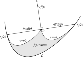
Figure 3: The projections $\pi_{1}$ and $\pi_{2}$.

3.4.2 Proof of theorem 5

Let $\pi_{1}$ and $\pi_{2}$ be the projections defined in lemma 6. We have that $C_{1}=\pi_{1}(\overline{U})$ and $C_{2}=\pi_{2}(\overline{U})$ are compact arcs. It is not difficult to obtain a smooth convex arc $C_{3}$ such that the concatenation $C$ of $C_{1}$, $C_{3}$ and $C_{2}$ is smooth nd convex. Denote by $g$ the area distance function associated to $C$.

One can easily see that $p=\frac{1}{2}(\pi_{1}(p)+\pi_{2}(p))$ and $\nabla(f)(p)=\frac{1}{2}R(\pi_{2}(p)-\pi_{1}(p))$, for any $p\in\overline{U}$. So $\nabla(g)(p)=\nabla(f)(p)$, for any $p\in\overline{U}$. This implies that $f-g$ is constant, which proves the theorem.

3.5 Area distances to polygons

3.5.1 Asymptotic grids 2d and 3d

Let $C$ be a convex polygon with vertices $c_{i}$, $0\leq i\leq N-1$. Denote its sides by the vectors $2L_{i}=c_{i+1}-c_{i}$ and assume that $[L_{i},L_{j}]>0$, for any $j>i$. Assuming $j\geq i$, define the following grid $p\left(i,j\right)$ on the plane by

$$p\left(i,j\right)=\frac{c_{i}+c_{j}}{2}.$$

Note that

$$p\left(i+1,j\right)-p\left(i,j\right)=\frac{c_{i+1}-c_{i}}{2}=2L_{i}=p\left(i+1,j+1\right)-p\left(i,j+1\right),$$

so the grid is formed by parallelograms whose areas will be denoted by

$$a_{ij}=\left[p\left(i+1,j\right)-p\left(i,j\right),p\left(i,j+1\right)-p\left(i,j\right)\right]=\left[L_{i},L_{j}\right].$$

(see figure 4). Define also

$$f\left(i,j\right)=\sum_{i\leq k<l\leq j-1}a_{k,l}=\sum_{i\leq k<l\leq j-1}\left[L_{k},L_{l}\right].$$

Note that $f\left(i,j\right)=0$ if $j=i$ or $j=i+1$.

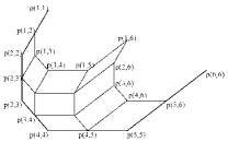
(a) Points and parallelograms.

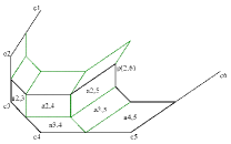
(b) Areas defined by the parallelograms.

Figure 4: Planar mesh of a discrete inner distance.

Proposition 7

The map $q\left(i,j\right)=\left(p\left(i,j\right),f\left(i,j\right)\right)$ is a discrete indefinite improper affine sphere.

Proof.

1. Let

   $$L=\sum_{k=i}^{j-1}L_{k}$$

   Then, since $\left[L_{i},L_{i}\right]=\left[L_{j},L_{j}\right]=0$:

   $$q\left(i,j\right)-q\left(i-1,j\right) = \left(L_{i-1},-\sum_{l=i}^{j-1}\left[L_{i-1},L_{l}\right]\right)=\left(L_{i-1},\left[L,L_{i-1}\right]\right)$$

   $$q\left(i+1,j\right)-q\left(i,j\right) = \left(L_{i},-\sum_{l=i+1}^{j-1}\left[L_{i},L_{l}\right]\right)=\left(L_{i},\left[L,L_{i}\right]\right)$$

   $$q\left(i,j+1\right)-q\left(i,j\right) = \left(L_{j},\sum_{k=i}^{j-1}\left[L_{k},L_{j}\right]\right)=\left(L_{j},\left[L,L_{j}\right]\right)$$

   so whatever linear dependence is satisfied by $L_{i-1}$, $L_{i}$ and $L_{j}$ will also be satisfied by the $z$ coordinates of the three above vectors. This shows that $q\left(i+1,j\right)$ is in the same plane as $q\left(i-1,j\right)$, $q\left(i,j-1\right)$ and $q\left(i,j\right)$. Similarly, one can show that $q\left(i+1,j+1\right)$ is also in this plane (see figure 5).

2. From the equations above, note that

   $$q\left(i+1,j+1\right)-q\left(i,j+1\right) = \left(L_{i},\left[\sum_{k=i}^{j}L_{k},L_{i}\right]\right)$$

   $$q\left(i+1,j\right)-q\left(i,j\right) = \left(L_{i},\left[\sum_{k=i}^{j-1}L_{k},L_{i}\right]\right)$$

   Subtracting,

   $$q\left(i+1,j+1\right)-q\left(i,j+1\right)-q\left(i+1,j\right)+q\left(i,j\right)=\left(0,\left[L_{j},L_{i}\right]\right)=\left(0,-a_{ij}\right)$$

   and hence these vectors are all parallel to the $z$-axis.

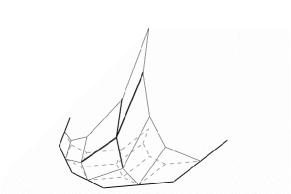
Figure 5: The four line segments in bold are co-planar.

3.5.2 Fast algorithm

Now, if we define the level of a point to be $k=j-i$ we can actually obtain our grid in levels starting from the polygon. At level $0$, $p\left(i,i\right)=c_{i}$ and $f\left(i,i\right)=0$. At level $1$, $p\left(i,i+1\right)=\frac{1}{2}\left(c_{i}+c_{i+1}\right)$ and $f\left(i,i+1\right)=0$. At level $\left(j-i\right)+1$,

$$p\left(i,j+1\right)=p\left(i,j\right)+p\left(i+1,j+1\right)-p\left(i+1,j\right)$$

$$f\left(i,j+1\right)=f\left(i,j\right)+f\left(i+1,j+1\right)-f\left(i+1,j\right)+\left[L_{i},L_{j}\right]$$

This gives us a fast algorithm to calculate all the grid points. In each parallelogram, we can calculate the exact distance by a bilinear interpolation. In figure 6, one can see the result of this algorithm applied to a polygon inscribed in an ellipse.

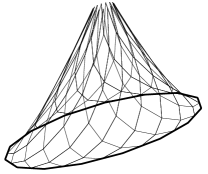
(a) A discrete improper affine sphere.

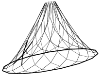
(b) Planar cross in bold.

Figure 6: The inner area distance of a polygon inscribed in a circle.

4 Outer area distances

In this section, we consider the question of extending the area distance to a neighborhood $E$ of $C$ in the outer part of $C$. The idea is to solve the Monge-Ampère differential equation

$$\left\{\begin{array}[]{l}det(D^{2}F)(P)=+1,P\in E\\ \nabla F(P)=0,P\in C\\ F(P)=0,P\in C\end{array}\right.$$

and define the area distance at $P$ by $F(P)$. It is clear that the graph of $F$ defines an improper definite affine sphere.

In this section, we shall first describe a solution to this problem in the case of an analytic curve. Then we prove some properties of this solution, including a relation with the area distance in $D$. Finally, we indicate how to obtain a discrete definite improper affine sphere as an outer area distance of a polygon.

4.1 Definite improper affine spheres from analytic curves

Assume that the parameterization $C(r)=(x(r),y(r))$ is analytic so that we can evaluate its coordinates for complex values of the parameter, $z=s+it$, and $\overline{z}=s-it$. Since $C$ is analytic and real on the real line, the expression $P(z,\overline{z})=\frac{1}{2}(C(z)+C(\overline{z}))$ is real. It represents the planar coordinates of the definite improper affine sphere defined below.

Lemma 8

Consider the inner area function $f$ in coordinates $(s,t)$, and let $F(s,t)=if(s,it)$. Then $F(s,t)$ is real and $\nabla(F)=iR(\frac{C(z)-C(\overline{z})}{2})$.

Proof. From formulas (5) and (8), we can write

$$F_{s}\left(s,t\right) = \frac{i}{4}\left|\begin{array}[]{cc}x\left(z\right)-x\left(\overline{z}\right)&x^{\prime}\left(z\right)+x^{\prime}\left(\overline{z}\right)\\ y\left(z\right)-y\left(\overline{z}\right)&y^{\prime}\left(z\right)+y^{\prime}\left(\overline{z}\right)\end{array}\right|$$ (11)

$$F_{t}\left(s,t\right) = -\frac{1}{4}\left|\begin{array}[]{cc}x\left(z\right)-x\left(\overline{z}\right)&x^{\prime}\left(z\right)-x^{\prime}\left(\overline{z}\right)\\ y\left(z\right)-y\left(\overline{z}\right)&y^{\prime}\left(z\right)-y^{\prime}\left(\overline{z}\right)\end{array}\right|$$ (14)

We conclude that $F(s,t)$ satisfies $F_{s}=F_{x}x_{s}+F_{y}y_{s}$ and $F_{t}=F_{x}x_{t}+F_{y}y_{t}$, where $F_{x}=-\frac{i}{2}(y(z)-y(\overline{z}))$ and $F_{y}=\frac{i}{2}(x(z)-x(\overline{z}))$. Thus $\nabla(F)=iR(\frac{C(z)-C(\overline{z})}{2})$. Observe also that, since $C(z)$ is analytic and real on the real line, $\nabla(F)=\frac{1}{2}iR(C(z)-C(\overline{z}))$ is real. So $F$ is also real.

Proposition 9

The parameterization $Q(s,t)=(P(s+it,s-it),F(s,t))$ is isothermal and defines an improper definite affine sphere $S$. The surface does not depend on the choice of the analytic parameterization of the curve $C$. Also $\Omega(s,t)=-i\omega(s,it)$, $A(s,t)=ia(s,it)$ and $B(s,t)=-ib(s,-it)$. Hence the Pick invariant does not vanish for strictly convex curves $C$.

Proof. Since $\nabla(F)=iR(\frac{1}{2})(C(z)-C(\overline{z}))$, the same proof of proposition 4, item (3), with $(z,\overline{z})$ in place of $(u,v)$ implies that $det(D^{2}(F))=+1$ and that $Q(s,t)$ is an isothermal parameterization of a definite improper affine sphere. If we begin with a different analytic parameterization $C(\psi(z))$, denote by $F_{1}$ the corresponding function. From the above formulas, we have $\nabla(F_{1})(z)=\nabla(F)(\psi(z))\psi^{\prime}(z)$, which implies that $F_{1}(z)=F(\psi(z))$. Thus the surface is independent of the parameterization.

Since $\Omega(z,\overline{z})=\frac{i}{4}[C^{\prime}(z),C^{\prime}({\overline{z}})]=i[P_{z},P_{\overline{z}}]$, we obtain $\Omega(s,t)=\frac{1}{2}[P_{t},P_{s}]$. On the other hand, $\omega(s,t)=\frac{1}{2}[p_{s},p_{t}]$. Thus $\Omega(s,t)=-i\omega(s,it)$.

Finally, $A(s,t)=\frac{i}{4}[C^{\prime}(s+it),C^{\prime\prime}(s+it)]=ia(s,it)$ and $B(s,t)=-\frac{i}{4}[C^{\prime}(s-it),C^{\prime\prime}(s-it)]=-ib(s,-it)$.

4.2 Examples

Given a curve $C$, assume that we can find a parameterization $C(s)=(x(s),y(s))$, with $x(z)$ and $y(z)$ analytic functions.

Example 6

Consider the parabola $C(r)=(r,\frac{r^{2}}{2})$ of example 1. Since $X(z,\overline{z})=\frac{z+\overline{z}}{2}$ and $Y(s,t)=\frac{z^{2}+\overline{z}^{2}}{4}$, we obtain $X(s,t)=s$ and $Y(s,t)=\frac{s^{2}-t^{2}}{2}$. Also, $F(s,t)=if(s,it)=\frac{t^{3}}{3}$. So

$$Q(s,t)=(s,\frac{s^{2}-t^{2}}{2},\frac{t^{3}}{3})$$

$t>0$, defines a definite improper affine sphere. The area element of the Blaschke metric is $\Omega(s,t)=-i\omega(s,it)=\frac{t}{2}$.

Example 7

Consider the circle $C(r)=(\cos(r),\sin(r))$ of example 2. Since $X(z,\overline{z})=\frac{\cos(z)+\cos(\overline{z})}{2}$ and $Y(z,\overline{z})=\frac{\sin(z)+\sin(\overline{z})}{2}$, we obtain $X(s,t)=\cos(s)\cosh(t)$ and $Y(s,t)=\sin(s)\cosh(t)$. Also $F(s,t)=if(s,it)=\frac{1}{2}(\frac{\sinh(2t)}{2}-t)$. Hence

$$Q(s,t)=(\cos(s)\cosh(t),\sin(s)\cosh(t),\frac{1}{2}(\frac{\sinh(2t)}{2}-t))$$

$t>0$, defines a definite improper affine sphere. The area element of the Blaschke metric is $\Omega(s,t)=-i\omega(s,it)=\frac{\sinh(t)\cosh(t)}{2}$.

Example 8

Consider the hyperbola $C(r)=(\exp(r),\exp(-r))$ of example 3. Since $X(z,\overline{z})=\frac{\exp(z)+\exp(\overline{z})}{2}$ and $Y(z,\overline{z})=\frac{\exp(-z)+\exp(-\overline{z})}{2}$, we obtain $X(s,t)=\exp(s)\cos(t)$ and $Y(s,t)=\exp(-s)\cos(t)$. Also, $F(s,t)=if(s,it)=t-\frac{\sin(2t)}{2}$. Hence

$$Q(s,t)=(\exp(s)\cos(t),\exp(-s)\cos(t),t-\frac{\sin(2t)}{2})$$

with $t>0$, defines a definite improper affine sphere. The area element of the Blaschke metric is given by $\Omega(s,t)=\frac{\sin(2t)}{2}$.

Example 9

Consider the cubic $C(r)=(r,r^{3})$ of example 4. Since $X(z,\overline{z})=\frac{1}{2}(z+\overline{z})$ and $Y(z,\overline{z})=\frac{1}{2}(z^{3}+\overline{z}^{3})$, we obtain $X(s,t)=s$, $Y(s,t)=s^{3}-3st^{2}$. Also $F(s,t)=if(s,it)=2t^{3}s$. Hence

$$Q(s,t)=(s,s^{3}-3st^{2},2t^{3}s)$$

$t>0$, defines a definite improper affine sphere. The area element of the Blaschke metric is $\Omega(s,t)=-i\omega(s,it)=3st$.

Example 10

Consider the curve $C(r)=(r,r^{4})$ of example 5. Since $X(z,\overline{z})=\frac{z+\overline{z}}{2}$ and $Y(z,\overline{z})=\frac{z^{4}+\overline{z}^{4}}{2}$, we obtain $X(s,t)=s$ and $Y(s,t)=s^{4}-6s^{2}t^{2}+t^{4}$. Also $F(s,t)=if(s,it)=4s^{2}t^{3}-\frac{4}{5}t^{5}$. Hence

$$Q(s,t)=(s,s^{4}-6s^{2}t^{2}+t^{4},4s^{2}t^{3}-\frac{4}{5}t^{5})$$

$t>0$, defines a definite improper affine sphere. The area element of the Blaschke metric is $\Omega(s,t)=-i\omega(s,t)=6s^{2}t-2t^{3}$.

4.3 Isothermal tangent lines to the curve

4.3.1 Another change of variables

Consider new coordinates $(u,v)$ defined by $s+t=u$ and $s-t=v$.

Lemma 10

Fix a point $P(u_{0},v_{0})$, $u_{0}>v_{0}$ and consider the lines $P(u,v_{0})$, $v_{0}\leq u\leq u_{0}$ and $P(u_{0},v)$, $v_{0}\leq v\leq u_{0}$. These lines touches tangentially the curve at the points $P(v_{0},v_{0})$ and $P(u_{0},u_{0})$, respectively.

Proof. Straightforward calculations shows that

$$P_{u}=\frac{1}{4}((1+i)C^{\prime}(z)+(1-i)C^{\prime}(\overline{z}))$$

and

$$P_{v}=\frac{1}{4}((1-i)C^{\prime}(z)+(1+i)C^{\prime}(\overline{z}))\ .$$

Thus, at $P(u_{0},u_{0})$, $P_{v}=\frac{C^{\prime}(u_{0})}{2}$. Similarly, at $P(v_{0},v_{0})$, $P_{u}=\frac{C^{\prime}(v_{0})}{2}$.

We shall call the above lines the isothermal tangent lines. It is interesting to observe that in the case of a parabola, these isothermal tangent lines are in fact straight lines (see example 6). Also, in examples 6, 7, 8 and 9, the isothermal lines starting at a point $P(u_{0},v_{0})$ do not meet $C$ before the tangency points $P(u_{0},u_{0})$ and $P(v_{0},v_{0})$. We shall refer to this property as non-crossing isothermal tangents. Example 10 does not have this property, i.e., the isothermal tangent lines meet $C$ before they arrive at the tangency points.

4.3.2 Geometric interpretation of $F$ as an outer area distance

We shall assume from now on that the tangent isothermals are non-crossing. Considering coordinates $(s,t)$, we can define a bijection between the inner and the outer parts of $C$, by corresponding the points $p=p(s,t)$ and $P=P(s,ti)$. This correspondence can be defined more geometrically as follows: For $p\in D$, consider the asymptotic lines that passes through $p$ and denote by $C(u)$ and $C(v)$ the points where they touch tangentially $C$. Consider then the tangent isothermal lines in $E$ that touch tangentially $C$ at $C(u)$ and $C(v)$. The intersection of these lines is $P$ (see figure 7).

Figure 7: The correspondence between $p$ and $P$.

For a point $P=P(u_{0},v_{0})$, denote by $A(P)$ the region bounded by the isothermal tangent lines and the part of the curve $C(r)$ with $v_{0}\leq r\leq u_{0}$ (see figure). Next lemma shows that the area of $A(P)$ is $F(P)/2$. This property justify the name outer area distance for the function $F$.

Lemma 11

Assume that the isothermal tangent lines starting at $P=P(u_{0},v_{0})$ are non-crossing. Then the area of $A(P)$ is $F(P)/2$.

Proof. Straightforward calculations shows that $[P_{u},P_{v}]=\frac{\Omega}{2}$. Thus the area of $A(P)$ is given by half of the integral of $\Omega$ over the triangle $T(u_{0},v_{0})$ whose vertices are $(u_{0},v_{0})$, $(u_{0},u_{0})$ and $(v_{0},v_{0})$. The corresponding inner region $a(p)$ has area equal to the integral of $\omega$ over the same triangle. And we know that this area is equal to $f(p)$. Thus

$$F(P)=if(p)=i\int_{T(u_{0},v_{0})}\omega(u,v)dudv=\int_{T(u_{0},v_{0})}\Omega(u,v)dudv$$

and so the area of $A(P)$ is $F(P)/2$.

4.3.3 Relation between the indefinite and definite affine spheres

Proposition 12

Let $b\subset D$ and $B\subset E$ be corresponding regions. Then

$$\int_{q(b)}j^{1/3}=\int_{Q(B)}J^{1/3}$$

where the integrals are taken with respect to the Berwald-Blaschke metric.

Proof. Remember that $j=ab\omega^{-3}$ and $J=AB\Omega^{-3}$. We can assume w.l.o.g. that the curve $C$ is parameterized by affine arc-length. Then $j=J=1/16$. Up to these constants, the above integrals correspond to the areas, in the $(u,v)$-plane, of the regions that represent $b$ and $B$, respectively. Since, in $(u,v)$ coordinates, both regions are the same, the proposition is proved.

4.4 Discrete outer area distances to polygons

Assume that $C$ is a polygon with vertices $P_{i}=(x_{i},y_{i})$, $1\leq i\leq N$. In order to mimic the continuous case, we must consider that $x$ and $y$ are functions of a variable $u\in Z$ and then extend these functions to discrete complex analytic functions.

There are several definitions of discrete analytic functions. We shall adopt a classical one (see [3], ch.5). Consider $g:Z^{2}\to R$ and $h:(Z^{2})^{*}\to R$, where $(Z^{2})^{*}$ denotes the dual lattice. $g$ and $h$ are complex conjugates if $g(u+1,v)-g(u,v)=h(u+1/2,v+1/2)-h(u+1/2,v-1/2)$ and $g(u,v+1)-g(u,v)=-(h(u+1/2,v+1/2)-h(u-1/2,v+1/2))$, for any $(u,v)\in Z^{2}$. These equations are called discrete Cauchy-Riemann equations, and we say that $g+ih$ is discrete analytic.

Using the above definition, we can extend $x$ and $y$ to discrete analytic functions $X+ih_{1}$ and $Y+ih_{2}$. In fact, these functions are uniquely defined if we consider that $h_{j}(u+1/2,1/2)=-h_{j}(u+1/2,-1/2)$, $j=1,2$. This condition is natural for any analytic function that is real on the real line.

As in the continuous case, we must find $F(u,v),(u,v)\in Z^{2}$ such that $(h_{2},-h_{1})=\nabla(F)$. We write

$$F(u+1,v)-F(u,v)=h_{2}(u+1/2,v+1/2)\cdot(X(u+1,v)-X(u,v))-h_{1}(u+1/2,v+1/2)\cdot(Y(u+1,v)-Y(u,v))$$

and

$$F(u,v+1)-F(u,v)=h_{2}(u+1/2,v+1/2)\cdot(X(u,v+1)-X(u,v))-h_{1}(u+1/2,v+1/2)\cdot(Y(u,v+1)-Y(u,v))$$

and, using the discrete Cauchy-Riemann equations, we obtain

$$F(u+1,v)-F(u,v) = -\left|\begin{array}[]{cc}h_{1}(u+1/2,v-1/2)&h_{1}(u+1/2,v+1/2)\\ h_{2}(u+1/2,v-1/2)&h_{2}(u+1/2,v+1/2)\end{array}\right|$$ (17)

$$F(u,v+1)-F(u,v) = \left|\begin{array}[]{cc}h_{1}(u-1/2,v+1/2)&h_{1}(u+1/2,v+1/2)\\ h_{2}(u-1/2,v+1/2)&h_{2}(u+1/2,v+1/2)\end{array}\right|$$ (20)

In order to simplify notations, we shall denote by $h$ the vector $(h_{1},h_{2})$.

Lemma 13

There exists $F:Z^{2}\to R$ satisfying equations (17) and (20).

Proof. One has to show that the discrete derivative $DFu(v)$ of the right hand of (17) with respect to $v$ is equal to the discrete derivative $DFv(u)$ of the right hand of (20) with respect to $u$. We have

$$DFu(v)=[\begin{array}[]{cc}h(u+1/2,v-1/2)+h(u+1/2,v+3/2)&h(u+1/2,v+1/2)\\ \end{array}]$$

and

$$DFv(u)=[\begin{array}[]{cc}h(u+1/2,v+1/2)&h(u-1/2,v+1/2)+h(u+3/2,v+1/2)\\ \end{array}]$$

Thus $DFv(u)-DFu(v)$ is given by

$$[\begin{array}[]{cc}h(u+1/2,v+1/2)&h(u-1/2,v+1/2)+h(u+3/2,v+1/2)+h(u+1/2,v-1/2)+h(u+1/2,v+3/2)\\ \end{array}]$$

which is equal to zero, since $h_{1}$ and $h_{2}$ are discrete harmonic.

We shall denote $P=(X,Y)$ and $Q=(X,Y,F)$. Also, define the co-normal vector by $\nu=(-h_{2},h_{1},1)=(-\nabla(F),1)$. We can write

$$Q(u+1,v)-Q(u,v) = \nu(u+1/2,v+1/2)\times\nu(u+1/2,v-1/2)$$ (21)

$$Q(u,v+1)-Q(u,v) = -\nu(u+1/2,v+1/2)\times\nu(u-1/2,v+1/2).$$ (22)

It follows directly from these equations that the quadrangles whose vertices are $Q(u,v),Q(u+1,v),Q(u,v+1)$ and $Q(u+1,v+1)$ are planar. In fact, each edge is orthogonal to $\nu(u+1/2,v+1/2)$. Thus $Q(u,v)$ defines a conjugate net (see definition in [3]). Denote by $\Delta(g)=g(u+1,v)+g(u,v+1)+g(u-1,v)+g(u,v-1)-4g(u,v)$ the discrete laplacian of $g$. It is clear that $\Delta(Q)$ is parallel to the $z$-axis. This follows directly from the fact that $X$ and $Y$ are discrete harmonic, i.e., $\Delta(X)=\Delta(Y)=0$. Thus $Q(u,v)$ defines a discrete definite improper affine sphere.

We can also calculate $\Delta(F)$. Denote the vectors $P(u+1,v)-P(u,v),P(u,v+1)-P(u,v),P(u-1,v)-P(u,v)$ and $P(u,v-1)-P(u,v)$ by $v_{1},v_{2},v_{3}$ and $v_{4}$, respectively. Since $P(u,v)$ is discrete harmonic, $v_{1}+v_{2}+v_{3}+v_{4}=0$. And the area $A(u,v)$ of the quadrangle whose vertices are $P(u+1,v),P(u,v+1),P(u-1,v)$ and $P(u,v-1)$ is given by $[v_{3},v_{2}]+[v_{1},v_{4}]$.

Lemma 14

$$\Delta(F)(u,v)=A(u,v)$$

Proof. We take as reference the vector $h=h(u+1/2,v+1/2)$. Then

$$h(u-1/2,v+1/2) = h+v_{2}$$

$$h(u+1/2,v-1/2) = h-v_{1}$$

$$h(u-1/2,v-1/2) = h+v_{2}+v_{3}$$

$$= h-v_{1}-v_{4}$$

So

$$F(u+1,v)-F(u,v) = -[h-v_{1},h]=[v_{1},h]$$

$$F(u,v+1)-F(u,v) = [h+v_{2},h]=[v_{2},h]$$

$$F(u-1,v)-F(u,v) = [h+v_{2}+v_{3},h+v_{2}]=[v_{3},h]+[v_{3},v_{2}]$$

$$F(u,v-1)-F(u,v) = -[h-v_{1}-v_{4},h-v_{1}]=[v_{4},h]+[v_{1},v_{4}]$$

We conclude that

$$F(u+1,v)+F(u-1,v)-2F(u,v)=[v_{3},v_{2}]+[v_{1},v_{4}]=A(u,v),$$

thus proving the lemma.

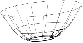
Figure 8: Outer area distance of a polygon inscribed in a circle: observe the planar quadrilateral in bold.

One can see in figure 8 the outer area distance to a polygon inscribed in a circle. In our discrete construction, it is worthwhile to observe an asymptotic net and a conjugate net meeting along a curve. Unfortunately we were not able to give a geometric interpretation of the function $F$ in the discrete case as we have done in the continuous case.

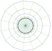
(a) Polygon inscribed in a circle: $(u,v)$ coordinates inside and $(s,t)$ outside.

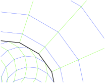
(b) A closer look.

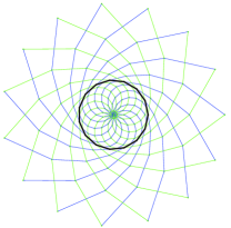
(c) Polygon inscribed in a circle:$(u,v)$ coordinates inside and $(u,v)$ outside.

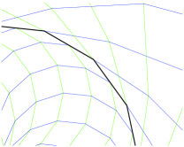
(d) A closer look.

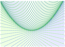
(e) Polygon inscribed in a parabola.

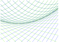
(f) A closer look.

Figure 9: Internal asymptotic and external isothermal lines of polygons.

5 Conclusions

We have shown a very close connection between area based distance, a widely used concept in computer vision, and improper affine spheres. Both theories may take benefit from this connection.

From the point of view of the theory of area based distances, this link allow us to propose a new area based distance outside a convex region and to develop fast algorithms for computing the inner areas.

From the point of view of the theory of improper affine spheres, the approach give a very geometrical description of these surfaces, both in the smooth and in the discrete case.

Acknowledgements. The first author thanks CNPq for financial support through ”Projeto Universal”, 02/2006.

References

- [1] G. Z. An-Min Li, Udo Simon. Global Affine Differential Geometry of Hypersurfaces. De Gruyter Expositions in Mathematics, 1993.
- [2] A. I. Bobenko and W. K. Schief. Affine spheres: Discretization via duality relations. Experimental Mathematics, 8(3):261–280, 1999.
- [3] A. I. Bobenko and Y. B. Suris. Discrete differential geometry: Consistency as integrability. pre-print, 2005.
- [4] S. Buchin. Affine Differential Geometry. Science Press, Beijing, China, Gordon and Breach,Science Publishers, New York, 1983.
- [5] N. Matsuura and H. Urakawa. Discrete improper affine spheres. Journal of Geometry and Physics, 45:164–183, 2003.
- [6] L. Moisan. Affine plane curve evolution: a fully consistent scheme. IEEE Transactions on Image Processing, 7(3):411–420, 1998.
- [7] M. Niethammer, S. Betelu, G. Sapiro, A. Tannenbaum, and P. J. Giblin. Area-based medial axis of planar curves. International Journal of Computer Vision, 60(3):203–224, 2004.
- [8] M. A. Silva. Esqueletos Afins e Equações de Propagação (in portuguese). PhD thesis, Instituto de Matemática Pura e Aplicada - IMPA, 2005.
- [9] M. A. Silva, R. C. Teixeira, S. Pesco, and M. Craizer. A fast marching method for the area based affine distance. Journal of Mathematical Imaging and Vision, to appear.