Comparing and calibrating black hole mass estimators for distant active galactic nuclei
Abstract
Black hole mass (MBH) is a fundamental property of active galactic nuclei (AGNs). In the distant universe, MBH is commonly estimated using the MgII, H, or H emission line widths and the optical/UV continuum or line luminosities, as proxies for the characteristic velocity and size of the broad-line region. Although they all have a common calibration in the local universe, a number of different recipes are currently used in the literature. It is important to verify the relative accuracy and consistency of the recipes, as systematic changes could mimic evolutionary trends when comparing various samples. At , all three lines can be observed at optical wavelengths, providing a unique opportunity to compare different empirical recipes. We use spectra from the Keck Telescope and the Sloan Digital Sky Survey to compare MBH estimators for a sample of nineteen AGNs at this redshift. We compare popular recipes available from the literature, finding that MBH estimates can differ up to dex in the mean (or dex, if the same virial coefficient is adopted). Finally, we provide a set of 30 internally self consistent recipes for determining MBH from a variety of observables. The intrinsic scatter between cross-calibrated recipes is in the range dex. This should be considered as a lower limit to the uncertainty of the MBH estimators.
Subject headings:
black hole physics: accretion — galaxies: active — galaxies: evolution — quasars: general1. Introduction
Understanding the growth of supermassive black holes along with their host galaxies is one of the fundamental questions in current astrophysics (e.g. Di Matteo et al., 2005; Croton et al., 2006). Black hole mass (MBH) is a key parameter in revealing the nature of black hole-galaxy coevolution as well as the physics of active galactic nuclei (AGNs). However, direct mass measurements using the motions of gas and stars in the sphere of influence of a central black hole is limited to very nearby galaxies (e.g. Kormendy & Gebhardt, 2001; Ferrarese & Ford, 2005).
Beyond the very local universe, the so-called “virial” or “empirically calibrated photo-ionization” method based on the reverberation sample is popularly used for active galaxies (e.g. Wandel et al., 1999; Kaspi et al., 2000, 2005; Bentz et al., 2006). This method utilizes broad line widths as velocity indicators and monochromatic continuum or line luminosities as indicators of broad-line region size, hence estimating virial MBH. A combination of the MgII, H, or H broad emission line widths and the 3000Å, 5100Å, H, or H luminosities is typically used, depending on the redshift of the source and the observational setup. Several equations have been presented in the literature to estimate MBH using various combinations of these indicators (e.g., Woo & Urry, 2002a, b; McLure & Jarvis, 2002; Treu et al., 2004; Kollmeier et al., 2006; Greene & Ho, 2005; Vestergaard & Peterson, 2006; Woo et al., 2006; Salviander et al., 2007; Netzer & Trakhtenbrot, 2007; Treu et al., 2007).
Although all three emission lines have a common calibration based on the reverberation sample in the local universe, it is important to verify that different recipes give consistent results; any systematic changes could mimic evolutionary trends given that different recipes are often used in various studies.
At , all three lines can be observed at optical wavelengths, providing a unique opportunity to cross-calibrate the different methods of MBH estimation. Using data from the Keck Telescope and the Sloan Digital Sky Survey for a sample of nineteen AGNs at , we compare the different methods of estimating MBH, and derive a set of self-consistent equations for MBH estimates using every combination of velocity scale (FWHM and line dispersion of MgII, H, or H) and luminosity (3000Å, 5100Å- nuclear and total - H, or H).
The paper is organized as follows. In § 2 we describe the sample selection, observations, and data reduction. In § 3 we describe our line fitting process, based on expansion in Gauss-Hermite series, and the resulting luminosity and width measurements. In § 4 we review the various formulae adopted in the literature, and compare the various MBH estimators. In § 5 we present our self-consistent recipes. Section 6 summarizes our results.
Throughout this paper magnitudes are given in the AB scale. We assume a concordance cosmology with matter and dark energy density , , and Hubble constant H0=70 kms-1Mpc-1.
2. Sample selection, observations and data reduction
The AGN sample was initially selected for stellar velocity dispersion () measurements to measure the MBH- relation at (Treu et al., 2004; Woo et al., 2006). Readers are referred to the papers by Woo et al. (2006) and Treu et al. (2007) – where Keck red spectra (5900Å-7500Å) and Hubble images of the sample were presented – for more details. The relevant properties of the observed objects are listed in Table 1.
High signal-to-noise ratio spectra of nineteen targets were obtained with the Low Resolution Imaging Spectrometer (Oke et al., 1995, hereafter LRIS) at the Keck-I telescope in five runs between March 2003 and July 2005, as detailed by Woo et al. (2006). The red setup is described by Woo et al. (2006). In the blue, the 600 lines mm-1 grism was used, yielding a pixel scale of 0.63Å135 and a resolution of 145 km s-1. Note that objects S16, S31, and S99 included in the papers by Woo et al. (2006) or Treu et al. (2007) lack Keck and/or SDSS spectra and are therefore not considered here.
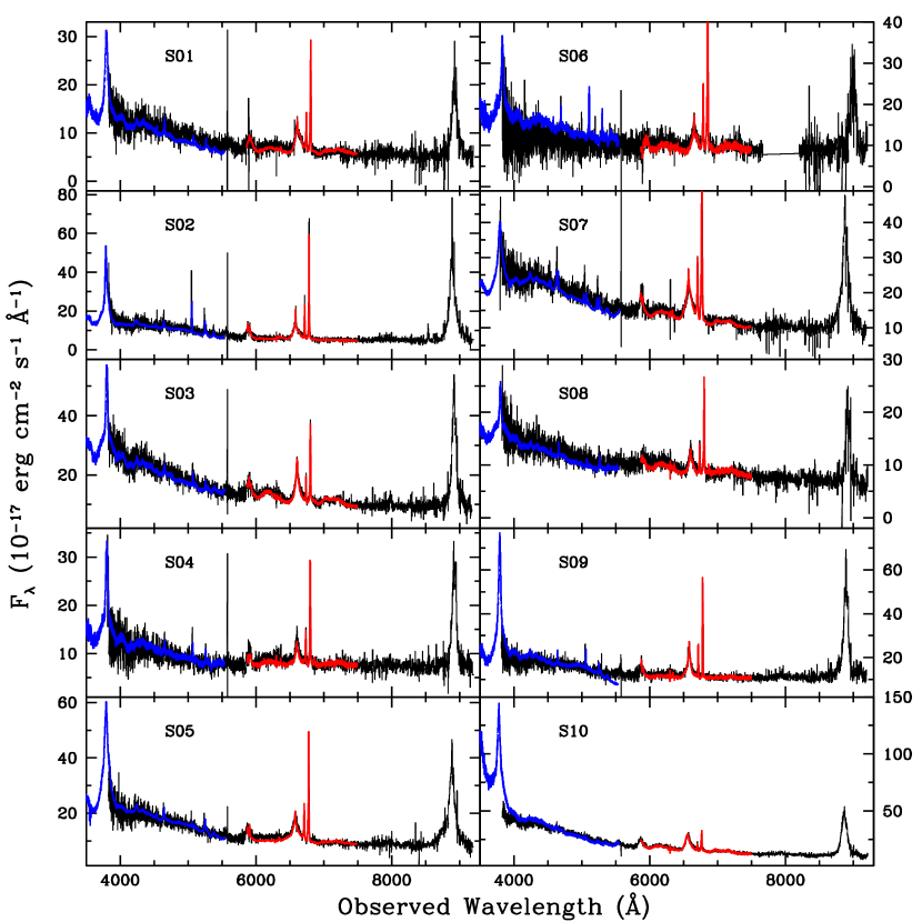
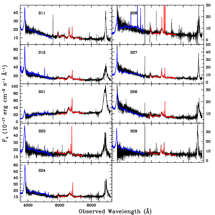
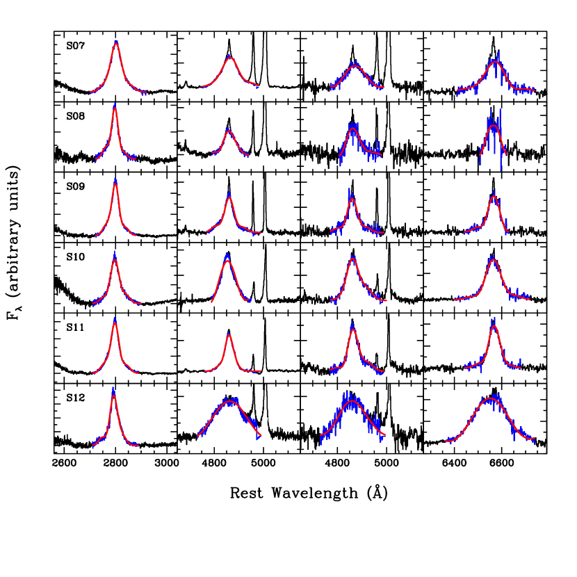
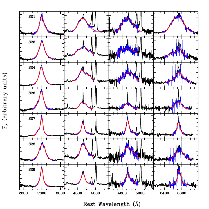
The reduction of the blue spectra was very similar to that of the red spectra described by Woo et al. (2006), except that arc lamp emission lines for Hg and Cd were used for wavelength calibration due to the paucity of sky lines. The flux was calibrated using spectrophotometric stars or A0V type Hipparcos stars. Galactic extinction correction was applied to all data based on the average extinction law derived in Cardelli et al. (1989). The final step in the reduction process involved normalizing all spectra to the proper AB magnitude values from the Sloan photometric database. This was achieved by calculating synthetic and magnitudes from the spectra taking into account the SDSS bandpasses and finding the constant multiplicative factor appropriate to match the SDSS photometry. The final flux-calibrated spectra of all nineteen observed AGNs are shown in Figures 1 and 2.
3. Measurements
The relevant quantities for our purpose are line widths and line and continuum fluxes. In this paper, line widths are measured as FWHM or line dispersion, i.e. the square root of the second central moment:
| (1) |
where Fλ is the flux density, C is the continuum, is the wavelength and is the central wavelength of the line. As described in this section, we derive line widths and fluxes by fitting a Gauss-Hermite series to the data after subtraction of the continuum, Fe emission, and when necessary a narrow component of the line. While the Gauss-Hermite fit is not necessary for the high S/N ratio Keck data – where the quantities can be measured directly from the data (Treu et al., 2004; Woo et al., 2006) – the fitting procedure is needed to obtain robust measurements for the noisier SDSS data. As we demonstrate below by comparing the H measurements from Keck and SDSS data, this fitting procedure gives consistent results between the two datasets, and therefore indicates that the quality of the SDSS data is adequate to measure the width and flux of H and, especially, H, since the latter is considerably stronger.
3.1. Gauss-Hermite Fitting
The emission lines, especially for H, are often asymmetrical, thus making a symmetrical Gaussian approximation of the line profiles undesirable. To account for the asymmetries in the emission lines, we fit a truncated Gauss-Hermite series to the profiles (van der Marel & Franx, 1993). The main advantage of the Gauss-Hermite expansion is that it provides an orthonormal basis set and that the coefficients of the Hermite polynomials (commonly referred to as , , etc.) can be derived by straightforward linear minimization, leaving only two non-linear parameters (the center and the width of the Gaussian). Furthermore, the coefficients can be interpreted in terms of the kinematics of the tracing population (e.g. Gerhard, 1993). The best fit profiles are then used to measure the luminosity, FWHM, and of the emission lines as parameters for the MBH formulae.
We begin the fitting process with continuum subtraction. We identify the continuum level on each side of the three emission lines, using a window of 60 . In the case of MgII, a narrower 40 window is used because the blue continuum of MgII is close to the end of the observed spectral range. For MgII, the ranges typically used are 2660-2700 for the blue continuum level and 2930-2970 for the red continuum level. Similarly for H, the ranges are 4670-4730 Å and 5080-5140 Å for blue and red, respectively, and for H the ranges are 6290-6350 and 6700-6760 . We then independently subtract the continuum by linear interpolation for each line.
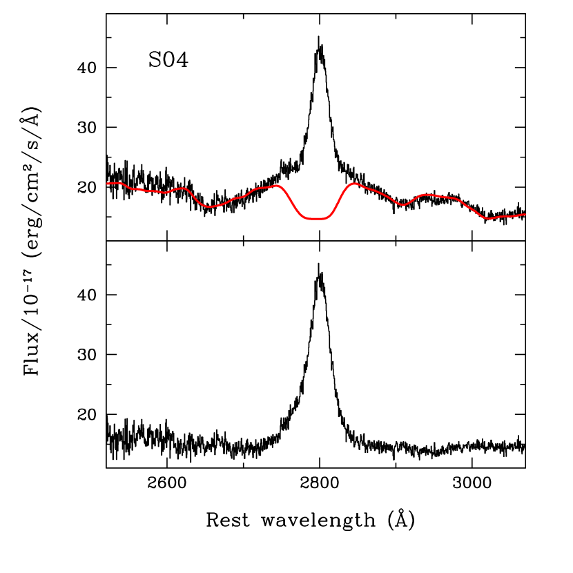
Together with the featureless continuum, we also remove broad nuclear Fe emission underneath MgII and H. For this task we use template spectra of I Zw 1 kindly provided by Todd Boroson and Ross McLure. The procedure is similar to that described by Woo et al. (2006). A typical example of Fe subtraction in the wavelength region around MgII is shown in Figure 3. Removing nuclear Fe emission changes the measured width of H by a negligible amount (the FWHM is unchanged and is reduced by 0.013 dex), but it has a significant effect on MgII (the FWHM is reduced by 0.027 dex, while is reduced by 0.106 dex).
Before fitting the broad lines, we subtract out the narrow lines, extending the procedure described by Woo et al. (2006). For H this involves subtraction of the [OIII] 4959 and 5007 narrow lines, as well as the narrow H line. We subtract [OIII] 5007 directly, and subtract [OIII] 4959 by dividing [OIII] 5007 by 3 and blueshifting. The narrow component of H is subtracted by rescaling and blueshifting [OIII] 5007. The line ratio H / [O III]5007 was allowed to range between 1/20 and the maximum value consistent with the absence of “dips” in the broad component (typically 1/10-1/7; e.g. Marziani et al. 2003). The adopted value of the scale factor is listed in Table 2. The narrow component of H is subtracted by multiplying the determined H narrow component by 3.1 (Malkan, 1983; Osterbrock, 1989) and redshifting.
No attempt is made to remove narrow NII emission lines around H, since they are effectively rejected by the Gauss-Hermite fitting procedure as noise spikes, nor the narrow component (if present) of MgII.
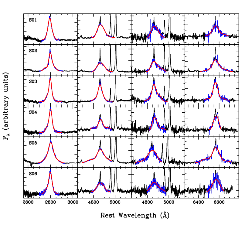
The final step in approximating the line profiles involves fitting the Gauss-Hermite series to the broad lines. The fitting procedure finds the minimum by increasing the order of the Hermite polynomials as required by the data (i.e. only if the goodness of fit, measured by the reduced , improves). Most objects required up to order 6 polynomials (i.e. ) to plateau in reduced . Figures 4 to 6 show our best fits to the MgII, H, and H lines for the nineteen objects. The derived measurements of and FWHM, after removal of the instrumental resolution, are listed in Table 2.
3.2. Luminosities
The formulae for MBH estimates require line luminosities or monochromatic continuum luminosities at given wavelengths. For consistency with Greene & Ho (2005) the line luminosities are calculated from the total flux for the combined broad and narrow components of the H and H emission lines, where the broad component is taken as the best Gauss-Hermite fit, and the narrow component is taken as the appropriately scaled and shifted [OIII] 5007 narrow line (see § 3.1). We note that the narrow components contribute only a small fraction of the total flux of the Balmer lines (e.g., 5% for H – see Table 2, and similarly to H) and therefore they make a contribution of about 0.01 dex to the broad-line size estimates. The H to H flux ratio ranges between 3 and 7 as expected for Seyfert 1s (e.g. Lacy et al., 1982).
The total continuum luminosity at 3000 (5100) is calculated from the average flux in the 2950-3050 (5050-5150) rest frame. In this paper, we use the term total continuum luminosity to indicate the total luminosity as measured within the spectroscopic aperture, i.e. without removing the host galaxy contamination. The fraction of host galaxy contamination depends on the properties of the individual object as well as on the instrumental setup, and it is hence a source of scatter. Nevertheless, the total luminosity is often the only measurement available and therefore it is important to investigate estimators based on this quantity.
The total continuum luminosities at 5100 measured from the SDSS spectra agree to within a few per cent of those inferred from the Keck spectra and those listed in the paper by Woo et al. (2006). By comparing the values listed here with respect to those given by Woo et al. (2006), we infer 0.014 dex as the error on the continuum (L3000 and L5100). For line luminosities, we compare measurements on the fit with measurements on the data, and we take the r.m.s. scatter as the average error. This error is 0.011 and 0.062 dex on LHβ and LHα, respectively. Nuclear luminosities are taken from the HST measurements presented by Treu et al. (2007), except for three objects (S11, S28, and S29), where the nuclear luminosity has been estimated from scaling the total luminosity by the average nuclear fraction for the sample, 0.31. In addition to measurement errors, AGN variability effectively limits the accuracy of the calibration of luminosity-based estimators, to the typical level of variability of 5-10% (e.g., Webb & Malkan, 2000; Woo et al., 2007).

3.3. Line Widths
The MBH estimators depend either on or on the FWHM as a measurement of line width, and hence of the broad line kinematics. Both of these quantities were measured from the Gauss-Hermite fit to the broad lines. Errors on the Keck line width measurements are obtained by comparison with those reported by Woo et al. (2006), which were measured independently and did not rely on Gauss-Hermite expansion. The average error is 0.017 dex for the MgII and H FWHM and . The errors on the SDSS H line width measurements are obtained by comparing the results for H with the Keck fit and assuming that the error is the same for H and H. The average error is 0.051 dex for and 0.040 dex for the FWHM.
The distribution of the FWHM to ratios is shown in Figure 7. The average ratio for H and H is close to the Gaussian value (2.35), although with large scatter, consistent with the sample of Peterson et al. (2004). For MgII the average is considerably smaller indicating significant departure from Gaussianity. A large range of FWHM/ ratios indicates a large scatter between MBH based on FWHM and MBH based on for the sample since velocity is simply derived either from FWHM or by multiplying by a constant as shown in § 4 (see detailed discussion by Collin et al. (2006)).
Figure 8 compares the FWHM of MgII with that of H and H. The FWHM are correlated albeit with substantial scatter. Comparing all the velocity scales, the average ratios and r.m.s. scatters (in parenthesis) are: , , , .
Summarizing these relations, the width of H is generally narrower by 20% than that of H as expected from other studies (e.g. Shuder, 1984; Greene & Ho, 2005), while MgII and H are similar in FWHM but not in . These differences are expected given that different lines trace different species and that their shapes reflect the ionization and excitation variations throughout the region. This finding implies that each line has to be calibrated independently as a velocity estimator and that one cannot go from FWHM to using the simple scaling for a Gaussian distribution. Therefore, we conclude that in general Mg II and Balmer line width cannot be used interchangeably, although in the case of the FWHM of Mg and H the ratio is close to unity (see McLure & Jarvis, 2002; Salviander et al., 2007, for further discussion).
As far as MBH estimators are concerned, the scatter is of order 0.1 dex (i.e. significantly larger than the measurement errors), which sets a lower limit of dex on the relative uncertainty of the cross calibration of simple velocity estimators based on line widths.

4. Review of optical-UV MBH Estimators
We begin this section with a list of the 12 formulae for MBH estimation considered in this paper (§ 4.1). In these formulae, we adopt a notation where Ltotal luminosity at , Lnuclear luminosity at , and L at . All formulae are given in the original notation, without applying any correction for different assumptions on the virial coefficient.
4.1. Summary of existing recipes
McLure & Jarvis (2002), Kollmeier et al. (2006) and Salviander et al. (2007) give equations based on the width of the MgII line and the optical/UV continuum luminosity:
| (2) |
| (3) |
| (4) |
Greene & Ho (2005) and Vestergaard & Peterson (2006) present equations based on the width and luminosities of the H and H broad lines:
| (5) |
| (6) |
| (7) |
Shields et al. (2003), Greene & Ho (2005), Vestergaard & Peterson (2006), Woo et al. (2006), Netzer & Trakhtenbrot (2007), and Treu et al. (2007) adopt the following formulae based on L5100 and the width of the H broad line:
| (8) |
| (9) |
| (10) |
| (11) |
| (12) |
| (13) |
Note that the formulae listed above adopt different estimators of broad-line region velocity ( or FWHM) and size (continuum luminosity or line luminosity).
4.2. Comparison of MBH estimators
In this section we assess the relative consistency of the MBH estimators taken from the literature by comparison with our fiducial black hole mass (as listed in the paper by Treu et al. 2007). The choice of the fiducial estimator is based on reverberation mapping studies of local AGNs, which are mostly based on H and . These studies show that is the most robust velocity estimator (Peterson et al., 2004; Collin et al., 2006). They determine the slope of the size-luminosity relation, taking into account the host galaxy contamination (Bentz et al., 2006), and they set the virial coefficient by requiring that the MBH- relation be the same for active and quiescent galaxies, modulo selection effects (Onken et al., 2004; Lauer et al., 2007).
It is important to notice that the formulae , , , , and have been calibrated on the isotropic spherical virial coefficient (f=3/4 in the notation of Netzer, 1990), and adopt f=1, and , , , , and are based on the recalibration of the virial coefficient given by Onken et al. (2004)111It is also generally assumed that FWHM=2. This is consistent on average with our result for the Balmer lines, albeit with large scatter, but not for the Mg II line.. Therefore, we expect the first set of MBH estimators to give lower values than by dex, and and to give lower values by dex. In the case of and , an isotropic spherical virial coefficient was used. However, their equations were based on a different size-luminosity relation, hence making these formulae approximately equivalent to having the same virial coefficient as , , and (Salviander et al., 2007). As noted by Treu et al. (2007), , , , and agree on average to within a few per cent of . The more discrepant black hole masses are those with different virial coefficients, which can differ on average by as much as dex (i.e. more than a factor of two). Even renormalizing these formulae to the same virial coefficient would still leave discrepancies of order 0.1 dex: after renormalization, and are approximately 0.1 dex larger than while , , and are still 0.1 dex smaller than . This is approximately twice the expected error on the mean given the size of the sample.
These results show that systematic errors as large as dex can be introduced when comparing MBH estimates based on different diagnostics or when comparing AGN MBH estimates to local samples with direct MBH measurements from stellar or gaseous kinematics.
We conclude by discussing the absolute calibration of our fiducial mass estimator. A study by Collin et al. (2006) finds that for the local sample with reverberation based MBH, the widths of the Balmer lines measured on mean spectra are systematically larger than those measured on the r.m.s. spectra for variable objects, suggesting that a smaller virial coefficient than that advocated by Onken et al. (2004) and used for our fiducial mass estimator, should be adopted when measuring widths from mean spectra. This could possibly indicate that our fiducial MBH are overestimated by approximately 0.15 dex. To investigate this effect, in Section 5 we apply our calibrated recipes – based on our fiducial estimator – to the local sample with reverberation based MBH, using published line widths and fluxes measured from single epoch and mean spectra. As discussed in the next section, we find an excellent agreement with the mass inferred from reverberation mapping based on line widths from the r.m.s. spectra, indicating that no such correction is necessary. Data for a larger number of objects with reverberation-based masses are needed to determine the zero point of the virial scalings more accurately, as discussed in the next Section.

5. A set of self-consistent recipes
In this Section we examine all possible combinations of velocity and flux estimators to produce a set of cross calibrated recipes. By comparing with our fiducial mass estimator , we compute the r.m.s. scatter of the residuals to infer a lower limit on the intrinsic uncertainty of each recipe.
In practice, we adopt the following relation:
| (14) |
where is a velocity estimator in units of 1000 km s-1, L is a luminosity estimator in units of 1044 erg s-1 or 1042 erg s-1, respectively for continuum or line luminosity, and we find the that best matches the fiducial estimates. Our range in luminosities is too small to fit for as well, and therefore, we assert the following fiducial values: for L3000, 0.518 for L5100,n, 0.67 for L5100,t, 0.56 for H, and 0.55 for H. These choices are based on the most current calibration of the size-luminosity relation for each wavelength/line. In particular, following the results of the study by Bentz et al. (2006) we adopt 0.518 as the slope of the broad-line region size vs nuclear luminosity relation, while for the size vs total luminosity (i.e. including host galaxy contamination within the spectroscopic aperture) relation we adopt the slope given by Kaspi et al. (2005). Although the former slope is to be preferred when the nuclear luminosity is available, we also provide results for the second slope, which appears to be the best estimate whenever the light from the nucleus and from the host galaxy cannot be disentangled. In general, extrapolations well outside the range considered here are to be done with caution, since most of the local calibrators for the size-luminosity relation are Seyferts and PG quasars in .
We emphasize that this procedure produces self consistent mass estimates, but these all share a common uncertainty in the zero point. In practice, all can be shifted by a constant if it turns out that a different value of the virial coefficient for the local sample of reverberation mapped AGNs is to be preferred. As a sanity check, we applied our calibrated recipes to the local sample with reverberation MBH (Peterson et al. (2004) and recent updates by Bentz et al. (2006), Denney et al. (2006), and Bentz et al. (2007)). Based on the single epoch measurements given by Vestergaard & Peterson (2006) we compared our two estimators based on the FWHM of H, and on L5100,t and H line flux, with the reverberation masses. The agreement is excellent, with average equal to 0.009 dex and 0.023, respectively, with r.m.s. scatter of 0.46 dex and 0.49 dex. Based on the measurements from mean spectra given by Collin et al. (2006) we compared our two estimators based on the FWHM and line dispersion of H, and on L5100,t, with the reverberation masses. The agreement is again excellent, with average equal to 0.004 dex and 0.018, respectively, with r.m.s. scatter of 0.35 and 0.29 dex. The scatter of the difference is combination of effects from uncertainties in time-lag, line width, and luminosity measurements, and scatter in the size-luminosity relation.
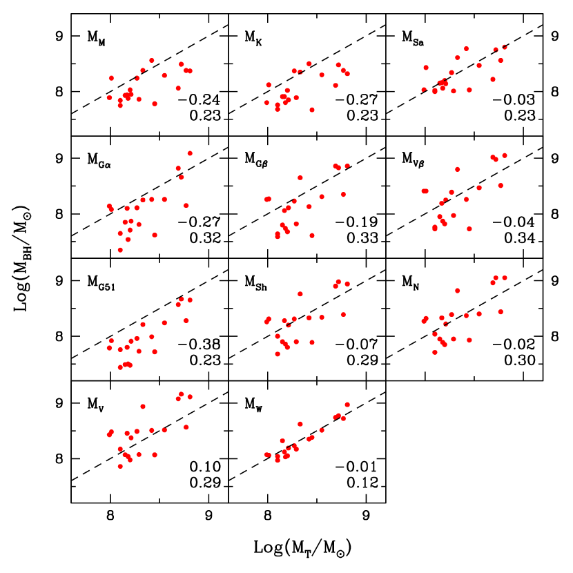
The best fit values of together with the r.m.s. scatter are listed in Table 3. The best fit relations are shown in Figure 10. We note that we included in the recipes the combination of H and L5100,n that was used to compute by Treu et al. (2007). The goal of this exercise is to estimate the measurement errors associated with the relation, given that the input parameters were measured independently for this paper, based on the Gauss-Hermite polynomial expansion fit. Since measurement errors such as narrow line and continuum subtraction dominate over pixel noise, given the high S/N of the Keck data, the r.m.s. of these residuals divided by is effectively the total measurement error, i.e. dex. Thus we can conclude that, for all practical purposes, the r.m.s. scatter that we observe for the other recipes is intrinsic scatter in the relation and not measurement error. This is also the rationale for not showing measurement error bars in the plots.
Looking at Table 3, it appears that the smallest relative scatter is obtained when comparing to black hole masses based on the same velocity scale . This is not surprising, as the velocity scale enters with the square in the MBH estimate and we have seen that velocity scales have typical relative scatter of 0.1 dex. However, the scatter means that adopting optical/UV continuum luminosity as a proxy of the size of the broad-line region introduces an uncertainty of 0.10-0.15 dex in the MBH estimate, with the larger r.m.s. for the line luminosities. The velocity scale that best matches the of H is the line width of MgII, which gives an r.m.s. scatter of 0.17 dex. This is better than the of H (0.20 dex) and the FWHM of H (0.23 dex) – as expected from the large distribution of FWHM/ ratios – which are in turn slightly better than the other indicators. The worst match is obtained for line luminosities with FWHM, with an r.m.s. scatter of dex. From this study, we infer a lower limit to the relative accuracy of the various indicators of order 0.1-0.2 dex, depending on the choice of estimators. If the relationships presented here were to be extended beyond the range of MBH considered, it is likely that the scatter will increase, as suggested by the slope of the points in the corresponding panels. Otherwise, the slope of the size luminosity relation will have to be fitted independently.
6. Summary
In this paper we have used Keck and SDSS spectra of nineteen Seyferts at , to perform a comprehensive study of “virial” black hole mass estimators for broad line AGNs. The main results can be summarized as follows:
-
1.
We have fit Gauss-Hermite series to the data in order to measure the FWHM and of MgII, H , and H , as well as H and H luminosities and continuum luminosities at 3000Å and 5100Å. Measurement errors are approximately 0.02 dex on the MgII and H line widths, 0.04-0.05 on the H line widths, 0.01 dex on the continuum luminosity, 0.01 dex on the H luminosity, and 0.06 dex on the H luminosity.
-
2.
We have compared twelve formulae taken from the literature, showing that MBH estimates can differ systematically by as much as dex (or dex, if the same virial coefficient is adopted). Such differences should be taken into account when comparing data obtained with different methods.
-
3.
We have cross-calibrated a set of 30 empirical recipes based on all combinations of the velocity and luminosity indicators corresponding to the Mg II, H, and H broad lines. Taking the masses measured by Treu et al. (2007) as our fiducial black hole masses, we find that: the absolute scale of the different indicators is calibrated to within 0.05 dex; the best agreement is found when using the line dispersion of H as a velocity estimator, with the residual 0.1 dex r.m.s. scatter resulting from the various continuum luminosity estimators; adopting the line dispersion of Mg II raises the scatter to 0.2 dex; for the other estimators the intrinsic scatter is in the range 0.2-0.38 dex. This implies a lower limit of 0.1-0.2 dex on the validity of each estimator for each individual case.
The newly calibrated recipes should be useful to reduce the sources of systematic uncertainties when comparing different studies.
References
- Bentz et al. (2006) Bentz, M. C., Peterson, B. M., Pogge, R. W., Vestergaard, M., & Onken, C. A. 2006, ApJ, 644, 133
- Bentz et al. (2006) Bentz, M. C., et al. 2006, ApJ, 651, 775
- Bentz et al. (2007) Bentz, M. C., et al. 2007, ApJ, 662, 205
- Cardelli et al. (1989) Cardelli, J. A., Clayton, G. C., & Mathis, J. S. 1989, ApJ, 345, 245
- Collin et al. (2006) Collin, S., Kawaguchi, T., Peterson, B. M., & Vestergaard, M. 2006, A&A, 456, 75
- Croton et al. (2006) Croton, D. J., Springel, V., White, S. D. M., De Lucia, G., Frenk, C. S., Gao, L., Jenkins, A., Kauffmann, G., Navarro, J. F., & Yoshida, N. 2006, MNRAS, 365, 11
- Denney et al. (2006) Denney, K. D., et al. 2006, ApJ, 653, 152
- Di Matteo et al. (2005) Di Matteo, T., Springel, V., & Hernquist, L. 2005, Nature, 433, 604
- Ferrarese & Ford (2005) Ferrarese, L. & Ford, H. 2005, Space Science Reviews, 116, 523
- Gerhard (1993) Gerhard, O. E. 1993, MNRAS, 265, 213
- Greene & Ho (2005) Greene, J. E. & Ho, L. C. 2005, ApJ, 630, 122
- Kaspi et al. (2005) Kaspi, S., Maoz, D., Netzer, H., Peterson, B. M., Vestergaard, M., & Jannuzi, B. T. 2005, ApJ, 629, 61
- Kaspi et al. (2000) Kaspi, S., Smith, P. S., Netzer, H., Maoz, D., Jannuzi, B. T., & Giveon, U. 2000, ApJ, 533, 631
- Kollmeier et al. (2006) Kollmeier, J. A., Onken, C. A., Kochanek, C. S., Gould, A., Weinberg, D. H., Dietrich, M., Cool, R., Dey, A., Eisenstein, D. J., Jannuzi, B. T., Le Floc’h, E., & Stern, D. 2006, ApJ, 648, 128
- Kormendy & Gebhardt (2001) Kormendy, J. & Gebhardt, K. 2001, 586, 363
- Lacy et al. (1982) Lacy, J. H., Malkan, M., Becklin, E. E., Soifer, B. T., Neugebauer, G., Matthews, K., Wu, C.-C., Boggess, A., & Gull, T. R. 1982, ApJ, 256, 75
- Lauer et al. (2007) Lauer, T. R., Tremaine, S., Richstone, D., & Faber, S. M. 2007, ArXiv e-prints, 0705.4103
- Malkan (1983) Malkan, M. A. 1983, ApJ, 264, L1
- McLure & Jarvis (2002) McLure, R. J. & Jarvis, M. J. 2002, MNRAS, 337, 109
- Netzer & Trakhtenbrot (2007) Netzer, H. & Trakhtenbrot, B. 2007, ApJ, 654, 754
- Oke et al. (1995) Oke, J. B., Cohen, J. G., Carr, M., Cromer, J., Dingizian, A., Harris, F. H., Labrecque, S., Lucinio, R., Schaal, W., Epps, H., & Miller, J. 1995, PASP, 107, 375
- Onken et al. (2004) Onken, C. A., Ferrarese, L., Merritt, D., Peterson, B. M., Pogge, R. W., Vestergaard, M., & Wandel, A. 2004, ApJ, 615, 645
- Osterbrock (1989) Osterbrock, D. E. 1989, Astrophysics of gaseous nebulae and active galactic nuclei University Science Books, 1989, 422 p.
- Peterson et al. (2004) Peterson, B. M., Ferrarese, L., Gilbert, K. M., Kaspi, S., Malkan, M. A., Maoz, D., Merritt, D., Netzer, H., Onken, C. A., Pogge, R. W., Vestergaard, M., & Wandel, A. 2004, ApJ, 613, 682
- Salviander et al. (2007) Salviander, S., Shields, G. A., Gebhardt, K., & Bonning, E. W. 2007, ApJ, 662, 131
- Shields et al. (2003) Shields, G. A., Gebhardt, K., Salviander, S., Wills, B. J., Xie, B., Brotherton, M. S., Yuan, J., & Dietrich, M. 2003, ApJ, 583, 124
- Shields et al. (2006) Shields, G. A., Menezes, K. L., Massart, C. A., & Vanden Bout, P. 2006, ApJ, 641, 683
- Shuder (1984) Shuder, J. M. 1984, ApJ, 280, 491
- Treu et al. (2004) Treu, T., Malkan, M. A., & Blandford, R. D. 2004, ApJ, 615, L97
- Treu et al. (2007) Treu, T., Woo, J.-H., Malkan, M. A., & Blandford, R. D. 2007, ApJ, 667, 117
- van der Marel & Franx (1993) van der Marel, R. P. & Franx, M. 1993, ApJ, 407, 525
- Vestergaard & Peterson (2006) Vestergaard, M. & Peterson, B. M. 2006, ApJ, 641, 689
- Wandel et al. (1999) Wandel, A., Peterson, B. M., & Malkan, M. A. 1999, ApJ, 526, 579
- Webb & Malkan (2000) Webb, W. & Malkan, M. 2000, ApJ, 540, 652
- Woo et al. (2006) Woo, J.-H., Treu, T., Malkan, M. A., & Blandford, R. D. 2006, ApJ, 645, 900
- Woo et al. (2007) Woo, J.-H., Treu, T., Malkan, M. A., Ferry, M. A., & Misch, T. 2007, ApJ, 661, 60
- Woo & Urry (2002a) Woo, J.-H. & Urry, C. M. 2002a, ApJ, 579, 530
- Woo & Urry (2002b) —. 2002b, ApJ, 581, L5
| Name | RA (J2000) | DEC (J2000) | z | i’ | |
|---|---|---|---|---|---|
| (1) | (2) | (3) | (4) | (5) | |
| S01 | 15 39 16.23 | +03 23 22.06 | 0.3592 | 18.74 | |
| S02 | 16 11 11.67 | +51 31 31.12 | 0.3544 | 18.94 | |
| S03 | 17 32 03.11 | +61 17 51.96 | 0.3588 | 18.20 | |
| S04 | 21 02 11.51 | -06 46 45.03 | 0.3578 | 18.41 | |
| S05 | 21 04 51.85 | -07 12 09.45 | 0.3530 | 18.35 | |
| S06 | 21 20 34.19 | -06 41 22.24 | 0.3684 | 18.41 | |
| S07 | 23 09 46.14 | +00 00 48.91 | 0.3518 | 18.11 | |
| S08 | 23 59 53.44 | -09 36 55.53 | 0.3585 | 18.43 | |
| S09 | 00 59 16.11 | +15 38 16.08 | 0.3542 | 18.16 | |
| S10 | 01 01 12.07 | -09 45 00.76 | 0.3506 | 17.92 | |
| S11 | 01 07 15.97 | -08 34 29.40 | 0.3557 | 18.34 | |
| S12 | 02 13 40.60 | +13 47 56.06 | 0.3575 | 18.12 | |
| S21 | 11 05 56.18 | +03 12 43.26 | 0.3534 | 17.21 | |
| S23 | 14 00 16.66 | -01 08 22.19 | 0.3510 | 18.08 | |
| S24 | 14 00 34.71 | +00 47 33.48 | 0.3615 | 18.21 | |
| S26 | 15 29 22.26 | +59 28 54.56 | 0.3691 | 18.88 | |
| S27 | 15 36 51.28 | +54 14 42.71 | 0.3667 | 18.80 | |
| S28 | 16 11 56.30 | +45 16 11.04 | 0.3660 | 18.59 | |
| S29 | 21 58 41.93 | -01 15 00.33 | 0.3576 | 18.77 |
Note. — Col. (1): Target ID. Col. (2): RA. Col. (3): DEC. Col. (4): Redshift from SDSS DR4. Col. (5): Extinction corrected AB magnitude from SDSS photometry.
| Name | |||||||||||||
|---|---|---|---|---|---|---|---|---|---|---|---|---|---|
| (1) | (2) | (3) | (4) | (5) | (6) | (7) | (8) | (9) | (10) | (11) | (12) | (13) | (14) |
| S01 | 2260. | 2133. | 1847. | 4418. | 4755. | 3420. | 1.91 | 0.74 | 1.66 | 2.29 | 7.24 | 0.1 | 0.05 |
| S02 | 2914. | 1928. | 2113. | 4000. | 5188. | 3442. | 2.14 | 0.36 | 1.51 | 3.09 | 21.38 | 0.17 | 0.10 |
| S03 | 2147. | 1745. | 1698. | 3345. | 2945. | 2634. | 3.98 | 1.69 | 2.82 | 3.80 | 14.45 | 0.13 | 0.04 |
| S04 | 2253. | 2392. | 983. | 3636. | 3100. | 2617. | 1.86 | 1.42 | 2.24 | 1.35 | 6.92 | 0.08 | 0.06 |
| S05 | 3784. | 3297. | 2686. | 6315. | 5220. | 3751. | 3.39 | 2.04 | 2.75 | 4.37 | 16.60 | 0.11 | 0.05 |
| S06 | 2353. | 1664. | 1382. | 4023. | 4625. | 4306. | 2.75 | 0.54 | 2.69 | 2.00 | 7.94 | 0.1 | 0.13 |
| S07 | 3297. | 2500. | 2531. | 5561. | 4815. | 4326. | 3.72 | 2.26 | 3.02 | 4.90 | 15.14 | 0.1 | 0.06 |
| S08 | 2365. | 1538. | 1015. | 3380. | 3372. | 3017. | 2.29 | 1.25 | 2.57 | 1.12 | 4.47 | 0.1 | 0.08 |
| S09 | 2542. | 2013. | 1462. | 3824. | 2865. | 2710. | 3.16 | 0.78 | 3.09 | 3.80 | 15.49 | 0.11 | 0.04 |
| S10 | 2897. | 1690. | 2056. | 4532. | 4410. | 3498. | 7.08 | 1.11 | 3.80 | 4.79 | 17.78 | 0.11 | 0.02 |
| S11 | 2858. | 1590. | 1435. | 4291. | 2733. | 2569. | 3.24 | 0.88 | 2.45 | 2.75 | 10.72 | 0.08 | 0.01 |
| S12 | 2672. | 3213. | 3232. | 4132. | 9005. | 7163. | 4.37 | 1.05 | 3.24 | 5.01 | 23.99 | 0.06 | 0.02 |
| S21 | 3450. | 3172. | 3208. | 6582. | 7681. | 7493. | 2.69 | 2.30 | 7.24 | 9.12 | 63.10 | 0.07 | 0.03 |
| S23 | 3941. | 3196. | 2688. | 7378. | 9700. | 6870. | 3.09 | 1.20 | 3.55 | 3.47 | 14.13 | 0.1 | 0.05 |
| S24 | 3480. | 2886. | 2667. | 6628. | 7864. | 4468. | 2.82 | 0.44 | 2.95 | 3.47 | 12.59 | 0.1 | 0.04 |
| S26 | 3370. | 1862. | 1657. | 6265. | 5451. | 4440. | 1.78 | 0.50 | 1.58 | 2.69 | 6.46 | 0.07 | 0.12 |
| S27 | 2699. | 1609. | 1157. | 3766. | 2567. | 1832. | 2.19 | 0.92 | 1.82 | 2.45 | 8.32 | 0.17 | 0.05 |
| S28 | 3926. | 2313. | 2221. | 8436. | 5116. | 5412. | 2.45 | 0.76 | 2.29 | 1.91 | 6.61 | 0.09 | 0.03 |
| S29 | 2556. | 1744. | 1520. | 4003. | 3190. | 2216. | 2.09 | 0.59 | 1.74 | 2.04 | 9.12 | 0.1 | 0.05 |
Note. — Col. (1): Target ID. Col. (2): of MgII (km s-1) measured on the line model fit to Keck data. The average error is 0.017 dex. Col. (3): of H (km s-1) measured on the line model fit to Keck data. The average error is 0.017 dex. Col. (4): of H (km s-1) measured on the line model fit to SDSS data. The average error is 0.051 dex. Col. (5): FWHM of MgII (km s-1) measured on the line model fit to Keck data. The average error is 0.017 dex. Col. (6): FWHM of H (km s-1) measured on the line model fit to Keck data. The average error is 0.017 dex. Col. (7): FWHM of H (km s-1) measured on the line model fit to SDSS data. The average error is 0.040 dex. Col. (8): Rest frame luminosity at 3000 in 1044 erg s-1. The average error is 0.014 dex. The actual error will be dominated by variability of order 10%, as for all luminosities listed in this Table. Col. (9): Rest frame nuclear luminosity at 5100 in 1044 erg s-1, from Treu et al. (2007). The average error is 0.08 dex. Col. (10): Rest frame total luminosity at 5100 in 1044 erg s-1. The average error is 0.014 dex. Col. (11): Rest frame H line luminosity in 1042 erg s-1. The average error is 0.011 dex. Col. (12): Rest frame H line luminosity in 1042 erg s-1. The average error is 0.062 dex. Col. (13): Narrow component of H to [OIII]5007 flux ratio. Col. (14): Fraction of flux of the H line in the narrow component.
| (0.47) | (0.518) | (0.69) | (0.56) | (0.55) | |
|---|---|---|---|---|---|
| 7.207 0.052, 0.219 | 7.429 0.039, 0.166 | 7.133 0.045, 0.191 | 7.150 0.053, 0.226 | 6.824 0.051, 0.218 | |
| 7.458 0.027, 0.112 | 7.680 0.021, 0.090 | 7.383 0.028, 0.119 | 7.401 0.038, 0.163 | 7.074 0.042, 0.178 | |
| 7.588 0.061, 0.260 | 7.810 0.048, 0.205 | 7.514 0.060, 0.253 | 7.532 0.074, 0.313 | 7.205 0.075, 0.319 | |
| 6.767 0.055, 0.233 | 6.990 0.045, 0.191 | 6.693 0.053, 0.224 | 6.711 0.059, 0.251 | 6.384 0.056, 0.236 | |
| 6.803 0.069, 0.292 | 7.026 0.056, 0.235 | 6.729 0.071, 0.300 | 6.747 0.077, 0.327 | 6.420 0.079, 0.335 | |
| 6.986 0.064, 0.270 | 7.209 0.055, 0.233 | 6.912 0.069, 0.293 | 6.930 0.071, 0.303 | 6.603 0.073, 0.311 |
Note. — Normalization constants for . Entries are error, r.m.s. scatter of MBH vs. MT (Fig. 10). The coefficients are determined using the general formula, MBH, where is the velocity estimator in units of 1000 km s-1, and L is the luminosity estimator, which is divided by for continuum luminosity measurements and by for line luminosity measurements. The values used for are listed below the luminosities.