Precision abundance analysis of bright Hii galaxies

Abstract

We present high signal-to-noise spectrophotometric observations of seven luminous Hii galaxies. The observations have been made with the use of a double-arm spectrograph which provides spectra with a wide wavelength coverage, from 3400 to 10400 Å free of second order effects, of exactly the same region of a given galaxy. These observations are analysed applying a methodology designed to obtain accurate elemental abundances of oxygen, sulphur, nitrogen, neon, argon and iron in the ionized gas. Four electron temperatures and one electron density are derived from the observed forbidden line ratios using the five-level atom approximation. For our best objects errors of 1% in t_e([Oiii]), 3% in t_e([Oii]) and 5% in t_e([Siii]) are achieved with a resulting accuracy of 7% in total oxygen abundances, O/H.

The ionisation structure of the nebulae can be mapped by the theoretical oxygen and sulphur ionic ratios, on the one side, and the corresponding observed emission line ratios, on the other – the $\eta$ and $\eta$’ plots –. The combination of both is shown to provide a means to test photo-ionisation model sequences currently applied to derive elemental abundances in Hii galaxies.

1 Introduction

When studying evolution two types of ages should be distinguished: the chronological and the evolutionary ages. In the case of galaxies, estimates of the chronological age can be obtained analyzing, for example, the age distribution of their stellar population while the evolutionary age can be estimated from, for example, the metal content of their interstellar medium.

Hii galaxies, the subclass of Blue Compact Dwarf galaxies (BCDs) which show spectra with strong emission lines similar to those of giant extragalactic Hii regions (GEHRs; Sargent & Searle, 1970; French, 1980), have the lowest metal content of any starforming galaxy suggesting that they are among the youngest or less evolved galaxies known (Rosa-González et al., 2007; Searle & Sargent, 1972). After the findings that a considerable number of the objects observed at intermediate and high redshifts seem to have properties similar to the Hii galaxies we know in the Local Universe, it has been suggested that these objects might have been very common in the past and some of them may have evolved to other kind of objects (Koo et al., 1995). In order to detect these evolutionary effects we need to compare the properties of Hii galaxies both in the Local Universe and at higher redshifts. We therefore need to know the true distribution functions of their properties among which the chemical abundances are of the greatest relevance.

Spectrophotometry of bright Hii galaxies in the Local Universe allows the determination of abundances from methods that rely on the measurement of emission line intensities and atomic physics. This is referred to as the ”direct” method. In the case of more distant or intrinsically fainter galaxies, the low signal-to-noise obtained with current telescopes precludes the application of this method and empirical ones based on the strongest emission lines are required. The fundamental basis of these empirical methods is reasonably well understood (see e.g. Pérez-Montero & Díaz, 2005). The accuracy of the results however depends on the goodness of their calibration which in turn depends on a well sampled set of precisely derived abundances by the ”direct” method so that interpolation procedures are reliable. Enlarging the calibration range is also important since, at any rate, empirically obtained relations should never be used outside their calibration validity range.

The precise derivation of elemental abundances however is not a straightforward matter. Firstly, accurate measurements of the emission lines are needed. Secondly, a certain knowledge of the ionisation structure of the region is required in order to derive ionic abundances of the different elements and in some cases photoionisation models are needed to correct for unseen ionisation states. An accurate diagnostic requires the measurement of faint auroral lines covering a wide spectral range and their accurate (better than 5%) ratios to Balmer recombination lines. These faint lines are usually about 1% of the H$\beta$ intensity. The spectral range must include from the UV [Oii] $\lambda$ 3727 Å doublet, to the near IR [Siii] $\lambda\lambda$ 9069,9532 Å lines. This allows the derivation of the different line temperatures: T_e([Oii]), T_e([Sii]), T_e([Oiii]), T_e([Siii]), T_e([Nii]), needed in order to study the temperature and ionisation structure of each Hii galaxy considered as a multizone ionised region.

Unfortunately most of the available Hii galaxy spectra have only a restricted wavelength range (usually from about 3600 to 7000 Å), consequence of observations with single arm spectrographs, and do not have the adequate S/N to accurately measure the intensities of the weak diagnostic emission lines. Even the Sloan Digital Sky Survey (SDSS; Stoughton et al. 2002) spectra do not cover simultaneously the 3727 [Oii] and the 9069 [Siii] lines, they only represent an average inside a 3 arcsec fibre and reach the required S/N only for the brightest objects.

It is important to realise that the combination of accurate spectrophotometry and wide spectral coverage cannot be achieved using single arm spectrographs where, in order to reach the necessary spectral resolution, the wavelength range must be split into several independent observations. In those cases, the quality of the spectrophotometry is at best doubtful mainly because the different spectral ranges are not observed simultaneously. This problem applies to both objects and calibrators. Furthermore one can never be sure of observing exactly the same region of the nebula in each spectral range. To avoid all these problems the use of double arm spectrographs is required.

In this work we present simultaneous blue and red observations obtained with the double arm TWIN spectrograph at the 3.5m telescope of the Spanish-German Observatory of Calar Alto. These data are of a sufficient quality as to allow the detection and measurement of several temperature sensitive lines and add to the still scarce base of precisely derived abundances. In the next section we describe some details regarding the selection of the sample as well as the observations and data reduction. The results are presented in section 3. Sections 4 and 5 are devoted to the analysis of these results which are compared with previous data in section 6. Section 7 is devoted to the discussion of our results and finally, our conclusions are summarized in section 8.

Table 1: Journal of observations.

Object ID	spSpec SDSS	hereafter ID	Date	Exposure (s)	Seeing (″)
SDSS J145506.06+380816.6	spSpec-52790-1351-474	SDSS J1455	2006 June 25	5 $\times$ 1800	0.9-1.2
SDSS J150909.03+454308.8	spSpec-52721-1050-274	SDSS J1509	2006 June 23	4 $\times$ 1800	0.8-1.1
SDSS J152817.18+395650.4	spSpec-52765-1293-580	SDSS J1528	2006 June 22	4 $\times$ 1800	0.8-1.2
SDSS J154054.31+565138.9	spSpec-52072-0617-464	SDSS J1540	2006 June 24	6 $\times$ 1800	1.0-1.4
SDSS J161623.53+470202.3	spSpec-52377-0624-361	SDSS J1616	2006 June 23	5 $\times$ 1800	0.8-1.1
SDSS J165712.75+321141.4	spSpec-52791-1176-591	SDSS J1657	2006 June 25	5 $\times$ 1800	0.9-1.2
SDSS J172906.56+565319.4	spSpec-51818-0358-472	SDSS J1729	2006 June 22	5 $\times$ 1800	0.8-1.1

Table 2: Right ascension, declination, redshift and SDSS photometric magnitudes obtained using the SDSS explore tools^a.

Object ID	RA	Dec	redshift	u	g	r	i	z
SDSS J1455	14h 55m 06$\aas@@fstack{s}$06	38∘ 08′ 16$\aas@@fstack{\prime\prime}$67	0.028	18.25	17.57	17.98	18.23	18.18
SDSS J1509	15h 09m 09$\aas@@fstack{s}$03	45∘ 43′ 08$\aas@@fstack{\prime\prime}$88	0.048	18.57	17.72	18.19	17.87	17.94
SDSS J1528	15h 28m 17$\aas@@fstack{s}$18	39∘ 56′ 50$\aas@@fstack{\prime\prime}$43	0.064	18.54	17.88	18.17	17.52	17.99
SDSS J1540	15h 40m 54$\aas@@fstack{s}$31	56∘ 51′ 38$\aas@@fstack{\prime\prime}$98	0.011	19.11	18.91	18.97	19.53	19.46
SDSS J1616	16h 16m 23$\aas@@fstack{s}$53	47∘ 02′ 02$\aas@@fstack{\prime\prime}$36	0.002	16.84	16.45	16.77	17.35	17.43
SDSS J1657	16h 57m 12$\aas@@fstack{s}$75	32∘ 11′ 41$\aas@@fstack{\prime\prime}$42	0.038	17.63	17.03	17.27	17.15	17.15
SDSS J1729	17h 29m 06$\aas@@fstack{s}$56	56∘ 53′ 19$\aas@@fstack{\prime\prime}$40	0.016	18.05	17.26	17.21	17.38	17.24
ahttp://cas.sdss.org/astro/en/tools/explore/obj.asp

2 Observations and data reduction

2.1 Object selection

SDSS constitutes a very valuable base for statistical studies of the properties of galaxies. At this moment, the Fifth Data Release (DR6), the last one up to now, represents the completion of the SDSS-I project (Adelman-McCarthy et al. 2007). The DR6 contains five-band photometric data for about 2.87$\times$10⁸ objects selected over 9583 $deg^{2}$ and more than 1.27 million spectra of galaxies, quasars and stars selected from 7425 $deg^{2}$.

Using the implementation of the SDSS database in the INAOE Virtual Observatory superserver, we selected from the SDSS DR3 the brightest nearby narrow emission line galaxies with very strong lines and large equivalent widths of the H$\alpha$ line. Specifically our selection criteria were:

• H$\alpha$ flux, F(H$\alpha$) $>$ 4 $\times$ 10^-14 erg cm^-2 s^-1

• H$\alpha$ equivalent width, EW(H$\alpha$) $>$ 50 Å

• H$\alpha$ width, 2.8 $<$ FWHM(H$\alpha$) $<$ 16 Å

• redshift, z, 10^-3 $<z<$ 0.2

AGN-like objects were removed from this list by using diagnostic diagrams of the kind presented in Baldwin, Phillips & Terlevich (1981). The obtained list contains about 10500 Hii like objects (López, 2005). They show spectral properties indicating a wide range of gaseous abundances and ages of the underlying stellar populations.

The objects with the highest (H$\alpha$) fluxes and equivalent widths observable from the Calar Alto Observatory at the epoch of observation were selected and for seven of them the corresponding data were secured.

The journal of observations is given in table 1 and some general characteristics of the objects from the SDSS web page are listed in table 2. Column 3 of table 1 gives the short name by which we will refer to the observed Hii galaxies in what follows.

Table 3: CAHA TWIN configuration for the observations.

	Spectral range	Disp.	RFWHMa	Spatial res.
	(Å)	(Å px-1)		(″ px-1)
blue	3400-5700	1.09	1970	0.56
red	5800-10400	2.42	1560	0.56
aRFWHM = $\lambda$/$\Delta\lambda_{\rm{FWHM}}$

2.2 Observations

Blue and red spectra were obtained simultaneously using the double beam Cassegrain Twin Spectrograph (TWIN) mounted on the 3.5m telescope of the Calar Alto Observatory at the Complejo Astronómico Hispano Alemán (CAHA), Spain. They were acquired in June 2006, during a four night observing run and under excellent seeing and photometric conditions. Site#22b and Site#20b, 2000 $\times$ 800 px 15 $\mu$m, detectors were attached to the blue and red arms of the spectrograph, respectively. The T12 grating was used in the blue covering the wavelength range 3400-5700 Å (centered at $\lambda_{c}$ = 4550 Å), giving a spectral dispersion of 1.09 Å pixel^-1 (R $\simeq$ 4170). On the red arm, the T11 grating was mounted providing a spectral range from 5800 to 10400 Å ($\lambda_{c}$ = 8100 Å) and a spectral dispersion of 2.42 Å pixel^-1 (R $\simeq$ 3350). The pixel size for this set-up configuration is 0.56 arcsec for both spectral ranges. The slit width was $\sim$1.2 arcsec, which, combined with the spectral dispersions, yielded spectral resolutions of about 3.2 and 7.0 Å FWHM in the blue and the red respectively. All observations were made at paralactic angle to avoid effects of differential refraction in the UV. The instrumental configuration, summarized in table 3, covers the whole spectrum from 3400 to 10400 Å (with a gap between 5700 and 5800 Å) providing at the same time a moderate spectral resolution. This guarantees the simultaneous measurement of the nebular lines from [Oii] $\lambda\lambda$ 3727,29 to [Siii] $\lambda\lambda$ 9069,9532 Å  at both ends of the spectrum, in the very same region of the galaxy. A good signal-to-noise ratio was also required to allow the detection and measurement of weak lines such as [Oiii] $\lambda$ 4363, [Sii] $\lambda\lambda$ 4068, 6717 and 6731, and [Siii] $\lambda$ 6312. The signal-to-noise ratios attained for each final spectrum are given in Table 4.

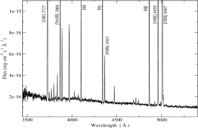
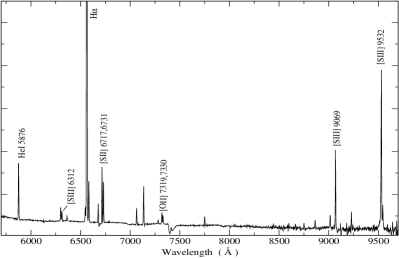
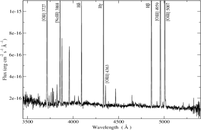
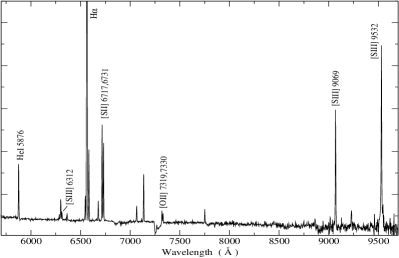
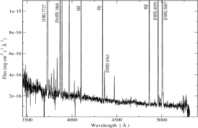
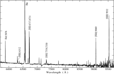
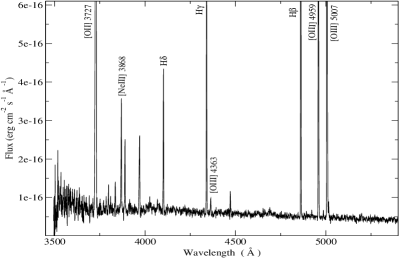
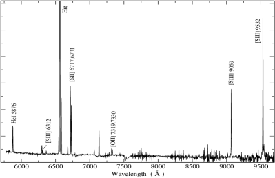
Figure 1: Blue and red CAHA spectra of SDSS J1455, SDSS J1509, SDSS J1528 and SDSS J1540 in the rest frame. The flux scales are the same in both spectral ranges.

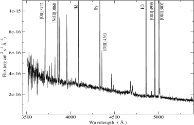
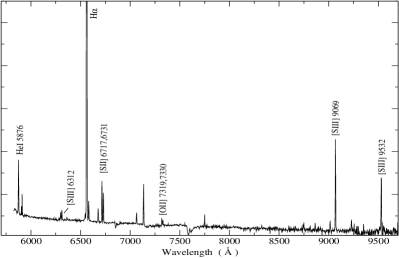
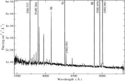
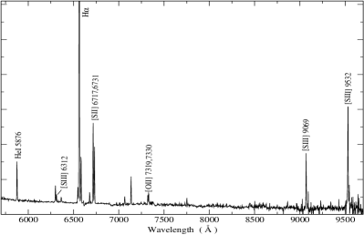
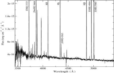
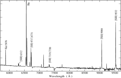
Figure 1: (cont) Blue and red CAHA spectra of SDSS J1616, SDSS J1657 and SDSS J1729. in the rest frame. The flux scales are the same in both spectral ranges.

Table 4: Signal-to-noise ratio attained for each final spectrum.

Object ID	5100-5200	6000-6100	[Sii] $\lambda$ 4068	[Oiii] $\lambda$ 4363	[Nii] $\lambda$ 5755	[Siii] $\lambda$ 6312	[Oii] $\lambda$ 7319	[Oii] $\lambda$ 7330
SDSS J1455	20	50	27	180	—	157	160	126
SDSS J1509	15	40	25	40	—	95	99	82
SDSS J1528	10	33	18	60	—	125	91	73
SDSS J1540	10	35	15	24	—	92	78	62
SDSS J1616	15	40	12	87	—	61	82	53
SDSS J1657	15	35	21	64	—	107	67	47
SDSS J1729	15	35	12	77	29	105	147	122

2.3 Data reduction

Several bias and sky flat field frames were taken at the beginning and end of each night. In addition, two lamp flat fields and one calibration lamp exposure were performed at each telescope position. The calibration lamp used was HeAr. The images were processed and analyzed with IRAF routines in the usual manner. The procedure includes the removal of cosmic rays, bias substraction, division by a normalized flat field and wavelength calibration.

Finally, the spectra were corrected for atmospheric extinction and flux calibrated. Four standard star observations were performed each night, allowing a good spectrophotometric calibration with an estimated accuracy of about 3%, estimated from the differences between the different standard star flux calibration curves.

3 Results

The spectra of the observed Hii galaxies with some of the relevant identified emission lines are shown in Fig. 1. The spectrum of each observed galaxy is split into two panels, with the blue part on the left and the red part on the right.

The emission line fluxes were measured using the SPLOT task in IRAF following the procedure described in Hägele et al. (2006; hereafter Paper I). Following Pérez-Montero & Díaz (2003), the statistical errors associated with the observed emission fluxes have been calculated using the expression

$$\sigma_{l}\,=\,\sigma_{c}N^{1/2}[1+EW/(N\Delta)]^{1/2}$$

where $\sigma_{l}$ is the error in the observed line flux, $\sigma_{c}$ represents the standard deviation in a box near the measured emission line and stands for the error in the continuum placement, N is the number of pixels used in the measurement of the line flux, EW is the line equivalent width, and $\Delta$ is the wavelength dispersion in Å per pixel (González-Delgado et al., 1994). There are several emission lines affected by cosmetic faults or charge transfer in the CCD, internal reflections in the spectrograph, telluric emission lines or atmospheric absorption lines. These lines were excluded from any subsequent analysis. In the case of SDSS J1528, the [Ariii] $\lambda$ 7136 is affected by a sky absorption band. Its observed flux has been scaled to that of the [Ariii] 7751Å line according to the theoretical relation, [Ariii] 7136/[Ariii] 7751 = 4.17, derived from the IONIC task in the STSDAS package of IRAF for a wide temperature range, from 5000 to 50000 K. For SDSS J1616 the [Siii] $\lambda$ 9532 line is affected by strong narrow water-vapour lines and therefore its value has been set to its theoretical ratio to the weaker [Siii] $\lambda$ 9069 Å line, taken to be 2.44.

An underlying stellar population is easily appreciable by the presence of absorption features that depress the Balmer and Paschen emission lines. A pseudo-continuum has been defined at the base of the hydrogen emission lines to measure the line intensities and minimise the errors introduced by the underlying population (see Paper I). We can clearly see the wings of the absorption lines implying that, even though we have used a pseudo-continuum, there is still an absorbed fraction of the emitted flux that we are not able to measure with an acceptable accuracy (see discussion in Díaz, 1988). This fraction is not the same for all lines, nor are the ratios between the absorbed fractions and the emission. In Paper I we estimated that the differences between the measurements obtained using the defined the pseudo-continuum and those made using a multi-Gaussian fit to the absorption and emission components, when this fitting is possible, are, for all the Balmer lines, within the observational errors. This is also expected to be the case for the objects presented here given our selection criterion of large H$\alpha$ equivalent width. At any rate, for the Balmer and Paschen emission lines we have doubled the derived error, $\sigma_{l}$, as a conservative approach to include the uncertainties introduced by the presence of the underlying stellar population.

The absorption features of the underlying stellar population will also affect the helium emission lines to some extent. However, the wings of these absorption lines are narrower than those of hydrogen (see, for example, González-Delgado et al., 2005). Therefore it is difficult to set adequate pseudo-continua at both sides of the lines to measure their fluxes.

The reddening coefficient [$c$(H$\beta$)] has been calculated assuming the galactic extinction law of Miller & Mathews (1972) with $R_{v}$=3.2 and obtained by performing a least square fit to the difference between the theoretical and observed Balmer and Paschen decrements vs. the reddening law whose slope is the logarithmic reddening at the H$\beta$ wavelength:

$$log\Big{(}\frac{I(\lambda)}{I(H\beta)}\Big{)}\,=\,log\Big{(}\frac{F(\lambda)}{F(H\beta)}\Big{)}+c(H\beta)\,f(\lambda)$$

The theoretical Balmer line intensities have been computed using Storey & Hummer (1995) with an iterative method to estimate $t_{e}$ and $N_{e}$ in each case. As $N_{e}$ introduces only a second order effect, for simplicity we assume $N_{e}$ equal to N([Sii]). Due to the large error introduced by the presence of the underlying stellar population, only the four strongest Balmer emission lines (H$\alpha$, H$\beta$, H$\gamma$ and H$\delta$) have been used.

Table LABEL:ratiostot_1 gives the equivalent widths and the reddening corrected emission lines for each observed galaxy together with the reddening constant and its error taken as the uncertainties of the least square fit and the reddening corrected H$\beta$ intensity. The adopted reddening curve, $f(\lambda)$, normalized to H$\beta$, is given in column 2 of the table. The errors in the emission lines were obtained by propagating in quadrature the observational errors in the emission line fluxes and the reddening constant uncertainties.

The relative errors in the emission lines vary from a few percent for the more intense nebular emission lines (e.g. [Oiii] $\lambda\lambda$ 4959,5007, [Sii] $\lambda\lambda$ 6717,6731 or the strongest Balmer emission lines) to 10-35 % for the weakest lines that have less contrast with the continuum noise (e.g. Hei $\lambda\lambda$ 3820,7281, [Ariv] $\lambda$ 4740 or Oi $\lambda$ 8446). For the auroral lines, the fractional errors are between $\sim$3 and $\sim$10 %.

Table 5: Relative reddening corrected line intensities [$F(H\beta)$=$I(H\beta)$=10000]

		SDSS J1455			SDSS J1509				SDSS J1528
$\lambda$ (Å)	f($\lambda$)	-EW	$I(\lambda)$	$I(\lambda)^{\dagger}$	-EW	$I(\lambda)$	$I(\lambda)^{\dagger}$	$I(\lambda)^{\ddagger}$	-EW	$I(\lambda)$	$I(\lambda)^{\ddagger}$
		(Å)			(Å)				(Å)
3727 [Oii]b	0.271	91.6	11154$\pm$164	10920$\pm$400	131.7	15318$\pm$182	20970$\pm$760	18620$\pm$1800	177.4	22882$\pm$294	22390$\pm$2160
3734 H13	0.270	1.1	130$\pm$31	—	3.5	278$\pm$56	—	—	2.8	295$\pm$56	—
3750 H12	0.266	1.8	204$\pm$48	270$\pm$70	2.1	203$\pm$48	300$\pm$80	—	2.9	315$\pm$64	—
3770 H11	0.261	1.9	222$\pm$27	470$\pm$70	2.4	236$\pm$38	460$\pm$80	—	5.0	510$\pm$53	—
3798 H10	0.254	3.7	407$\pm$39	520$\pm$80	4.7	410$\pm$60	480$\pm$90	—	7.6	709$\pm$70	—
3820 Hei	0.249	0.6	81$\pm$16	—	0.6	66$\pm$15	—	—	—	—	—
3835 H9	0.246	5.0	574$\pm$68	750$\pm$70	6.3	537$\pm$59	710$\pm$90	—	7.6	820$\pm$58	—
3868 [Neiii]	0.238	37.1	4792$\pm$105	5230$\pm$200	32.5	3501$\pm$109	4120$\pm$180	3980$\pm$380	39.0	4717$\pm$180	5370$\pm$520
3889 Hei+H8	0.233	16.1	1816$\pm$99	—	16.4	1622$\pm$81	—	—	21.1	2151$\pm$74	—
3968 [Neiii]+H7	0.216	27.6	2996$\pm$71	—	20.6	2262$\pm$113	—	2570$\pm$250	35.3	3231$\pm$143	3020$\pm$290
4026 [Nii]+Hei	0.203	1.2	148$\pm$22	—	1.4	157$\pm$19	—	—	1.9	208$\pm$55	—
4068 [Sii]	0.195	1.2	158$\pm$11	—	1.7	199$\pm$19	—	—	2.0	214$\pm$18	—
4102 H$\delta$	0.188	24.4	2580$\pm$57	2590$\pm$120	26.8	2420$\pm$61	2730$\pm$140	2820$\pm$270	41.6	2824$\pm$94	2820$\pm$270
4340 H$\gamma$	0.142	48.8	4562$\pm$70	4710$\pm$180	54.1	4395$\pm$76	4860$\pm$200	4680$\pm$450	62.4	4773$\pm$76	4790$\pm$460
4363 [Oiii]	0.138	9.8	1022$\pm$35	990$\pm$60	4.2	420$\pm$21	500$\pm$60	550$\pm$80	5.4	500$\pm$22	—
4471 Hei	0.106	4.1	380$\pm$23	—	5.1	454$\pm$32	—	—	5.8	465$\pm$28	—
4658 [Feiii]	0.053	0.3	28$\pm$4	110$\pm$40	1.1	106$\pm$12	110$\pm$50	—	1.6	125$\pm$17	—
4686 Heii	0.045	0.8	75$\pm$9	—	—	—	—	—	—	—	—
4713 [Ariv]+Hei	0.038	2.7	223$\pm$17	—	—	—	—	—	1.0	79$\pm$24	—
4740 [Ariv]	0.031	1.2	103$\pm$14	110$\pm$40	—	—	—	—	—	—	—
4861 H$\beta$	0.000	132.8	10000$\pm$67	10000$\pm$340	123.4	10000$\pm$74	10000$\pm$350	10000$\pm$960	171.4	10000$\pm$116	10000$\pm$960
4881 [Feiii]	-0.005	0.3	25$\pm$6	—	—	—	—	—	—	—	—
4921 Hei	-0.014	1.3	96$\pm$11	—	1.1	99$\pm$12	—	—	1.9	114$\pm$17	—
4959 [Oiii]	-0.024	254.3	20456$\pm$134	21040$\pm$680	190.7	16751$\pm$148	16610$\pm$560	16600$\pm$1600	256.2	16557$\pm$173	15850$\pm$1530
4986 [Feiii]c	-0.030	0.9	71$\pm$18	90$\pm$40	1.3	114$\pm$16	140$\pm$40	—	2.0	129$\pm$31	—
5007 [Oiii]	-0.035	782.2	61355$\pm$336	—	571.3	49942$\pm$153	—	50120$\pm$4840	764.2	48932$\pm$292	47860$\pm$4620
5015 Hei	-0.037	3.1	234$\pm$20	—	2.9	249$\pm$26	—	—	5.4	324$\pm$32	—
5199 [Ni]	-0.078	0.7	48$\pm$10	—	1.4	105$\pm$20	—	—	—	—	—
5270 [Feiii]a	-0.094	0.4	26$\pm$5	—	—	—	—	—	—	—	—
5755 [Nii]	-0.188	—	—	—	—	—	—	—	—	—	—
5876 Hei	-0.209	22.4	1140$\pm$35	1090$\pm$60	21.6	1268$\pm$59	1120$\pm$70	1230$\pm$120	28.5	1227$\pm$36	—
6300 [Oi]	-0.276	5.5	257$\pm$11	210$\pm$30	7.7	452$\pm$26	400$\pm$40	—	11.3	438$\pm$18	1200$\pm$180
6312 [Siii]	-0.278	3.6	160$\pm$6	150$\pm$30	2.8	164$\pm$9	160$\pm$40	—	4.3	168$\pm$10	—
6364 [Oi]	-0.285	2.0	95$\pm$19	—	2.6	146$\pm$19	—	—	3.8	145$\pm$12	—
6548 [Nii]	-0.311	6.2	273$\pm$15	—	9.6	541$\pm$28	—	—	19.4	721$\pm$45	—
6563 H$\alpha$	-0.313	646.8	27756$\pm$183	28190$\pm$980	522.6	27969$\pm$141	28570$\pm$1020	28180$\pm$2720	823.2	28888$\pm$169	29510$\pm$2850
6584 [Nii]	-0.316	18.2	792$\pm$19	750$\pm$50	25.4	1387$\pm$37	1370$\pm$70	1910$\pm$180	54.0	1959$\pm$43	1450$\pm$140
6678 Hei	-0.329	9.7	350$\pm$38	—	7.2	392$\pm$15	—	—	10.3	350$\pm$10	—
6717 [Sii]	-0.334	21.9	1000$\pm$26	1720$\pm$70ℷ	35.8	1966$\pm$48	2880$\pm$110ℷ	2140$\pm$210	57.1	1923$\pm$75	1320$\pm$200
6731 [Sii]	-0.336	14.5	788$\pm$22	—	27.1	1488$\pm$40	—	1780$\pm$170	43.7	1422$\pm$58	1120$\pm$170
7065 Hei	-0.377	8.3	293$\pm$12	—	6.0	302$\pm$19	—	—	9.6	297$\pm$17	—
7136 [Ariii]	-0.385	18.5	662$\pm$30	590$\pm$40	19.1	982$\pm$29	790$\pm$50	1200$\pm$120	19.1	—	—
7281 Heia	-0.402	2.1	78$\pm$9	—	—	—	—	—	2.0	60$\pm$5	—
7319 [Oii]d	-0.406	5.3	181$\pm$9	290$\pm$40ℶ	4.8	203$\pm$9	410$\pm$50ℶ	—	10.0	296$\pm$17	—
7330 [Oii]e	-0.407	4.1	142$\pm$8	—	4.0	167$\pm$8	—	—	8.2	238$\pm$12	—
7751 [Ariii]	-0.451	4.7	154$\pm$9	—	5.2	242$\pm$16	—	—	8.1	210$\pm$13	—
8446 Oi	-0.513	1.7	46$\pm$8	—	1.6	68$\pm$10	—	—	—	—	—
8503 P16	-0.518	2.6	59$\pm$10	—	—	—	—	—	—	—	—
8546 P15	-0.521	—	—	—	—	—	—	—	—	—	—
8599 P14	-0.525	—	—	—	3.5	100$\pm$33	—	—	4.8	72$\pm$13	—
8665 P13	-0.531	4.9	105$\pm$18	—	4.0	118$\pm$42	—	—	5.7	102$\pm$15	—
8751 P12	-0.537	7.9	147$\pm$17	—	5.0	154$\pm$47	—	—	12.0	145$\pm$16	—
8865 P11	-0.546	8.3	181$\pm$22	—	11.4	297$\pm$65	—	—	24.5	199$\pm$43	—
9014 P10	-0.557	11.4	269$\pm$32	—	33.6	447$\pm$93	—	—	—	—	—
9069 [Siii]	-0.561	50.8	1154$\pm$59	—	82.1	2546$\pm$120	—	—	88.1	1688$\pm$127	—
9229 P9	-0.572	33.0	400$\pm$50	—	27.2	595$\pm$98	—	—	31.9	292$\pm$86	—
9532 [Siii]	-0.592	140.1	3278$\pm$148	—	176.3	5181$\pm$256	—	—	506.6	4049$\pm$289	—
9547 P8	-0.593	21.7	455$\pm$69	—	43.5	876$\pm$129	—	—	—	—	—
I(H$\beta$)(erg seg-1 cm-2)		1.49 $\times$ 10-14			1.35 $\times$ 10-14				1.73 $\times$ 10-14
c(H$\beta$)		0.13$\pm$0.01		0.05	0.07$\pm$0.01		0.08	0.05	0.04$\pm$0.01		0.15
a possibly blend with an unknown line; b [Oii] $\lambda\lambda$ 3726 + 3729; c [Feiii] $\lambda\lambda$ 4986 + 4987; d [Oii] $\lambda\lambda$ 7318 + 7320; e [Oii] $\lambda\lambda$ 7330 + 7331. † from Izotov et al. (2006); they gave ℷ [Sii] $\lambda\lambda$ 6717 + 6731 and ℶ [Oii] $\lambda\lambda$ 7319 + 7330. ‡ from Peimbert & Torres-Peimbert (1992).

Table 5: (cont.) Relative reddening corrected line intensities [$F(H\beta)$=$I(H\beta)$=10000]

		SDSS J1540				SDSS J1616			SDSS J1657
$\lambda$ (Å)	f($\lambda$)	-EW	$I(\lambda)$	$I(\lambda)^{\dagger}$	$I(\lambda)^{\S}$	-EW	$I(\lambda)$	$I(\lambda)^{\dagger}$	-EW	$I(\lambda)$
		(Å)				(Å)			(Å)
3727 [Oii]b	0.271	232.8	21793$\pm$256	—	—	33.5	8491$\pm$196	—	120.1	18832$\pm$230
3734 H13	0.270	2.6	272$\pm$48	—	—	—	—	—	—	—
3750 H12	0.266	—	—	—	—	1.8	377$\pm$101	—	1.9	232$\pm$47
3770 H11	0.261	2.7	314$\pm$61	—	—	1.5	357$\pm$113	—	2.3	293$\pm$40
3798 H10	0.254	4.8	581$\pm$93	760$\pm$90	810$\pm$280	2.1	447$\pm$92	—	4.1	500$\pm$68
3820 Hei	0.249	1.5	166$\pm$23	—	—	—	—	—	—	—
3835 H9	0.246	6.2	678$\pm$85	920$\pm$90	940$\pm$260	3.1	638$\pm$90	790$\pm$110	7.1	780$\pm$93
3868 [Neiii]	0.238	15.2	2142$\pm$82	1860$\pm$90	—	17.2	4105$\pm$166	5450$\pm$230	23.1	3262$\pm$132
3889 Hei+H8	0.233	11.6	1445$\pm$113	—	—	7.3	1591$\pm$112	—	14.0	1826$\pm$95
3968 [Neiii]+H7	0.216	21.9	2309$\pm$144	—	—	11.7	2563$\pm$125	—	22.4	2456$\pm$121
4026 [Nii]+Hei	0.203	20.6	2505$\pm$78	—	—	0.4	94$\pm$15	—	1.1	155$\pm$16
4068 [Sii]	0.195	1.7	231$\pm$18	—	—	0.5	108$\pm$10	—	1.4	198$\pm$15
4102 H$\delta$	0.188	23.7	2589$\pm$63	2570$\pm$120	2590$\pm$130	13.3	2530$\pm$67	2800$\pm$150	20.9	2432$\pm$65
4340 H$\gamma$	0.142	44.2	4753$\pm$61	4670$\pm$170	4640$\pm$100	26.7	4597$\pm$89	5000$\pm$200	43.1	4417$\pm$97
4363 [Oiii]	0.138	4.5	291$\pm$17	220$\pm$40	220$\pm$50	4.5	851$\pm$26	980$\pm$80	4.5	524$\pm$24
4471 Hei	0.106	4.7	463$\pm$33	—	—	2.5	404$\pm$32	—	4.2	443$\pm$33
4658 [Feiii]	0.053	0.7	78$\pm$14	—	—	—	—	—	1.0	107$\pm$16
4686 Heii	0.045	—	—	—	—	2.1	329$\pm$43	310$\pm$60	1.2	126$\pm$14
4713 [Ariv]+Hei	0.038	—	—	—	—	—	—	—	—	—
4740 [Ariv]	0.031	—	—	—	—	0.5	69$\pm$22	—	—	—
4861 H$\beta$	0.000	122.4	10000$\pm$76	10000$\pm$340	10000$\pm$100	83.0	10000$\pm$96	10000$\pm$350	117.8	10000$\pm$79
4881 [Feiii]	-0.005	—	—	—	—	—	—	—	—	—
4921 Hei	-0.014	1.2	109$\pm$15	—	—	0.9	116$\pm$13	—	0.8	75$\pm$14
4959 [Oiii]	-0.024	114.4	10480$\pm$75	9920$\pm$340	9830$\pm$90	156.5	20492$\pm$147	20380$\pm$680	152.5	14333$\pm$127
4986 [Feiii]c	-0.030	0.9	84$\pm$12	180$\pm$40	—	—	—	—	1.4	135$\pm$28
5007 [Oiii]	-0.035	348.3	30942$\pm$188	—	29000$\pm$230	480.7	61516$\pm$371	—	455.1	43082$\pm$240
5015 Hei	-0.037	2.7	235$\pm$16	—	—	1.8	225$\pm$26	—	2.4	222$\pm$23
5199 [Ni]	-0.078	2.0	151$\pm$27	—	—	—	—	—	2.0	157$\pm$26
5270 [Feiii]a	-0.094	—	—	—	—	—	—	—	—	—
5755 [Nii]	-0.188	—	—	—	—	—	—	—	—	—
5876 Hei	-0.209	19.2	1155$\pm$36	1090$\pm$60	—	13.7	1063$\pm$75	970$\pm$60	18.9	1116$\pm$44
6300 [Oi]	-0.276	6.4	335$\pm$14	330$\pm$30	—	1.7	104$\pm$18	170$\pm$40	8.1	438$\pm$16
6312 [Siii]	-0.278	2.6	139$\pm$10	110$\pm$30	—	3.2	186$\pm$11	200$\pm$40	3.7	201$\pm$9
6364 [Oi]	-0.285	2.3	122$\pm$17	—	—	0.9	51$\pm$13	—	2.8	152$\pm$18
6548 [Nii]	-0.311	13.9	735$\pm$34	—	—	2.8	160$\pm$13	—	9.4	464$\pm$23
6563 H$\alpha$	-0.313	581.9	28626$\pm$162	28770$\pm$1010	28730$\pm$220	517.2	27892$\pm$145	28160$\pm$1000	571.3	27772$\pm$153
6584 [Nii]	-0.316	42.2	2116$\pm$66	1960$\pm$90	—	8.0	434$\pm$23	380$\pm$40	28.8	1428$\pm$47
6678 Hei	-0.329	6.8	316$\pm$15	—	—	5.9	296$\pm$18	—	6.7	315$\pm$18
6717 [Sii]	-0.334	52.6	2609$\pm$52	4330$\pm$130ℷ	2450$\pm$30	15.3	774$\pm$23	1400$\pm$70ℷ	47.4	2207$\pm$57
6731 [Sii]	-0.336	41.7	1919$\pm$50	—	1800$\pm$30	11.9	581$\pm$22	—	32.2	1598$\pm$43
7065 Hei	-0.377	4.5	200$\pm$9	—	—	5.1	229$\pm$14	—	5.6	235$\pm$10
7136 [Ariii]	-0.385	23.2	892$\pm$52	880$\pm$50	—	17.4	736$\pm$44	690$\pm$50	16.4	717$\pm$26
7281 Heia	-0.402	3.1	115$\pm$10	—	—	—	—	—	0.9	41$\pm$7
7319 [Oii]d	-0.406	6.3	273$\pm$16	500$\pm$40ℶ	460$\pm$40ϰ	3.4	138$\pm$11	260$\pm$40ℶ	12.3	302$\pm$17
7330 [Oii]e	-0.407	5.0	216$\pm$12	—	—	2.2	90$\pm$7	—	8.8	211$\pm$14
7751 [Ariii]	-0.451	6.1	223$\pm$26	—	—	4.5	166$\pm$21	—	4.6	177$\pm$22
8446 Oi	-0.513	—	—	—	—	—	—	—	—	—
8503 P16	-0.518	—	—	—	—	2.6	60$\pm$20	—	—	—
8546 P15	-0.521	—	—	—	—	1.6	38$\pm$14	—	—	—
8599 P14	-0.525	—	—	—	—	5.6	109$\pm$20	—	—	—
8665 P13	-0.531	—	—	—	—	8.0	153$\pm$31	—	7.7	144$\pm$53
8751 P12	-0.537	—	—	—	—	8.1	181$\pm$32	—	4.2	101$\pm$29
8865 P11	-0.546	—	—	—	—	9.6	182$\pm$34	—	8.5	211$\pm$34
9014 P10	-0.557	12.9	237$\pm$68	—	—	24.4	319$\pm$44	—	15.4	167$\pm$36
9069 [Siii]	-0.561	67.2	2095$\pm$62	2020$\pm$100	—	74.3	1647$\pm$62	1470$\pm$80	59.2	1400$\pm$99
9229 P9	-0.572	—	—	—	—	14.2	272$\pm$51	—	16.9	263$\pm$47
9532 [Siii]	-0.592	236.8	5331$\pm$331	—	—	74.3	4011$\pm$153	—	157.3	3674$\pm$257
9547 P8	-0.593	29.0	573$\pm$145	—	—	—	—	—	—	—
I(H$\beta$)(erg seg-1 cm-2)		0.53 $\times$ 10-14				1.36 $\times$ 10-14			0.63 $\times$ 10-14
c(H$\beta$)		0.22$\pm$0.01		0.07	0.07	0.02$\pm$0.01		0.06	0.05$\pm$0.01
a possibly blend with an unknown line; b [Oii] $\lambda\lambda$ 3726 + 3729; c [Feiii] $\lambda\lambda$ 4986 + 4987; d [Oii] $\lambda\lambda$ 7318 + 7320; e [Oii] $\lambda\lambda$ 7330 + 7331. † from Izotov et al. (2006); they gave ℷ [Sii] $\lambda\lambda$ 6717 + 6731 and ℶ [Oii] $\lambda\lambda$ 7319 + 7330. § from Kniazev et al. (2004); they gave ϰ [Oii] $\lambda\lambda$ 7319 + 7330.

Table 5: (cont.) Relative reddening corrected line intensities [$F(H\beta)$=$I(H\beta)$=10000]

		SDSS J1729
$\lambda$ (Å)	f($\lambda$)	-EW	$I(\lambda)$	$I(\lambda)^{\dagger}$	$I(\lambda)^{\S}$
		(Å)
3727 [Oii]b	0.271	135.8	17622$\pm$243	—	—
3734 H13	0.270	1.4	175$\pm$54	—	—
3750 H12	0.266	4.2	397$\pm$89	370$\pm$70	—
3770 H11	0.261	7.6	713$\pm$88	480$\pm$70	—
3798 H10	0.254	5.2	598$\pm$71	620$\pm$60	370$\pm$200
3820 Hei	0.249	—	—	—	—
3835 H9	0.246	7.6	721$\pm$64	900$\pm$60	640$\pm$140
3868 [Neiii]	0.238	34.9	4787$\pm$172	3730$\pm$140	—
3889 Hei+H8	0.233	16.9	2058$\pm$83	—	—
3968 [Neiii]+H7	0.216	24.7	2969$\pm$129	—	—
4026 [Nii]+Hei	0.203	2.4	311$\pm$30	—	—
4068 [Sii]	0.195	0.9	122$\pm$11	—	—
4102 H$\delta$	0.188	24.9	2765$\pm$63	2540$\pm$100	2430$\pm$100
4340 H$\gamma$	0.142	48.7	4839$\pm$84	4760$\pm$170	4750$\pm$80
4363 [Oiii]	0.138	5.9	660$\pm$30	510$\pm$40	510$\pm$40
4471 Hei	0.106	5.2	516$\pm$24	—	—
4658 [Feiii]	0.053	0.8	90$\pm$14	—	—
4686 Heii	0.045	—	—	—	—
4713 [Ariv]+Hei	0.038	0.7	77$\pm$16	—	—
4740 [Ariv]	0.031	0.4	40$\pm$10	—	—
4861 H$\beta$	0.000	125.6	10000$\pm$83	10000$\pm$320	10000$\pm$80
4881 [Feiii]	-0.005	—	—	—	—
4921 Hei	-0.014	1.4	122$\pm$12	—	—
4959 [Oiii]	-0.024	185.8	17097$\pm$146	16990$\pm$540	17470$\pm$90
4986 [Feiii]c	-0.030	0.6	56$\pm$18	80$\pm$30	—
5007 [Oiii]	-0.035	555.4	51541$\pm$418	—	52320$\pm$300
5015 Hei	-0.037	1.9	177$\pm$12	—	—
5199 [Ni]	-0.078	—	—	—	—
5270 [Feiii]a	-0.094	0.7	55$\pm$12	—	—
5755 [Nii]	-0.188	0.8	60$\pm$6	—	—
5876 Hei	-0.209	17.4	1261$\pm$37	1130$\pm$50	—
6300 [Oi]	-0.276	4.0	253$\pm$16	260$\pm$30	—
6312 [Siii]	-0.278	2.7	176$\pm$11	170$\pm$30	—
6364 [Oi]	-0.285	1.2	78$\pm$11	—	—
6548 [Nii]	-0.311	12.5	771$\pm$21	—	—
6563 H$\alpha$	-0.313	476.9	28700$\pm$163	28510$\pm$960	28530$\pm$150
6584 [Nii]	-0.316	35.8	2189$\pm$52	2080$\pm$80	—
6678 Hei	-0.329	6.0	355$\pm$12	—	—
6717 [Sii]	-0.334	21.7	1286$\pm$32	2160$\pm$80ℷ	1220$\pm$20
6731 [Sii]	-0.336	17.3	1009$\pm$30	—	950$\pm$20
7065 Hei	-0.377	5.7	265$\pm$18	—	—
7136 [Ariii]	-0.385	18.0	864$\pm$41	950$\pm$50	—
7281 Heia	-0.402	1.5	75$\pm$11	—	—
7319 [Oii]d	-0.406	4.6	233$\pm$8	430$\pm$40ℶ	390$\pm$20ϰ
7330 [Oii]e	-0.407	3.9	194$\pm$9	—	—
7751 [Ariii]	-0.451	4.5	210$\pm$10	—	—
8446 Oi	-0.513	—	—	—	—
8503 P16	-0.518	3.0	102$\pm$32	—	—
8546 P15	-0.521	—	—	—	—
8599 P14	-0.525	2.9	96$\pm$17	—	—
8665 P13	-0.531	4.7	140$\pm$20	—	—
8751 P12	-0.537	7.0	205$\pm$35	—	—
8865 P11	-0.546	—	—	—	—
9014 P10	-0.557	8.1	236$\pm$54	—	—
9069 [Siii]	-0.561	58.5	2092$\pm$95	—	—
9229 P9	-0.572	19.9	400$\pm$64	—	—
9532 [Siii]	-0.592	181.5	4718$\pm$250	—	—
9547 P8	-0.593	20.3	480$\pm$69	—	—
I(H$\beta$)(erg seg-1 cm-2)		2.40 $\times$ 10-14
c(H$\beta$)		0.03$\pm$0.01		0.02	0.04
a possibly blend with an unknown line; b [Oii] $\lambda\lambda$ 3726 + 3729; c [Feiii] $\lambda\lambda$ 4986 + 4987; d [Oii] $\lambda\lambda$ 7318 + 7320; e [Oii] $\lambda\lambda$ 7330 + 7331. † from Izotov et al. (2006); they gave ℷ [Sii] $\lambda\lambda$ 6717 + 6731 and ℶ [Oii] $\lambda\lambda$ 7319 + 7330. § from Kniazev et al. (2004); they gave ϰ [Oii] $\lambda\lambda$ 7319 + 7330.

4 Electron densities and temperatures from forbidden lines

The physical conditions of the ionised gas, including electron temperatures and electron density, have been derived using the five-level statistical equilibrium atom approximation in the task TEMDEN of the STSDAS package of the software IRAF (de Robertis, Dufour & Hunt, 1987; Shaw & Dufour, 1995). The atomic coefficients used with their corresponding references are given in table 6.

The electron density, $N_{e}$, has been derived from the [Sii] $\lambda\lambda$ 6717 / 6731 Å line ratio. In all the observed galaxies the electron densities have been found to be lower than 200 cm^-3, well below the critical density for collisional deexcitation. We were not able to estimate the density from line ratios such as [Ariv] $\lambda\lambda$ 4713,4740 Å, representative of the higher ionisation zones, hence we are not able to determine any existing distribution in density.

Table 6: Sources of the effective collision strengths of each ion.

Ion	references
Oii	Pradhan (1976)
Oiii, Nii	Lennon & Burke (1994)
Sii	Ramsbottom, Bell & Stafford (1996)
Siii	Tayal & Gupta (1999)
Neiii	Butler & Zeippen (1994)
Ariii	Galavis, Mendoza & Zeippen (1995)
Ariv	Zeippen, Le Bourlot & Butler (1987)

Table 7: Emission-line ratios used to derive electron densities and temperatures.

	ratios
Ne([Sii])	RS2 = I(6717) / I(6731)
te([Oiii])	RO3 = (I(4959)+I(5007)) / I(4363)
te([Oii])	RO2 = I(3727) / (I(7319)+I(7330))
te([Siii])	RS3 = (I(9069)+I(9532)) / I(6312)
te([Sii])	R${}_{S2}^{\prime}$ = (I(6717)+I(6731)) / (I(4068)+I(4074))
te([Nii])	RN2 = (I(6548)+I(6584)) / I(5755)

For all the objects we have derived the electron temperatures of [Oii], [Oiii], [Sii] and [Siii]. Only for one object, SDSS J1729, it was possible to derive T_e([Nii]). The emission-line ratios used to calculate each temperature are summarized in table 7. Adequate fitting functions have been derived from the TEMDEM task and are given below:

$$t_{e}([O{\textrm{\sc iii}}])\,=\,0.8254\,-\,0.0002415\,R_{O3}\,+\,\frac{47.77}{R_{O3}}$$

$$t_{e}([S{\textrm{\sc iii}}])\,=\,\frac{R_{S3}\,+\,36.4}{1.8\,R_{S3}\,-3.01}$$

$$t_{e}([O{\textrm{\sc ii}}])\,=\,0.23+0.0017\,R_{O2}\,+\,\frac{38.3}{R_{O2}}\,+\,f_{1}(n_{e})$$

$$t_{e}([S{\textrm{\sc ii}}]\,=\,1.92\,-\,0.0375\,R_{S2}^{\prime}\,-\,\frac{14.5}{R_{S2}^{\prime}}\,+\,\frac{105.64}{R_{S2}^{\prime 2}}\,+\,f_{2}(n_{e})$$

$$t_{e}([N{\textrm{\sc ii}}])\,=\,0.537\,+0.000253\,R_{N2}\,+\,\frac{42.13}{R_{N2}}$$

where $n_{e}$ = 10${}^{-4}\,N_{e}$ and $f_{1}(n_{e})$,$f_{2}(n_{e})$ $<<$ 1 for $N_{e}$ $<$ 1000 cm^-3. The above expressions are valid in the temperature range between 7000 and 23000 K and the errors involved in the fittings are always lower than observational errors by factors between 5 and 10.

In order to calculate the errors associated with the derived electron temperatures and densities, we have propagated the emission line intensity errors listed in Table LABEL:ratiostot_1 through our calculations.

Both the [Oii] $\lambda\lambda$ 7319,7330 Å and the [Nii] $\lambda$ 5755 Å  lines have a contribution by direct recombination which increases with temperature. Such emission, however, can be quantified and corrected for as:

$$\frac{I_{R}(7319+7330)}{I(H\beta)}\,=\,9.36\,t^{0.44}\,\frac{O^{2+}}{H^{+}}$$

$$\frac{I_{R}(5755)}{I(H\beta)}\,=\,3.19\,t^{0.30}\,\frac{N^{2+}}{H^{+}}$$

where $t$ denotes the electron temperature in units of 10⁴ K (Liu et al., 2000). Using the calculated [Oiii] electron temperatures, we have estimated these contributions to be less than 4% in all cases and therefore we have not corrected for this effect, but we have including it as an additional source of error. In the worst cases this amounts to about 10 % of the total error. The expressions above, however, are only valid in the range of temperatures between 5000 and 10000 K in the case of [Oii] and between 5000 and 20000 K in the case of [Nii]. While the [Oiii] temperatures found in our objects are inside the range of validity for [Nii], they are slightly over that range for [Oii]. At any rate, the relative contribution of recombination to collisional intensities decreases rapidly with increasing temperature.

Table 8: Electron densities and temperatures for the observed galaxies.

	n([Sii])	te([Oiii])	te([Oii])	te([Siii])	te([Sii])	te([Nii])
SDSS J1455	94 $\pm$ 40	1.40 $\pm$ 0.02	1.33 $\pm$ 0.07	1.37 $\pm$ 0.05	1.31 $\pm$ 0.11	—
SDSS J1509	85 $\pm$ 45	1.09 $\pm$ 0.01	1.18 $\pm$ 0.05	1.02 $\pm$ 0.04	0.89 $\pm$ 0.07	—
SDSS J1528	60:	1.16 $\pm$ 0.01	1.17 $\pm$ 0.05	1.21 $\pm$ 0.06	0.99 $\pm$ 0.07	—
SDSS J1540	47 $\pm$ 38	1.13 $\pm$ 0.02	1.15 $\pm$ 0.06	0.97 $\pm$ 0.04	0.85 $\pm$ 0.05	—
SDSS J1616	54:	1.30 $\pm$ 0.01	1.29 $\pm$ 0.09	1.29 $\pm$ 0.06	1.21 $\pm$ 0.12	—
SDSS J1657	30:	1.23 $\pm$ 0.02	1.33 $\pm$ 0.07	1.45 $\pm$ 0.08	0.88 $\pm$ 0.05	—
SDSS J1729	109 $\pm$ 47	1.26 $\pm$ 0.02	1.16 $\pm$ 0.04	1.13 $\pm$ 0.05	0.82 $\pm$ 0.06	1.40 $\pm$ 0.09
densities in $cm^{-3}$ and temperatures in 104 K

The derived electron densities and temperatures for the seven observed objects are given in Table 8 along with their corresponding errors.

5 Chemical abundances

We have derived the ionic chemical abundances of the different species using the strongest available emission lines detected in the analysed spectra and the task IONIC of the STSDAS package in IRAF. This package is also based on the five-level statistical equilibrium atom approximation (De Robertis, Dufour & Hunt, 1987; Shaw & Dufour, 1995).

The total abundances have been derived by taking into account, when required, the unseen ionization stages of each element, using the appropriate ICF for each species:

$$\frac{X}{H}=ICF(X^{+i})\cdot\frac{X^{+i}}{H^{+}}$$

5.1 Ionic abundances

5.1.1 Helium

We have used the well detected and measured Hei $\lambda\lambda$ 4471, 5876, 6678 and 7065 Å lines, to calculate the abundances of once ionized helium. For three of the objects also the Heii $\lambda$ 4686 Å line was measured allowing the calculation of twice ionized He. The He lines arise mainly from pure recombination, although they could have some contribution from collisional excitation and be affected by self-absorption (see Olive & Skillman, 2001, 2004, for a complete treatment of these effects). We have taken the electron temperature of [Oiii] as representative of the zone where the He emission arises since at any rate ratios of recombination lines are weakly sensitive to electron temperature. We have used the equations given by Olive & Skillman to derive the He⁺/H⁺ value, using the theoretical emissivities scaled to H$\beta$ from Benjamin et al. (1999) and the expressions for the collisional correction factors from Kingdon & Ferland (1995). We have not made, however, any corrections for fluorescence (three of the used helium lines have a small dependence with optical depth effects but the observed objects have low densities) nor for the presence of an underlying stellar population. To calculate the abundance of twice ionized helium we have used equation (9) from Kunth & Sargent (1983). The results obtained for each line and their corresponding errors are presented in table 5.1.1, along with the adopted value for He⁺/H⁺ that is the average, weighted by the errors, of the different ionic abundances derived from each Hei emission line. This value is dubbed “adopted B99” in the Table.

We have also calculated the average values of He⁺/H⁺ from the HeI lines $\lambda\lambda$4471, 5876, 6678, 7065 Å and the corresponding errors, obtained using Olive and Skillman (2004) minimization technique with our derived values of n_e([SII]) and T_e([OIII]) and Porter et al. (2005) He emissivities. We solved simultaneously for underlying stellar absorptions and optical depth. The values are shown in Table 5.1.1 under P05. We found no significant differences for the objects in this paper in the Helium abundances obtained using the two different sets of He emissivities. On the other hand following this method is crucial when trying to determine He abundances to better than 2 percent (like e.g. for determining a value of the primordial He). We chose to wait for a complete error budget determination from the atomic physics parameters (Porter in preparation, private communication) before adopting the latter values for the He abundances.

Table 9: Ionic and total chemical abundances for helium.

	$\lambda$ (Å)	SDSS J1455	SDSS J1509	SDSS J1528	SDSS J1540	SDSS J1616	SDSS J1657	SDSS J1729
$He^{+}/H^{+}$	4471	0.079$\pm$0.004	0.092$\pm$0.006	0.095$\pm$0.005	0.094$\pm$0.006	0.084$\pm$0.006	0.091$\pm$0.007	0.106$\pm$0.004
	5876	0.089$\pm$0.002	0.094$\pm$0.004	0.093$\pm$0.002	0.087$\pm$0.002	0.082$\pm$0.006	0.086$\pm$0.003	0.096$\pm$0.003
	6678	0.098$\pm$0.010	0.103$\pm$0.004	0.094$\pm$0.002	0.084$\pm$0.004	0.081$\pm$0.005	0.086$\pm$0.005	0.097$\pm$0.003
	7065	0.104$\pm$0.005	0.122$\pm$0.008	0.120$\pm$0.007	0.082$\pm$0.004	0.087$\pm$0.006	0.093$\pm$0.005	0.099$\pm$0.008
	adopted B99	0.090$\pm$0.010	0.100$\pm$0.012	0.095$\pm$0.013	0.086$\pm$0.005	0.083$\pm$0.002	0.088$\pm$0.003	0.098$\pm$0.004
	P05	0.096$\pm$0.014	0.102 $\pm$0.011	0.096$\pm$0.010	0.089$\pm$0.010	0.084$\pm$0.012	0.089$\pm$0.009	0.100$\pm$0.010
$He^{2+}/H^{+}$	4686	0.0007$\pm$0.0001	—	—	—	0.0029$\pm$0.0004	0.0011$\pm$0.0001	—
(He/H)		0.090$\pm$0.010	—	—	—	0.086$\pm$0.002	0.089$\pm$0.003	—

5.1.2 Forbidden lines

We have derived appropriate fittings to the IONIC task results following the functional form given by Pagel et al. (1992). These expressions are listed below:

$$12\,+\,log(O^{+}/H^{+})\,=\,log\frac{I(3727+3729)}{I(H\beta)}\,+\,5.992\,+$$

$$+\,\frac{1.583}{t_{e}}\,-\,0.681\,log\,t_{e}\,+\,log(1+2.3\,n_{e})$$

$$12\,+\,log(O^{2+}/H^{+})\,=\,log\frac{I(4959+5007)}{I(H\beta)}\,+\,6.144\,+$$

$$+\,\frac{1.251}{t_{e}}\,-\,0.550\,log\,t_{e}$$

$$12\,+\,log(S^{+}/H^{+})\,=\,log\frac{I(6717+6731)}{I(H\beta)}\,+\,5.423\,+$$

$$+\,\frac{0.929}{t_{e}}\,-\,0.280\,log\,t_{e}\,+\,log(1+1.0\,n_{e})$$

$$12\,+\,log(S^{2+}/H^{+})\,=\,log\frac{I(9069+9532)}{I(H\beta)}\,+\,5.80\,+$$

$$+\,\frac{0.77}{t_{e}}\,-\,0.22\,log\,t_{e}$$

$$12\,+\,log(N^{+}/H^{+})\,=\,log\frac{I(6548+6584)}{I(H\beta)}\,+\,6.273\,+$$

$$+\,\frac{0.894}{t_{e}}\,-\,0.592\,log\,t_{e}$$

$$log\,(N^{+}/O^{+})\,=\,log\frac{I(6548+6584)}{I(3727+3729)}\,+\,0.281\,-$$

$$-\,\frac{0.689}{t_{e}}\,+\,0.089\,log\,t_{e}$$

$$12\,+\,log(Ne^{2+}/H^{+})\,=\,log\frac{I(3868)}{I(H\beta)}\,+\,6.486\,+$$

$$+\,\frac{1.558}{t_{e}}\,-\,0.504\,log\,t_{e}$$

$$12\,+\,log(Ar^{2+}/H^{+})\,=\,log\frac{I(7137)}{I(H\beta)}\,+\,6.157\,+$$

$$+\,\frac{0.808}{t_{e}}\,-\,0.508\,log\,t_{e}$$

$$12\,+\,log(Ar^{3+}/H^{+})\,=\,log\frac{I(4740)}{I(H\beta)}\,+\,5.705\,+$$

$$+\,\frac{1.246}{t_{e}}\,-\,0.156\,log\,t_{e}$$

$$12\,+\,log(Fe^{2+}/H^{+})\,=\,log\frac{I(4658)}{I(H\beta)}\,+\,3.504\,+$$

$$+\,\frac{1.298}{t_{e}}\,-\,0.483\,log\,t_{e})$$

where $t_{e}$ denotes the appropriate line electron temperature, in units of 10⁴ K, corresponding to the assumed ionisation structure as explained below.

-Oxygen The oxygen ionic abundance ratios, O⁺/H⁺ and O²⁺/H⁺, have been derived from the [Oii] $\lambda\lambda$ 3727,29 Å and [Oiii] $\lambda\lambda$ 4959, 5007 Å lines respectively using for each ion its corresponding temperature.

-Sulphur. In the same way, we have derived S⁺/H⁺ and S²⁺/H⁺, abundances using T_e([Sii]) and T_e([Siii]) values and the fluxes of the [Sii] emission lines at $\lambda\lambda$ 6717,6731 Å and the near-IR [Siii] $\lambda\lambda$ 9069, 9532 Å lines respectively.

-Nitrogen. The ionic abundance of nitrogen, N⁺/H⁺ has been derived from the intensities of the $\lambda\lambda$ 6548, 6584 Å lines and the derived electron temperature of [Nii] in the case of SDSS J1729 . For the rest of the objects the assumption T_e([Nii]) = T_e([Oii]) has been made.

-Neon. Ne²⁺ has been derived from the [Neiii] emission line at $\lambda$3868 Å assuming T_e([Neiii]) = T_e([Oiii]) (Peimbert & Costero, 1969).

-Argon. The main ionization states of Ar in ionized regions are Ar²⁺ and Ar³⁺. The abundance of Ar²⁺ has been calculated from the measured [Ariii] $\lambda$ 7136 Å line emission assuming that T_e([Ariii]) $\approx$ T_e([Siii]) (Garnett, 1992), while the ionic abundance of Ar³⁺ has been calculated from the emission line of [Ariv] $\lambda$ 4740 Å under the assumption that T_e([Ariv]) $\approx$ T_e([Oiii]).

-Iron. Finally, for iron we have used the emission line of [Feiii] $\lambda$ 4658 Å to calculate Fe²⁺ assuming T_e([Feiii]) = T_e([Oiii]).

The ionic abundances of the different elements with respect to ionised hydrogen along with their corresponding errors are given in Table LABEL:ion-abs.

5.2 Ionization correction factors and total abundances

For the three objects for which the Heii line has been measured (SDSS J1455, SDSS J1616 and SDSS J1657), the total abundance of He has been found by adding directly the two ionic abundances:

$$\frac{He}{H}\,=\,\frac{He^{+}+He^{2+}}{H^{+}}$$

As was pointed out by Skillman et al. (1994), the potential fraction of unobservable neutral helium is a long lasting problem and represents a source of uncertainty in the derivation of the helium total abundance. The correction factor for He⁰ can be approximated by 1.0 for Hii regions ionised by very hot stars (T_eff $\geq$ 40000 K). An estimate of the ionising stellar temperature for our objects can be obtained from the $\eta$ parameter (Vílchez & Pagel, 1988). The values of log$\eta$ for the three objects are -0.10, -0.07 and -0.57, much smaller than the upper limit of log($\eta$)  0.9 for which Pagel et al. (1992) claim that the correction factor for neutral helium is equal to 1.0.

In table 5.1.1 we present the total helium abundance values for these three objects together with their corresponding errors.

At the temperatures derived for our observed galaxies, most of the oxygen is in the form of O⁺ and O²⁺, therefore the approximation:

$$\frac{O}{H}\,=\,\frac{O^{+}+O^{2+}}{H^{+}}$$

has been used. This is not however the case for sulphur for which a relatively important contribution from S³⁺ may be expected depending of the nebular excitation. The total sulphur abundance has been calculated using an ICF for S⁺+S²⁺ according to Barker’s (1980) fit to the photoionization models by Stasińska (1978):

$$ICF(S^{+}+S^{2+})=\left[1-\left(\frac{O^{2+}}{O^{+}+O^{2+}}\right)^{\alpha}\right]^{-1/\alpha}$$

Although it is customary to write Barker’s expression as a function of the O⁺/(O⁺+O²⁺) ionic fraction, we have reformulated it in terms of O²⁺/(O⁺+O²⁺) since the errors associated to O²⁺ are considerably smaller than for O⁺. A value of 2.5 for $\alpha$ gives the best fit to the scarce observational data on S³⁺ abundances (Pérez-Montero et al., 2006).

We have derived the N/O abundance ratio under the assumption that

$$\frac{N}{O}\,=\,\frac{N^{+}}{O^{+}}$$

and the N/H ratio as:

$$log\frac{N}{H}=log\frac{N}{O}+log\frac{O}{H}$$

The ionisation correction factor for neon has been calculated according to the expression given by Pérez-Montero et al. (2007):

$$ICF(Ne^{2+})\,=\,0.142\,x+0.753+\frac{0.171}{x}$$

where $x$ = O²⁺/(O⁺+O²⁺). This expression has been derived from photoionisation models (Ferland et al., 1998), taking as ionizing sources the spectral energy distribution of O and B stars (Pauldrach et al., 2001).

Given the high excitation of the observed objects there are no significant differences between the total neon abundance derived using this ICF and those estimated using the classical approximation: Ne/O$\approx$Ne²⁺/O²⁺.

As in the case of neon, the total abundance of argon has been calculated using the ionization correction factors (ICF(Ar²⁺) and the ICF(Ar²⁺+Ar³⁺)) given by Pérez-Montero et al. (2007). We have used the first one only when we cannot derive a value for Ar³⁺. The expressions for these ICFs are:

$$ICF(Ar^{2+})\,=\,0.507\,(1-x)+0.749+\frac{0.064}{(1-x)}$$

$$ICF(Ar^{2+}+Ar^{3+})\,=\,0.364\,(1-x)+0.928+\frac{0.006}{(1-x)}$$

where $x$ = O²⁺/(O⁺+O²⁺).

The ICF for iron twice ionized has been taken from Rodríguez & Rubin (2004):

$$ICF(Fe^{2+})\,=\,\Big{(}\frac{O^{+}}{O^{2+}}\Big{)}^{0.09}\cdot\Big{[}1+\frac{O^{2+}}{O^{+}}\Big{]}$$

In table LABEL:total-abs we list all the total chemical abundances and the ICFs derived for elements heavier than helium in the present work.

6 Comparison with previous data

Five of the seven Hii galaxies presented here (SDSS J1455, SDSS J1509,SDSS J1540, SDSS J1616 and SDSS J1729) have been previously studied by Izotov et al. (2006) from SDSS/DR3 spectra. SDSS J1509 was also analysed by Peimbert & Torres-Peimbert (1992) together with SDSS J1528 using spectra in the $\lambda\lambda$ 3400-7000 Å range obtained with the 2.1 m telescope at KPNO through a 3.2 arcsec slit. SDSS J1616 and SDSS J1729 have also been studied by Kniazev et al. (2004) from SDSS/DR1 spectra. For each observed object the reddening corrected emission line intensities reported in these studies are given for comparison in Table LABEL:ratiostot_1. Only the line intensities with errors less than 40 per cent are listed.

A good general agreement between our measurements and the ones in the literature for the strong emission lines and most of the weak ones is found. There are however some noticeable differences.

For SDSS J1509, published values for the intensities of the lines bluer than H$\beta$ are larger than measured in this work. For the [Oii] $\lambda$ 3727 Å line the discrepancy amounts to 37 % for the data by Izotov et al. (2006) and 22 % for those by Peimbert & Torres-Peimbert (1992). In all cases the derived values of the reddening constant are similar. It is worth noting that in the SDSS image the object seems to have a 3 arcsec size, thus the SDSS fiber aperture and the KPNO observations might contain a substantial part of the galaxy, while our data comes from the brightest central knot. This could explain part of the found differences.

For SDSS J1528 the values given by Peimbert & Torres-Peimbert (1992) for the [Oi] $\lambda$ 6300 Å and [Sii] $\lambda\lambda$ 6717,6731 Å lines are larger and smaller respectively than measured in this work. This is most noticeable for the [Oi] line with their value being larger than ours by almost a factor of three.

For SDSS J1616 the [Neiii] $\lambda$ 3868 Å, line intensity given in Izotov et al. (2006) is larger than measured here by 33%. On the contrary, a smaller intensity than given here by about 30% is measured for this line in SDSS J1729 by Izotov et al. (2006).

7 Discussion

7.1 Gaseous physical conditions and element abundances

7.1.1 Densities and temperatures

Four electron temperatures – T_e([Oiii]), T_e([Oii]), T_e([Siii]) and T_e([Sii])– have been estimated in the seven observed objects. In addition, T_e([Nii]) has been estimated in SDSS J1729; [Nii] $\lambda$ 5755 is detected, but has poor signal, in SDSS J1455, SDSS J1509, SDSS J1528 and SDSS J1657  and falls in the gap between the blue and red spectra for the other two objects (SDSS J1540 and SDSS J1616). The good quality of the data allows us to reach accuracies of the order of 2%, 4%, 5% and 7% for T_e([Oiii]), T_e([Oii]), T_e([Siii]), and T_e([Sii]) and T_e([Nii]) respectively. The worse measurement of a line temperature is T_e([Sii]) for SDSS J1616, with a $\sim$ 10% error.

Table 12: Published [Oiii] temperature and abundances for the observed objects.

	te([Oiii])	12+log(O/H)	log(S/O)	log(N/O)	log(Ne/O)	log(Ar/O) ref.
SDSS J1455	1.36 $\pm$ 0.04	8.03 $\pm$ 0.03	-1.65	-1.37	-0.73	-2.45	1
SDSS J1509	1.16 $\pm$ 0.05	8.22 $\pm$ 0.04	-1.78	-1.40	-0.69	-2.50	1
	1.20 $\pm$ 0.08	8.17 $\pm$ 0.10	—	-1.24	-0.69	—	2
	1.10a	8.26a	—	-1.24a	—	—	2
SDSS J1528	1.10a	8.26a	—	-1.46a	—	—	2
SDSS J1540	1.04 $\pm$ 0.07	8.26 $\pm$ 0.07	-1.78	-1.34	-0.80	-2.36	1
	1.06 $\pm$ 0.08	8.13 $\pm$ 0.08	—	—	—	—	3
SDSS J1616	1.39 $\pm$ 0.05	7.98 $\pm$ 0.04	-1.52	-1.56	-0.69	-2.33	1
SDSS J1729	1.15 $\pm$ 0.04	8.21 $\pm$ 0.03	-1.76	-1.18	-0.74	-2.40	1
	1.15 $\pm$ 0.03	8.17 $\pm$ 0.03	—	—	—	—	3
1Izotov et al. (2006); 2Peimbert & Torres-Peimbert (1992); 3Kniazev et al. (2004).
abased on an empirical method from Pagel et al. (1979).

Table 13: Electron temperatures for HII Galaxies in units of 10^-4 K.

Object	te([Oii])	te([Oiii])	te([Sii])	te([Siii])	Ref.
SBS0335-052	1.34$\pm$0.03	2.03$\pm$0.03	–	–	ICS01
SBS0832+699	0.95$\pm$0.09	1.66$\pm$0.03	–	–	ITL94
SBS1135+581	1.36$\pm$0.07	1.31$\pm$0.02	1.01$\pm$0.03	–	ITL94
SBS1152+579	1.42$\pm$0.09	1.63$\pm$0.02	1.70$\pm$0.10	–	ITL94
SBS1415+437	1.41$\pm$0.07	1.71$\pm$0.01	1.39$\pm$0.06	–	IT98
SBS0723+692A	1.45$\pm$0.13	1.58$\pm$0.01	1.74$\pm$0.14	–	ITL97
SBS0749+568	1.08$\pm$0.06	1.52$\pm$0.08	–	1.78$\pm$0.23	ITL97, PMD03
SBS0907+543	1.52$\pm$0.09	1.44$\pm$0.04	–	–	ITL97
SBS0917+527	1.18$\pm$0.09	1.51$\pm$0.03	1.19$\pm$0.08	–	ITL97
SBS0926+606	1.31$\pm$0.05	1.43$\pm$0.02	1.07$\pm$0.06	1.49$\pm$0.13	ITL97, PMD03
SBS0940+544N	1.33$\pm$0.13	2.03$\pm$0.04	–	–	ITL97
SBS1222+614	1.26$\pm$0.08	1.45$\pm$0.01	1.79$\pm$0.16	–	ITL97
SBS1256+351	1.32$\pm$0.07	1.35$\pm$0.01	0.97$\pm$0.04	–	ITL97
SBS1319+579A	1.40$\pm$0.08	1.29$\pm$0.01	0.65$\pm$0.04	–	ITL97
SBS1319+579C	1.27$\pm$0.07	1.23$\pm$0.03	0.77$\pm$0.06	–	ITL97
SBS1358+576	1.30$\pm$0.13	1.47$\pm$0.02	1.18$\pm$0.08	–	ITL97
SBS1533+574B	1.39$\pm$0.09	1.24$\pm$0.03	0.78$\pm$0.07	–	ITL97
Pox36	0.92$\pm$0.05	1.25$\pm$0.06	0.79$\pm$0.05	–	IT04
CGC007-025	1.04$\pm$0.04	1.66$\pm$0.02	1.72$\pm$0.10	–	IT04
Mrk 450-1	1.23$\pm$0.05	1.16$\pm$0.01	1.04$\pm$0.04	–	IT04
Mrk 450-2	1.35$\pm$0.13	1.24$\pm$0.03	1.07$\pm$0.10	–	IT04
HS0029+1748	1.23$\pm$0.11	1.28$\pm$0.06	–	–	IT04
HS0122+0743	1.27$\pm$0.11	1.79$\pm$0.03	1.30$\pm$0.13	–	IT04
HS0128+2832	1.50$\pm$0.06	1.25$\pm$0.01	1.22$\pm$0.07	–	IT04
HS1203+3636A	0.95$\pm$0.06	1.07$\pm$0.02	1.51$\pm$0.12	–	IT04
HS1214+3801	1.25$\pm$0.05	1.33$\pm$0.01	1.18$\pm$0.06	–	IT04
HS1312+3508	1.01$\pm$0.08	1.31$\pm$0.03	–	–	IT04
HS2359+1659	1.15$\pm$0.11	1.18$\pm$0.02	–	–	IT04
Mrk 35	0.97$\pm$0.03	1.02$\pm$0.01	1.06$\pm$0.02	–	IT04
UM 238	0.83$\pm$0.08	1.24$\pm$0.02	0.83$\pm$0.08	–	IT04
UM 439	1.23$\pm$0.10	1.28$\pm$0.06	–	–	IT04
IIZw 40	1.27$\pm$0.06	1.34$\pm$0.03	–	1.30$\pm$0.04	GIT00,PMD03
Mrk 22	1.16$\pm$0.09	1.35$\pm$0.03	0.96$\pm$0.08	1.94$\pm$0.21	ITL94, PMD03
Mrk 36	1.37$\pm$0.12	1.53$\pm$0.05	–	1.55$\pm$0.17	IT98, PMD03
UM 461	1.64$\pm$0.16	1.62$\pm$0.05	–	1.93$\pm$0.10	IT98, PMD03
UM 462	1.19$\pm$0.03	1.38$\pm$0.02	1.00$\pm$0.07	1.61$\pm$0.17	IT98, PMD03
Mrk5	1.32$\pm$0.08	1.22$\pm$0.06	–	1.30$\pm$0.11	IT98, PMD03
VIIZw 403	1.42$\pm$0.12	1.52$\pm$0.03	–	1.28$\pm$0.10	ITL97, PMD03
Mrk 209	1.28$\pm$0.08	1.62$\pm$0.01	1.25$\pm$0.13	1.59$\pm$0.13	ITL97, PMD03
Mrk 1434	1.24$\pm$0.08	1.55$\pm$0.02	–	1.72$\pm$0.14	ITL97, PMD03
Mrk 709	1.50$\pm$0.15	1.67$\pm$0.06	–	1.62$\pm$0.16	T91, PMD03
UGC 4483	–	1.68$\pm$0.06	–	1.57$\pm$0.17	S94
IZw18NW	1.28$\pm$0.40	1.96$\pm$0.09	–	2.49$\pm$0.51	SK93
IZw18SE	1.18$\pm$0.50	1.72$\pm$0.12	–	1.97$\pm$0.34	SK93
SDSS0364	1.31$\pm$0.03	1.24$\pm$0.01	1.04$\pm$0.07	1.26$\pm$0.04	Paper I
SDSS0390	1.03$\pm$0.02	1.25$\pm$0.02	0.86$\pm$0.06	1.31$\pm$0.05	Paper I
SDSS0417	1.35$\pm$0.04	1.28$\pm$0.02	1.03$\pm$0.05	1.36$\pm$0.05	Paper I
KISSR 1845	1.08$\pm$0.09	1.32$\pm$0.04	–	–	M04
KISSR 396	1.66$\pm$0.10	1.40$\pm$0.05	–	–	M04
KISSB 171	1.16$\pm$0.06	1.18$\pm$0.04	–	–	L04
KISSB 175	1.12$\pm$0.10	1.34$\pm$0.02	–	–	L04
KISSR 286	1.05$\pm$0.06	1.10$\pm$0.02	–	–	L04
T91: Terlevich et al. (1991); SK93: Skillman & Kennicutt (1993); S94: Skillman et al. (1994) ;ITL94: Izotov et al. (1994); ITL97: Izotov et al. (1997); IT98: Izotov & Thuan (1998); ICS: Izotov et al. (2001); GIT00: Guseva et al. (2000); PMD03: Pérez-Montero & Díaz (2003); IT04: Izotov et al. (2004); M04: Melbourne et al. (2004); L04: Lee et al. (2004); Paper I: Hägele et al. (2006)

The seven observed objects show temperatures within a relatively narrow range, between 10900 and 14000 K for T_e([Oiii]). This was also the case for the objects analysed in Paper I. This could be due to the adopted selection criteria, high H$\beta$ flux and large equivalent width of H$\alpha$, which tends to select objects with abundances and electron temperatures close to the median values shown by Hii galaxies. In table 12 we have listed the previously reported t_e([Oiii]) values for our observed objects. We find a general good agreement between those values and our measurements. Only for two objects, SDSS J1509 and SDSS J1729, we find differences of 900 K –in average– and 1100 K, respectively. Figure 5.1.1 shows the relation between the [Oii] and [Oiii] temperatures measured for these objects. Also shown in the figure are the corresponding values for Hii galaxies as derived from the emission line intensities compiled from the literature. This derivation has been done following the same prescriptions given in the present work. These values are given in Table 13 together with the references that have been used. We have restricted our compilation to objects for which the temperatures could be derived with an accuracy better than 10%. An exception has been made for IZw18. In this case, the large errors in the derived [Oii] temperatures (30% and 40% for T_e([Oii]) in the NW and SE knots respectively), are probably related to the low oxygen abundance in this galaxy and hence the weakness of the involved emission lines. These points are labelled in the figure and, due to their large values, no error bars in t_e([Oii]) are shown.

The relation between the [Oii] and [Oiii] temperatures does not show a clear trend, showing a scatter which is larger than observational errors. Given that the [Oii] temperature is somewhat dependent on density one could be tempted to adscribe this scatter to a density effect. The density effect can be seen by looking at the model sequences which are overplotted and which correspond to photo-ionisation models from Pérez-Montero & Díaz (2003) for electron densities N_e = 10, 100 and 500 cm^-3. Higher density models show lower values of t_e([Oii]) for a given t_e([Oiii]). The effect is more noticeable at high electron temperatures. In fact, the data points populate the region of the diagram spanned by model sequences with most objects located between the model sequences corresponding to N_e 100 and 500 cm^-3. Our observed objects, however, lie between the model sequences for N_e 10 and 100 cm^-3. This is actually consistent with the derived values of N([Sii]).

Figure 2: Relation between t_e([Oii]) and t_e([Oiii]) for the objects in this paper and the data in Table 13. The dashed lines (red in the electronic version) correspond to photoionisation models from Pérez-Montero & Díaz (2003) for electron densities N_e = 10, 100 and 500 cm^-3. The model sequences from Stasińska (1990, solid line) and Izotov et al. (2006) for low and intermediate metallicity Hii regions (double dashed-dotted line and the dashed-double dotted line, green and blue respectively in the electronic version) are also shown. Temperatures are in units of 10⁴ K.

All in all, the data show that there is not a unique relation between the [Oii] and [Oiii] temperatures which allows a reliable derivation of one of this temperatures when the other one cannot be secured. This is actually a standard procedure in principle adopted for the analysis of low resolution and poor signal-to-noise data and now extended to data of much higher quality. The solid line in Figure 5.1.1 shows the relation based on the photoionisation models by Stasińska (1990), adopted in many abundance studies of ionised nebulae. A substantial part of the sample objects show [Oii] temperatures which are lower or higher than predicted by this relation for as much as 3000 K. At a value of T_e([Oiii] of 10000 K, this differences translate into higher and lower O⁺/H⁺ ionic ratios, respectively, by a factor of 2.5. However, when using model sequences to predict [Oii] temperatures no uncertainties are attached to the t_e([Oii]) vs. t_e([Oiii]) relation and the outcome is a reported T_e([Oii]) which carries only the usually small observational error of T_e([Oiii]) which translates into very small errors in the oxygen ionic and total abundances. Thus it is possible to find in the literature values of T_e([Oii]) with quoted fractional errors lower than 1% and absolute errors actually less than that quoted for T_e([Oiii]) (Izotov & Thuan, 1998), which translate into ionic O⁺/H⁺ ratios with errors of only 0.02 dex.

Recently, this procedure has been justified by Izotov et al. (2006) based on the comparison of a selected SDSS data sample of ”Hii-region like” objects with phtoionisation models computed by the authors. Different expressions of T_e([Oii]) as a function of T_e([Oiii]) are given for different metallicity regimes and it is argued that, despite a large scatter, the relation between T_e([Oii]) and T_e([Oiii]) derived from observations follows generally the one obtained by models. However, no clear trend is shown by the data and the large errors attached to the electron temperature determinations, in many cases around $\pm$ 2000 K for T_e([Oii]), actually preclude the test of such a statement. In fact, most of the data with the smallest error bars lie below and above the theoretical relation. While it may well be that these objects belong to a different family from typical Hii galaxies, this has not been actually shown to be the case. The model sequences of Izotov et al. (2006) for the cases of low and intermediate metallicities are shown in Figure 5.1.1 as double dashed-dotted and the dashed-double dotted lines (green and blue in the electronic version) respectively. These models diverge from previous sequences at temperatures below 10000 K and above 18000 K. Of great concern is the model degenerate behaviour at high temperatures. Unfortunately, only one object in our sample has an [Oiii] temperature larger than 20000 K (SBS0940+544N, T_e([Oiii] = 20300 $\pm$ 400 K) and its [Siii] temperature has a 10% error. Therefore it is not possible with the present data to address this important issue.

Figure 5.1.1 shows the comparison between the t_e([Oii]) values derived from direct measurements with those derived from t_e([Oiii]) using Stasińska (1990) photoionization models. These values agree for five of our observed objects and are lower and higher by 900 K respectively for SDSS J1657 and SDSS J1729. These differences translate into higher and lower O⁺/H⁺ ionic ratios by factors of $\sim$1.32 and $\sim$1.26 respectively, and higher and lower total oxygen abundances by $\sim$0.05 and $\sim$0.06 dex, respectively.

In general, model predictions overestimate t_e([Oii]) and hence underestimate the O⁺/H⁺ ratio. This is of relatively low concern in objects of high excitation for which O⁺/O is less than $\sim$ 10%, but caution should be taken when dealing with lower excitation objects where total oxygen abundances could be underestimated by up to 0.2 dex.

Figure 3: Comparison between the t_e([Oii]) values derived from direct measurements with those derived from t_e([Oiii]) using Stasińska (1990) photoionization models.

Figure 4: Relation between t_e([Sii]) and t_e([Oii]) for the objects in this paper and those from Table 13. The solid line represents the one to one relation. The dashed lines (red in the electronic version) correspond to the photoionization models from Pérez-Montero & Díaz (2003) for electron densities N_e = 10 and 100 cm^-3. Temperatures are in units of 10⁴ K.

In the usually assumed structure of ionised nebulae, low ionisation lines arise from the same region and therefore the temperatures of [Oii], [Sii] and [Nii] are expected to show similar values, once allowance is made for a possible density effect for the first two. In Fig. 5.1.1 we show the relation between t_e([Sii]) and t_e([Oii]) for the objects in this paper and those from Table 13. The relations derived by Pérez-Montero & Díaz (2003) using photoionization models for electron densities N_e = 10 and 100 cm^-3 are also shown. Our measurement for the [Sii] and [Oii] temperatures are located in the region predicted by the models, although any dependence on density is difficult to appreciate. Some objects however are seen to lie well above the one-to-one relation. These objects are: SBS1222+614, HS1203+3636A and CGC007-025. The latter one shows a value of the [Oiii] temperature close to the [Sii] one, with the [Oii] temperature being lower by about 6000 K. On the other hand, the other two objects show [Oiii] and [Oii] temperatures fitting nicely on the model sequence for N_e = 100 cm^-3.

Regarding T_e([Nii]), the $\lambda$ 5575 Å line is usually very weak and difficult to measure in Hii galaxies due to their low metallicities, and therefore only a few measurements exist and with very large errors, larger than 50 % in some cases. If we restrict ourselves to the data with errors of less than 10 %, the [Oii] and [Nii] temperatures differ by at most 1500 K. More high quality data would be needed in order to confirm this usually assumed relation.

The situation seems to be better for the [Siii] temperature. Figure 5.1.1 shows the relation between t_e([Siii]) and t_e([Oiii]) for our objects, the Hii galaxies from Paper I and the compilation of published data on Hii galaxies for which measurements of the nebular and auroral lines of [Oiii] and [Siii] exist, thus allowing the simultaneous determination of T_e([Oiii]) and T_e([Siii]) (see Table 13). We have omitted from the compilation the data from Kehrig et al. (2006) that were taken with a 1.52 m telescope and hence do not have the required signal-to-noise to provide electron temperature measurements with large errors. The solid line in the figure shows the model sequence from Pérez-Montero & Díaz (2005), which differs slightly from the semi-empirical relation by Garnett (1992), while the other two lines correspond to the relations given by Izotov et al. (2006) for low and intermediate metallicity Hii regions. The three model sequences are coincident for temperatures in the range from 12000 and 17000 K, and very little, if any, metallicity dependence is predicted. Although the number of objects is small (only 25, including the galaxies in the present work) and the errors for the data found in the literature are large, most objects seem to follow the trend shown by model sequences. The most discrepant object is Mrk 22 that shows a [Siii] temperature larger than predicted by about 6000 K. Obviously, more high quality data are needed in order to confirm the relation between the [Oiii] and [Siii] and obtain an empirical fit with well determined rms errors.

Figure 5: Relation between t_e([Siii]) and t_e([Oiii]) for the objects in this paper and those from Table 13. The solid line corresponds to the photoionisation model sequence of Pérez-Montero & Díaz (2005). The double dashed-dotted line and the dashed-double dotted line (green and blue respectively in the electronic version) represent the models presented by Izotov et al. (2006) for low and intermediate metallicity Hii regions. The temperatures are in units of 10⁴ K.

Abundances

The abundances derived for the observed objects show the characteristic low values found in strong line Hii galaxies (Terlevich et al., 1991; Hoyos & Díaz, 2006): 12+log(O/H) between 7.94 and 8.19. The mean error values for the oxygen and neon abundances are 0.04 dex and slightly larger, 0.07, for sulphur and argon.

Six of the objects have published abundance determinations which are listed in Table 12. Our results are in general good agreement with those in the literature. In the case of SDSS J1540 the difference between the value derived by Izotov et al. (2006) and ours is 0.19 dex, but our derived value is in agreement –within the errors– with that obtained by Kniazev et al. (2004). We have also found a small difference of 0.13 dex –in average– in the oxygen abundance of SDSS J1729. These differences are similar to those found by us in our previous work, Paper I, between our derived abundances using WHT spectra and the values estimated by Kniazev et al. (2004) as part of the first edition of the SDSS Hii galaxies with oxygen abundance catalog.

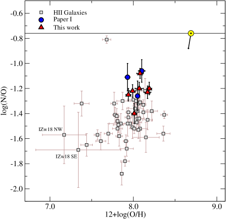
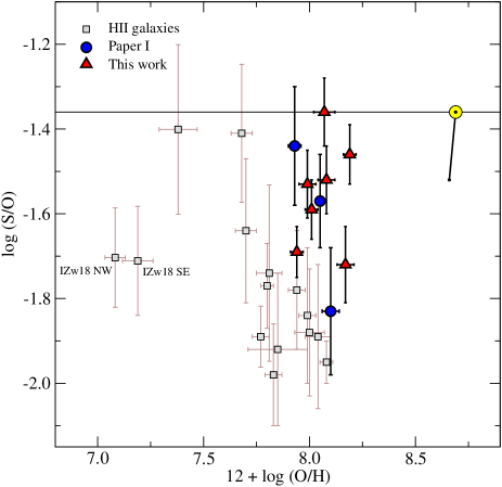
Figure 6: Left panel: N/O ratio as a function of 12+log(O/H) for the observed objects and the objects from Paper I (filled triangles and circles, red and blue respectively in the electronic version of the paper) and the Hii galaxies (open squares) from Table 13. Right panel: same as in the left panel, but for the S/O ratio. The solar values are shown with the usual sun symbol oxygen from Allende-Prieto et al. (2001), nitrogen from Holweger (2001) and sulphur from Grevesse & Sauval (1998). These values are linked by a solid line with the solar ratios from Asplund et al. (2005).

The logarithmic N/O ratios found for the galaxy for which there are T_e([Oii]) and T_e([Nii]) determinations is -1.27$\pm$0.05. If the assumption that t_e([Oii]) = t_e([Nii]) is made, an N/O ratio larger by a factor of 1.5 is obtained. For the rest of the galaxies, for which this assumption has been made, log(N/O) ratios are between -1.40 and -1.20 with an average error of 0.05. For all the objects, the derived values are on the highest side of the distribution for this kind of objects (see Figure 6). In general, the common procedure of obtaining t_e([Oii]) from t_e([Oiii]) using Stasińska’s (1990) relation and assuming t_e([Oii]) = t_e([Nii]), yields N/O ratios larger than using the measured t_e([Oii]) values, since according to Figure 5.1.1, in most cases, the model sequence overpredicts t_e([Oii]). An overprediction of this temperature by a 30 % at T_e([Oii])=13000 K would increase the N/O ratio by a factor of 2. Therefore, the effect of our observed objects showing relatively high N/O ratios seems to be real.

The log(S/O) ratios found for the objects are also listed in table LABEL:total-abs. These values vary between -1.69 and -1.36 with an average error of 0.07, consistent with solar (log(S/O)_⊙ = -1.36) within the observational errors, except for SDSS J1455 and SDSS J1528  for which S/O is lower by a factor of about 1.8. Comparing with the Izotov et al. (2006) derived S/O logarithmic ratios (see Table 12) we find that for three of the observed objects they found S/O ratios lower than ours by us much as 0.4 dex or a factor of about 2.5.

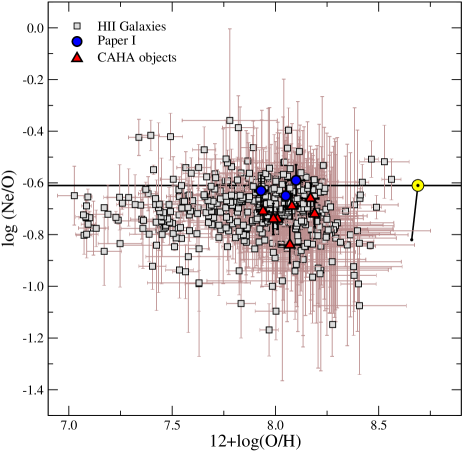
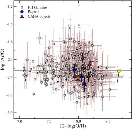
Figure 7: Left panel: Ne/O ratio as a function of 12+log(O/H) for the observed objects and the objects from Paper I (filled triangles and circles, red and blue respectively in the electronic version of the paper) and Hii galaxies (open squares) from Pérez-Montero et al. (2007). Right panel: same as in the left panel, for the Ar/O ratio. The solar values are shown by the usual sun symbol, with oxygen as before and neon and argon from Grevesse & Sauval (1998).

The logarithmic Ne/O ratio varies between -0.84 and -0.66, with a constant value (see Fig. 7) within the errors (table LABEL:total-abs) consistent with solar (log(Ne/O) = 0.61 dex⁵) , if the object with the lowest ratio is excluded. An excellent agreement with the literature values is found.

The values calculated using the classical approximation for the ICF (Ne/O = Ne²⁺/O²⁺), although systematically larger, are within errors very close to those derived using the ICF for neon from Pérez-Montero et al. (2007). This is to be expected, given the high degree of ionization of the objects in the sample.

Finally, the Ar/O ratios found for the observed objects show a larger dispersion than in the case of Ne/O (see Fig. 7), with a mean value consistent with solar⁵. Comparing our estimations for the logarithmic Ar/O ratios with those derived by Izotov et al. (2006), we find a good agreement for three objects, and larger values for SDSS J1509 and SDSS J1540, 0.31 and 0.29 respectively. We must note that for these two objects we have not been able to measure the ionic abundances of Ar³⁺.

Figure 8: Panel (a): log(O⁺/O²⁺) vs. log(S⁺/S²⁺) for the objects in this paper and Paper I (solid red triangles and blue circles respectively) for values calculated using our methodology. Solid diamonds represent the values derived using the conventional method for the same objects (dark green and turquoise respectively in the electronic version of the paper). Open squares are the Hii galaxies from Pérez-Montero & Díaz (2005) with derived oxygen and sulphur ionic ratios. Diagonals in this diagram correspond to constant values of $\eta$. Panel (b): log([Oii]/[Oiii]) vs. log([Sii]/[Siii]), symbols as in panel (a) and the Hii galaxies from Pérez-Montero & Díaz (2005) have data on the [Siii] $\lambda\lambda$ 9069,9532 Å emission lines. Diagonals in this diagram correspond to constant values of $\eta$’.

7.2 Ionisation structure

An insight into the ionisation structure of the observed objects can be gained by means of the O⁺/O²⁺ vs S⁺/S²⁺ diagram (see Paper I).

In panel (a) of Fig. 5.1.1 we show the location on this diagram of the observed objects together with those in Paper I (red filled triangles and blue circles, respectively) and the Hii galaxies in Table 13. In this diagram diagonal lines correspond to constant values of the $\eta$ parameter which can be taken as an indicator of the ionising temperature (Vílchez & Pagel 1988). In this diagram Hii galaxies occupy the region with log $\eta$ between -0.35 and 0.2, which corresponds to high values of the ionising temperature according to these authors. One of the observed objects, SDSS J165712.75+321141.4, shows a very low value of $\eta$=-0.6. This object however, had the [Oii] $\lambda\lambda$ 7319,25 Å affected by atmospheric absorption lines. Unfortunately no previous data of this object exist apart form the SDSS spectrum. We have retrieved this spectrum and measured the [Oii] lines deriving a t_e([Oii]) = 1.23$\pm$0.21, the large error being due to the poor signal to noise in the [Oii] $\lambda$ 7319,25 Å. This lower temperature would increase the value of O⁺/O²⁺ moving the data point corresponding to this objects upwards in the left panel of Figure 5.1.1. This would be consistent with the position of the object in the right panel of the figure which shows log([Oii]/[Oiii]) vs. log([Sii]/[Siii]), the observational equivalent to the $\eta$ plot. The axes in this diagram define log $\eta$’ as:

$$log\,\eta{\textrm{'}}\,=\,log\Big{[}\frac{[O{\textrm{\sc ii}}]\lambda\lambda\,3727,29\,/\,[O{\textrm{\sc iii}}]\lambda\lambda\,4959,5007}{[S{\textrm{\sc ii}}]\lambda\lambda\,6717,31\,/\,[S{\textrm{\sc iii}}]\lambda\lambda\,9069,9532}\Big{]}{}$$

$${}\,=\,log\,\eta-\frac{0.14}{t_{e}}-0.16{}$$

where t_e is the electron temperature in units of 10⁴. The value of log $\eta$’ for SDSS J165712.75+321141.4 is -0.36 corresponding to $\eta$ = -0.09 for t_e([Oiii]) = 1.23.

Inconsistencies between the values of $\eta$ and $\eta$’ are also found if the ionic ratios are derived using values of electron temperatures obtained following the prescriptions given by Izotov et al. (2006). These values are represented by solid diamonds in the left panel of Figure 5.1.1 for the objects in this work and those from paper I. In all cases, higher values of $\eta$ are obtained which, in conjunction with the measured values of $\eta$’, would indicate values of electron temperatures much lower than directly obtained. These higher values of $\eta$ would also imply ionising temperatures lower than those shown by the measured $\eta$’ values.

Metallicity calibrations based on abundances derived according to this conventional method are probably bound to provide metallicities which are systematically too high and should therefore be revised.

8 Summary and conclusions

We have performed a detailed analysis of newly obtained spectra of seven Hii galaxies selected from the Sloan Digital Sky Survey Data Release 3. The spectra cover from 3400 to 10400 Å in wavelength at a FWHM resolution of about 2000 in the blue and 1500 in the red spectral regions.

The high signal-to-noise ratio of the obtained spectra allows the measurement of four line electron temperatures: T_e([Oiii]), T_e([Siii]), T_e([Oii]) and T_e([Sii]), for all the objects of the sample with the addition of T_e([Nii]) for one of the objects. These measurements and a careful and realistic treatment of the observational errors yield total oxygen abundances with accuracies between 7 and 12%. The fractional error is as low as 1% for the ionic O²⁺/H⁺ ratio due to the small errors associated with the measurement of the strong nebular lines of [Oiii] and the derived T_e([Oiii]), but increases to up to 30% for the O⁺/H⁺ ratio. The accuracies are lower in the case of the abundances of sulphur (of the order of 25% for S⁺ and 15% for S²⁺) due to the presence of larger observational errors both in the measured line fluxes and the derived electron temperatures. The error for the total abundance of sulphur is also larger than in the case of oxygen (between 15% and 20%) due to the uncertainties in the ionisation correction factors.

This is in contrast with the unrealistically small errors quoted for line temperatures other than T_e([Oiii]) in the literature, in part due to the commonly assumed methodology of deriving them from the measured T_e([Oiii]) through a theoretical relation. These relations are found from photoionization model sequences and no uncertainty is attached to them although large scatter is found when observed values are plotted; usually the line temperatures obtained in this way carry only the observational error found for the T_e([Oiii]) measurement and does not include the observed scatter, thus heavily understimating the errors in the derived temperature.

In fact, no clear relation is found between T_e([Oiii]) and T_e([Oii]) for the existing sample of objects confirming our previous results. A comparison between measured and model derived T_e([Oii]) shows than, in general, model predictions overestimate this temperature and hence underestimate the O⁺/H⁺ ratio. This, though not very important for high excitation objects, could be of some concern for lower excitation ones for which total O/H abundances could be underestimated by up to 0.2 dex. It is worth noting that the objects observed with double-arm spectrographs, therefore implying simultaneous and spatially coincident observations over the whole spectral range, show less scatter in the T_e([Oiii]) - T_e([Oii] plane clustering around the N_e = 100 cm^-3 photo-ionisation model sequence. On the other hand, this small scatter could partially be due to the small range of temperatures shown by these objects due to possible selection effects. This small temperature range does not allow either to investigate the metallicity effects found in the ralations between the various line temperatures in recent photo-ionisation models by Izotov et al. (2006).

Also, the observed objects, as well as those in Paper I, though showing Ne/O and Ar/O relative abundances typical of those found for a large Hii galaxy sample (Pérez-Montero et al. 2007), show higher than typical N/O abundance ratios that would be even higher if the [Oii] temperatures would be found from photo-ionisation models. We therefore conclude that approach of deriving the O⁺ temperature from the O²⁺ one should be discouraged if an accurate abundance derivation is sought.

These issues could be addressed by re-observing the objects in Table 13 , which cover an ample range in temperatures and metal content, with double arm spectrographs. This sample should be further extended to obtain a self consistent sample of about 50 objects with high S/N and excellent spectrophotometry covering simultaneously from 3600 to 9900 Å This simple and easily feasible project would provide important scientific return in the form of critical tests of photoionisation models.

The O⁺/O²⁺ and S⁺/S²⁺ ratios for all the observed galaxies, except one, cluster around a value of the “softness parameter” $\eta$ of 1 implying high values of the stellar ionising temperature. For the discrepant object, showing a much lower value of $\eta$, the intensity of the [Oii] $\lambda\lambda$ 7319,25 Å lines are affected by atmospheric absorption lines. When the observational counterpart of the ionic ratios is used, this object shows a ionisation structure similar to the rest of the observed ones. This simple exercise shows the potential of checking for consistency in both the $\eta$ and $\eta$’ plots in order to test if a given assumed ionisation structure is adequate. In fact, these consistency checks show that the stellar ionising temperatures found for the observed Hii galaxies using the ionisation structure predicted by state of the art ionisation models result too low when compared to those implied by the corresponding observed emission line ratios. Therefore, metallicity calibrations based on abundances derived according to this conventional method are probably bound to provide metallicities which are systematically too high and should be revised.

Acknowledgements

We wish to express our gratitude to Fabian Rosales for calculating the ionic He abundances for our objects using Porter’s Helium emissivities. We are pleased to thank the staff at Calar Alto, and especially Felipe Hoyo, for their assistance during the observations. We also thank the Time Allocation Committee for awarding observing time and an anonymous referee for her/his careful and constructive revision of the manuscript.

Funding for the creation and distribution of the SDSS Archive has been provided by the Alfred P. Sloan Foundation, the Participating Institutions, the National Aeronautics and Space Administration, the National Science Foundation, the US Department of Energy, the Japanese Monbukagakusho, and the Max Planck Society. The SDSS Web site is http://www.sdss.org.

The SDSS is managed by the ARC for the Participating Institutions. The Participating Institutions are the University of Chicago, Fermilab, the Institute for Advanced Study, the Japan Participation Group, The Johns Hopkins University, the Korean Scientist Group, Los Alamos National Laboratory, the Max Planck Institute for Astronomy (MPIA), the Max Planck Institute for Astrophysics (MPA), New Mexico State University, the University of Pittsburgh, the University of Portsmouth, Princeton University, the United States Naval Observatory, and the University of Washington.

This research has made use of the NASA/IPAC Extragalactic Database (NED) which is operated by the Jet Propulsion Laboratory, California Institute of Technology, under contract with the National Aeronautics and Space Administration and of the SIMBAD database, operated at CDS, Strasbourg, France.

This work has been partially supported by DGICYT grant AYA-2004-02860-C03. GH and MC acknowledge support from the Spanish MEC through FPU grants AP2003-1821 and AP2004-0977. AID acknowledges support from the Spanish MEC through a sabbatical grant PR2006-0049. Also, partial support from the Comunidad de Madrid under grant S-0505/ESP/000237 (ASTROCAM) is acknowledged. PM acknowledges support from CNRS-INSU (France) and its Programme National Galaxies. Support from the Mexican Research Council (CONACYT) through grant 19847-F is acknowledged by ET and RT. We thank the hospitality of the Institute of Astronomy of Cambridge where part of this paper was developed. GH and MC also thank the hospitality of the INAOE and the Laboratoire d’Astrophysique de Toulouse-Tarbes.

When we mentioned to Bernard Pagel the title of this paper he said, with his characteristic cheeky grin: “precision abundance? but that’s an oxymoron. It will be nice if you can do it”. Dear Bernard, you are sadly missed; we dedicate this work to your memory.

References

- Adelman-McCarthy & for the SDSS Collaboration (2007) Adelman-McCarthy J. K., for the SDSS Collaboration 2007, ArXiv e-prints, astro-ph0707.3413
- Allende-Prieto et al. (2001) Allende-Prieto C., Lambert D. L., Asplund M., 2001, Astrophys. J. Letters, 556, L63
- Asplund et al. (2005) Asplund M., Grevesse N., Sauval A. J., 2005, in Barnes III T. G., Bash F. N., eds, Cosmic Abundances as Records of Stellar Evolution and Nucleosynthesis Vol. 336 of Astronomical Society of the Pacific Conference Series, The Solar Chemical Composition. pp 25–+
- Baldwin et al. (1981) Baldwin J. A., Phillips M. M., Terlevich R., 1981, Publ. Astron. Soc. Pac., 93, 5
- Barker (1980) Barker T., 1980, Astrophys. J., 240, 99
- Benjamin et al. (1999) Benjamin R. A., Skillman E. D., Smits D. P., 1999, Astrophys. J., 514, 307
- Butler & Zeippen (1994) Butler K., Zeippen C. J., 1994, Astron. and Astrophys. Suppl. Sries, 108, 1
- de Robertis et al. (1987) de Robertis M. M., Dufour R. J., Hunt R. W., 1987, Royal Astronomical Society of Canada, Journal, 81, 195
- Díaz (1988) Díaz A. I., 1988, Mon. Not. R. Astron. Soc., 231, 57
- Ferland et al. (1998) Ferland G. J., Korista K. T., Verner D. A., Ferguson J. W., Kingdon J. B., Verner E. M., 1998, Publ. Astron. Soc. Pac., 110, 761
- French (1980) French H. B., 1980, Astrophys. J., 240, 41
- Galavis et al. (1995) Galavis M. E., Mendoza C., Zeippen C. J., 1995, Astron. and Astrophys. Suppl. Sries, 111, 347
- Garnett (1992) Garnett D. R., 1992, Astron. J., 103, 1330
- González-Delgado et al. (2005) González-Delgado R. M., Cerviño M., Martins L. P., Leitherer C., Hauschildt P. H., 2005, Mon. Not. R. Astron. Soc., 357, 945
- González-Delgado et al. (1994) González-Delgado R. M., Pérez E., Tenorio-Tagle G., Vílchez J. M., Terlevich E., Terlevich R., Telles E., Rodríguez-Espinosa J. M., Mas-Hesse M., García-Vargas M. L., Díaz A. I., Cepa J., Castañeda H., 1994, Astrophys. J., 437, 239
- Grevesse & Sauval (1998) Grevesse N., Sauval A. J., 1998, Space Science Reviews, 85, 161
- Guseva et al. (2000) Guseva N. G., Izotov Y. I., Thuan T. X., 2000, Astrophys. J., 531, 776 (GIT00)
- Hägele et al. (2006) Hägele G. F., Pérez-Montero E., Díaz A. I., Terlevich E., Terlevich R., 2006, Mon. Not. R. Astron. Soc., 372, 293 (Paper I)
- Holweger (2001) Holweger H., 2001, in Wimmer-Schweingruber R. F., ed., Joint SOHO/ACE workshop ”Solar and Galactic Composition” Vol. 598 of American Institute of Physics Conference Series, Photospheric Abundances: Problems, Updates, Implications. pp 23–+
- Hoyos & Díaz (2006) Hoyos C., Díaz A. I., 2006, Mon. Not. R. Astron. Soc., 365, 454
- Izotov et al. (2001) Izotov Y. I., Chaffee F. H., Schaerer D., 2001, Astron. Astrophys., 378, L45 (ICS01)
- Izotov et al. (2004) Izotov Y. I., Stasińska G., Guseva N. G., Thuan T. X., 2004, Astron. Astrophys., 415, 87 (IT04)
- Izotov et al. (2006) Izotov Y. I., Stasińska G., Meynet G., Guseva N. G., Thuan T. X., 2006, Astron. Astrophys., 448, 955
- Izotov & Thuan (1998) Izotov Y. I., Thuan T. X., 1998, Astrophys. J., 500, 188 (IT98)
- Izotov et al. (1994) Izotov Y. I., Thuan T. X., Lipovetsky V. A., 1994, Astrophys. J., 435, 647 (ITL94)
- Izotov et al. (1997) Izotov Y. I., Thuan T. X., Lipovetsky V. A., 1997, Astrophys. J., Suppl. Ser., 108, 1 (ITL97)
- Kehrig et al. (2006) Kehrig C., Vílchez J. M., Telles E., Cuisinier F., Pérez-Montero E., 2006, Astron. Astrophys., 457, 477
- Kingdon & Ferland (1995) Kingdon J., Ferland G. J., 1995, Astrophys. J., 442, 714
- Kniazev et al. (2004) Kniazev A. Y., Pustilnik S. A., Grebel E. K., Lee H., Pramskij A. G., 2004, Astrophys. J., Suppl. Ser., 153, 429
- Koo et al. (1995) Koo D. C., Guzmán R., Faber S. M., Illingworth G. D., Bershady M. A., Kron R. G., Takamiya M., 1995, Astrophys. J. Letters, 440, L49
- Kunth & Sargent (1983) Kunth D., Sargent W. L. W., 1983, Astrophys. J., 273, 81
- Lee et al. (2004) Lee J. C., Salzer J. J., Melbourne J., 2004, Astrophys. J., 616, 752 (L04)
- Lennon & Burke (1994) Lennon D. J., Burke V. M., 1994, Astron. and Astrophys. Suppl. Sries, 103, 273
- Liu et al. (2000) Liu X.-W., Storey P. J., Barlow M. J., Danziger I. J., Cohen M., Bryce M., 2000, Mon. Not. R. Astron. Soc., 312, 585
- López (2005) López J., 2005, MSc Thesis. INAOE
- Melbourne et al. (2004) Melbourne J., Phillips A., Salzer J. J., Gronwall C., Sarajedini V. L., 2004, Astron. J., 127, 686 (M04)
- Miller & Mathews (1972) Miller J. S., Mathews W. G., 1972, Astrophys. J., 172, 593
- Olive & Skillman (2001) Olive K. A., Skillman E. D., 2001, New Astronomy, 6, 119
- Olive & Skillman (2004) Olive K. A., Skillman E. D., 2004, Astrophys. J., 617, 29
- Pagel et al. (1992) Pagel B. E. J., Simonson E. A., Terlevich R. J., Edmunds M. G., 1992, Mon. Not. R. Astron. Soc., 255, 325
- Pauldrach et al. (2001) Pauldrach A. W. A., Hoffmann T. L., Lennon M., 2001, Astron. Astrophys., 375, 161
- Peimbert & Costero (1969) Peimbert M., Costero R., 1969, Boletin de los Observatorios Tonantzintla y Tacubaya, 5, 3
- Peimbert & Torres-Peimbert (1992) Peimbert M., Torres-Peimbert S., 1992, Astron. Astrophys., 253, 349
- Pérez-Montero & Díaz (2003) Pérez-Montero E., Díaz A. I., 2003, Mon. Not. R. Astron. Soc., 346, 105 (PMD03)
- Pérez-Montero & Díaz (2005) Pérez-Montero E., Díaz A. I., 2005, Mon. Not. R. Astron. Soc., 361, 1063
- Pérez-Montero et al. (2006) Pérez-Montero E., Díaz A. I., Vílchez J. M., Kehrig C., 2006, Astron. Astrophys., 449, 193
- Pérez-Montero et al. (2007) Pérez-Montero E., Hägele G. F., Contini T., Díaz A. I., 2007, Mon. Not. R. Astron. Soc.(in press)
- Porter et al. (2005) Porter R. L., Bauman R. P., Ferland G. J., MacAdam K. B., 2005, Astrophys. J. Letters, 622, L73
- Pradhan (1976) Pradhan A. K., 1976, Mon. Not. R. Astron. Soc., 177, 31
- Ramsbottom et al. (1996) Ramsbottom C. A., Bell K. L., Stafford R. P., 1996, Atomic Data and Nuclear Data Tables, 63, 57
- Rodríguez & Rubin (2004) Rodríguez M., Rubin R. H., 2004, in IAU Symp. 217, Recycling Intergallactic and Interstellar Matter, ed. P. A. Duc, J. Braine, and E. Brinks (San Francisco: ASP) The Ionization Equilibrium of Iron in HII Regions. pp 188–+ (astro–ph/0312246)
- Rosa-González et al. (2007) Rosa-González D., Schmitt H. R., Terlevich E., Terlevich R., 2007, Astrophys. J., 654, 226
- Sargent & Searle (1970) Sargent W. L. W., Searle L., 1970, Astrophys. J. Letters, 162, L155+
- Searle & Sargent (1972) Searle L., Sargent W. L. W., 1972, Astrophys. J., 173, 25
- Shaw & Dufour (1995) Shaw R. A., Dufour R. J., 1995, Publ. Astron. Soc. Pac., 107, 896
- Skillman & Kennicutt (1993) Skillman E. D., Kennicutt Jr. R. C., 1993, Astrophys. J., 411, 655 (SK93)
- Skillman et al. (1994) Skillman E. D., Televich R. J., Kennicutt Jr. R. C., Garnett D. R., Terlevich E., 1994, Astrophys. J., 431, 172 (S94)
- Stasińska (1978) Stasińska G., 1978, Astron. Astrophys., 66, 257
- Stasińska (1990) Stasińska G., 1990, Astron. and Astrophys. Suppl. Sries, 83, 501
- Storey & Hummer (1995) Storey P. J., Hummer D. G., 1995, Mon. Not. R. Astron. Soc., 272, 41
- Stoughton & et al. (2002) Stoughton C., et al. 2002, Astron. J., 123, 485
- Tayal & Gupta (1999) Tayal S. S., Gupta G. P., 1999, Astrophys. J., 526, 544
- Terlevich et al. (1991) Terlevich R., Melnick J., Masegosa J., Moles M., Copetti M. V. F., 1991, Astron. and Astrophys. Suppl. Sries, 91, 285 (T91)
- Vílchez & Pagel (1988) Vílchez J. M., Pagel B. E. J., 1988, Mon. Not. R. Astron. Soc., 231, 257
- Zeippen et al. (1987) Zeippen C. J., Le Bourlot J., Butler K., 1987, Astron. Astrophys., 188, 251