Abstract

We describe the development of Analytic Perturbation Theory (APT) in QCD, called Fractional APT (FAPT), which has been suggested to apply the renormalization group evolution and QCD factorization technique in the framework of APT.

1 Basics of APT in QCD

In the standard QCD Perturbation Theory (PT) we have:

• the Renormalization Group (RG) equation $da_{s}(L)/dL=-a_{s}^{2}-c_{1}\,a_{s}^{3}-\ldots$ for the effective coupling $\alpha_{s}(\mu^{2})=(4\pi/b_{0})\,a_{s}(L)$ with $L=\ln(\mu^{2}/\Lambda^{2})$;

• the one-loop solution generates Landau pole singularity: $a_{s}(L)=1/L$;

• the two-loop solution generates square-root singularity: $a_{s}(L)\sim 1/\sqrt{L+c_{1}\ln c_{1}}$;

• PT series is a series in powers of effective coupling: $D(L)=1+d_{1}a_{s}(L)+d_{2}a_{s}^{2}(L)+\ldots$

In the Analytic Perturbation Theory (APT) we have:

• different effective couplings in Minkowskian (Radyushkin [1], and Krasnikov and Pivovarov [2]) and Euclidean (Shirkov and Solovtsov [3]) regions;

• APT is based on the RG and causality that guaranties standard perturbative UV asymptotics and spectral properties;

• in Euclidean domain, $\displaystyle-q^{2}=Q^{2}$, $\displaystyle L=\ln Q^{2}/\Lambda^{2}$, APT generates the following set of images for the effective coupling and its $n$-th powers, $\displaystyle\left\{{\cal A}_{n}(L)\right\}_{n\in\mathbb{N}}$;

• in Minkowskian domain, $\displaystyle q^{2}=s$, $\displaystyle L_{s}=\ln s/\Lambda^{2}$, APT generates another set of images for the effective coupling and its $n$-th powers, $\displaystyle\left\{{\mathfrak{A}}_{n}(L_{s})\right\}_{n\in\mathbb{N}}$;

• PT power series $\displaystyle\sum\limits_{m}d_{m}a_{s}^{m}(Q^{2})$ transforms into non-power series $\displaystyle\sum\limits_{m}d_{m}{\cal A}_{m}(Q^{2})$ in APT, where $d_{m}$ are numbers in $\overline{\text{MS}\vphantom{{}^{1}}}$ -scheme.

By the analytization in APT for an observable $f(Q^{2})$ we mean the “Källen–Lehman” representation

$$\left[f(Q^{2})\right]_{\text{an}}=\int_{0}^{\infty}\!\frac{\rho_{f}(\sigma)}{\sigma+Q^{2}-i\epsilon}\,d\sigma$$ (1)

with the spectral density $\rho_{f}(\sigma)=\textbf{Im}\,\big{[}f(-\sigma)\big{]}/\pi$. Then in the one-loop approximation (note pole remover $(e^{L}-1)^{-1}$ in (2))

$${\cal A}_{1}(Q^{2}) = \int_{0}^{\infty}\!\frac{\rho(\sigma)}{\sigma+Q^{2}}\,d\sigma\ =\ \frac{1}{L}-\frac{1}{e^{L}-1}\,,~{}$$ (2)

$${\mathfrak{A}}_{1}(s) = \int_{s}^{\infty}\!\frac{\rho(\sigma)}{\sigma}\,d\sigma\ =\ \frac{1}{\pi}\,\arccos\frac{L_{s}}{\sqrt{\pi^{2}+L_{s}^{2}}}\,,~{}$$ (3)

whereas analytic images of the higher powers ($n\geq 2,n\in\mathbb{N}$) are:

$$\!\!\!\!{\cal A}_{n}(Q^{2})\!\! \!=\!\! \!\!\int_{0}^{\infty}\!\frac{\rho_{n}(\sigma)}{\sigma+Q^{2}}\,d\sigma\!=\!\frac{1}{(n-1)!}\left(-\frac{d}{dL}\right)^{n-1}\!\!\!\!\!{\cal A}_{1}(L)\,,~{}$$ (4)

$${\mathfrak{A}}_{n}(s)\!\! \!=\!\! \!\!\int_{s}^{\infty}\!\frac{\rho_{n}(\sigma)}{\sigma}\,d\sigma\!=\!\frac{1}{(n-1)!}\left(-\frac{d}{dL}\right)^{n-1}\!\!\!\!\!{\mathfrak{A}}_{1}(L)\,.$$ (5)

2 Problems of APT and their resolution in FAPT

In the standard QCD PT we have not only power series $F(L)=\sum\limits_{m}f_{m}\,a_{s}^{m}(L)$, but also:

• the factorization procedure in QCD gives rise to the appearance of logarithmic factors of the type: $a_{s}^{\nu}(L)\,L$; 

• the RG evolution generates evolution factors of the type: $B(Q^{2})=\left[Z(Q^{2})/Z(\mu^{2})\right]\,B(\mu^{2})$, which reduce in the one-loop approximation to $Z\sim a_{s}^{\nu}(L)$ with $\nu=\gamma_{0}/(2b_{0})$ being a fractional number;

• the RG in the two-loop approximation for the coupling $\displaystyle\to\left[a_{s}(L)\right]^{\nu}\ln\left(a_{s}(L)\right)$.

That means we need to think how to obtain analytization of new functions: $\displaystyle\left(a_{s}\right)^{\nu},\ \left(a_{s}\right)^{\nu}\ln(a_{s})$, $\displaystyle\left(a_{s}\right)^{\nu}L^{m}$, $\ldots$ .

Let us first do it for the one-loop APT. Here we have a very nice recursive relation (2). We will use it to construct analytic images of fractional powers of QCD effective coupling in the Euclidean (FAPT) and Minkowskian (MFAPT) domains. Consider the Laplace transform

$${{\cal A}_{1}(L)\choose{\mathfrak{A}}_{1}(L)}=\int_{0}^{\infty}\!{\tilde{{\cal A}}_{1}(t)\choose{\mathfrak{A}}_{1}(t)}\,e^{-Lt}dt\,,$$ (6)

which is well defined for all $L>0$. Then

$${{\cal A}_{n}(L)\choose{\mathfrak{A}}_{n}(L)}=\int_{0}^{\infty}\!{\tilde{{\cal A}}_{1}(t)\choose{\mathfrak{A}}_{1}(t)}\left[\frac{t^{n-1}}{(n-1)!}\right]\,e^{-Lt}dt\,.$$ (7)

Moreover, we can define for all $\nu\in\mathbb{R}$

$${{\cal A}_{\nu}(L)\choose{\mathfrak{A}}_{\nu}(L)}=\int_{0}^{\infty}\!{\tilde{{\cal A}}_{1}(t)\choose{\mathfrak{A}}_{1}(t)}\left[\frac{t^{\nu-1}}{(\nu-1)!}\right]\,e^{-Lt}dt\,.$$ (8)

The only things one needs to know are $\tilde{{\cal A}}_{1}(t)$ and $\tilde{{\mathfrak{A}}}_{1}(t)$. Eqs. (2) and (3) produce the answer: $\displaystyle\tilde{{\cal A}}_{1}(t)=1-\sum_{m=1}^{\infty}\delta(t-m)$ and $\displaystyle\tilde{{\mathfrak{A}}}_{1}(t)=\left[\frac{\textbf{sin}\pi t}{\pi t}\right]$. This allows us to obtain explicit expressions for ${\cal A}_{\nu}(L)$ ($L=\ln Q^{2}/\Lambda^{2}$) and ${\mathfrak{A}}_{\nu}(L)$ ($L=\ln s/\Lambda^{2}$) using Eq. (8):

$${\cal A}_{\nu}(L)=\frac{1}{L^{\nu}}-\frac{F(e^{-L},1-\nu)}{\Gamma(\nu)}\,;\quad{\mathfrak{A}}_{\nu}(L)=\frac{\text{sin}\left[(\nu-1)\arccos\left(L/\sqrt{\pi^{2}+L^{2}}\right)\right]}{\pi(\nu-1)\left(\pi^{2}+L^{2}\right)^{(\nu-1)/2}}\,.~{}$$ (9)

Here $F(z,\nu)$ is reduced Lerch transcendental function. It is an analytic function in $\nu$. Interesting to note that ${\cal A}_{\nu}(L)$ appears to be an entire function in $\nu$, whereas ${\mathfrak{A}}_{\nu}(L)$ is determined completely in terms of elementary functions. These expressions can be analytically continued to negative values of $L$, though in derivation we assume $L>0$.

Let us discuss the main properties of ${\cal A}_{\nu}(L)$ ($L=\ln Q^{2}/\Lambda^{2}$) and ${\mathfrak{A}}_{\nu}(L)$ ($L=\ln s/\Lambda^{2}$):

   

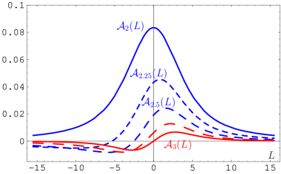
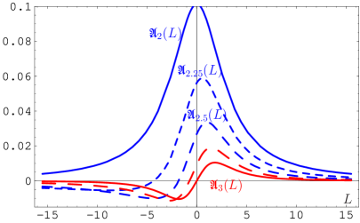
Figure 1: Graphics of ${\cal A}_{\nu}(L)$ (left panel) and ${\mathfrak{A}}_{\nu}(L)$ (right panel) for fractional $\nu\in\left[2,3\right]$.

These couplings have the following properties:
➊ $\displaystyle{\cal A}_{0}(L)={\mathfrak{A}}_{0}(L)=1\vphantom{{}^{\int}_{|}}$;
➋ $\displaystyle{\cal A}_{-m}(L)=L^{m}$ for $m\in\mathbb{N}$;  $\displaystyle{\mathfrak{A}}_{-1}(L)=L$,  $\displaystyle{\mathfrak{A}}_{-2}(L)=L^{2}-\frac{\pi^{2}}{3}$,  $\displaystyle{\mathfrak{A}}_{-3}(L)=L^{3}-\pi^{2}L\,,\,\ldots\vphantom{{}^{\int}_{|}}$;
➌ $\displaystyle{{\cal A}_{m}(L)\vphantom{{}^{\int}}\choose{\mathfrak{A}}_{m}(L)\vphantom{{}_{|}}}\!\!=\!\!(-1)^{m}{{\cal A}_{m}(-L)\choose{\mathfrak{A}}_{m}(-L)}$ for $m\geq 2\,,m\in\mathbb{N}$;
➍ $\displaystyle{\cal A}_{m}(\pm\infty)={\mathfrak{A}}_{m}(\pm\infty)=0$ for $m\geq 2\,,\ m\in\mathbb{N}\vphantom{{}^{\int}_{\big{|}}}$;
➎ $\displaystyle{\cal D}^{k}{{\cal A}_{\nu}\vphantom{{}^{\int}}\choose{\mathfrak{A}}_{\nu}\vphantom{{}_{|}}}\equiv\frac{d^{k}}{d\nu^{k}}{{\cal A}_{\nu}\choose{\mathfrak{A}}_{\nu}}=\left[\frac{d^{k}}{d\nu^{k}}a^{\nu}\right]_{\text{an}}=\left[a^{\nu}\ln^{k}(a)\right]_{\text{an}}$;
➏ $\displaystyle{\cal A}_{\nu}(L)=\frac{-1}{\Gamma(\nu)}\sum_{r=0}^{\infty}\zeta(1-\nu-r)\frac{(-L)^{r}}{r!}\vphantom{{}^{\int}_{|}}$ for $|L|\!<\!2\pi$. The convergence of this expansion is very fast.

   

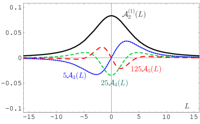
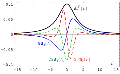
Figure 2: Graphics of ${\cal A}_{\nu}(L)$ (left panel) and ${\mathfrak{A}}_{\nu}(L)$ (right panel) for integer $\nu=2,3,4,5$. In order to show all curves on the same panel we scale different curves by factors $5^{\nu-2}$.

We display graphics of ${\cal A}_{\nu}(L)$ and ${\mathfrak{A}}_{\nu}(L)$ in Fig. 1: one can see here a kind of distorting mirror on both panels. Next, in Fig. 2 we show graphics for $\nu=2,3,4,5$. Here we can trace the partial values

$${\cal A}_{2}(0)=\frac{1}{12}\,,~{}~{}{\cal A}_{4}(0)=\frac{-1}{720}\,,~{}~{}{\cal A}_{3}(0)={\cal A}_{5}(0)=0\,;~{}~{}$$

$${\mathfrak{A}}_{2}(0)=\frac{1}{\pi^{2}}\,,~{}~{}{\mathfrak{A}}_{4}(0)=-\frac{1}{3\pi^{4}}\,,~{}~{}{\mathfrak{A}}_{3}(0)={\mathfrak{A}}_{5}(0)=0\,.$$

Graphics for ${\cal A}_{\nu}(L)$ as functions of $\nu$ at fixed values of $L$ can be found in our last papers [5]. We compare the basic ingredients of (M)FAPT in Table 1 with their counterparts in conventional PT and APT.

Table 1: Comparison of PT, APT, FAPT ($\displaystyle L=\ln\left(Q^{2}/\Lambda^{2}\right)$), and MFAPT ($\displaystyle L=\ln\left(s/\Lambda^{2}\right)$). In the row, named ‘Inverse powers’, we put ${\mathfrak{A}}_{-m}(L)=L^{m}+O(\pi^{2})$ that symbolically encodes just the item (2) of ${\mathfrak{A}}_{\nu}(L)$ properties, see the list on the previous page.

Theory	PT	APT	FAPT	MFAPT
Space	$\Big{\{}a^{\nu}\Big{\}}_{\nu\in\mathbb{R}}\vphantom{{}^{\big{|}}_{\big{|}}}$	$\Big{\{}{\cal A}_{m}\Big{\}}_{m\in\mathbb{N}}$	$\Big{\{}{\cal A}_{\nu}\Big{\}}_{\nu\in\mathbb{R}}$	$\Big{\{}{\mathfrak{A}}_{\nu}\Big{\}}_{\nu\in\mathbb{R}}$
Series expansion	$\sum\limits_{m}f_{m}\,a^{m}(L)\vphantom{{}^{\big{|}}_{\big{|}}}$	$\sum\limits_{m}f_{m}\,{\cal A}_{m}(L)$	$\sum\limits_{m}f_{m}\,{\cal A}_{m}(L)$	$\sum\limits_{m}f_{m}\,{\mathfrak{A}}_{m}(L)$
Inverse powers	$\left(a(L)\right)^{-m}\vphantom{{}^{\big{|}}_{\big{|}}}$	—	${\cal A}_{-m}(L)=L^{m}$	${\mathfrak{A}}_{-m}(L)=L^{m}+O(\pi^{2})$
Index derivative	$a^{\nu}\ln^{{k}}{a}\vphantom{{}^{\big{|}}_{\big{|}}}$	—	${\cal D}^{k}{\cal A}_{\nu}$	${\cal D}^{k}\,{\mathfrak{A}}_{\nu}$

3 Development of (M)FAPT: Two-loop coupling

The two-loop equation for the normalized coupling $a=b_{0}\,\alpha/(4\pi)$ is

$$\frac{da_{(2)}(L)}{dL}=-a_{(2)}^{2}(L)\left[1+c_{1}\,a_{(2)}(L)\right]\quad\text{with}~{}c_{1}\equiv\frac{b_{1}}{b_{0}^{2}}\,.$$ (10)

   

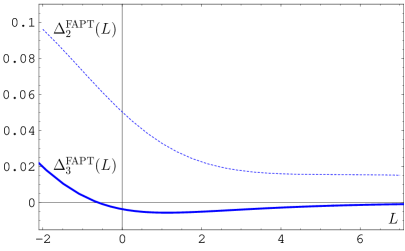
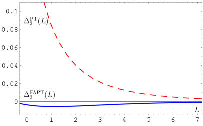
Figure 3: Left panel: Comparison of relative errors $\Delta_{2}^{\text{FAPT}}(L)$ (dotted line) and $\Delta_{3}^{\text{FAPT}}(L)$ (solid line) in FAPT. Right panel: Comparison of relative errors $\Delta_{3}^{\text{PT}}(L)$ (dashed line) in standard PT and $\Delta_{3}^{\text{FAPT}}(L)$ (solid line) in FAPT.

RG solution of this equation assumes the following form:

$$\frac{1}{a_{(2)}(L)}+c_{1}\ln\left[\frac{a_{(2)}(L)}{1+c_{1}a_{(2)}(L)}\right]=L=\frac{1}{a_{(1)}(L)}\,.$$ (11)

We can expand $a_{(2)}(L)$ in terms of $a_{(1)}(L)=1/L$ with inclusion of terms ${\cal O}(a_{(1)}^{3})$:

$$a_{(2)}(L)=a_{(1)}(L)+c_{1}\,a_{(1)}^{2}(L)\,\ln\,a_{(1)}(L)+c_{1}^{2}\,a_{(1)}^{3}(L)\left(\ln^{2}a_{(1)}(L)+\ln\,a_{(1)}(L)-1\right)+\ldots\,.$$

Analytic version of this expansion is

$$\!\!\!{\cal A}_{1}^{(2);\text{FAPT}}(L) = {\cal A}_{1}^{(1)}+c_{1}\,{\cal D}\,{\cal A}_{\nu=2}^{(1)}+c_{1}^{2}\left({\cal D}^{2}+{\cal D}-1\right){\cal A}_{\nu=3}^{(1)}+\ldots\,.$$

In Fig. 3 we demonstrate nice convergence of this expansion using relative errors of the 2- and 3-term approximations:

$$\Delta_{2}^{\text{FAPT}}(L) = 1-\frac{{\cal A}_{1}^{(1)}(L)+c_{1}\,{\cal D}{\cal A}_{\nu=2}^{(1)}(L)}{{\cal A}_{1}^{(2)}(L)}\,;$$

$$\Delta_{3}^{\text{FAPT}}(L) = \Delta_{2}^{\text{FAPT}}(L)-\frac{c_{1}^{2}\,\left({\cal D}^{2}+{\cal D}-1\right)\,{\cal A}_{\nu=3}^{(1)}(L)}{{\cal A}_{1}^{(2)}(L)}\,;$$

$$\Delta_{3}^{\text{PT}}(L)=1-\frac{a_{(1)}(L)+c_{1}\,a_{(1)}^{2}(L)\,\ln\,a_{(1)}(L)+c_{1}^{2}\,a_{(1)}^{3}(L)\left(\ln^{2}a_{(1)}(L)+\ln\,a_{(1)}(L)-1\right)}{a_{(2)}(L)}\,.$$

We see that relative accuracy of the 3-term approximation in FAPT (see the left panel of Fig. 3) is better than 2% for $L\geq-2$. In the same time, the right panel of Fig. 3 demonstrates that relative accuracy of the same 3-term approximation in standard PT even at $L\approx 1$ is much higher — about 10%, whereas in FAPT it is smaller than 1%!

We can also obtain the corresponding expansion for the two-loop coupling with index $\nu$:

$$\!\!\!{\cal A}_{\nu}^{(2);\text{FAPT}}(L) = {\cal A}_{\nu}^{(1)}(L)+c_{1}\nu\,{\cal D}\,{\cal A}_{\nu+1}^{(1)}(L)+c_{1}^{2}\nu\left[\frac{\nu+1}{2}{\cal D}^{2}\!+\!{\cal D}\!-\!1\right]\!{\cal A}_{\nu+2}^{(1)}(L)+\ldots\,.~{}~{}~{}$$ (12)

and display comparison of different results for ${\cal A}_{2}^{(2);\text{FAPT}}(L)$ on the left panel of Fig. 4. On the right panel of this figure we show comparison of FAPT and standard QCD PT with respect to the fractional index (power) of the coupling, fixed at the value $\nu=0.62$.

   

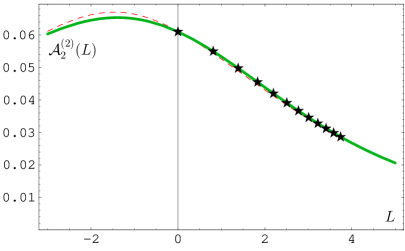
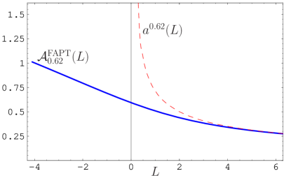
Figure 4: Left panel: The solid line corresponds to ${\cal A}_{2}^{(2)}(L)$, computed analytically via Eq. (12); dashed line represents the result of a numerical integration, while stars correspond to the available numerical results of Magradze in [6]. Right panel: The solid line represents ${\cal A}_{0.62}^{(2);\text{FAPT}}(L)$, computed analytically via Eq. (12), while the dashed line stands for $a^{0.62}_{(2)}(L)$.

In Minkowskian region convergence of MFAPT expansion for the two-loop coupling

$$\!\!\!{\mathfrak{A}}_{2}^{(2);\text{MFAPT}}(L) = {\mathfrak{A}}_{2}^{(1)}(L)+2\,c_{1}\,{\cal D}\,{\mathfrak{A}}_{\nu=3}^{(1)}(L)+c_{1}^{2}\,\left[3\,{\cal D}^{2}+2\,{\cal D}-2\right]\!{\mathfrak{A}}_{\nu=4}^{(1)}(L)+\ldots\,.~{}~{}~{}$$ (13)

is also nice, but in the vicinity of the point $L=0$ (Landau pole in the standard PT) it is not so fast, so that we need to take into account $O(c_{1}^{5})$-terms in order to reach 5% level of accuracy, for more details look in [5].

4 Electromagnetic pion form factor at NLO

Scaled hard-scattering amplitude truncated at the next-to-leading order (NLO) and evaluated at renormalization scale $\mu_{R}^{2}=\lambda_{R}Q^{2}$ reads [7, 8, 9, 10]

$$T^{\text{NLO}}_{H}\left(x,y;\mu_{F}^{2},Q^{2}\right)=\frac{\alpha_{s}\left(\lambda_{R}Q^{2}\right)}{Q^{2}}\,t_{H}^{(0)}(x,y)+\frac{\alpha_{s}^{2}\left(\lambda_{R}Q^{2}\right)}{4\pi\,Q^{2}}\,t_{H}^{(1)}(x,y;{\mu_{F}^{2}}/{Q^{2}})~{}~{}~{}$$ (14)

with shorthand notation ($\bar{x}\equiv 1-x$)

$$~{}~{}t_{H}^{(1)}(x,y;{\mu_{F}^{2}}/{Q^{2}})=\left[C_{F}\,t_{\text{H}}^{(0)}\left(x,y\right)\left[2\Big{(}3+\ln\,(\bar{x}\bar{y})\Big{)}\ln\frac{Q^{2}}{\mu_{F}^{2}}\right]+b_{0}\,t_{H}^{(1,\beta)}\left(x,y;\lambda_{R}\right)+t_{H}^{(\text{FG})}(x,y)\right]\,.$$

The leading twist-2 pion distribution amplitude (DA) [11] at normalization scale $\mu_{F}^{2}$ is given by [12]

$$\varphi_{\pi}(x,\mu_{F}^{2})=6\,x\,(1-x)\left[1+a_{2}(\mu_{F}^{2})\,C_{2}^{3/2}(2x-1)+a_{4}(\mu_{F}^{2})\,C_{4}^{3/2}(2x-1)+\ldots\,\right]\,.$$

All nonperturbative information is encapsulated in Gegenbauer coefficients $a_{n}(\mu^{2}_{F})$.

To obtain factorized part of pion form factor (FF) one needs to convolute the pion DA with the hard-scattering amplitude:

$$F_{\pi}^{\text{Fact}}(Q^{2})=\varphi_{\pi}(x;\mu_{F}^{2})\mathop{\otimes}\limits_{x}T^{\text{NLO}}_{H}\left(x,y;\mu_{F}^{2},Q^{2}\right)\mathop{\otimes}\limits_{y}\varphi_{\pi}(y;\mu_{F}^{2})\,.$$

In order to obtain the analytic expression for the pion FF at NLO in [13, 14] the so-called “Naive Analytization” has been suggested. It uses analytic image only for coupling itself, ${\cal A}_{1}^{(2)}$, but not for its powers. In contrast and in full accord with the APT ideology the receipt of “Maximal Analytization” has been proposed recently in [15]. The corresponding expressions for the analytized hard amplitudes read as follows:

$$\left[Q^{2}T_{H}\left(x,y,Q^{2}\right)\right]_{\text{Nai-An}} = {\cal A}_{1}^{(2)}(\lambda_{R}Q^{2})\,t_{H}^{(0)}(x,y)+\frac{\left({\cal A}_{1}^{(2)}(\lambda_{R}Q^{2})\right)^{2}}{4\pi}\,t_{H}^{(1)}\left(x,y;\lambda_{R},\frac{\mu_{F}^{2}}{Q^{2}}\right)\,;$$

$$\left[Q^{2}T_{H}\left(x,y,Q^{2}\right)\right]_{\text{Max-An}} = {\cal A}_{1}^{(2)}(\lambda_{R}Q^{2})\,t_{H}^{(0)}(x,y)+\frac{{\cal A}_{2}^{(2)}(\lambda_{R}Q^{2})}{4\pi}\,t_{H}^{(1)}\left(x,y;\lambda_{R},\frac{\mu_{F}^{2}}{Q^{2}}\right)\,.$$

  

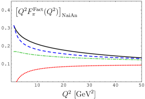
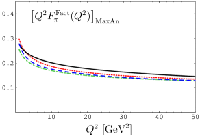
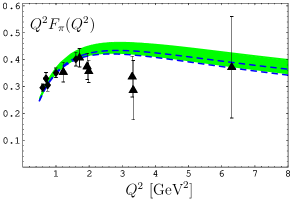
Figure 5: Left panel: Factorized pion FF in the “Naive Analytization”. Central panel: Factorized pion FF in the “Maximal Analytization”. On both panels solid lines correspond to the scale setting $\mu_{R}^{2}=1$ GeV², dashed lines — to $\mu_{R}^{2}=Q^{2}$, dotted lines — to the BLM prescription, whereas dash-dotted lines — to the $\alpha_{v}$-scheme. Right panel: Predictions for the scaled pion form factor calculated with the BMS bunch of the pion DAs. The dashed lines inside the strip indicate the corresponding area of predictions obtained with the asymptotic pion DA. The experimental data are taken from [16] (diamonds) and [17], [18] (triangles).

In Fig. 5 we show the predictions for the factorized pion FF in the “Naive” and in the “Maximal Analytization” approaches. We see that in the “Maximal Analytization” approach the obtained results are practically insensitive to the renormalization scheme and scale-setting choice (already at the NLO level).

We show also the graphics for the whole pion FF, obtained in APT with the “Maximally Analytic” procedure using the Ward identity to match the non-factorized and factorized parts of the pion FF, see the right panel of Fig. 5. The green strip in this figure contains both nonperturbative uncertainties from nonlocal QCD sum rules [19, 20, 21] and renormalization scheme and scale ambiguities at the level of the NLO accuracy.

It is interesting to note here that FAPT approach, used in [22] for analytization of the $\ln(Q^{2}/\mu_{F}^{2})$-terms in the hard amplitude (14), diminishes also the dependence on the factorization scale setting in the interval $\mu_{F}^{2}=1-10$ GeV².

5 Concluding Remarks

We conclude with the following resume:
① The implementation of the analyticity concept (the dispersion relations) from the level of the coupling and its powers to the level of QCD amplitudes as a whole generates extension of the APT to (M)FAPT ;
② We formulate the rules how to apply (M)FAPT at the two- and three-loop levels;
③ We show that convergence of the perturbative expansion is significantly improved when using non-power ( M)FAPT expansion;
④ As an additional advantage we obtain the minimal sensitivity to both the renormalization and factorization scale setting, revealed on the example of the pion electromagnetic form factor.

Acknowledgments: This investigation was supported in part by the Deutsche Forschungsgemeinschaft (Projects DFG 436 RUS 113/881/0), the Heisenberg–Landau Programme, grant 2007, the Russian Foundation for Fundamental Research, grants No. 05-01-00992 and 07-02-91557, and the BRFBR–JINR Cooperation Programme, contract No. F06D-002.

References

[1]
A. V. Radyushkin,
JINR Rapid Commun. 78, 96 (1996).
[2]
N. V. Krasnikov and A. A. Pivovarov,
Phys. Lett. B116, 168 (1982).
[3]
D. V. Shirkov and I. L. Solovtsov,
JINR Rapid Commun. 2[76], 5 (1996);
Phys. Rev. Lett. 79, 1209 (1997).
[4]
A. I. Karanikas, N. G. Stefanis,
Phys. Lett. B 504 (2001) 225;
ibid. B 636 (2006) 330.
[5]
A. P. Bakulev, S. V. Mikhailov, and N. G. Stefanis,
Phys. Rev. D72, 074014 (2005);
Phys. Rev. D75, 056005 (2007).
[6]
B. A. Magradze,
Preprint RMI-2003-55, 2003 [hep-ph/0305020].
[7]
R. D. Field, R. Gupta, S. Otto, and L. Chang,
Nucl. Phys. B186, 429 (1981).
[8]
F. M. Dittes and A. V. Radyushkin,
Sov. J. Nucl. Phys. 34, 293 (1981).
[9]
E. Braaten and S.-M. Tse,
Phys. Rev. D35, 2255 (1987).
[10]
B. Melić, B. Nižić, and K. Passek,
Phys. Rev. D60, 074004 (1999).
[11]
A. V. Radyushkin,
Dubna preprint P2-10717, 1977 [hep-ph/0410276].
[12]
A. V. Efremov and A. V. Radyushkin,
Phys. Lett. B94, 245 (1980).
[13]
N. G. Stefanis, W. Schroers, and H.-C. Kim,
Phys. Lett. B449, 299 (1999).
[14]
N. G. Stefanis, W. Schroers, and H.-C. Kim,
Eur. Phys. J. C18, 137 (2000).
[15]
A. P. Bakulev, K. Passek-Kumerički, W. Schroers, and N. G. Stefanis,
Phys. Rev. D70, 033014 (2004).
[16]
J. Volmer et al.,
Phys. Rev. Lett. 86, 1713 (2001).
[17]
C. N. Brown et al.,
Phys. Rev. D8, 92 (1973).
[18]
C. J. Bebek et al.,
Phys. Rev. D13, 25 (1976).
[19]
A. P. Bakulev, S. V. Mikhailov, and N. G. Stefanis,
Phys. Lett. B508, 279 (2001);
in Proceedings of the 36th Rencontres De Moriond
On QCD And Hadronic Interactions, 17–24 Mar 2001, Les Arcs, France,
edited by J. T. T. Van (World Scientific, Singapore, 2002), pp. 133–136;
Phys. Rev. D67, 074012 (2003);
Phys. Lett. B578, 91 (2004).
[20]
A. P. Bakulev and A. V. Pimikov,
Acta Phys. Polon. B37, 3627 (2006);
PEPAN Lett. 4, 637 (2007);
Int. J. Mod. Phys. A22, 654 (2007).
[21]
A. P. Bakulev,
in New Trends in High-Energy Physics,
Proceedings of the Conference, Yalta (Crimea), 16–23 Sept., 2006,
edited by P. N. Bogolyubov, L. L. Jenkovszky, V. V. Magas, and Z. I. Vakhnenko
(BITP NASU (Kiev), JINR (Dubna), Kiev, 2006), pp. 203–212.
[22]
A. P. Bakulev, A. I. Karanikas, and N. G. Stefanis,
Phys. Rev. D72, 074015 (2005).