Spectral density of an interacting dot coupled indirectly to conducting leads

Abstract

We study the spectral density of electrons $\rho_{d\sigma}(\omega)$ in an interacting quantum dot (QD) with a hybridization $\lambda$ to a non-interacting QD, which in turn is coupled to a non-interacting conduction band. The system corresponds to an impurity Anderson model in which the conduction band has a Lorentzian density of states of width $\Delta_{2}$. We solved the model using perturbation theory in the Coulomb repulsion $U$ (PTU) up to second order and a slave-boson mean-field approximation (SBMFA). The PTU works surprisingly well near the exactly solvable limit $\Delta_{2}\longrightarrow 0$. For fixed $U$ and large enough $\lambda$ or small enough $\Delta_{2}$, the Kondo peak in $\rho_{d\sigma}(\omega)$ splits into two peaks. This splitting can be understood in terms of weakly interacting quasiparticles. Before the splitting takes place the universal properties of the model in the Kondo regime are lost. Using the SBMFA, simple analytical expressions for the occurrence of split peaks are obtained. For small or moderate $\Delta_{2}$, the side bands of $\rho_{d\sigma}(\omega)$ have the form of narrow resonances, that were missed in previous studies using the numerical renormalization group. This technique also has shortcomings for describing properly the split Kondo peaks. As the temperature is increased, the intensity of the split Kondo peaks decreases, but it is not completely suppressed at high temperatures.

I Introduction

The quantum impurity models, like the Kondo and Anderson ones have attracted the solid state physics community due to their complex and rich behavior as well as due to their applications to many strongly correlated physical systems.hew In recent years, the attention into these models has increased due to the advances in nanotechnology, which for example made it possible to build ideal ”single impurity” systems with one quantum dot (QD) in which the Kondo physics was clearly displayed gold1 ; cro ; gold2 ; wiel confirming predictions based on the Anderson model.glaz ; ng ; chz . In other fascinating experiments, quantum corrals assembled by depositing a close line of atoms or molecules on Cu or noble metal (111) surfaces have been used to “project” the Kondo effect to a remote place.man The Anderson model used to describe these systems has the additional complication of the particular structure of the non-interacting states, which cannot be described by a constant density of states.rev However, it has been shown that the non-interacting Green’s function can be written as a discrete sum of simple fractions.mir ; hvar

More recently, systems of several impurities or QD’s have become a subject of great interest. For example non-trivial results for the spectral density were observed when three Cr atoms are placed on the (111) surface of Au.jamn ; trimer Systems of two,jeong ; craig ; chen three,waugh ; gaud and more kouw QD’s have been assembled to study the effects of interdot hopping on the Kondo effect, and other physical properties driven by strong correlations. Particular systems have been proposed theoretically as realizations of the two-channel Kondo model,oreg ; zit the so called ionic Hubbard model,ihm and the double exchange mechanism.mart In the last years, transport through arrays of a few QD’s corn ; zit2 ; ogur ; nisi ; 3do and spin qubits in double QD’s sq have been studied theoretically.

Last year, Dias da Silva et al. dias proposed a system with one interacting QD (1) with a hopping term $\lambda$ to another non-interacting QD (2), which in turn is hybridized with conducting leads. This hybridization is in principle larger than the charging energy of QD 2, in such a way that the latter can be considered as non interacting. The model is equivalent to an impurity Anderson model in which the conduction band has a Lorentzian density of states of width $\Delta_{2}$. This is one of the simplest variations of the model in which the effects of a non trivial structure of the conduction band can be studied. It can also be regarded as the simplification of the Anderson model used to describe the quantum mirage rev ; mir ; hvar ; ali or a tight binding model for a ring with a quantum dot rev ; pc when only the resonance at the Fermi energy is included. This simplification is qualitatively valid when the separation in energy between resonances is larger than their width. In the case of a constant density of conduction states and on-site energy $E_{d}$ below the Fermi energy $\epsilon_{F}$, for large enough Coulomb repulsion $U$, the spectral density of the impurity shows two broad peaks (called charge transfer peaks) at $E_{d}<\epsilon_{F}$ and $E_{d}+U>\epsilon_{F}$, and another peak near $\epsilon_{F}$ (the Kondo peak).

Previous calculations of the spectral density of the impurity in the model for the quantum mirage mir ; ali ; wily and in confined structures corna have shown that the Kondo peak near the Fermi energy splits in two for certain parameters. Dias da Silva et al. studied the spectral density at the QD 1 $\rho_{d\sigma}(\omega)$ and magnetic susceptibility of the symmetric model using numerical renormalization group (NRG). In agreement with previous studies, they find that when $\lambda$ increases beyond a certain critical value $\lambda_{c}$, the Kondo resonance splits. In a similar way, for large enough $\lambda$ split peaks are observed if $U$ is smaller than a critical value $U_{c}$. In fact previous calculations for the spectral density of an impurity inside a circular corral show split peaks in the non-interacting case $U=0$ that turn into one peak as $U$ is increased.hvar The splitting condition is proposed to correspond approximately to the equality $\sqrt{2}T_{K}=\Delta_{2}$, where $T_{K}$ is the Kondo temperature. However, the results presented to support this reasonable statement are limited. The spectral density is shown only for three particular sets of parameters. Moreover, the ability of the NRG to describe peaks far from the Fermi energy might be questionable because due to the logarithmic discretization, the resolution at a given energy $\omega$ is proportional to $\omega-\epsilon_{F}$. In addition, the spectral broadening affects the resolution.bulla

In this paper we use perturbation theory in the Coulomb repulsion $U$ (PTU) up to second order yos ; hor and a slave-boson mean-field approximation (SBMFA) kr to study in more detail the spectral density, the conditions for the appearance of split peaks near $\epsilon_{F}$, and the evolution of the energy scale $T_{K}$ with the parameters of the model. We also compare with exact results in the limit $\Delta_{2}\rightarrow 0$, and derived from the Friedel sum rule.lan As explained in the next section, both approximations take a simpler form in the symmetric Anderson model considered, and the PTU works better in this case, allowing us to describe new physics, and obtain reasonably robust results with comparatively simple mathematics.

For the SBMFA we used a straightforward extension of the method proposed by Kotliar and Ruckenstein to the Hubbard model.kr

The paper is organized as follows. The model, the approximations (PTU and SBMFA) and some exact results derived from Fermi liquid properties and the case $\Delta_{2}=0$ are presented in Section II. Several figures illustrating the main results are presented in Section III. Section IV is a short summary and discussion.

II Hamiltonian, approximations and exact results

II.1 Model and equations for the spectral density

The system is described by the following Hamiltonian:

$$H=H_{1}+H_{2}+H_{l}+H_{\lambda}+H_{V},$$ (1)

where $H_{1}$ ($H_{2}$) describes the interacting (non-interacting) QD, $H_{l}$ the leads, and the last two terms are the hybridization of the non-interacting QD with the interacting one and the leads respectively. In standard notation

$$H_{1} = E_{d}\sum_{\sigma}d_{\sigma}^{\dagger}d_{\sigma}+Ud_{\uparrow}^{\dagger}d_{\uparrow}d_{\downarrow}^{\dagger}d_{\downarrow},$$

$$H_{2} = \epsilon_{a}\sum_{\sigma}a_{\sigma}^{\dagger}a_{\sigma},\text{ }H_{l}=\sum_{l\sigma}\epsilon_{l}c_{l\sigma}^{\dagger}c_{l\sigma},$$

$$H_{\lambda} = \lambda\sum_{\sigma}(d_{\sigma}^{\dagger}a_{\sigma}+\text{H.c.}),$$

$$H_{V} = \sum_{l\sigma}W_{l}(a_{\sigma}^{\dagger}c_{l\sigma}+\text{H.c.}).$$ (2)

The sum $H_{2}+H_{l}+H_{V}$ is a non-interacting Hamiltonian which can be put in the diagonal form $\sum_{k\sigma}\epsilon_{k}c_{k\sigma}^{\dagger}c_{k\sigma}$ by means of a canonical transformation. In this basis the Hamiltonian takes the form of the impurity Anderson model for a general band structure and hybridization

$$H=H_{1}+\sum_{k\sigma}\epsilon_{k}c_{k\sigma}^{\dagger}c_{k\sigma}+\sum_{k\sigma}V_{k}(d_{\sigma}^{\dagger}c_{k\sigma}+\text{H.c.}),$$ (3)

where $V_{k}=\lambda\{a_{\sigma},c_{k\sigma}^{\dagger}\}$.

The spectral density of electrons at the interacting QD is

$$\rho_{d\sigma}(\omega)=\frac{1}{2\pi}[G_{dd\sigma}(\omega-i\eta)-G_{dd\sigma}(\omega+i\eta)],$$ (4)

where $\eta$ is a positive infinitesimal and calling $z=\omega+i\eta$ ($z=\omega-i\eta$), the retarded (advanced) Green’s function at the interacting QD can be written in the form mir ; lan

$$G_{dd\sigma}(z)=\frac{1}{z-E_{d}-\Sigma_{sd\sigma}(z)-\Sigma_{dd\sigma}(z)},$$ (5)

where $\Sigma_{dd\sigma}(z)$ is the self-energy due to the interaction $U$ and

$$\Sigma_{sd\sigma}(z)=\sum_{k}\frac{|V_{k}|^{2}}{z-\epsilon_{k}}.$$ (6)

While this result holds for a general Hamiltonian of the form (3), for the particular case of Eqs. (1) and (2), using equations of motion,mir it can be shown that dias

$$\Sigma_{sd\sigma}(z)=\lambda^{2}G_{aa\sigma}^{0}(z),$$ (7)

where $G_{aa\sigma}^{0}(z)$ is the Green’s function of the non-interacting QD in the absence of the interacting one (for a Hamiltonian $H_{2}+H_{l}+H_{V}$). The model assumes constant values for the matrix element $W_{l}$ and the density of states of the leads $\rho$.dias These assumptions are usually very good approximations for the range of energies of interest in QD’s. Calling $\Delta_{2}=\pi\rho|W|^{2}$, they lead to

$$G_{aa\sigma}^{0}(\omega\pm i\eta)=\frac{1}{\omega-\epsilon_{a}\pm i\Delta_{2}}.$$ (8)

In the following, as in Ref. dias, , we take the origin of one-particle energies at the Fermi energy ($\epsilon_{F}=0$), and take $\epsilon_{a}=0$, $\epsilon_{d}=-U/2$, corresponding to the symmetric Anderson model. In summary, the model is equivalent to an impurity Anderson model with the hybridization function

$$\Delta(\omega)=-\mathrm{Im}\Sigma_{sd\sigma}(\omega+i\eta)=\frac{\lambda^{2}\Delta_{2}}{\omega^{2}+\Delta_{2}^{2}}.$$ (9)

Note that in general, the real part of $\Sigma_{sd\sigma}$ can be obtained from the relation

$$\Lambda(\omega)=\mathrm{Re}\Sigma_{sd\sigma}(\omega)=P\int\frac{\Delta(\epsilon)d\epsilon}{\pi(\omega-\epsilon)}$$ (10)

If some approximation for $\Sigma_{dd\sigma}(z)$ is used, the above equations (4), (5), (7) and (8) define the spectral density.

II.2 Approximations

II.2.1 Perturbations in $U$

The starting point of the perturbation theory in $U$ (PTU) is a non-interacting problem which includes some one-body potential so that the effective on-site energy of the interacting electrons $E_{d}$ is modified to $E_{d\sigma}^{eff}$. A possible choice is the Hartree-Fock value $E_{d\sigma}^{eff}=E_{d}+U\langle d_{\bar{\sigma}}^{\dagger}d_{\bar{\sigma}}\rangle$. This one-body potential is compensated in the perturbation, which includes it (with the opposite sign) in addition to the interaction term $Ud_{\uparrow}^{\dagger}d_{\uparrow}d_{\downarrow}^{\dagger}d_{\downarrow}$. In general, there are better choices for $E_{d\sigma}^{eff}$ which have been used recently in several calculations of transport properties in nanoscopic systems, including non-equilibrium situations and applied magnetic fields.none However, for the symmetric Anderson model at equilibrium without applied magnetic field (for which $\langle d_{\sigma}^{\dagger}d_{\sigma}\rangle=1/2$) these choices coincide with the Hartree-Fock result and $E_{d\sigma}^{eff}=E_{d}+U/2=\epsilon_{F}$. In this case, for a flat band the theory is quantitatively correct up to $U\sim 8\Delta$, where $\Delta$ is the resonant level width.silver ; dots Working up to order $U^{2}$ we can write yos ; hor ; mir

$$[G_{dd\sigma}(z)]^{-1}=[g_{dd\sigma}(z)]^{-1}-\Sigma_{dd\sigma}^{(2)}(z),$$ (11)

where $g_{dd\sigma}(z)$ is the Green’s function for the interaction treated in Hartree-Fock (including contributions of first order in $U$ to $\Sigma_{dd\sigma}$)

$$g_{dd\sigma}(z)=\frac{1}{z-\Sigma_{sd\sigma}(z)},$$ (12)

and $\Sigma_{dd\sigma}^{(2)}(z)$ is the contribution to the self-energy of second order in $U$ evaluated from a Feynman diagram involving the analytical extension of the time ordered $g_{dd\sigma}$ to Matsubara frequencies

$$\Sigma_{dd\sigma}^{(2)}(i\omega_{l},T) = U^{2}T\sum_{m}g_{dd\sigma}(i\omega_{l}-i\nu_{m})\chi_{\bar{\sigma}}(i\nu_{m}),$$ (13)

$$\chi_{\sigma}(i\nu_{m}) = -T\sum_{n}g_{dd\sigma}(i\omega_{n})g_{dd\sigma}(i\omega_{n}+i\nu_{m}),$$ (14)

where $\omega_{n}=(2n+1)\pi T$ and $\nu_{m}=2m\pi T$.

Our task is simplified because $\chi_{\sigma}$ can be calculated analytically due to the fact that $g_{dd\sigma}$ can be expressed as a sum of two simple fractions

$$g_{dd\sigma}(\omega+i\eta)=\frac{\omega+i\Delta_{2}}{\omega^{2}+i\Delta_{2}\omega-\lambda^{2}}=\sum_{l=1}^{2}\frac{a_{l}}{\omega-r_{l}+i\delta_{l}}.$$ (15)

This is the retarded Green’s function. In order to evaluate perturbative diagrams, like Eqs. (13), (14), one needs the analytical extension of the time ordered Green function to imaginary frequencies $\omega\rightarrow i\omega_{n}$ mahan ; mir :

$$g_{dd\sigma}(i\omega_{n})=\sum_{l}\frac{a_{l}+\overline{a_{l}}+(a_{l}-\overline{a_{l}})\text{sgn}(\omega_{n})}{2\left[i\omega_{n}+i\delta_{l}\text{sgn}(\omega_{n})-r_{l}\right]},$$ (16)

where $\overline{a_{l}}$ is the complex conjugate of $a_{l}$ and sgn$(x)$ is the sign of $x$.

The sums over Matsubara frequencies, Eqs. (13), (14) have been done in Ref. mir, . The latter can be expressed in terms of the digamma function $\Psi(z)$.abra The final result for the retarded quantities is

$$\Sigma_{dd\sigma}^{(2)}(\omega) = \frac{U^{2}}{\pi}\int_{-\infty}^{\infty}dy\ [\frac{1}{e^{y/T}-1}g_{dd\sigma}(\omega-y)\mathrm{Im}\chi_{\bar{\sigma}}(y)+$$ (17)

$$+\frac{1}{e^{y/T}+1}\mathrm{Im}g_{dd\sigma}(-y)\ \chi_{\bar{\sigma}}(\omega+y)],$$

where

$$\chi_{\sigma}(\omega) = -\frac{i}{2\pi}\ \sum_{lm}\left(A_{lm}(\omega)-B_{lm}(\omega)\right)\Psi_{l}(0)+$$ (18)

$$+\left(\overline{B_{lm}}(-\omega)-\overline{A_{lm}}(-\omega)\right)\overline{\Psi_{l}}(0)$$

$$-\left(B_{lm}(\omega)+A_{lm}(-\omega)\right)\Psi_{l}(\omega)$$

$$-\left(\overline{B_{lm}}(-\omega)+\overline{A_{lm}}(\omega)\right)\overline{\Psi_{l}}(-\omega),$$

with

$$A_{lm}(\omega) = \frac{a_{l}\ a_{m}}{\omega+r_{l}-r_{m}-i\delta_{l}+i\delta_{m}},$$

$$B_{lm}(\omega) = \frac{a_{l}\ \overline{a_{m}}}{\omega-r_{l}+r_{m}+i\delta_{l}+i\delta_{m}},$$

$$\Psi_{l}(\omega) = \Psi\left(\frac{1}{2}+\frac{\delta_{l}+i(r_{l}-\omega)}{2\pi T}\right).$$ (19)

Eqs. (4), (7), (8), (11), (12) and (17) to (19) define the spectral density of the interacting dot within PTU.

II.2.2 Slave bosons

The basic idea of the slave boson formalism of Kotliar and Ruckenstein kr is to enlarge the Fock space to include bosonic states which correspond to each state in the fermionic description at the interacting QD. The vacuum state at this site is represented as $e^{\dagger}\left|0\right\rangle$, where $e^{\dagger}$ is a bosonic creation operator corresponding to the empty QD; similarly $s_{\sigma}^{\dagger}f_{\sigma}^{\dagger}\left|0\right\rangle$ represents the singly occupied state $d_{\sigma}^{\dagger}\left|0\right\rangle$, where $s_{\sigma}^{\dagger}$ is a bosonic operator for singly occupied sites with spin $\sigma$, and $f_{\sigma}^{\dagger}$ is a fermion operator. The doubly occupied site $d_{\uparrow}^{\dagger}d_{\downarrow}^{\dagger}\left|0\right\rangle$ is represented as $b^{\dagger}f_{\uparrow}^{\dagger}f_{\downarrow}^{\dagger}\left|0\right\rangle$ In this way the interaction term can be expressed in terms of boson operators as $Ub^{\dagger}b$ and the interactions between fermions disappear from the Hamiltonian. In other words, the fermion operator $d_{\sigma}^{\dagger}$ is expressed in terms of fermion operators that do not interact between them as $d_{\sigma}^{\dagger}=(b^{\dagger}s_{\bar{\sigma}}+s_{\sigma}^{\dagger}e)f_{\sigma}^{\dagger}$. The bosonic operators should satisfy the following constraints

$$e^{\dagger}e+\sum_{\sigma}s_{\sigma}^{\dagger}s_{\sigma}+b^{\dagger}b = 1$$

$$s_{\sigma}^{\dagger}s_{\sigma}+b^{\dagger}b = f_{\sigma}^{\dagger}f_{\sigma}.$$ (20)

Introducing Lagrange multipliers for these constraints, the Hamiltonian takes the form

$$H = H_{2}+H_{l}+H_{V}+E_{d}\sum_{\sigma}f_{\sigma}^{\dagger}f_{\sigma}+Ub^{\dagger}b$$ (21)

$$+\lambda\sum_{\sigma}\left[R_{\sigma}(b^{\dagger}s_{\bar{\sigma}}+s_{\sigma}^{\dagger}e)L_{\sigma}f_{\sigma}^{\dagger}a_{\sigma}+\text{H.c.}\right]$$

$$+\mu_{\sigma}(s_{\sigma}^{\dagger}s_{\sigma}+b^{\dagger}b-f_{\sigma}^{\dagger}f_{\sigma})$$

$$-\mu(e^{\dagger}e+\sum_{\sigma}s_{\sigma}^{\dagger}s_{\sigma}+b^{\dagger}b-1).$$

Here, the factors

$$R_{\sigma} = (1-e^{\dagger}e-s_{\sigma}^{\dagger}s_{\sigma})^{-1/2}\ ,$$

$$L_{\sigma} = (1-s_{\sigma}^{\dagger}s_{\sigma}-b^{\dagger}b)^{-1/2},$$ (22)

are equivalent to one when treated exactly, but they are introduced in such a way that in the slave-boson mean-field approximation (SBMFA) the correct result in the non-interacting case is reproduced.

In the SBMFA, all the boson operators are replaced by numbers and the free energy is minimized with respect to them. In the symmetric Anderson model, without applied magnetic field the problem simplifies considerably. In this case $s^{2}$ is independent of spin and $e^{2}=b^{2}$. Also $\langle d_{\sigma}^{\dagger}d_{\sigma}\rangle=\langle f_{\sigma}^{\dagger}f_{\sigma}\rangle=1/2$. From here $E_{d}-\mu_{\sigma}=\epsilon_{F}=0$ and using Eqs. (20) $s^{2}=1/2-b^{2}$ and only one independent variable remains. Also $R_{\sigma}=L_{\sigma}=\sqrt{2}$. The change in free energy due to the impurity can be written as hew ; 3do

$$\Delta F=-\frac{2}{\pi}\mathrm{Im}\int_{-\infty}^{+\infty}f(\omega)\ln G_{ff\sigma}(\omega+i\eta)\ d\omega\ +Ub^{2}$$

$$+2\mu_{\sigma}(s^{2}+b^{2}),$$ (23)

where $f(\omega)$ is the Fermi function and $G_{ff\sigma}(\omega)$ is the Green’s function of the $f$ operators for any spin. The Hamiltonian takes the same form as that of a non-interacting problem with $E_{d}=\epsilon_{F}=0$ and renormalized hopping $\tilde{\lambda}=R_{\sigma}(b^{\dagger}s_{\bar{\sigma}}+s_{\sigma}^{\dagger}e)L_{\sigma}\lambda$, that in our case simplifies to

$$\tilde{\lambda}=4b\sqrt{1/2-b^{2}}\lambda.$$ (24)

Then, as in the previous subsection

$$G_{ff\sigma}(\omega+i\eta)=\frac{\omega+i\Delta_{2}}{\omega^{2}+i\Delta_{2}\omega-\tilde{\lambda}^{2}}.$$ (25)

Decomposing this expression in simple fractions [as in Eq. (15)] and replacing in Eq. (23), the integral can be evaluated analytically at zero temperature. The result should be separated in two cases depending on the sign of $2\tilde{\lambda}-\Delta_{2}$. Except for irrelevant constants, the result is

$$\Delta F = \frac{\Delta_{2}}{\pi}\{\ln(1+r^{2})+r(2\arctan r^{-1}-\pi)\}+Ub^{2}\text{ }$$

$$\text{for }x \geq 1\text{, and}$$

$$\Delta F = \frac{\Delta_{2}}{\pi}\{(1-r)\ln(1-r)+(1+r)\ln(1+r)\}+Ub^{2},$$

$$\text{for }x \leq 1\text{, with}$$

$$r = \sqrt{|x^{2}-1|},\text{ }x=2\tilde{\lambda}/\Delta_{2}.$$ (26)

Minimizing $\Delta F$ defined by Eqs. (26) and (24), one obtains a transcendental equation for $b$. After solving this, a characteristic energy scale or Kondo temperature can be defined by the gain in energy with respect to the unhybridized case:

$$T_{K}=\Delta F(\tilde{\lambda}_{\min})-\Delta F(0),$$ (27)

where $\tilde{\lambda}_{\min}$ is the value of $\tilde{\lambda}$ evaluated with Eq. (24) for the value of $b$ that minimizes the energy.

The spectral density for real $d$ electrons near the Fermi energy becomes, using $d_{\sigma}^{\dagger}=R_{\sigma}(b^{\dagger}s_{\bar{\sigma}}+s_{\sigma}^{\dagger}e)L_{\sigma}f_{\sigma}^{\dagger}$ in the SBMFA

$$G_{dd\sigma}(\omega+i\eta)\simeq(\tilde{\lambda}_{\min}/\lambda)^{2}G_{ff\sigma}(\omega+i\eta).$$ (28)

In the resulting spectral density $\rho_{d\sigma}(\omega)$ [calculated from Eq. (4)], the “charge transfer” peaks near $E_{d}$ and $E_{d}+U$ are lost, as explained in more detail in the next section.

From the change of sign of $\partial^{2}\rho_{d\sigma}(\omega)/\partial\omega^{2}$ evaluated at the Fermi energy, one finds that (in a similar way as in the non-interacting case dias ) the critical condition for the appearance or disappearance of split peaks near the Fermi energy is

$$\sqrt{2}\tilde{\lambda}_{\min}=\Delta_{2}\text{.}$$ (29)

Combining this equation with Eq. (24) and the minimization condition $\partial\Delta F/\partial b=0$, we find in order to have split peaks, it is necessary that $\lambda>\Delta_{2}/\sqrt{2}$ and that $U<U_{c}$, where

$$U_{c}=\frac{8\lambda^{2}}{\Delta_{2}}\left(1-\frac{\Delta_{2}^{2}}{2\lambda^{2}}\right)^{1/2}.$$ (30)

This analytical result can be inverted to give the minimum value of $\lambda$ required to have split peaks for fixed $U$ and $\Delta_{2}:$

$$\lambda_{c}=\frac{U}{4\left(\left(1+\frac{U^{2}}{4\Delta_{2}^{2}}\right)^{1/2}-1\right)^{1/2}}.$$ (31)

II.3 Exact results

II.3.1 Fermi liquid properties

It is known that at the Fermi energy, the imaginary part of the self energy due to interaction vanishes in a Fermi liquid.lutt Using $\mathrm{Im}\Sigma_{dd\sigma}(\epsilon_{F})=0$, and Eqs. (4) and (5) with $\Sigma_{sd\sigma}(\omega\pm i\eta)=\Lambda_{\sigma}(\omega)\mp i\Delta_{\sigma}(\omega)$, the spectral density at the Fermi energy can be written in the form

$$\rho_{d\sigma}(\epsilon_{F})=\frac{\cos^{2}\varphi_{\sigma}}{\pi\Delta_{\sigma}(\epsilon_{F})},$$ (32)

where

$$\varphi_{\sigma}=\arctan\left(\frac{E_{d}+\Sigma_{dd\sigma}(\epsilon_{F})+\Lambda_{\sigma}(\epsilon_{F})}{\Delta_{\sigma}(\epsilon_{F})}\right).$$ (33)

In addition, for the general Anderson model, the Friedel sum rule is valid lan

$$\varphi_{\sigma}=\pi\left(\langle d_{\sigma}^{\dagger}d_{\sigma}\rangle-\frac{1}{2}\right)$$

$$+\mathrm{Im}\int_{-\infty}^{\epsilon_{F}}d\omega G_{dd\sigma}(\omega+i\eta)\frac{\partial\Sigma_{sd\sigma}(\omega+i\eta)}{\partial\omega}.$$ (34)

As explained below, for the symmetric Anderson model without applied magnetic field, with the choice $\epsilon_{F}=0$, it can be shown that the real (imaginary) part of $G_{dd\sigma}(\omega+i\eta)$ is odd (even). Then Eq. (5) implies $\mathrm{Re}[E_{d}+\Sigma_{sd\sigma}(0)+\Sigma_{dd\sigma}(0)]=0$. From Eq. (33) $\varphi_{\sigma}=0$ and from Eq. (32)

$$\rho_{d\sigma}(0)=\frac{1}{\pi\Delta(0)}.$$ (35)

The symmetry properties of $G_{dd\sigma}(\omega+i\eta)$ can be demonstrated using the Lehman representation of the Green’s function mahan and the fact that the symmetric Anderson model is invariant under the transformation $T:d_{\sigma}^{\dagger}\rightarrow d_{\sigma}$, $c_{\mathbf{k}\sigma}^{\dagger}\rightarrow-c_{\mathbf{k}^{\prime}\sigma}$, with $\epsilon_{\mathbf{k}^{\prime}}=-\epsilon_{\mathbf{k}}$. Calling $\Omega$ the thermodynamic potential and $|n\rangle$ a complete set of eigenstates, we can write mahan

$$G_{dd\sigma}(\omega+i\eta)=e^{\beta\Omega}\sum_{n,m}|\langle n|d_{\sigma}^{\dagger}|m\rangle|^{2}\frac{e^{-\beta E_{n}}+e^{-\beta E_{m}}}{\omega+E_{n}-E_{m}+i\eta}.$$ (36)

Because of symmetry one has $\langle n|d_{\sigma}^{\dagger}|m\rangle=\langle Tn|Td_{\sigma}^{\dagger}T^{\dagger}|Tm\rangle$ $=\langle Tn|d_{\sigma}|Tm\rangle$ $=\overline{\langle Tm|d_{\sigma}^{\dagger}|Tn\rangle}$, and the eigenstates $|m\rangle$ and $|Tm\rangle$ have the same energy. Then changing the labels of the sum above $|n\rangle$ by $|Tm\rangle$ and $|m\rangle$ by $|Tn\rangle$

$$G_{dd\sigma}(-\omega-i\eta)\\ =e^{\beta\Omega}\sum_{n,m}|\langle Tm|d_{\sigma}^{\dagger}|Tn\rangle|^{2}\frac{e^{-\beta E_{n}}+e^{-\beta E_{m}}}{-\omega+E_{m}-E_{n}-i\eta},$$

and using the symmetry property of the matrix elements indicated above, one finds

$$G_{dd\sigma}(-\omega-i\eta)=-G_{dd\sigma}(\omega+i\eta).$$ (37)

We have verified that Eqs. (34) and (35) are satisfied by the approximations (PTU and SBMFA) presented above. For the PTU the second member of Eq. (34) has been evaluated numerically and we find that it is zero within the accuracy of the computer. Instead, within NRG, Eq. (35) is satisfied only approximately.bulla

II.3.2 The limit $\Delta_{2}\rightarrow 0$

This limit coincides with the so called atomic limit of the Anderson model, reported previously in Appendix C of Ref. hew, and in Ref. allub, . We describe here the main results for the symmetric Anderson model.

The ground state is a two-particle singlet with energy $E_{g}=E_{t}-T_{K}$, where $E_{t}=-U/2$ is the energy of the triplet state and the characteristic energy $T_{K}$ is

$$T_{K}=\frac{U}{4}\left[\sqrt{1+\left(\frac{8\lambda}{U}\right)^{2}}-1\right].$$ (38)

This energy coincides with the gain in energy due to hybridization, Eq. (27). Note that for $U\rightarrow\infty$, $T_{K}=8\lambda^{2}/U$ in contrast to the result for a flat band $T_{K}\simeq D\exp[-\pi U/4\Delta].$

The spectral density is easily calculated using Eq. (4) and the Lehman representation Eq. (36) of the Green’s function. For later use, we display here the result at $T=0$

$$\rho_{d\sigma}(\omega) = A[\delta(\omega-E_{A})+\delta(\omega+E_{A})]$$ (39)

$$+(1/2-A)[\delta(\omega-E_{B})+\delta(\omega+E_{B})],$$

where $\pm E_{A}$ are the positions of the peaks nearest to the Fermi level and $A$ their weight, while $\pm E_{B}$ and $1/2-A$ are the position and weights of the “charge transfer” peaks nearer to $\pm U/2$. The values of these quantities are

$$E_{A} = \frac{U}{4}\left[\sqrt{1+\left(\frac{8\lambda}{U}\right)^{2}}-\sqrt{1+\left(\frac{4\lambda}{U}\right)^{2}}\right],$$

$$E_{B} = \frac{U}{4}\left[\sqrt{1+\left(\frac{8\lambda}{U}\right)^{2}}+\sqrt{1+\left(\frac{4\lambda}{U}\right)^{2}}\right],$$

$$A = \frac{1}{8}\left[\sqrt{(1+y_{4})(1-y_{8})}+\sqrt{(1-y_{4})(1+y_{8})}\right]^{2},$$

$$y_{j} = \left[1+(j\lambda/U)^{2}\right]^{-1/2}.$$ (40)

For $U\rightarrow\infty$, they simplify to

$$E_{A} = 6\lambda^{2}/U$$

$$E_{B} = U/2+10\lambda^{2}/U$$

$$A = 18\lambda^{2}/U^{2}.$$ (41)

When the temperature is increased, more peaks appear in the spectral density and the weight $A$ of the peaks nearer to the Fermi energy decreases.

III Approximate results

III.1 General aspect of the spectral density

In Fig. 1 we show the spectral density calculated with PTU. We have fixed $\Delta(0)=\lambda^{2}/\Delta_{2}$ as the unit of energy. Then according to Eq. (35) the spectral density at the Fermi level is $1/\pi$, for all sets of parameters. On can see that the PTU satisfies this condition derived from Fermi liquid properties. In addition to this observation, there are two other noticeable properties that can be observed in the figure, in comparison with the case of constant $\Delta(\omega).$ One is the presence of split peaks near the Fermi level for large enough $\lambda$ and $U$, already observed before hvar ; dias as discussed in the introduction. The other is that the “charge transfer” peaks at $E_{d}$ and $E_{d}+U$ are unusually high and narrow, particularly when split peaks appear. We begin discussing the latter fact. This has not been noticed by previous NRG calculations.dias We believe that this is due to the lack of resolution of the NRG for structures that are far form the Fermi energy. We remind the reader that for constant $\Delta(\omega)$ these side peaks are broad and of smaller amplitude than the only central peak (the so called Kondo peak). In particular, in the symmetric case $E_{d}=-U/2$, while the width of the Kondo peak (the half width at half maximum) is of the order of the Kondo scale $T_{K}$ and its height is $1/(\pi\Delta)$, the width of the side peaks is of order $2\Delta$ and their height is near $1/(4\pi\Delta)$. A discussion of the effects that lead to the extra broadening of these peaks was presented by Logan et al.logan These authors also show that qualitatively these peaks can be understood using an alloy analog approach (AAA) that consists in replacing the system by a non interacting system in which the on-site energy of the localized electrons is either $E_{d}$ or $E_{d}+U$ with equal probability. This approach misses the Kondo peak but describes surprisingly well the charge transfer peaks for large $U$.logan In our case, the AAA also shows high and narrow peaks for small enough $\Delta_{2}$ and the reason is that $\Delta(\omega)$ is considerably smaller for $\omega=E_{d}$ or $\omega=E_{d}+U$ than at the Fermi energy $\Delta(0)$. While this analysis gives confidence to our results, the reader might still wonder if the aspect of the side peaks is due to a shortcoming of the PTU. For constant $\Delta(\omega)$ (large $\Delta_{2}$) the approach is quantitatively valid for $U\lesssim 8\Delta.$silver ; dots  In the following subsection we analyze the precision of the method for small $\Delta_{2}$.

Figure 1: Spectral density of states for $U=4$ and several values of $\Delta_{2}/\Delta(0)$ keeping $\lambda=\sqrt{\Delta_{2}\Delta(0)}$.

Near the Fermi energy, we see that as the ratio $\lambda/\Delta_{2}$ increases, first the Kondo peak narrows, then its splits in two and with further increase in $\lambda/\Delta_{2}$ the split peaks became narrower and higher. They also tend to move towards the Fermi energy but they never merge into one again (for $\lambda\gg\Delta_{2}$, the exact results of Section II.2 become qualitatively valid).

Figure 2: Spectral density of states for $U=2$ and several values of $\Delta_{2}/\Delta(0)$ keeping $\lambda=\sqrt{\Delta_{2}\Delta(0)}$.

As expected, if $U$ is lowered, the values of $\lambda/\Delta_{2}$ needed to have split peaks are smaller. This can be seen comparing Fig. 1 ($U=4\Delta$) with Fig. 2 ($U=2\Delta$), or Fig. 2 of a previous work on the quantum mirage effect,hvar in which split peaks are obtained only in the non-interacting case of the model used.

III.2 Variation with $\Delta_{2}$

In Figs. 3 and 4 we show the evolution of the spectral density calculated with PTU as $\Delta_{2}$ is increased, starting from very small values. As $\Delta_{2}$ increases, all peaks broaden and those nearer to the Fermi energy approach each other, merging into one for large enough $\Delta_{2}$. This evolution is similar to that reported previously in Fig. 2 of Ref. ali, as a function of the width of the resonances in the Anderson model for an impurity inside a quantum corral. In Fig. 3 we choose $\lambda$ as the unit of energy and the evolution ends with only one peak at the Fermi energy when $\Delta_{2}$ reaches 1. Increasing $\lambda$ to 1.5, the magnitude of the splitting increases and the peaks near the Fermi energy are higher and remain split for $\Delta_{2}=1$.

Figure 3: Spectral density of states for $U=4$, $\lambda=1$ and several values of $\Delta_{2}$.

For $\Delta_{2}=0.02$ we have integrated numerically the spectral density $\rho_{d\sigma}(\omega)$ below each peak to compare with the exact results given by Eqs. (40). From the energy of the maxima of $\rho_{d\sigma}(\omega)$ ($\pm E_{A}$, $\pm E_{B}$) and the resulting values of the peak weights ($A$ and $1/2-A$) we obtain $E_{A}=0.82$, $E_{B}=3.65$, and $A=0.325$ for the parameters of Fig. 3 and $E_{A}=1.36$, $E_{B}=4.96$, and $A=0.401$ for the parameters of Fig. 4. The corresponding exact values for $\Delta_{2}=0$ given by Eqs. (40) differ in less than 0.004 from those given above. This shows that the PTU works very well for small $\Delta_{2}$ and provides confidence to the results presented above.

In Fig. 3 (a), the result of the SBMFA is also shown for comparison. This approximation also gives qualitatively correct results for the two peaks nearer to the Fermi energy for small $\Delta_{2}$, but quantitatively the PTU is superior in this limit.

Figure 4: Spectral density of states for $U=4$, $\lambda=1.5$ and several values of $\Delta_{2}$.

In Fig. 5 we show the effect of a larger $U$. When comparing with Fig. 4, we see that the peaks near the Fermi energy become closer again and spectral weight is transferred to the side peaks. In this case, we obtain within PTU for $\Delta_{2}=0.02$, $E_{A}=1.09$, $E_{B}=6.10$, and $A=0.261$ . These values differ from the exact results for $\Delta_{2}=0$ in less than 1%.

Figure 5: Spectral density of states for $U=8$, $\lambda=1.5$ and several values of $\Delta_{2}$.

III.3 Description of the splitting in terms of quasiparticles.

While the limit $\Delta_{2}\rightarrow 0$ provides a qualitative description of split peaks near the Fermi energy, a more precise description can be given in terms of weakly interacting quasiparticles, for which the analytical results of a non-interacting systems with renormalized parameters gives an accurate description as a starting point, as we show.

Hewson has noticed that near the Fermi energy, it is possible to reformulate the PTU in terms of quasiparticles, for which the residual interactions are smaller.rpt The starting point of renormalized perturbation theory, as in Fermi liquid theory, is an expansion of the self energy $\Sigma_{dd\sigma}(\omega+i\eta)$ around the Fermi energy (zero in our case). Since $\mathrm{Im}\Sigma_{dd\sigma}(\omega+i\eta)\sim\omega^{2}$ near the Fermi energy [see Fig. 6 (b)], to linear order in $\omega$ we can approximate Eq. (5) as

$$G_{dd\sigma}(\omega) \simeq \frac{1}{\omega(1-\partial\mathrm{Re}\Sigma_{dd\sigma}/\partial\omega)-E_{d}^{\prime}-\Sigma_{sd\sigma}(\omega)}$$ (42)

$$= \frac{z}{\omega-zE_{d}^{\prime}-z\Sigma_{sd\sigma}(\omega)},$$

where $E_{d}^{\prime}=E_{d}+\Sigma_{dd\sigma}(0)$ (zero in our case) and

$$z=\frac{1}{(1-\partial\mathrm{Re}\Sigma_{dd\sigma}/\partial\omega)}.$$ (43)

The interactions however still modify this picture and a renormalized self energy should be introduced.rpt However, we find that Eq. (42) with $z$ calculated numerically from the slope of $\mathrm{Re}\Sigma_{dd\sigma}$ leads already a very good description of the spectral density near the Fermi energy. This is shown in Fig. 6 for two different sets of parameters, one leading to split peaks and the other not. The discrepancies between the complete PTU results and this approximation are appreciable only sufficiently far from the Fermi energy, where the influence of the side peaks, ignored in Eqs. (42) cannot be neglected. The resulting values of $z$ for $\Delta_{2}/\Delta(0)$ from 0.2 to 1 in steps of 0.2 with $\lambda=\sqrt{\Delta_{2}\Delta(0)}$ are 0.20, 0.28, 0.33, 0.36 and 0.38 respectively.

Figure 6: (a) Spectral density of states near the Fermi level for two values of $\Delta_{2}$ keeping $\Delta(0)=1$. Full lines: $U=4$, dashed lines: renormalized non-interacting case. (b) Self energy for $\Delta_{2}=0.2$

Note that this approximation is equivalent to use a non-interacting model with renormalized hybridization $\tilde{\lambda}=\sqrt{z}\lambda$, [see Eqs. (9) and (10)] and decrease the resulting $G_{dd\sigma}(\omega+i\eta)$ by a factor $z<1$. This is very similar to the SBMFA [see Eqs. (24) and (28)], except for the fact that in the latter, the renormalized value of $\tilde{\lambda}$ is obtained by a minimization of the energy and not by deriving an approximation to the self energy. Thus, the results presented above can be regarded as a support to the qualitative validity of the SBMFA to describe the spectral density $\rho_{d\sigma}(\omega)$ near the Fermi energy. A comparison between results of PTU and SBMFA for $\rho_{d\sigma}(\omega)$ is presented in subsection F.

III.4 Critical conditions for split peaks

Within the SBMFA we have obtained analytical results [see Eqs. (30) and (31)] for relations between the parameters when split peaks just appear. This leads to a kind of “phase diagram” for the appearance of split peaks. The boundary line is shown in Fig. 7. Split peaks are expected for larger values of $\lambda$ or smaller values of $U$, the upper left of the curve. This results should be regarded as qualitative. Comparison with Figs. 1 and 2 show that slightly larger $\lambda_{c}$ are expected within PTU. In fact, while using the factors $R_{\sigma}$ and $L_{\sigma}$[see Eqs. (22)] in the SBMFA leads to the correct results in the non-interacting limit $U\rightarrow 0$, these roots should be eliminated to obtain the right exponential dependence of $T_{K}$ in the limit $U\rightarrow\infty$ for constant $\Delta(\omega)$.3do This modification increases $\lambda_{c}$ by a factor 2. Therefore, we expect that the actual value of $\lambda_{c}$ is larger than that indicated in Fig. 7, particularly for larger values of $U$.

Figure 7: Boundary separating the region of parameters for which split peaks in the spectral density are present.

It has been suggested that in general, the critical condition can be defined as $\sqrt{2}T_{K}^{c}\simeq\Delta_{2}$, where $T_{K}^{c}$ is the Kondo temperature at the critical line.dias The first member of this equation as a function of $U$ is represented in Fig. 8, with the Kondo temperature defined by Eq. (27). Within a factor 3 we find that this condition is correct, which is not bad in view of the exponential dependence expected for $T_{K}$ on the parameters near the transition. We note that due to a cancellation of factors, the same $T_{K}^{c}$ is obtained if the roots $R_{\sigma}$ and $L_{\sigma}$ are dropped in the SBMFA. Therefore, this result seems to be robust.

Figure 8: Kondo temperature as a function of $U$ at the boundary for the appearance of split peaks.

III.5 Kondo temperature and universal behavior

For constant $\Delta(\omega)$ in the symmetric Anderson model, the Kondo temperature is given by $T_{K}\simeq D\exp[-\pi U/4\Delta]$, where $D$ is the band width, and the properties of the system, depend on $T_{K}$ rather than $U$ and $\Delta$ individually. Thus, the behavior is universal in the sense that different curves can be mapped into one with appropriate scaling. In the present case, when $\Delta_{2}\gg T_{K}$, $\Delta(\omega)$ is flat on the scale of $T_{K}$, and one expects the same behavior with $\Delta$ replaced by $\Delta(0)=\lambda^{2}/\Delta_{2}$. Therefore, in this region, when in general there are no split peaks, one expects $T_{K}\simeq D\exp[-\pi U\Delta_{2}/(2\lambda)^{2}]$. However, for $\Delta_{2}\rightarrow 0$, one has a different behavior, given by Eq. (38).

Figure 9: Natural logarithm of the Kondo temperature as a function of the ratio $U\Delta_{2}/\lambda^{2}$ for several values of $\lambda/\Delta_{2}$. From bottom to top 0.25, 0.35, 0.5, 1, 1.5, 2, and 2.5

In Fig. 9 we show $\ln(T_{K}/\Delta_{2})$ as a function of the ratio $U\Delta_{2}/\lambda^{2}$ for several values of $\lambda$, calculated with the SBMFA. As expected, for large values of this ratio, for which there is only one peak near the Fermi energy, all curves merge into one straight line, indicating a universal behavior, and an exponential dependence of $T_{K}$ on this ratio. However, as $U\Delta_{2}/\lambda^{2}$ decreases, already for rather large values ($\sim 10$) for which no split peaks are expected according to Fig. 7, the values of $T_{K}$ for different $\lambda$ start to deviate between them and from the exponential behavior. The decay is faster (slower) than exponential for the larger (smaller) values of $\lambda$ considered.

III.6 Comparison of the spectral density obtained by different methods

In Fig. 10 we show the spectral density calculated by PTU for the same parameters as those used in recent NRG calculations.dias The scale is chosen to display the high intensity of the side peaks.

In general, it is difficult to determine the range of validity of the PTU in terms of the parameters $U$, $\lambda$ and $\Delta_{2}$. For $\Delta_{2}\gg T_{K}$ (well inside the region without split peaks), comparison with results of quantum Monte Carlo silver and other calculations dots suggest that PTU is quantitatively valid for $U<8\Delta_{0}$, where $\Delta_{0}=\lambda^{2}/\Delta_{2}$. This condition suggests that PTU is near its limit of validity for the smallest value $\lambda=0.0354$ considered in Ref. dias, . When $\Delta_{2}<T_{K}$, one might expect that the above condition should be replaced by $U<8\Delta_{av}$, where $\Delta_{av}<\Delta_{0}$ is $\Delta(\omega)$ [see Eq. (9) ] averaged over a range of energies of the order of $T_{K}$. In any case, comparison with the results of the SBMFA discussed below for the other two values of $\lambda$ used, indicates that the results of the PTU are reliable for these sets of parameters. The comparison with exact results for $\Delta_{2}\ll\lambda$ discussed in subsection B also supports the validity of the PTU at zero temperature.

For $\lambda=0.0354$, $\rho_{d\sigma}(\omega)$ reaches 90 in the arbitrary units chosen in Ref. dias, . These narrow peaks near $-U/2$ and $U/2$ are probably lost by the NRG approach, which shows only broad features there. However, these peaks might be experimentally accessible and are therefore relevant.

Figure 10: Spectral density of states for $U=0.5$, $\Delta_{2}=0.02$ and several values of $\lambda$ calculated with PTU.

The density for the larger value of $\lambda$ is shown in Fig. 11 together with the corresponding SBMFA result. The side peaks are lost in the latter approximation. Both results agree qualitatively. We believe that as discussed in subsection D, the use of the roots $R_{\sigma}$ and $L_{\sigma}$[see Eqs. (22)] in the SBMFA leads to renormalization factor $z=(\tilde{\lambda}/\lambda)^{2}$ which is larger than the correct one for large values of $U$. This is probably the reason of the discrepancy. In any case both approaches lead to peaks around the Fermi energy which are three or four times larger than those reported in Ref. dias, . This again is likely due to lack of resolution of the NRG results for energies away from the Fermi energy, as argued below. Note that reducing $\Delta_{2}$ to zero, the exact solution [see Eqs. (22)] gives delta functions at $\omega=\pm 0.053$ and $\omega=\pm 0.347$, with weights $A=0.221$, and $1/2-A=0.279$ respectively. This result is quite consistent with the PTU one shown in Fig. 11. For example, a lorentzian fit of a side peak obtained with PTU gives a center at $\pm 0.343$, an area 0.284, and a total width 0.0147 (smaller but of the order of $\Delta_{2}$). Furthermore, taking these four delta functions artificially broadened as it is usual in NRG calculations (using Eq. (10) of Ref. bulla, with $b=0.6$) and convoluting it with a Lorentzian of total width $\Delta_{2}$ we obtain the result displayed by a dotted line in in Fig. 11, which is very similar to that shown in Fig. 2 (c) of Ref. dias, , with central split peaks of intensity near 2 and only very broad bumps replacing the side peaks near $\omega=\pm 0.35$. These arguments indicate that the NRG, at least in its usual form, is inadequate to describe the spectral density in the region of parameters in which split peaks are present.

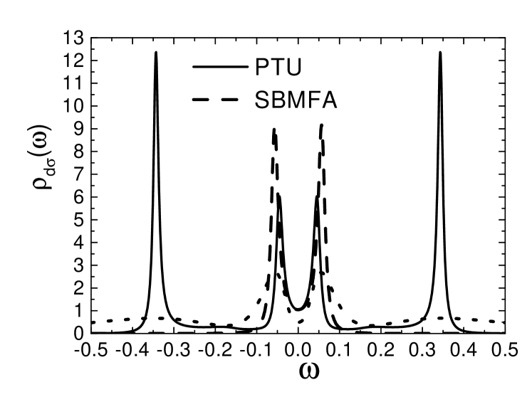
Figure 11: Spectral density of states near the Fermi energy for $U=0.5$, $\Delta_{2}=0.02$ and $\lambda=0.078$. Full line: PTU, dashed line: SBMFA, dotted line: result for $\Delta_{2}=0$ broadened as in NRG calculations (see text)

The results for the spectral density within PTU and SBMFA near the Fermi energy for the smaller two values of $\lambda$ are shown in Fig. 12. For the same reason discussed above, we believe that the splitting and intensity of the peaks for $\lambda=0.0627$ within the SBMFA are exaggerated. As before, the PTU results predict narrower peaks near the Fermi energy than the NRG results. For the smallest value $\lambda=0.0354$, we believe that both, the PTU and the SBMFA including the roots $R_{\sigma}$ and $L_{\sigma}$ exaggerate the width of the only peak near the Fermi energy and the NRG is expected to provide more reliable results. In comparison with the latter, the SBMFA without the roots seems to predict a too narrow Kondo peak. However, even in this case, the NRG is not able to describe properly the narrow side peaks. We expect that this defficency persists as long as $\Delta_{2}<U/2$.

Figure 12: Spectral density of states near the Fermi energy for $U=0.5$, $\Delta_{2}=0.02$ and two values of $\lambda$. Full line: PTU, dashed line: SBMFA.

III.7 Effects of temperature

In Fig. 13 we show the evolution of the spectral density with temperature in a region in which there are split peaks, calculated with the PTU. Similarly to the case of constant $\Delta(\omega)$, the peaks near the Fermi energy decrease in a temperature scale of the order of the half width at half maximum of the structure. In contrast to that case however, some structure remains even at the highest temperatures. This can be understood qualitatively from the behavior observed in the exactly solvable limit $\Delta_{2}=0$.

Figure 13: Spectral density of states near the Fermi level for $\Delta_{2}=0.2\Delta(0)$, $\lambda=\sqrt{\Delta_{2}\Delta(0)}$, $U=4$ and several values of the temperature $T/\Delta(0)$.

In addition, the evolution of the side peaks with temperature is more marked than in the case of constant $\Delta(\omega)$, probably due to the fact that the broadening effects of the temperature are more noticeable when the peaks are narrower.

At temperatures higher than $T=\Delta(0)$, there is little variation in the spectral density. The result for $T=5\Delta(0)$ (not shown) coincides with that for $T=\Delta(0)$ within the width of the line in the figure. It is curious that some structure appears near $\omega/\Delta(0)=\pm 1.2$ at high temperatures. Its origin is unclear to us.

IV Summary and discussion

We have studied an impurity Anderson model in the symmetric case, in which the hybridization function $\Delta(\omega)$ has a Lorentzian shape of width $\Delta_{2}$. The model can be regarded as a simplified version of that proposed to describe the projection of the Kondo effect in quantum corrals (the quantum mirage),rev and is relevant for systems of double QD’s in which one can be regarded as non-interacting and connected to metallic leads (or other system of non-interacting electrons) and the other is interacting and connected as a side dot to the non-interacting one.dias

The characteristic low-energy scale or Kondo temperature $T_{K}$ of the model, changes from the known exponential dependence $T_{K}\simeq D\exp[-\pi U/4\Delta(0)]$ in the Coulomb repulsion $U$ for large $U$ and a flat $\Delta(\omega)$ (large $\Delta_{2}$), to $T_{K}=8\lambda^{2}/U$ for large $U$ and $\Delta_{2}\rightarrow 0$, where $\lambda$ is the interdot hybridization. For small enough $\Delta_{2}\lesssim T_{K}$, the scaling properties of the Kondo regime are lost, but by extension we continue to call “Kondo peak” the structure near the Fermi energy in the spectral density.

When $\Delta_{2}$ becomes smaller than $\sim T_{K}/2$ (see Fig. 8) the characteristic Kondo peak in the spectral density $\rho_{d\sigma}(\omega)$ of the interacting QD near the Fermi energy splits in two. This splitting was reported before in the context of the mirage effect hvar (but not discussed in detail there) and in recent calculations using the numerical renormalization group (NRG).dias Our calculations using perturbation theory in $U$ and a slave-boson mean field approximation (SBMFA) agree qualitatively with these results, but predict narrower split peaks. Moreover, we find that the side peaks of $\rho_{d\sigma}(\omega)$ near the charge transfer energies are much narrower and higher that in the usual case of a flat $\Delta(\omega)$ and than the results presented in Ref. dias, .

In Section III F, we have provided several arguments that indicate that the above mentioned discrepancies are due to shortcomings of the numerical technique. These can be partially overcome if density matrix renormalization group is used in combination with NRG.zit2 Another way of improving the NRG results which has been shown to lead to sharper charge transfer peaks is to calculate the self energy as a ratio of two Green’s functions $\Sigma_{dd\sigma}(z)=U\langle\langle d_{\sigma}d_{\bar{\sigma}}^{\dagger}d_{\bar{\sigma}},d_{\sigma}^{\dagger}\rangle\rangle_{z}/\langle\langle d_{\sigma},d_{\sigma}^{\dagger}\rangle\rangle_{z}$, and replace the result in Eq. (5).bulla This has the advantage that the effect of $\Sigma_{sd\sigma}(z)$ is taken into account exactly.

The splitting of the peaks can be understood qualitatively from the limit $\Delta_{2}\rightarrow 0$, and quantitatively in terms of weakly interacting renormalized quasiparticles, as described in Section III D.

The SBMFA provides an analytical expression, leading to a diagram for the region of parameters for which split peaks in $\rho_{d\sigma}(\omega)$ are expected. This is represented in Fig. 7. In the region in which split peaks are present, some structure remains near the Fermi energy even at temperatures much higher than the Kondo temperature $T_{K}$.

The approximations that we have used satisfy Fermi liquid relations and work well in the limit of small $\Delta_{2}$. In particular the agreement of perturbative calculations with the exact results for $\Delta_{2}\rightarrow 0$ at zero temperature is surprising.

If the non-interacting resonance (the energy of the non-interacting QD) is shifted away from the Fermi energy in some energy larger than its width $\Delta_{2}$, we expect a dramatic change in the spectral density at low energies, with a very narrow Kondo resonance at the Fermi energy, due to the decrease of the non-interacting density of states at the Fermi level, and the exponential dependence of the Kondo energy scale with this density. This is based on previous calculations using approximations rev and supported by NRG results.corna Instead, the side peaks should not be affected substantially.

The presence of narrow side bands in the region in which the Kondo peak splits in two can in principle be tested experimentally in QD systems. The spectral density at the interacting dot can be measured in transport experiments in which another lead is added.leba ; letu

References

- (1) A. C. Hewson, Phys. Rev. Lett. 70, 4007 (1993).
- (2) D. Goldhaber-Gordon, H. Shtrikman, D. Mahalu, D. Abusch-Magder, U. Meirav, and M. A. Kastner, Nature 391, 156 (1998).
- (3) S. M. Cronenwet, T. H. Oosterkamp, and L. P. Kouwenhoven, Science 281, 540 (1998).
- (4) D. Goldhaber-Gordon, J. Göres, M. A. Kastner, H. Shtrikman, D. Mahalu, and U. Meirav, Phys. Rev. Lett. 81, 5225 (1998).
- (5) W. G. van der Wiel, S. de Franceschi, T. Fujisawa, J. M. Elzerman, S. Tarucha, and L. P. Kowenhoven, Science 289, 2105 (2000).
- (6) L.I. Glazman and M.E. Raikh, JETP Lett. 47, 452 (1988).
- (7) T. K. Ng and P. A. Lee, Phys. Rev. Lett. 61, 1768 (1988).
- (8) T. A. Costi, A. C. Hewson, and V. Zlatić, J. Phys. Condens. Matter 6, 2519 (1994).
- (9) H. C. Manoharan, C. P. Lutz, and D. M. Eigler, Nature (London) 403, 512 (2000).
- (10) A. A. Aligia and A. M. Lobos, J. Phys.: Condens. Matter 17, S1095 (2005); references therein.
- (11) A. Lobos and A. A. Aligia, Phys. Rev. B 68, 035411 (2003).
- (12) A. Lobos and A. A. Aligia in Concepts in Electron Correlation, A.C. Hewson and V. Zlatić (eds.) (Kluver Academic Publishers, Netherlands, 2003), p. 229.
- (13) T. Jamneala, V. Madhavan, and M. F. Crommie, Phys. Rev. Lett. 87, 256804 (2001).
- (14) A. A. Aligia, Phys. Rev. Lett. 96, 096804 (2006).
- (15) H. Jeong, A. M. Chang, and M. R. Meloch, Science 304, 565 (2004).
- (16) N. J. Craig, J. M. Taylor, E. A. Lester, C. M. Marcus, M. P. Hanson, and A. C. Gossard, Science 293, 2221 (2001).
- (17) J. C. Chen, A. M. Chang, and M. R. Melloch, Phys. Rev. Lett. 92, 176801 (2004).
- (18) F. R. Waugh, M. J. Berry, D. J. Mar, R. M. Westervelt, K. L. Campman, and A. C. Gossard, Phys. Rev. Lett. 75, 705 (1995).
- (19) L. Gaudreau, S. A. Studenikin, A. S. Sachrajda, P. Zawadzki, A. Kam, J. Lapointe, M. Korkusinski, and P. Hawrylak, Phys. Rev. Lett. 97, 036807 (2006).
- (20) L. P. Kouwenhoven, F. W. J. Hekking, B. J. van Wees, C. J. P. M. Harmans, C. E. Timmering, and C. T. Foxon, Phys. Rev. Lett. 65, 361 (1990).
- (21) Y. Oreg and D. Goldhaber-Gordon, Phys. Rev. Lett. 90, 136602 (2003).
- (22) R. Žitko and J. Bonča, Phys. Rev. B 74, 224411 (2006).
- (23) A. A. Aligia, K. Hallberg, B. Normand, and A. P. Kampf, Phys. Rev. Lett. 93, 076801 (2004).
- (24) G. B. Martins, C. A. Büsser, K. A. Al-Hassanieh, A. Moreo, and E. Dagotto, Phys. Rev. Lett. 94, 026804 (2005).
- (25) P. S. Cornaglia and D. R. Grempel, Phys. Rev. B 71, 075305 (2005).
- (26) R. Žitko and J. Bonča, Phys. Rev. B 73, 035332 (2006).
- (27) A. Oguri , Y. Nisikawa, and A. C. Hewson, J. Phys. Soc. Jpn. 74, 2554 (2005).
- (28) Y. Nisikawa and A. Oguri, Phys. Rev. B 73, 125108 (2006).
- (29) A. M. Lobos and A. A. Aligia, Phys. Rev. B 74, 165417 (2006).
- (30) A. Ramšak, J. Mravlje, R. Žitko and J. Bonča, Phys. Rev. B 74, 241305(R) (2006).
- (31) L. G. G. V. Dias da Silva, N. P. Sandler, K. Ingersent, and S. E. Ulloa, Phys. Rev. Lett. 97, 096603 (2006).
- (32) A. A. Aligia, Phys. Rev. B 64, 121102(R) (2001).
- (33) A. A. Aligia, Phys. Rev. B 66, 165303 (2002).
- (34) G. Chiappe and A. A. Aligia, Phys. Rev. B 66, 075421 (2002); Phys. Rev. B 70, 129903(E) (2004).
- (35) P. S. Cornaglia and C. A. Balseiro, Phys. Rev. B 66, 174404 (2002).
- (36) R. Bulla, A.C. Hewson, and Th. Pruschke, J. Phys. Cond. Matt. 10, 8365 (1998).
- (37) K. Yosida and K. Yamada, Prog. Theor. Phys. Suppl. 46, 244 (1970); Prog. Theor. Phys. 53, 1286 (1975); K. Yamada, ibid 53, 970 (1975).
- (38) B. Horvatić, D. Šokčević, and V. Zlatić, Phys. Rev. B 36, 675 (1987).
- (39) G. Kotliar and A. E. Ruckenstein, Phys. Rev. Lett. 57, 1362 (1986).
- (40) D.C. Langreth, Phys. Rev. 150, 516 (1966).
- (41) A.A. Aligia, Phys. Rev. B 74, 155125 (2006); references therein.
- (42) R. N. Silver, J. E. Gubernatis, D. S. Sivia, and M. Jarrell, Phys. Rev. Lett. 65, 496 (1990).
- (43) A.A. Aligia and C. R. Proetto, Phys. Rev. B 65, 165305 (2002).
- (44) G.D. Mahan, Many Particle Physics (Plenum, New York, 1981).
- (45) M. Abramowitz and I.A. Stegun, Handbook of mathematical functions (Dover, New York, 1965).
- (46) J. M. Luttinger and J. C. Ward, Phys. Rev. 118, 1417 (1960).
- (47) B. Alascio, R. Allub and A. A. Aligia, J. Phys. C 13, 2869 (1980).
- (48) D.E. Logan, M.P. Eastwood, and M.A. Tusch, J. Phys. Cond. Matt. 10, 2673 (1998).
- (49) A. C. Hewson, Phys. Rev. Lett. 70, 4007 (1993).
- (50) E. Lebanon and A. Schiller, Phys. Rev. B 65, 035308 (2001).
- (51) R. Leturcq, L. Schmid, K. Ensslin, Y. Meir, D.C. Driscoll, and A.C. Gossard, Phys. Rev. Lett. 95, 126603 (2005).