Static and dynamic properties of hadronic systems with heavy quarks b and c

Chapter 1 Introduction

Quantum Chromodynamics (QCD) is widely accepted as the theory of the strong interaction. QCD is a gauge theory for the strong interaction of quarks and gluons based on the SU(3) color group. Quarks have been with us since the 60’s when the first three flavors, up ($u$), down ($d$) and strange ($s$), were proposed as members of the fundamental representation for the approximate SU(3) flavor symmetry observed in the hadron spectra. In the simplest picture baryons are made up of three quarks, while most mesons can be explained as made up of a quark and an antiquark. Deep inelastic scattering (DIS) on the proton confirmed this picture of hadrons as bound states of more fundamental particles. The data supported the idea of charged spin-1/2 components or partons inside the nucleon. Those partons were identified with the quarks.

Quarks carry a new quantum number that was named color. The color quantum number can take on three different values and was introduced to solve the statistics problem associated with ground state baryons with three equal quarks. Experimental evidence for the color quantum number comes from the analysis of the $\sigma(e^{+}e^{-}\rightarrow\mathrm{hadrons})/\sigma(e^{+}e^{-}\to\mu^{+}\mu^{-})$ cross sections ratio or the $\pi^{0}\to\gamma\gamma$ decay width. The absence of color will render the theoretical predictions a factor of 3 and 9 respectively below experimental data. Hadrons do not carry the color quantum number, and thus quarks have to combine in such a way that hadrons are “colorless” or color singlets.

Quarks have never been observed as free particles and the consensus is that they are confined in the physical colorless hadrons. While confinement has never been proven in a rigorous way in QCD, there are hints, obtained in Monte Carlo simulations performed in a discretized space-time (see, for example Ref. [1]), that QCD leads to confinement.

In the 70’s ’t Hooft, Politzer [2], Gross and Wilczek [3, 4] found that in nonabelian gauge theories the effective coupling constant decreases at large momentum transfers or short distances while it increases at low momentum transfers or large distances. Both features, called asymptotic freedom and infrared slavery respectively, are necessary to describe quark dynamics. While DIS data, where large momentum transfers are involved, shows the existence of almost free partons inside the nucleon, the absence of free quarks suggests confinement at large distances. Fritzsch and Gell-Mann [5, 6] proposed that quark dynamics was described by a nonabelian gauge theory based on the color quantum number, QCD. The appropriate gauge group was color SU(3). SU(3) has a fundamental representation of dimension 3 that can accommodate the three values for the quark color quantum number. This representation is complex and the antiquark color states belong to the complex conjugate of the fundamental representation. The combination of three quarks or of a quark and an antiquark can give rise to color states which are SU(3) color singlets.

The QCD gauge boson is called gluon. The gluon appears in 8 different color states corresponding to the adjoint representation of color SU(3). Gluons are not observed as free particles and as in the quark case, we think they are bound in the physical hadrons. Evidence for gluons comes from DIS data both from the observation of three jets events, and from the fact that only half of the proton momentum is carried by charged partons. The rest must be attributed to non charged partons, the gluons.

Another important feature of QCD with three quark flavors, and which is essential to understand its low energy spectrum, is chiral symmetry. Chiral symmetry is an approximate symmetry (it is explicitly broken by the quark masses) of the QCD Lagrangian. This symmetry is not shared by the ground state and one talks of a spontaneously broken symmetry. This property manifest itself in the existence of an octet of almost-massless pseudoscalar Goldstone bosons.

With only three quark flavors, the theory of electroweak interactions involving quarks leads to the existence of weak neutral currents with $\Delta S=1$. Those processes were not observed experimentally. The easiest way to avoid this unwanted feature is through the GIM mechanism (from Glashow, Illiopoulos and Maiani [7] ) that required a new quark flavor, the charm ($c$). This new flavor implied the existence of new types of hadrons containing the charm quark or antiquark. The $J/\Psi$ meson discovered in 1974 [9, 10] was interpreted as a bound state of the charm quark and its antiquark. Two years later came the first observation of mesons with open charm [11, 12]. Two more quark flavors, later named bottom ($b$) and top ($t$), were predicted in 1973 by Kobayashi and Maskawa [13] in order to get a realistic model of CP violation in weak theories. The discovery of the $\tau$ lepton in 1974-1977 led further theoretical support to the existence of the bottom and top quarks as the cancellation of the triangle anomaly in the electroweak theory required as many quarks as there were leptons (also that the former appeared in three colors). The $\Upsilon$ meson discovered in 1977 [14] was interpreted as being a $b\bar{b}$ state. Top discovery had to await for another 17 years when it was finally seen in proton-antiproton collisions [15].

In the large energy regime QCD can be treated perturbatively and predictions of the theory have shown a remarkable agreement with experiment. On the other hand at low energies QCD becomes nonperturbative and it is not known how to solve it exactly. In this low energy regime there are approaches which make approximations to the exact solutions like QCD sum rules and Lattice QCD.

Another approach to QCD in the low energy regime is the use of phenomenological models which are not directly derived from QCD but include some of its basic properties. Constituent quark models (CQM) are among these. In CQM models hadrons are simply modeled, as bound states of three valence quarks (baryons) or a quark and an antiquark (mesons). Those quarks are quasiparticle degrees of freedom with the same quantum numbers as QCD quarks, differing from the latter in their masses and in the fact that they could have an internal structure.

Among CQM, nonrelativistic quark models (NRQM) have shown to be phenomenologically very successful. In these models constituent quarks are treated nonrelativistically and they interact through potentials that mimic QCD asymptotic freedom and confinement. In fact it was this simple nonrelativistic picture that led to the necessity for the color quantum number. The vast literature on NRQM calculations forbids to quote here but a few works. An early success of NRQM calculations was the satisfactory account of the magnetic moments of the octet baryons [16]. Baryon spectra was studied within the NRQM by Isgur and Karl in a series of papers [17, 18, 19, 20, 21, 22] where it was shown that a model with nonrelativistic point-like quarks moving in a flavor independent confining potential, perturbed by color hyperfine interactions, was able to explain the main features of the spectra. Meson spectra was equally well described within the NRQM [23]. Color hyperfine interactions among quarks are generated through the one gluon exchange potential first introduced in [8]. The spin-spin part of this potential explains in a simple way the difference in mass between octet and decuplet baryons and between pseudoscalar and vector mesons. The NRQM was extended to the two nucleon system in the 80’s being able to explain, in a more fundamental picture, the short range nucleon-nucleon repulsion in S-wave scattering as due to one gluon exchange between quarks with a simultaneous quark exchange between the two three-quark clusters [24, 25, 26]. Chiral symmetry and its spontaneously breaking was also incorporated into the NRQM [27] and inter-quark potentials coming from one-Goldstone boson exchanges naturally appeared [28, 29, 30]. In a linear realization of chiral symmetry with two quark flavors not only the Golstone bosons (pions) but also their chiral partner (sigma) was considered. The inclusion of the latter improved the theoretical prediction of $NN$ phase shifts [31, 32] and deuteron properties [33]. Some authors advocated that the one-gluon exchange part of the potential be discarded altogether in favor of only Goldstone boson exchanges [34]. This exclusive view had big problems and was heavily critizied [35]. Most versions of the NRQM use a mixture of both one-gluon and one-Golstone boson exchanges. More recently the study of dibaryons [36, 37, 38], tribaryons [38, 39] and tetraquarks [40, 41, 42] systems have also been addressed in the NRQM. For a recent review on few baryon systems studies see [43]. Electromagnetic [44, 45, 46, 47, 48, 49, 50, 51] and weak [52, 53, 54, 55, 56] form factors have also been analyzed in the NRQM and exchange current contributions to these observables have been studied with detail [46, 47, 48, 49, 50, 54, 56].

In this thesis our interest is in the analysis, within the framework of a NRQM, of static and dynamic properties, the latter related to weak decays, of hadrons with one and two heavy quarks $c$ and/or $b$. In systems with a heavy quark with mass much larger than the QCD scale ($\Lambda_{QCD}$) a new symmetry known as heavy quark symmetry (HQS) arises [57, 58, 59, 60, 61, 62]. HQS is an approximate SU($N_{F}$) symmetry of QCD, being $N_{F}$ the number of heavy flavors ($c$, $b$,…), that appears in systems containing heavy quarks with masses much larger than the typical quantities ($\Lambda_{QCD},m_{u},m_{d},m_{s},\dots)$ which set up the energy scale of the dynamics of the remaining degrees of freedom. In that limit the dynamics of the light quark degrees of freedom becomes independent of the heavy quark flavor and spin. This is similar to what happens in atomic physics where the electron properties are approximately independent of the spin and mass of the nucleus (for a fixed nuclear charge). HQS can be cast into the language of an effective theory (HQET)[63] that allows a systematic, order by order, evaluation of corrections to the infinite mass limit in inverse powers of the heavy quark masses. HQS and HQET have proved very useful tools to understand bottom and charm physics and they have been extensively used to describe the dynamics of systems containing a heavy $c$ or $b$ quark [64, 65]. For instance, all lattice QCD simulations rely on HQS to describe bottom systems [66, 67, 68, 69, 70]. In the case of systems with two heavy quarks one can not directly apply HQS. It is known that the kinetic energy term, needed in those systems to regulate infrared divergences, breaks heavy flavor symmetry [71]. Still, there is a symmetry that survives: heavy quark spin symmetry (HQSS) [72]. This symmetry amounts to the decoupling of the two heavy quark spins since the spin–spin interaction vanishes for infinite heavy quark masses.

The constraints imposed by HQS and HQSS have not been systematically employed in the context of nonrelativistic quark models. We intend to study hadrons with one and two heavy $c$ and/or $b$ quarks in a NRQM making full use of those constraints. For instance, those constraints will simplify notably the resolution of the three-body problem in baryons allowing for the use of a simple variational ansatz. A NRQM treatment of those systems will comply with the model independent predictions of HQS and HQSS in the infinite heavy quark mass limit, as in that limit all spin-spin interactions terms involving heavy quarks vanish. Another question is to what extend the deviations from the infinite heavy quark mass limit in a NRQM calculation agree with the predictions of HQET.

This thesis is organized as follows. In chapter 2 we briefly introduce the quark-quark potentials that have been used throughout this work.

In chapter 3 we study leptonic decays of pseudoscalars $B,\,D$ and vector $B^{*},\,D^{*}$ mesons, and $B\to D$ and $B\to D^{*}$ semileptonic decays. In the latter case full form factors are computed and used to get differential and total decay widths. When possible these form factors are improved using corrections from HQET. We make a prediction for the value of the $|V_{cb}|$ Cabbibo-Kobayashi-Maskawa (CKM) matrix element which compares well with experimental determinations.
Also in this chapter we will use partial conservation of the axial current (PCAC) to relate axial current matrix elements with the pion emission amplitude and in this way make a prediction for the strong coupling constants $g_{BB^{*}\pi}$ and $g_{DD^{*}\pi}$.

Exclusive semileptonic and nonleptonic two-meson decays of the $B_{c}^{-}$ meson have been analyzed in chapter 4, where a fairly exhaustive study of these decays is done. In semileptonic decays we have excluded processes that involve a $b\to u$ transition at the quark level where the NRQM fails due to the large recoil momenta and the ignorance of resonance exchanges. Similarly in nonleptonic two-meson decays we shall only consider channels with at least a $c\bar{c}$ or $B$ final meson.

In chapter 5 we study baryons with two heavy quarks. A procedure to solve the three-body problem in an approximate way using a variational ansatz is presented. We obtain the spectrum and wave functions that are further used to compute different static properties. The infinite heavy quark mass limit of the wave functions is studied and as expected they comply with HQSS model independent predictions.

In chapter 6 we use the wave functions computed in the previous chapter to study semileptonic decays of doubly heavy baryons. Full form factors, decay widths, and angular asymmetries are studied.

Finally chapter 7 is devoted to the study of the strong one pion decay of baryons with a heavy quark. As in chapter 3 PCAC is used to relate weak axial current matrix elements with the pion emission amplitude.

Chapter 2 Quark quark potentials used in this work

2.1 Introduction

In this chapter we give a brief account of the quark-quark potentials that we use in this work to get the hadron wave functions. We shall use five different two-body phenomenological potentials. One of these potentials (BHAD) has been taken from Ref. [73] and four others (AL1, AL2, AP1, AP2) from Refs. [74, 75]. The use of different potentials will allow us to check the sensitivity of our results to the inter-quark interaction.

All these potentials share a common structure that includes a confining term plus Coulomb and hyperfine terms coming from the one-gluon exchange potential. They differ in the form factor used in the hyperfine and $1/r$ terms and/or in the power chosen for the confining term. All of them neglect the tensor and spin-orbit pieces also present in the one-gluon exchange potential [8] on the account that they are not essential to describe the global features of hadron spectroscopy. As a consequence both the total orbital angular momentum $L$ and the total spin $S$ are separately good quantum numbers. Chiral symmetry is not incorporated in these potentials and thus no terms generated by Goldstone boson exchange are included. Explicit expressions appear in what follows.

2.2 BHAD, AL1, AL2, AP1 and AP2 potentials

For the $q\overline{q}$ case they can be given in the general form

$$V_{ij}^{q\bar{q}}(r)= -\frac{\kappa\left(1-e^{-r/r_{c}}\right)}{r}+\lambda r^{p}-\Lambda$$ (2.1)

$$+\left\{a_{0}\frac{\kappa}{m_{i}m_{j}}\frac{e^{-r/r_{0}}}{rr_{0}^{2}}+\frac{2\pi}{3m_{i}m_{j}}\kappa^{\prime}\left(1-e^{-r/r_{c}}\right)\frac{e^{-r^{2}/x_{0}^{2}}}{\pi^{\frac{3}{2}}x_{0}^{3}}\right\}\vec{\sigma}_{i}\vec{\sigma}_{j}$$

where $i,j=(l(u.d),s,c,b)$, $\vec{\sigma}$ are the spin Pauli matrices, $m_{i}$ the quark masses and

$$x_{0}(m_{i},m_{j})=A\left(\frac{2m_{i}m_{j}}{m_{i}+m_{j}}\right)^{-B}$$ (2.2)

Parameters for the different potentials are summarized in Table 2.1.

	BHAD	AL1	AL2	AP1	AP2
$\kappa$	0.52	0.5069	0.5871	0.4242	0.5743
$r_{c}$[GeV-1]	0.	0.	0.1844	0.	0.3466
$p$	1	1	1	2/3	2/3
$\lambda$ [GeV(1+p)]	0.186	0.1653	0.1673	0.3898	0.3978
$\Lambda$ [GeV]	0.9135	0.8321	0.8182	1.1313	1.1146
$a_{0}$	1	0	0	0	0
$r_{0}$ [GeV-1]	2.305	—	—	—	—
$\kappa^{\prime}$	0.	1.8609	1.8475	1.8025	1.8993
$m_{u}=m_{d}$ [GeV]	0.337	0.315	0.320	0.277	0.280
$m_{s}$ [GeV]	0.600	0.577	0.587	0.553	0.569
$m_{c}$ [GeV]	1.870	1.836	1.851	1.819	1.840
$m_{b}$ [GeV]	5.259	5.227	5.231	5.206	5.213
$B$	—	0.2204	0.2132	0.3263	0.3478
$A$ [GeVB-1]	—	1.6553	1.6560	1.5296	1.5321

Table 2.1: Parameters for the BHAD, AL1, AL2, AP1 and AP2 potentials taken from Refs. [73, 75]

Note that the $a_{0}$ and $\kappa^{\prime}$ terms are mutually exclusive. The power $p$ chosen for the confining term is $p=1$ for the BHAD, AL1, AL2 potentials. This linear confinement is suggested by lattice results [76]. The AP1 and AP2 potentials use instead $p=\frac{2}{3}$ which is needed, in a nonrelativistic approach, to get the correct asymptotic Regge trajectories for large angular momentum mesons [77]. The hyperfine term comes from the one-gluon exchange potential and the original $\delta(\vec{r})$ dependence has been smeared out in order that nonperturbative calculations are possible. The BHAD potential uses a Yukawa form factor, while AL1, AL2, AP1 and AP2 potentials use a gaussian form factor. In these latter cases the depth and width of the gaussian depends on the constituent quark masses allowing for a better reproduction of the hyperfine splitting of heavy mesons. The phenomenological formula in Eq. (2.2), originally proposed in [78], seems to be well suited for that purpose [79]. The AL2 and AP2 potentials include a further form factor in the $1/r$ and hyperfine terms with a shape given by $(1-\exp(-r/r_{c}))$. This factor simulates asymptotic freedom and its inclusion seems to be more important for heavy mesons than for light ones. Finally note that the $\kappa$ and $\kappa^{\prime}$ parameters in the AL1, AL2, AP1 and AP2 potentials would be the same if one simply replaced the original $\delta(\vec{r})$ function in the hyperfine term by the gaussian form factor. The fact that they are different allows for a great improvement in the results [79]. This is also true for the BHAD potential where the strength for the hyperfine term, where the $\delta(\vec{r})$ function has been replaced by a Yukawa form factor, is six times larger than the one used in the $1/r$ term. This, in effect, is allowing for sources of hyperfine interaction other than the one-gluon exchange.

All free parameters in the potentials were adjusted in the original works to reproduce the light and heavy-light meson spectra (AL1,AL2,AP1,AP2), or to fit the low-lying levels of charmonium (BHAD). In this latter case $m_{b}$ and $m_{s}$ were adjusted to reproduce the ground state of the $\Upsilon$ and $\phi$ mesons respectively while the light quark mass $m_{l}$ was chosen from magnetic moments considerations.

To obtain the quark-quark potential we shall use, as has been done in Refs. [73, 74, 75], the prescription

$$V_{ij}^{qq} = \frac{V_{ij}^{q\bar{q}}}{2}$$ (2.3)

This relation assumes the potential has a global color dependence given by $\vec{\lambda}^{c}_{i}\vec{\lambda}^{c}_{j}$ , where $\vec{\lambda}^{c}$ stands for the Gell-Mann matrices in the color space.

Chapter 3 Leptonic and semileptonic decays of mesons with a heavy quark

3.1 Introduction

This chapter is devoted to the calculation of different weak observables of pseudoscalar and vector mesons with a heavy quark. These weak observables are of great interest since they help to probe the quark structure of the involved hadrons, and also provide information to determinate the absolute value of elements of the CKM matrix.

In Ref. [80], in which a similar model was used to study the $\Lambda_{b}^{0}\to\Lambda^{+}_{c}\,l^{-}\bar{\nu}_{l}$ and $\Xi_{b}^{0}\to\Xi^{+}_{c}\,l^{-}\bar{\nu}_{l}$ reactions, it was shown that a direct nonrelativistic calculation does not meet HQET constraints. This problem was solved imposing HQET relations among form factors. That led to a determination of the $|V_{cb}|$ CKM matrix element in good agreement with experimental results.

One would expect this problem will also show up in this calculation, so that constraints coming from HQET will be included at some point in the calculation in order to improve the results.

In the case of mesons with a heavy quark, HQS leads to many model independent predictions. For instance in the HQS limit the masses of the lowest lying (s-wave) pseudoscalar and vector mesons with a heavy quark are degenerate. Nonrelativistic quark models satisfy this constraint: the spin-spin terms, that distinguishes vector from pseudoscalar, are zero if the mass of the heavy quark goes to infinity. HQS also predicts that the masses and leptonic decay constants of pseudoscalars and vector mesons are related via

$$f_{P}\,m_{P}\Bigg{|}_{HQS}=f_{V}\,m_{V}\Bigg{|}_{HQS}$$ (3.1)

relation that is also satisfied in the quark model in the HQS limit. If one looks now at the form factors for the semileptonic $B\to D$ and $B\to D^{*}$ decays HQS predicts relations among different form factors that are also met by the quark model in the HQS limit. The question is to what extent the deviations from the HQS limit evaluated in the quark model agree with the constraints deduced from HQET. In addition we will make use of these HQET constraints to improve the quark model results and thus come up with reliable predictions.

Apart from lattice QCD and QCD sum rules (QCDSR) calculations with which we shall compare our results, and that will be quoted in the following, the different observables analyzed in this work have been studied in the quark model starting with the pioneering work of Ref. [81, 82, 83] within a non relativistic version, to continue with different versions of the relativistic quark model applied to the determination of decay constants [84, 85, 86, 87, 88, 89, 90, 91, 92, 93], form factors and differential decay widths [91, 93, 94, 95, 96, 97, 98, 99, 100, 101, 102], Isgur-Wise functions [93, 103, 104, 105, 106, 107, 108, 109, 110] or strong coupling constants [91, 108, 111, 112, 113, 114].

For calculations in this chapter we have used experimental meson masses taken from Ref. [115].

3.2 Meson states

For a meson $M$ we use the following expression for the wave function in the Fock-space representation.

$$\left|{M,\lambda\,\vec{P}}\,\right\rangle_{NR}\,=\,\int d^{3}p\sum_{\alpha_{1},\alpha_{2}}\hat{\phi}^{(M,\lambda)}_{\alpha_{1},\alpha_{2}}(\,\vec{p}\,)$$

$$\frac{(-1)^{\frac{1}{2}-s_{2}}}{(2\pi)^{\frac{3}{2}}\sqrt{2E_{f_{1}}(\vec{p}_{1})2E_{f_{2}}(\vec{p}_{2})}}\ \left|\ q,\ \alpha_{1}\ \vec{p}_{1}=\frac{m_{f_{1}}}{m_{f_{1}}+m_{f_{2}}}\vec{P}-\vec{p}\ \right\rangle$$

$$\hskip 133.72786pt\left|\ \bar{q},\ \alpha_{2}\ \vec{p}_{2}=\frac{m_{f_{2}}}{m_{f_{1}}+m_{f_{2}}}\vec{P}+\vec{p}\ \right\rangle$$ (3.2)

where $\vec{P}$ stands for the meson three momentum and $\lambda$ represents the spin projection in the meson center of mass. $\alpha_{1}$ and $\alpha_{2}$ represent the quantum numbers of spin (s), flavor (f) and color (c)

$$\alpha\equiv(s,f,c)$$ (3.3)

of the quark and the antiquark, while $E_{f_{1}}(\vec{p}_{1}),\,\vec{p}_{1}$ and $E_{f_{2}}(\vec{p}_{2}),\,\vec{p}_{2}$ are their respective energies and three-momenta. $m_{f}$ is the mass of the quark or antiquark with flavor $f$. The factor $(-1)^{\frac{1}{2}-s_{2}}$ is included in order that the antiquark spin states have the correct relative phase. The normalization of the quark and antiquark states is

$$\left\langle\ \alpha^{\prime}\ \vec{p}^{\ \prime}\,|\,\alpha\ \vec{p}\,\right\rangle=\delta_{\alpha^{\prime},\ \alpha}\,(2\pi)^{3}\,2E_{f}(\vec{p})\,\delta(\vec{p}^{\ \prime}-\vec{p}\,)$$ (3.4)

Furthermore, $\hat{\phi}^{\,(M,\lambda)}_{\alpha_{1},\alpha_{2}}(\,\vec{p}\,)$ is the momentum space wave function for the relative motion of the quark-antiquark system. Its normalization is given by

$$\int\,d^{3}p\ \sum_{\alpha_{1}\,\alpha_{2}}\left(\hat{\phi}^{\,(M,\lambda^{\prime})}_{\alpha_{1},\,\alpha_{2}}(\,\vec{p}\,)\right)^{*}\hat{\phi}^{\,(M,\lambda)}_{\alpha_{1},\,\alpha_{2}}(\,\vec{p}\,)=\delta_{\lambda^{\prime},\,\lambda}$$ (3.5)

and, thus, the normalization of our meson states is

$${}_{\stackrel{{\scriptstyle}}{{NR}}}\left\langle\,{M,\lambda^{\prime}\,\vec{P}^{\,\prime}}\,|\,{M,\lambda\,\vec{P}}\,\right\rangle_{NR}=\delta_{\lambda^{\prime},\,\lambda}\,(2\pi)^{3}\,\delta(\vec{P}^{\,\prime}-\vec{P}\,)$$ (3.6)

For the particular case of ground state pseudoscalar ($P$) and vector ($V$) mesons we can assume the orbital angular momentum to be zero and then we will have

$$\hat{\phi}^{\,(P)}_{\alpha_{1},\,\alpha_{2}}(\,\vec{p}\,) = \frac{1}{\sqrt{3}}\,\delta_{c_{1},\,c_{2}}\ \hat{\phi}^{\,(P)}_{(s_{1},\,f_{1}),\,(s_{2},\,f_{2})}(\,\vec{p}\,)$$

$$= \frac{1}{\sqrt{3}}\,\delta_{c_{1},\,c_{2}}\ (-i)\ \hat{\phi}^{\,(P)}_{f_{1},\,f_{2}}(\,|\vec{p}\,|)\ Y_{00}(\,\widehat{\vec{p}}\ )\ \left(\left.\frac{1}{2},\frac{1}{2},0\right|s_{1},s_{2},0\right)$$

$$\hat{\phi}^{\,(V,\,\lambda)}_{\alpha_{1},\,\alpha_{2}}(\,\vec{p}\,) = \frac{1}{\sqrt{3}}\,\delta_{c_{1},\,c_{2}}\ \hat{\phi}^{\,(V,\,\lambda)}_{(s_{1},\,f_{1}),\,(s_{2},\,f_{2})}(\,\vec{p}\,)$$ (3.7)

$$= \frac{1}{\sqrt{3}}\,\delta_{c_{1},\,c_{2}}\ (-1)\ \hat{\phi}^{\,(V)}_{f_{1},\,f_{2}}(\,|\vec{p}\,|)\ Y_{00}(\,\widehat{\vec{p}}\ )\ \left(\left.\frac{1}{2},\frac{1}{2},1\right|s_{1},s_{2},\lambda\right)$$

where $(j_{1},j_{2},j_{3}|m_{1},m_{2},m_{3})$ is a Clebsch-Gordan coefficient, $Y_{00}=1/\sqrt{4\pi}$ is the $l=m=0$ spherical harmonic, and $\hat{\phi}^{\,(M)}_{f_{1},\,f_{2}}(|\,\vec{p}\,|)$ is the Fourier transform of the radial coordinate space wave function. The phases are introduced for later convenience.

To evaluate the coordinate space wave function we shall use the potentials presented in chapter 2. This will provide us with a spread of results that we will consider, and quote, as a theoretical error to the averaged value that we will quote as our central result. Another source of theoretical uncertainty, that we can not account for, is the use of nonrelativistic kinematics in the evaluation of the orbital wave functions and the construction of our states defined above. While this is a very good approximation for mesons with two heavy quarks (as the $B_{c}$ that will be studied in chapter 4), it is not that good for mesons with a light quark. That notwithstanding note that any nonrelativistic quark model has free parameters in the inter-quark interaction that are fitted to experimental data. In that sense we think that at least part of the ignored relativistic effects are included in an effective way in their fitted values.

3.3 Leptonic decay of pseudoscalar and vector $B$ and $D$ mesons

In this section we will consider the purely leptonic decay of pseudoscalars ($B$, $D$) and vector ($B^{*}$, $D^{*}$) mesons. The charged weak current operator for a specific pair of quark flavors $f_{1}$ and $f_{2}$ reads

$$J^{f_{1}\,f_{2}}_{\mu}(0)=J^{f_{1}\,f_{2}}_{V\,\mu}(0)-J^{f_{1}\,f_{2}}_{A\,\mu}(0)=\sum_{(c_{1},\,s_{1}),\,(c_{2},\,s_{2})}\,\delta_{c_{1},\,c_{2}}\ \overline{\Psi}_{\alpha_{1}}(0)\gamma_{\mu}(1-\gamma_{5})\Psi_{\alpha_{2}}(0)$$ (3.8)

with $\Psi_{\alpha_{1}}$ a quark field of a definite spin, flavor and color. The hadronic matrix elements involved in the processes can be parametrized in terms of a unique pseudoscalar $f_{P}$ or vector $f_{V}$ decay constant as

$$\left\langle 0\right|\,J_{\mu}^{f_{1}\,f_{2}}(0)\,\left|\,P,\vec{P}\,\right\rangle=\left\langle 0\right|\,-J_{A\,\mu}^{f_{1}\,f_{2}}(0)\,\left|\,P,\vec{P}\,\right\rangle=-iP_{\mu}\,f_{P}$$

$$\left\langle 0\right|\,J_{\mu}^{f_{1}\,f_{2}}(0)\,\left|\,V,\lambda\,\vec{P}\,\right\rangle=\left\langle 0\right|\,J_{V\,\mu}^{f_{1}\,f_{2}}(0)\,\left|\,V,\,\lambda\,\vec{P}\,\right\rangle=\varepsilon_{(\lambda)\mu}(\,\vec{P}\,)m_{V}f_{V}$$ (3.9)

where the meson states are normalized such that

$$\left\langle\,{M,\lambda^{\prime}\,\vec{P}^{\,\prime}}\,|\,{M,\lambda\,\vec{P}}\,\right\rangle=\delta_{\lambda^{\prime},\,\lambda}\,(2\pi)^{3}\,2E_{M}(\vec{P})\,\delta(\vec{P}^{\,\prime}-\vec{P}\,)$$ (3.10)

with $E_{M}(\vec{P})$ the energy of the meson.

In the first of Eqs.(3.3) $P_{\mu}$ is the four-momentum of the meson, while in the second $m_{V}$ and $\varepsilon_{(\lambda)}(\,\vec{P}\,)$ are the mass and the polarization vector of the vector meson. In both cases $f_{1}$ and $f_{2}$ are the flavors of the quark and the antiquark that make up the meson. Expressions for the different polarization vectors used in this memory are presented in appendix A.

Concerns about the experimental determination of the pseudoscalars decay constants have been raised in Ref. [116]. There the effect of radiative decays was analyzed concluding that for $B$ mesons the decay constant determination could be greatly affected by radiative corrections. In the vector sector, and as rightly pointed out in Ref. [117], the vector decay constants are not relevant from a phenomenological point of view since $B^{*}$ and $D^{*}$ will decay through the electromagnetic and/or strong interaction. They are nevertheless interesting as a mean to test HQS relations.

For mesons at rest we will obtain

$$f_{P}=\frac{-i}{m_{P}}\,\left\langle 0\right|\,J_{A\,0}^{f_{1}\,f_{2}}(0)\,\left|\,P,\vec{0}\,\right\rangle$$

$$f_{V}=\frac{-1}{m_{V}}\,\left\langle 0\right|\,J_{V\,3}^{f_{1}\,f_{2}}(0)\,\left|\,V,\,0\,\vec{0}\,\right\rangle$$ (3.11)

with $m_{P}$ the mass of the pseudoscalar meson. In our model, and due to the different normalization of our meson states, we shall evaluate the decay constants as

$$f_{P}=-i\,\sqrt{\frac{2}{m_{P}}}\,\left\langle 0\right|\,J_{A\,0}^{f_{1}\,f_{2}}(0)\,\left|\,P,\vec{0}\,\right\rangle_{NR}$$

$$f_{V}=-\sqrt{\frac{2}{m_{V}}}\,\left\langle 0\right|\,J_{V\,3}^{f_{1}\,f_{2}}(0)\,\left|\,V,\,0\,\vec{0}\,\right\rangle_{NR}$$ (3.12)

The corresponding matrix elements are given in appendix B.

The results that we obtain for the different decay constants appear in Tables 3.1 and  3.2. Starting with $f_{D}$ and $f_{D_{s}}$ our results are larger that the ones obtained in the lattice by the UKQCD Collaboration [118] or the ones evaluated using QCD spectral sum rules (QSSR) [119, 120]. Not only the independent values are larger but also the ratio $f_{D_{s}}/f_{D}$ is larger in our case. On the other hand our results are in better agreement with other lattice determinations [121, 122]. They also compare very well with the experimental measurements of $f_{D}$ and $f_{D_{s}}$ in Refs. [123, 124, 125, 126, 127, 128]. As for $f_{B}$ and $f_{B_{s}}$, we find a very good agreement in the case of $f_{B_{s}}$ between our results and the ones obtained in the lattice or with the use of QSSR. For $f_{B}$ our result is smaller and then also our ratio $f_{B_{s}}/f_{B}$ is larger.

	$f_{D}$ [MeV]	$f_{D_{s}}$ [MeV]	$f_{D_{s}}/f_{D}$
This work	$243^{+21}_{-17}$	$341^{+7}_{-5}$	$1.41^{+0.08}_{-0.09}$
Experimental data
CLEO	$222.6\pm 16.7^{+2.8}_{-3.4}$ [123]	$280\pm 19\pm 28\pm 34$ [124]	—
ALEPH [125]	—	$285\pm 19\pm 40$	—
OPAL [126]	—	$286\pm 44\pm 41$	—
BEATRICE [127]	—	$323\pm 44\pm 12\pm 34$	—
E653 [129]	—	$194\pm 35\pm 20\pm 14$	—
BES [128]	$371^{+129}_{-119}\pm 25$	—	—
Lattice data
UKQCD [118]	$206(4)^{+17}_{-10}$	$229(3)^{+23}_{-12}$	$1.11(1)^{+1}_{-1}$
Fermilab Lattice [121]	$201\pm 3\pm 6\pm 9\pm 13$	$249\pm 3\pm 7\pm 11\pm 10$	—
M. Wingate et al. [122]	—	$290\pm 20\pm 29\pm 29\pm 6$	—
QCD Spectral Sum Rules
S. Narison: [119, 120]	$203\pm 23$	$235\pm 24$	$1.15\pm 0.04$
	$f_{B}$ [MeV]	$f_{B_{s}}$ [MeV]	$f_{B_{s}}/f_{B}$
This work	$155^{+15}_{-12}$	$239^{+9}_{-7}$	$1.54^{+0.09}_{-0.08}$
Experimental data
BELLE [130]	$229^{+36}_{-31}\,{}^{+34}_{-37}$	—	—
Lattice data
UKQCD [118]	$195(6)^{+24}_{-23}$	$220(6)^{+23}_{-18}$	$1.13(1)^{+1}_{-1}$
M. Wingate et al. [122]	—	$260\pm 7\pm 26\pm 8\pm 5$	—
Lattice world averages	$200\pm 30$ [131]	$230\pm 30$  [132]	$1.16\pm 0.04$ [131]
QCD Spectral Sum Rules
S. Narison [119, 120]	$207\pm 21$	$240\pm 24$	$1.16\pm 0.04$

Table 3.1: Pseudoscalar $f_{P}$ decay constants for $B$ and $D$ mesons

	$\tilde{f}_{D^{*}}$	$\tilde{f}_{D^{*}_{s}}$	$\tilde{f}_{D^{*}}/\tilde{f}_{D^{*}_{s}}$
This work	$9.1^{+0.9}_{-0.9}$	$6.5^{+0.3}_{-0.4}$	$1.41^{+0.06}_{-0.05}$
UKQCD [118]	$8.6(3)^{+5}_{-9}$	$8.3(2)^{+5}_{-5}$	$1.04(1)^{+2}_{-2}$
	$\tilde{f}_{B^{*}}$ [MeV]	$\tilde{f}_{B^{*}_{s}}$ [MeV]	$\tilde{f}_{B^{*}}/\tilde{f}_{B^{*}_{s}}$
This work	$35.6^{+3.4}_{-3.4}$	$23.0^{+1.0}_{-1.5}$	$1.55^{+0.07}_{-0.06}$
UKQCD [118]	$28(1)^{+3}_{-4}$	$25(1)^{+2}_{-3}$	$1.10(2)^{+2}_{-2}$

Table 3.2: $\tilde{f}_{V}=m_{V}/f_{V}$ for $B^{*}$ and $D^{*}$ mesons

For the vector meson decay constants we obtain the values

$$f_{D^{*}}=223^{+23}_{-19}\,{\mathrm{M}eV}\hskip 28.45274ptf_{D_{s}^{*}}=326^{+21}_{-17}\,{\mathrm{M}eV}$$

$$f_{B^{*}}=151^{+15}_{-13}\,{\mathrm{M}eV}\hskip 28.45274ptf_{B_{s}^{*}}=236^{+14}_{-11}\,{\mathrm{M}eV}$$ (3.13)

which are very much the same as the values obtained for the decay constants of their pseudoscalar counterparts. This almost equality of pseudoscalar and vector decay constants is expected in HQS in the limit where the heavy quark masses go to infinity where one would have [61, 62]

$$f_{V}\,m_{V}=f_{P}\,m_{P}\hskip 28.45274pt,\hskip 28.45274ptm_{V}=m_{P}$$ (3.14)

Our decay constants satisfy the above relation within 2%. On the other hand UKQCD lattice data show deviations as large as 20% for D mesons [118].

In order to compare the values of the vector decay constants with lattice data from Ref. [118] we give in Table 3.2 the quantity $\tilde{f}_{V}=m_{V}/f_{V}$. We find good agreement for $\tilde{f}_{D^{*}}$ and $\tilde{f}_{B_{s}^{*}}$ but not so much for the other two. Also our ratios $\tilde{f}_{D^{*}}/\tilde{f}_{D_{s}^{*}}$ and $\tilde{f}_{B^{*}}/\tilde{f}_{B_{s}^{*}}$ are larger than the ones favored by lattice calculations.

On the other hand the ratio

$$\frac{f_{B^{*}}\sqrt{m_{B}}}{f_{D^{*}}\sqrt{m_{D}}}=1.138^{+0.011}_{-0.008}$$ (3.15)

is in very good agreement with the expectation in Ref. [133] where they would get $1.05\sim 1.20$ for that ratio.

3.4 Semileptonic decay of $B$ into $Dl\bar{\nu}$ and $D^{*}l\bar{\nu}$

In this case the hadronic matrix elements are parametrized as

$$\frac{\left\langle\,D,\,\vec{P}^{\prime}\,\left|\,J^{c\,b}_{\mu}(0)\,\right|\,B,\,\vec{P}\right\rangle}{\sqrt{m_{B}m_{D}}} = \frac{\left\langle\,D,\,\vec{P}^{\prime}\,\left|\,J^{c\,b}_{V\,\mu}(0)\,\right|\,B,\,\vec{P}\right\rangle}{\sqrt{m_{B}m_{D}}}$$ (3.16)

$$= \left(v+v^{\prime}\right)_{\mu}\,h_{+}(w)+\left(v-v^{\prime}\right)_{\mu}\,h_{-}(w)$$

$$\frac{\left\langle\,D^{*},\,\lambda\,\vec{P}^{\prime}\,\left|\,J^{c\,b}_{\mu}(0)\,\right|\,B,\,\vec{P}\right\rangle}{\sqrt{m_{B}m_{D^{*}}}} = -\varepsilon_{\mu\nu\alpha\beta}\,\left(\varepsilon_{(\lambda)}^{\nu}(\,\vec{P}^{\prime}\,)\right)^{*}\,v^{\alpha}\,v^{\prime\,\beta}\,h_{V}(w)$$

$$-\,i\,\left(\varepsilon_{(\lambda)\mu}(\,\vec{P}^{\prime}\,)\right)^{*}\,(w+1)\,h_{A_{1}}(w)$$

$$+\,i\,\left(\varepsilon_{(\lambda)\,}(\,\vec{P}^{\prime}\,)\right)^{*}\cdot v\,\left(v_{\mu}\,h_{A_{2}}(w)+v^{\prime}_{\mu}\,h_{A_{3}}(w)\right)$$

where $v=P/m_{B}$ and $v^{\prime}=P^{\prime}/m_{D,\,D^{*}}$ are the four velocities of the initial $B$ and final $D,\,D^{*}$ mesons, $w=v\cdot v^{\prime}\,$ and $\varepsilon_{\mu\nu\alpha\beta}$ is the fully antisymmetric tensor with $\varepsilon^{0123}=+1$.

In the limit of infinite heavy quark masses $m_{c},\,m_{b}\to\infty$ HQS reduces the six form factors to a unique universal function $\xi(w)$ known as the Isgur-Wise function [61, 62]

$$h_{+}(w)=h_{A_{1}}(w)=h_{A_{3}}(w)=h_{V}(w)=\xi(w)$$ (3.19)

$$h_{-}(w)=h_{A_{2}}(w)=0$$ (3.20)

Vector current conservation in the equal mass case implies the normalization

$$\xi(1)=1$$ (3.21)

Away from the heavy quark limit those relations are modified by QCD corrections so that one has

$$h_{j}(w)=\left(\alpha_{j}+\beta_{j}(w)+\gamma_{j}(w)+{\cal O}(1/m_{c,b}^{2})\right)\,\xi(w)$$ (3.22)

The $\alpha_{j}$ are constants fixed by the behavior of the form factor in the heavy quark limit

$$\alpha_{+}=\alpha_{A_{1}}=\alpha_{A_{3}}=\alpha_{V}=1$$

$$\alpha_{-}=\alpha_{A_{2}}=0$$ (3.23)

The different $\beta_{j}$ account for perturbative radiative corrections [134] while the $\gamma_{j}$ are non perturbative in nature and are proportional to the inverse of the heavy quark masses [135]. At zero recoil ($w=1$) Luke’s theorem [136] imposes the restriction.

$$\gamma_{+}(1)=\gamma_{A_{1}}(1)=0$$ (3.24)

so that power corrections to $h_{+}(1)$ and $h_{A_{1}}(1)$ are of order ${\cal O}(1/m_{c,b}^{2})$. In Tables 3.3 and 3.4 we collect the values for the different $\beta_{j}$ and $\gamma_{j}$ in the full interval of $w$ values allowed in the two decays. These two tables have been taken from Ref. [135].

w	$\beta_{+}$	$\beta_{-}$	$\beta_{V}$	$\beta_{A_{1}}$	$\beta_{A_{2}}$	$\beta_{A_{3}}$
1.0	2.6	$-$5.4	11.9	$-$1.5	$-$11.0	2.2
1.1	$-$0.3	$-$5.4	8.9	$-$3.8	$-$10.3	$-$0.2
1.2	$-$3.1	$-$5.3	6.1	$-$5.9	$-$9.8	$-$2.5
1.3	$-$5.6	$-$5.3	3.5	$-$7.9	$-$9.3	$-$4.6
1.4	$-$8.0	$-$5.2	1.1	$-$9.7	$-$8.8	$-$6.6
1.5	$-$10.2	$-$5.2	$-$1.1	$-$11.5	$-$8.4	$-$8.5
1.59	$-$12.1	$-$5.1

Table 3.3: QCD corrections $\beta_{j}(w)$ in % as evaluated in Ref. [135]

w	$\gamma_{+}$	$\gamma_{-}$	$\gamma_{V}$	$\gamma_{A_{1}}$	$\gamma_{A_{2}}$	$\gamma_{A_{3}}$
1.0	0.0	$-$4.1	19.1	0.0	$-$23.1	$-$4.1
1.1	2.7	$-$4.1	20.7	2.9	$-$21.4	$-$0.7
1.2	6.2	$-$4.1	23.1	6.5	$-$19.8	3.4
1.3	10.5	$-$4.2	26.3	10.7	$-$18.3	8.0
1.4	15.3	$-$4.4	30.0	15.4	$-$17.0	13.0
1.5	20.6	$-$4.5	34.3	20.5	$-$15.8	18.5
1.59	25.7	$-$4.7

Table 3.4: Power corrections $\gamma_{j}(w)$ in % as evaluated in Ref. [135]

3.4.1 $B\to D\,l\,\bar{\nu}$ decay

Let us start with the $B\to D\,l\,\bar{\nu}$ case. In the center of mass of the $B$ meson and taking $\vec{P}^{\,\prime}=-\vec{q}=-|\vec{q}\,|\,\vec{k}$ in the z direction we will have for the form factors $h_{+}(w)$ and $h_{-}(w)$

$$h_{+}(w)=\frac{1}{\sqrt{2m_{B}2m_{D}}}\,\left(V^{0}(|\vec{q}\,|)+\frac{V^{3}(|\vec{q}\,|)}{|\vec{q}\,|}\,\left(E_{D}(-\vec{q})-m_{D}\right)\right)$$

$$h_{-}(w)=\frac{1}{\sqrt{2m_{B}2m_{D}}}\,\left(V^{0}(|\vec{q}\,|)+\frac{V^{3}(|\vec{q}\,|)}{|\vec{q}\,|}\,\left(E_{D}(-\vec{q})+m_{D}\right)\right)$$ (3.25)

where $E_{D}(-\vec{q})=\sqrt{m_{D}^{2}+\vec{q}\,^{2}}$ and $V^{\mu}(|\vec{q}\,|)$ ($\mu=0,3$) is given by

$$V^{\mu}(|\vec{q}\,|)=\left\langle\,D,\,-|\vec{q}\,|\,\vec{k}\,\left|\,(J^{c\,b}_{V})^{\mu}(0)\,\right|\,B,\,\vec{0}\right\rangle$$ (3.26)

In our model $V^{\mu}(|\vec{q}\,|)$ is evaluated as

$$V^{\mu}(|\vec{q}\,|) = \sqrt{2m_{B}2E_{D}(-\vec{q})}\ \ {}_{\stackrel{{\scriptstyle}}{{NR}}}\left\langle\,D,\,-|\vec{q}\,|\,{\vec{k}}\,\left|\,(J^{c\,b}_{V})^{\mu}(0)\,\right|\,B,\,\vec{0}\right\rangle_{NR}$$

which expression is given in appendix C.

In the case of equal masses $m_{b}=m_{c}$ vector current conservation demands that

$$h_{+}(1)=1\hskip 28.45274pt;\hskip 28.45274pth_{-}(w)=0$$ (3.28)

In this limit we find that $h_{+}(1)=1$ so that our value for $h_{+}(1)$ complies with vector current conservation. On the other hand $h_{-}(w)\neq 0$ violating vector current conservation.

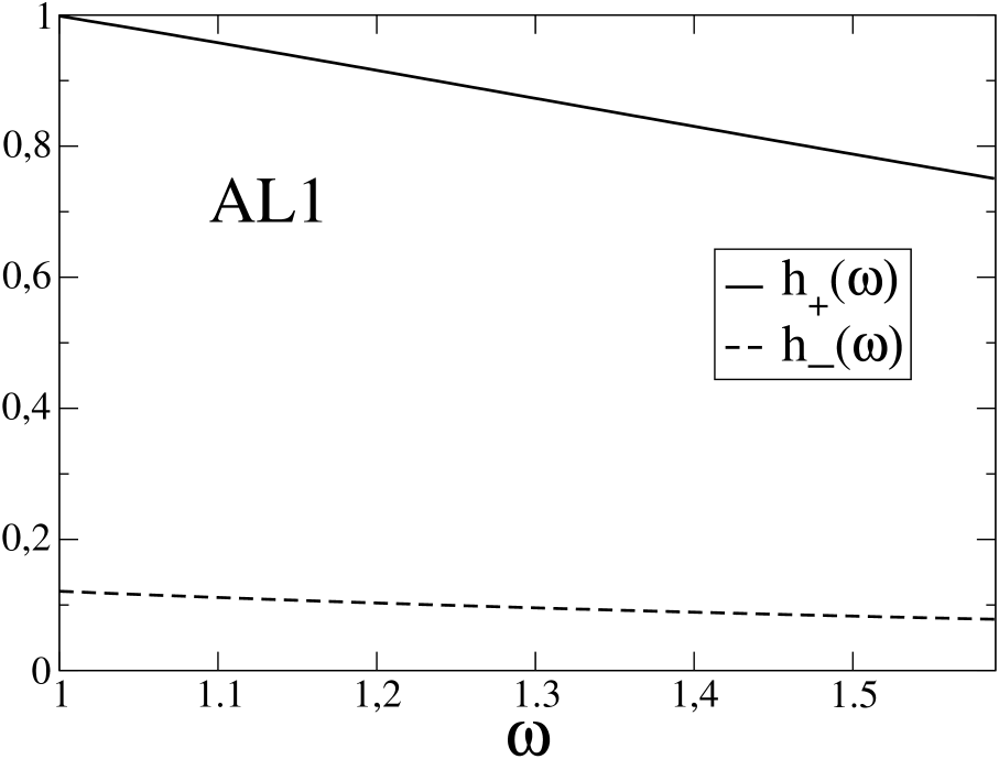
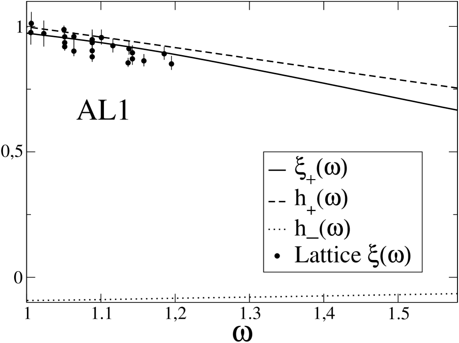
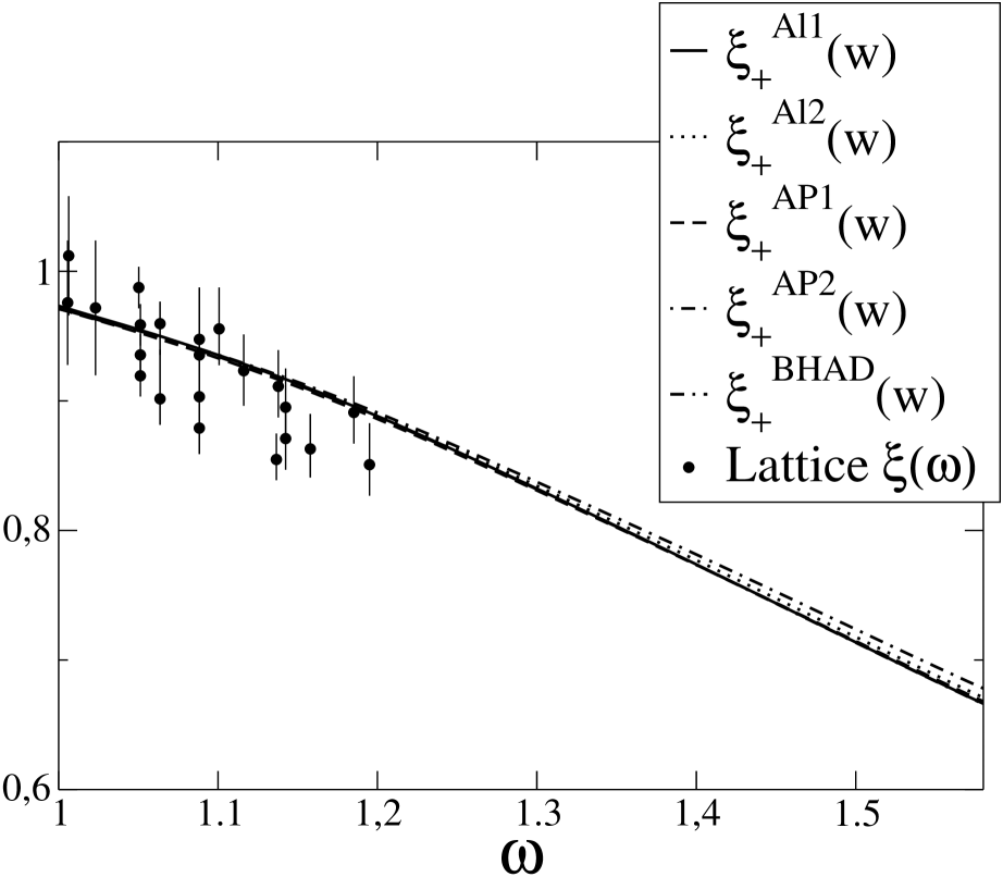
Figure 3.1: Top panel: $h_{+}(w)$ and $h_{-}(w)$ for the $B\to D$ transition as obtained from Eqs. (3.4.1, 3.4.1) using the AL1 interquark potential. Middle panel: $h_{+}(w)$ as before, $\xi_{+}(w)$ obtained from the values of $h_{+}(w)$ using Eq. (3.22), $h_{-}(w)$ obtained from $\xi_{+}(w)$ using Eq. (3.22). We also show the UKQCD lattice data by Bowler et al. [137]. Lower panel: Different $\xi_{+}(w)$ obtained with the above procedure for the different interquark interactions. Lattice data is also shown.

In the top panel of Fig. 3.1 we show the values of $h_{+}(w)$ and $h_{-}(w)$ for the $B\to D$ transition as obtained from Eqs. (3.4.1, 3.4.1) with the use of the AL1 interquark potential. The values for $h_{-}(w)$ are not reliable. Actual calculation shows that they are of the same size as the deviations from zero that one computes in the equal mass case. To improve on this what we shall do instead is to use the form factor $h_{+}(w)$ and Eq. (3.22) to extract $\xi(w)$ (we shall call it $\xi_{+}(w)$ ) and from there we can re-evaluate $h_{-}(w)$ with the use of Eq. (3.22). The results appear in the middle panel of Fig. 3.1 where we also show the lattice results for $\xi(w)$ obtained by the UKQCD Collaboration in Ref. [137]. We find good agreement with lattice data. Finally in the lower panel of Fig. 3.1 we show the different $\xi_{+}(w)$ obtained with the use of the different interquark potentials. As we see from the figure all $\xi_{+}(w)$ are very much the same in the whole interval for $w$.

The slope at the origin of our Isgur-Wise function is given by

$$\rho^{2}=-\frac{1}{\xi_{+}(w)}\left.\frac{d\,\xi_{+}(w)}{dw}\right|_{w=1}=0.35\pm 0.02$$ (3.29)

small compared to the lattice value of $\rho^{2}=0.81^{+17}_{-11}$ extracted from a best fit to data.

Differential decay width

Neglecting lepton masses the differential decay width for the process $B\to D\,l\,\bar{\nu}$ is given by [138]

$$\frac{d\Gamma}{dw}=\frac{G_{F}^{2}}{48\pi^{3}}\,|V_{cb}|^{2}\,m_{D}^{3}\,(w^{2}-1)^{3/2}(m_{B}+m_{D})^{2}\ F_{D}^{2}(w)$$ (3.30)

where $G_{F}=1.16637(1)\times 10^{-5}$  GeV^-2 [115] is the Fermi decay constant, $V_{cb}$ is the CKM matrix element for the $b\to c$ weak transition, and $F_{D}(w)$ is given by

$$F_{D}(w)=\bigg{[}h_{+}(w)-\frac{1-r}{1+r}\,h_{-}(w)\bigg{]}$$ (3.31)

with $r=m_{D}/m_{B}$.

In Fig. 3.2 we show our calculation for $F_{D}(w)\ |V_{cb}|$ obtained with the AL1 interquark potential and using three different values of $|V_{cb}|$ corresponding to the central and extreme values of the range for $|V_{cb}|$ favored by the Particle Data Group (PDG), $|V_{cb}|=0.039\sim 0.044$ [115]. We also show the experimental data for the decays $B^{-}\to D^{0}\,l\,\bar{\nu}$ and $\bar{B}^{0}\to D^{+}\,l\,\bar{\nu}$ obtained by the CLEO Collaboration [139], a fit to CLEO data using the form factors of Boyd et al. [140], and the experimental data for the decay $\bar{B}^{0}\to D^{+}\,l\,\bar{\nu}$ obtained by the BELLE Collaboration [141]. Our results are larger than experimental data for $w>1.2$. Our total integrated width will thus be larger than the experimental one for any reasonable value of $|V_{cb}|$.

Figure 3.2: $F_{D}(r,w)\ |V_{cb}|$ obtained with the AL1 interquark potential. Solid line: our results using $|V_{cb}|=0.0415$. Dashed line: our results using $|V_{cb}|=0.044$. Dotted line: our results using $|V_{cb}|=0.039$. Circles: experimental data by the CLEO Collaboration [139]. Dashed-dotted line: fit to CLEO data using the form factors of Boyd et al. [140]. Diamonds: experimental data the by BELLE Collaboration [141].

From our data we extract the slope at $w=1$ given by

$$\rho_{D}^{2}=\left.-\frac{1}{F_{D}(w)}\frac{dF_{D}(w)}{dw}\right|_{w=1}=0.38\pm 0.02$$ (3.32)

which is small compared to the values extracted from the experimental data: $\rho_{D}^{2}=0.76\pm 0.16\pm 0.08$ [139] and $\rho_{D}^{2}=0.69\pm 0.14$ [141] obtained from a linear fit to the data, or $\rho_{D}^{2}=1.30\pm 0.27\pm 0.14$ [139] and $\rho_{D}^{2}=1.16\pm 0.25$ [141] obtained using the form factors of Boyd et al. [140]. Thus, only our results close to $w=1$ seem to be reliable. We can use our prediction for $F_{D}(1)$ to extract the value of $|V_{cb}|$ from the experimental determination of the quantity $|V_{cb}|F_{D}(1)$. Different values of that quantity appear in Table 3.5.

	$|V_{cb}|\,F_{D}(1)$
CLEO Collaboration  [139]	$\ 0.0416\pm 0.0047\pm 0.0037$
BELLE Collaboration  [141]	$\ 0.0411\pm 0.0044\pm 0.0052$

Table 3.5: $|V_{cb}|\,F_{D}(1)$ values obtained by different experiments.

Our result for $F_{D}(1)$ is given by (we do not show the theoretical error which is or the order of $10^{-4}$)

$$F_{D}(1)=1.04$$ (3.33)

which is in good agreement with other calculations $F_{D}(1)=0.98\pm 0.07$ [142], $F_{D}(1)=1.04$ [83] or $F_{D}(1)=1.069\pm 0.008\pm 0.002\pm 0.025$ [143]. From our value for $F_{D}(1)$ and the experimental values for $|V_{cb}|F_{D}(1)$ we can obtain $|V_{cb}|$ in the range

$$|V_{cb}|=0.040\pm 0.006$$ (3.34)

This result agrees with a recent determination based on the analysis of the $\Lambda_{b}\to\Lambda_{c}\,l\,\bar{\nu}_{l}$ reaction using the same model, from where $|V_{cb}|=0.040\pm 0.005$ was obtained [144].

3.4.2 $B\to D^{*}\,l\,\bar{\nu}$ decay

Working again in the center of mass of the $B$ meson and taking $\vec{P}^{\,\prime}=-\vec{q}=-|\vec{q}\,|\,{\vec{k}}$ in the z direction we will have for the form factors $h_{V}(w)$, $h_{A_{1}}(w)$, $h_{A_{2}}(w)$ and $h_{A_{3}}(w)$ the expressions

$$h_{V}(w) = \sqrt{2}\,\sqrt{\frac{m_{D^{*}}}{m_{B}}}\,\frac{V^{(*)}_{-1,\,2}(|\vec{q}\,|)}{|\vec{q}\,|}$$

$$h_{A_{1}}(w) = i\,\frac{\sqrt{2}}{w+1}\,\frac{1}{\sqrt{m_{B}m_{D^{*}}}}\,A^{(*)}_{-1,\,1}(|\vec{q}\,|)$$

$$h_{A_{2}}(w) = i\,\sqrt{\frac{m_{D^{*}}}{m_{B}}}\,\left(-\frac{A^{(*)}_{0,\,0}(|\vec{q}\,|)}{|\vec{q}\,|}+\frac{E_{D^{*}}(-\vec{q})\,A^{(*)}_{0,\,3}(|\vec{q}\,|)}{|\vec{q}\,|^{2}}-\sqrt{2}\,m_{D^{*}}\frac{A^{(*)}_{-1,\,1}(|\vec{q}\,|)}{|\vec{q}\,|^{2}}\right)$$

$$h_{A_{3}}(w) = i\frac{m_{D^{*}}^{2}}{\sqrt{m_{B}m_{D^{*}}}}\left(-\frac{A^{(*)}_{0,\,3}(|\vec{q}\,|)}{|\vec{q}\,|^{2}}+\,\frac{\sqrt{2}}{m_{D^{*}}}\frac{E_{D^{*}}(-\vec{q})\,A^{(*)}_{-1,\,1}(|\vec{q}\,|)}{|\vec{q}\,|^{2}}\right)$$ (3.35)

with $E_{D^{*}}(-\vec{q})=\sqrt{m_{D^{*}}^{2}+\vec{q}\,^{2}}$, and where $V^{(*)}_{\lambda,\,\mu}(|\vec{q}\,|)$ and $A^{(*)}_{\lambda,\,\mu}(|\vec{q}\,|)$ are given by

$$V^{(*)}_{\lambda,\,\mu}(|\vec{q}\,|)=\left\langle\,D^{*},\,\lambda\ -|\vec{q}\,|\,\vec{k}\,\left|\,(J^{c\,b}_{V})_{\mu}(0)\,\right|\,B,\,\vec{0}\right\rangle$$

$$A^{(*)}_{\lambda,\,\mu}(|\vec{q}\,|)=\left\langle\,D^{*},\,\lambda\ -|\vec{q}\,|\,\vec{k}\,\left|\,(J^{c\,b}_{A})_{\mu}(0)\,\right|\,B,\,\vec{0}\right\rangle$$ (3.36)

In our model $V^{(*)}_{\lambda,\,\mu}(|\vec{q}\,|)$ and $A^{(*)}_{\lambda,\,\mu}(|\vec{q}\,|)$ are evaluated as

$$V^{(*)}_{\lambda,\,\mu}(|\vec{q}\,|) = \sqrt{2m_{B}2E_{D^{*}}(-\vec{q})}\ \ {}_{\stackrel{{\scriptstyle}}{{NR}}}\left\langle\,D^{*},\,\lambda\ -|\vec{q}\,|\,{\vec{k}}\,\left|\,(J^{c\,b}_{V})_{\mu}(0)\,\right|\,B,\,\vec{0}\right\rangle_{NR}$$

$$A^{(*)}_{\lambda,\,\mu}(|\vec{q}\,|) = \sqrt{2m_{B}2E_{D^{*}}(-\vec{q})}\ \ {}_{\stackrel{{\scriptstyle}}{{NR}}}\left\langle\,D^{*},\,\lambda\ -|\vec{q}\,|\,{\vec{k}}\,\left|\,(J^{c\,b}_{A})_{\mu}(0)\,\right|\,B,\,\vec{0}\right\rangle_{NR}$$

with expressions given in appendix D.

In the top panel of Fig. 3.3 we show our results for the $h_{V}(w),h_{A_{1}}(w),h_{A_{2}}(w)$ and $h_{A_{3}}(w)$ form factors, obtained with the AL1 interquark potential and the use of Eq. (3.4.2). In the lower panel of the same figure we show the ratios

Figure 3.3: Top panel: $h_{V}(w)$, $h_{A_{1}}(w)$, $h_{A_{2}}(w)$ and $h_{A_{3}}(w)$ form factors obtained using Eq. (3.4.2). Lower panel: $R_{1}(w)$ and $R_{2}(w)$ ratios. In both panels the AL1 interquark potential has been used.

$$R_{1}(w)=\frac{h_{V}(w)}{h_{A_{1}}(w)}$$

$$R_{2}(w)=\frac{h_{A_{3}}(w)+r\,h_{A_{2}}(w)}{h_{A_{1}}(w)}$$ (3.38)

where now $r=m_{D^{*}}/m_{B}$. These ratios are expected to vary very weakly with $w$. We find indeed that this is so in our case being our values of $R_{1}(w)$ and $R_{2}(w)$ within 4% of unity. In Table 3.6 we give now our results for $R_{1}(1)$ and $R_{2}(1)$ and compare them to different experimental and theoretical determinations. We find discrepancies of the order of $15\sim 33\,\%$ for $R_{1}(1)$ and $13\sim 46\,\%$ for $R_{2}(1)$.

One can understand these discrepancies by evaluating the different $\xi(w)$ functions obtained from the form factors with the use of Eq. (3.22) and the $\beta$ and $\gamma$ coefficients of Neubert given in Tables 3.3 and 3.4. The results appear in the top panel of Fig. 3.4. One can infer from the figure that our results for $h_{A_{2}}(w)$ are not reliable. Also we somehow miss the correct normalization for $h_{V}(1)$. On the other hand the values of $\xi_{A_{1}}(w)$ and $\xi_{A_{3}}(w)$ are equal within 4% and in reasonable agreement with lattice data from Ref. [137].

To improve the nonrelativistic quark model prediction, and similarly to what we did in subsection 3.4.1, we will take $\xi_{A_{1}}(w)$ as our model determination of the Isgur-Wise function $\xi(w)$ and we will reevaluate the form factors with the use of Eq. (3.22). What we obtain is now depicted in the middle panel of Fig. 3.4. In the lower panel we give the different $\xi_{A_{1}}(w)$ obtained with the different interquark potentials. They do not show any significant difference.

The slope of the $\xi_{A_{1}}(w)$ function at the origin is given by

$$\rho^{2}=0.55\pm 0.02$$ (3.39)

to be compared to the lattice result $\rho^{2}=0.93^{+47}_{-59}$ [137]. In this case we are within lattice errors, but one can not be very conclusive due to the large value of the latter in this case.

	$R_{1}(1)$	$R_{2}(1)$
This work	$1.01\pm 0.02$	$1.04\pm 0.01$
CLEO [145]	$1.18\pm 0.30\pm 0.12$	$0.71\pm 0.22\pm 0.07$
BABAR (Preliminary) [146]	$1.328\pm 0.055\pm 0.025\pm 0.025$	$0.920\pm 0.044\pm 0.020\pm 0.013$
Caprini et al. [147]	1.27	0.80
Grinstein et al. [148]	1.25	0.81
Close et al. [103]	1.15	0.91

Table 3.6: $R_{1}(1)$ and $R_{2}(1)$

Figure 3.4: Top panel: different $\xi(w)$ functions obtained from the $h_{V}(w)$, $h_{A_{1}}(w)$, $h_{A_{2}}(w)$ and $h_{A_{3}}(w)$ form factors using Eq. (3.22) and the AL1 interquark potential. Lattice data by K. C. Bowler et al. from Ref. [137] are also shown. Middle panel: form factors obtained from $\xi_{A_{1}}(w)$ with the use of Eq. (3.22). Lower panel: Different $\xi_{A_{1}}(w)$ obtained with the different interquark potentials.

Finally in Fig. 3.5 we give the ratio $\xi_{+}(w)/\xi_{A_{1}}(w)$ evaluated with the AL1 interquark potential. We see the differences between the two Isgur-Wise functions are at the level of 3-7%.

Figure 3.5: Ratio of our two Isgur-Wise functions calculated with the AL1 interquark potential.

Differential decay width

Neglecting lepton masses the differential decay width for the process $B\to D^{*}\,l\,\bar{\nu}$ is given by [149]

$$\frac{d\Gamma}{dw}=\frac{G_{F}^{2}}{48\pi^{3}}\,|V_{cb}|^{2}\,(m_{B}-m_{D^{*}})^{2}\,m_{D^{*}}^{3}\,\sqrt{(w^{2}-1)}\,(w+1)^{2}$$

$$\hskip 142.26378pt\times\bigg{[}1+\frac{4w}{w+1}\ \frac{1-2wr+r^{2}}{(1-r)^{2}}\bigg{]}\ F_{D^{*}}^{2}(w)$$ (3.40)

where $F_{D^{*}}(w)$ is defined as

$$F_{D^{*}}(w)=h_{A_{1}}(w)\sqrt{\frac{\tilde{H}_{0}^{2}(w)+\tilde{H}_{+}^{2}(w)+\tilde{H}_{-}^{2}(w)}{1+\frac{4w}{w+1}\ \frac{1-2wr+r^{2}}{(1-r)^{2}}}}$$ (3.41)

The $\tilde{H}_{j}(w)$ are helicity form factors given in terms of the $R_{1}(w)$ and $R_{2}(w)$ ratios as

$$\tilde{H}_{0}(w) = 1+\frac{w-1}{1-r}\,[1-R_{2}(w)]$$

$$\tilde{H}_{\pm}(w) = \frac{\sqrt{1-2wr+r^{2}}}{1-r}\left[1\mp\sqrt{\frac{w-1}{w+1}}\ R_{1}(w)\right]$$ (3.42)

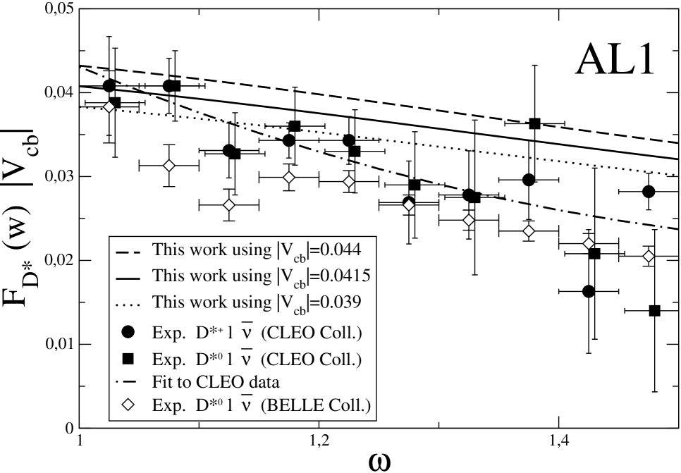
Figure 3.6: $F_{D^{*}}(r,w)\ |V_{cb}|$ obtained with the AL1 interquark potential. Solid line: our results using $|V_{cb}|=0.0415$. Dashed line: our results using $|V_{cb}|=0.044$. Dotted line: our results using $|V_{cb}|=0.039$. Circles and squares: experimental data by the CLEO Collaboration [145]. Dashed-dotted line: fit to CLEO Collaboration data. Diamonds: experimental data by the BELLE Collaboration [141].

Similarly to Fig. 3.2, in Fig. 3.6 we show our results for the quantity $F_{D^{*}}(w)\ |V_{cb}|$ evaluated with the AL1 interquark potential and using the values of $|V_{cb}|$ corresponding to the central and extreme values of the range for $|V_{cb}|$ favored by the PDG. We also show the experimental data by the CLEO Collaboration [145] for the $B^{-}\to D^{*0}\,l\,\bar{\nu}$ reaction (squares), and for the $\bar{B}^{0}\to D^{*+}\,l\,\bar{\nu}$ reaction (circles) together with a best fit, and the experimental data by the BELLE Collaboration [150] for the $\bar{B}^{0}\to D^{*+}\,l\,\bar{\nu}$ reaction (diamonds). We find good agreement with CLEO data for small $w$ values. Disagreement starts already at around $w=1.1$ where our results start to go above the experimental data. BELLE data are systematically below our results.

Also our slope at the origin

$$\rho^{2}_{D^{*}}=-\frac{1}{F_{D^{*}}(w)}\left.\frac{dF_{D^{*}}(w)}{dw}\right|_{w=1}=0.31\pm 0.02$$ (3.43)

is smaller than the value obtained by the BELLE Collaboration $\rho^{2}_{D^{*}}=0.81\pm 0.12$ [150] using a linear fit to their data. All this means that our total width would be larger than the experimental one for any reasonable value of $V_{cb}$. On the other hand experimentalists are able to extract the value of $|V_{cb}|\,F_{D^{*}}(1)$. Different experimental results for that quantity appear in Table 3.7.

	$|V_{cb}|\,F_{D^{*}}(1)$
(CLEO Coll.)  [145]	$\ 0.0431\pm 0.0013\pm 0.0018$
(DELPHI Coll.)  [151]	$\ 0.0392\pm 0.0018\pm 0.0023$
(BELLE Coll.)  [150]	$\ 0.0354\pm 0.0019\pm 0.0018$
(BABAR Coll.)  [152]	$\ 0.0355\pm 0.0003\pm 0.0016$

Table 3.7: $|V_{cb}|\,F_{D^{*}}(1)$ values obtained by different experiments.

Our result for $F_{D^{*}}(1)$ is given by

$$F_{D^{*}}(1)=h_{A_{1}}(1)=0.983\pm 0.001$$ (3.44)

Comparison with the experimental data for $|V_{cb}|\,F_{D^{*}}(1)$ allows us to extract values for $|V_{cb}|$ in the range

$$|V_{cb}|=0.0333\sim 0.0461$$ (3.45)

One can not be more conclusive due to the dispersion in the experimental data for $|V_{cb}|\,F_{D^{*}}(1)$. From DELPHI data alone we would obtain $|V_{cb}|=0.040\pm 0.003$ in perfect agreement with our determination using the $B\to D$ reaction data. We should also say that our value for $F_{D^{*}}(1)$ is larger than the lattice determination $F_{D^{*}}(1)=0.919^{+0.030}_{-0.035}$ by S. Hashimoto et al. [153] normally used by experimentalists to extract their $|V_{cb}|$ values. A new unquenched lattice determination of this quantity by the Fermilab Lattice Collaboration is in progress [132].

3.5 Strong coupling constants $g_{H^{*}H\pi}$

In this section we will evaluate the strong coupling constants $g_{H^{*}H\pi}$ where $H$ stands for a $B$ or $D$ meson. To this end we shall make use of the partial conservation of the axial current hypothesis (PCAC) which relates the divergence of the axial current to the pion field as

$$\partial^{\mu}\,J_{A\,\mu}^{d\,u}(x)=\,f_{\pi}\,m_{\pi}^{2}\,\Phi_{\pi^{-}}(x)$$ (3.46)

where $f_{\pi}=130.7\pm 0.1\pm 0.36$ MeV [115] is the pion decay constant, $m_{\pi}=139.57$ MeV [115] is the pion mass, and $\Phi_{\pi^{-}}(x)$ is the charged pion field that destroys a $\pi^{-}$ and creates a $\pi^{+}$. Using the Lehmann-Symanzik-Zimmermann reduction formula one can relate the matrix element of the divergence of the axial current to the pion emission amplitude as

$$\langle H,\ \vec{P}^{\prime}\,|\,q^{\mu}\,J_{A\,\mu}^{d\,u}(0)\,|\,H^{*},\lambda\,\vec{P}\,\rangle=-i\,f_{\pi}\frac{m_{\pi}^{2}}{q^{2}-m_{\pi}^{2}}\ {\cal A}^{(\lambda)}_{H^{*}H\pi}(P^{\prime},P)$$ (3.47)

where $q=P-P^{\prime}$ and ${\cal A}^{(\lambda)}_{H^{*}H\pi}(P^{\prime},P)$ is the pion emission amplitude for the process $H^{*}\to H\pi$ given by

$${\cal A}^{(\lambda)}_{H^{*}H\pi}(P^{\prime},P)=-\,g_{H^{*}H\pi}(q^{2})\,\left(q\cdot\varepsilon_{(\lambda)}(\vec{P}\,)\right)$$ (3.48)

The matrix element on the left hand side of Eq.(3.47) has a pion pole contribution that can be easily evaluated to be

$$\langle H,\ \vec{P}^{\prime}\,|\,q^{\mu}\,J_{A\,\mu}^{d\,u}(0)\,|\,H^{*},\lambda\,\vec{P}\,\rangle_{pion-pole}=-i\,f_{\pi}\frac{q^{2}}{q^{2}-m_{\pi}^{2}}\ {\cal A}^{(\lambda)}_{H^{*}H\pi}(P^{\prime},P)$$

so that we can extract a non-pole contribution

$$\langle H,\ \vec{P}^{\prime}\,|\,q^{\mu}\,J_{A\,\mu}^{d\,u}(0)\,|\,H^{*},\lambda\,\vec{P}\,\rangle_{non-pole} = i\,f_{\pi}\ {\cal A}^{(\lambda)}_{H^{*}H\pi}(P^{\prime},P)$$

$$= -i\,f_{\pi}\ g_{H^{*}H\pi}(q^{2})\,\left(q^{\mu}\,\varepsilon_{(\lambda)\mu}(\vec{P}\,)\right)$$

which is the one we shall evaluate within the quark model. For the matrix element on the left hand side of Eq.(3.5) we can use a parametrization similar to the one used in Eq.(3.4)

$$\langle H,\ \vec{P}^{\prime}\,|\,q^{\mu}\,J_{A\,\mu}^{d\,u}(0)\,|\,H^{*},\lambda\,\vec{P}\,\rangle_{non-pole}=$$

$$q^{\mu}\bigg{\{}-i\,\varepsilon_{(\lambda)\mu}(\vec{P}\,)\ (w+1)\ h_{A_{1}}(w)$$

$$+i\left(\varepsilon_{(\lambda)}(\vec{P}\,)\cdot v^{\prime}\right)\left(v^{\prime}_{\mu}\,h_{A_{2}}(w)+v_{\mu}\,h_{A_{3}}(w)\right)\bigg{\}}\sqrt{m_{H}m_{H^{*}}}$$ (3.51)

with the result that

$$g_{H^{*}H\pi}(q^{2})=\frac{1}{f_{\pi}}\bigg{\{}(w+1)\,h_{A_{1}}(w)+w\left(\frac{m_{H^{*}}}{m_{H}}\,h_{A_{2}}(w)-h_{A_{3}}(w)\right)$$

$$+\left(\frac{m_{H^{*}}}{m_{H}}\,h_{A_{3}}(w)-h_{A_{2}}(w)\right)\bigg{\}}\sqrt{m_{H}m_{H^{*}}}$$ (3.52)

The evaluation of the form factors is done is a similar way as the one described in subsection 3.4.2. The results that we get for $q^{2}=0$ are

$$g_{D^{*}D\pi}(0)=22.1\pm 0.4\hskip 14.22636pt,\hskip 14.22636ptg_{B^{*}B\pi}(0)=60.5\pm 1.1$$ (3.53)

to be compared to the experimental determination $g_{D^{*}D\pi}(m_{\pi}^{2})=17.9\pm 0.3\pm 1.9$ by the CLEO Collaboration [154], the lattice results $g_{D^{*}D\pi}(m_{\pi}^{2})=18.8\pm 2.3^{+1.1}_{-2.0}$ [155] and $g_{B^{*}B\pi}(0)=47\pm 5\pm 8$ [156], or a recent determination using QCDSR for which $g_{D^{*}D\pi}(m_{\pi}^{2})=14.0\pm 1.5$ and $g_{B^{*}B\pi}(0)=42.5\pm 2.6$ [157]. Older QCDSR results give smaller values for both coupling constants. For instance, the calculation within QCDSR on the light cone in Ref. [158] give $g_{D^{*}D\pi}(m_{\pi}^{2})=12.5\pm 1$ and $g_{B^{*}B\pi}(0)=29\pm 3$ . The latter are small compared to lattice data or the experimental determination of $g_{D^{*}D\pi}(m_{\pi}^{2})$ by the CLEO Collaboration.

From our results we obtain the ratio

$$R=\frac{g_{B^{*}B\pi}(0)\ f_{B^{*}}\,\sqrt{m_{D}}}{g_{D^{*}D\pi}(0)\ f_{D^{*}}\,\sqrt{m_{B}}}=1.105\pm 0.005$$ (3.54)

in good agreement with HQS that predicts a value of 1 with $1/m_{c,b}$ corrections appearing in next to leading order [133] . Our result in Eq.(3.54) is also in agreement with the one obtained combining lattice data for $f_{B^{*}}$ and $f_{D^{*}}$ from Ref. [118], for $g_{B^{*}B\pi}(0)$ from Ref. [155], and the experimental CLEO Collaboration data for $g_{D^{*}D\pi}(m_{\pi}^{2})$ from Ref. [154]. In this case one gets

$$\left.R\right|_{Exp.-Latt.}=1.26\pm 0.36$$ (3.55)

where we have added errors in quadratures. A calculation using light cone QCDSR gives [158]

$$\left.R\right|_{QCDSR}=0.92$$ (3.56)

Chapter 4 Semileptonic and non-leptonic decays of the $B_{c}^{-}$ meson

4.1 Introduction

Since its discovery at Fermilab by the CDF Collaboration [159, 160] the $B_{c}$ meson has drawn a lot of attention. Unlike other heavy mesons it is composed of two heavy quarks of different flavor ($b,\,c$) and, being below the $B$–$D$ threshold, it can only decay through weak interactions making an ideal system to study weak decays of heavy quarks.

Using HQSS Jenkins et al. [72] were able to obtain, in the infinite heavy quark mass limit, relations between different form factors for semileptonic $B_{c}$ decays into pseudoscalar and vector mesons. Contrary to the heavy-light meson case where standard HQS applies, no determination of corrections in inverse powers of the heavy quark masses has been worked out in this case. So one can only test any model calculation against HQSS predictions in the infinite heavy quark mass limit.

With both quarks being heavy, a nonrelativistic treatment of the $B_{c}$ meson should provide reliable results. Besides a nonrelativistic model will comply with the constraints imposed by HQSS as the spin–spin interaction vanish in the infinity heavy quark mass limit. In this chapter we will study, within the framework of a nonrelativistic quark model, exclusive semileptonic and nonleptonic decays of the $B_{c}^{-}$ meson driven by a $b\to c$ or $\bar{c}\to\bar{d},\,\bar{s}$ transitions at the quark level. We will not consider semileptonic processes driven by the quark $b\to u$ transition. Our experience with this kind of processes, like the analogous $B\to\pi$ semileptonic decay  [161], shows that the nonrelativistic model without any improvements underestimates the decay width for two reasons: first at high $q^{2}$ transfers one might need to include the exchange of a $B^{*}$ meson, and second the model underestimates the form factors at low $q^{2}$ or high three–momentum transfers. We will concentrate thus on semileptonic $B_{c}^{-}\to c\bar{c}$ and $B_{c}^{-}\to\overline{B}$ transitions. As for two–meson nonleptonic decay we will only consider channels with a least a $c\bar{c}$ or $B$ final meson. In the first case we will include channels with final $D$ mesons for which there is a contribution coming from an effective $b\to d,\,s$ transition. As later explained this is not the main contribution to the decay amplitude and besides the momentum transfer in those cases is neither too high nor too low so that the problems mentioned above are avoided.

The observables studied here have been analyzed before in the context of different models like the relativistic constituent quark model [162, 163, 164], the quasi-potential approach to the relativistic quark model [165, 166], the instantaneous nonrelativistic approach to the Bethe–Salpeter equation [167, 168, 169], the Bethe–Salpeter equation [170, 171], the three point sum rules of QCD and nonrelativistic QCD [172, 173, 174, 175], the QCD relativistic potential model [176], the relativistic constituent quark model formulated on the light front [177], the relativistic quark–meson model [178] or in models that use the Isgur, Scora, Grinstein and Wise wave functions [82, 83] like the calculations in Refs. [179, 180, 181]. We will compare our results with those obtained in these latter references whenever is possible. Besides, we will perform an exhaustive study for exclusive semileptonic and nonleptonic $B_{c}^{-}$ decays, paying an special attention to the theoretical uncertainties affecting our predictions and providing reliable estimates for all of them.

In the present calculation we shall use physical masses taken from Ref. [115]. For the $B_{c}$ meson mass and lifetime we shall use the central values of the recent experimental determinations by the CDF Collaboration of $m_{B_{c}}=6285.7\pm 5.3\pm 1.2$ MeV/$c^{2}$ [182] and $\tau_{B_{c}}=(0.463^{+0.073}_{-0.065}\pm 0.036)\times 10^{-12}$ s  [183]. This new mass value is very close to the one we obtain with the different quark-quark potentials that we use in this memory from where we get $m_{B_{c}}=6291.6^{+12}_{-33}$ MeV.

We shall also need CKM matrix elements and different meson decay constants. For the former we shall use the ones quoted in Ref. [162] that we reproduce in Table 4.1. All of them are within the ranges quoted by the Particle Data Group (PDG) [115].

$|V_{ud}|$	$|V_{us}|$	$|V_{cd}|$	$|V_{cs}|$	$|V_{cb}|$
0.975	0.224	0.224	0.974	0.0413

Table 4.1: Values for Cabibbo-Kobayashi-Maskawa matrix elements used in this work.

For the meson decay constants the values used in this work are compiled in Table 4.2. They correspond to central values of experimental measurements or lattice determinations. The results for $f_{\rho}$ and $f_{K^{*}}$ have been obtained by the authors in Ref. [162] using $\tau$ lepton decay data. Our own theoretical calculation, obtained with the model described chapter 3, give $f_{\rho}=0.189\sim 0.227$ GeV, $f_{K^{*}}=0.180\sim 0.220$ GeV depending on the inter-quark interaction used, results which agree with the determinations in Ref. [162]. We shall nevertheless use the latter for our calculations. For $f_{\eta_{c}}$ we have been unable to find an experimental result or a lattice determination. There are at least two theoretical determinations that predict $f_{\eta_{c}}=0.484$ GeV [162] and $f_{\eta_{c}}=0.420\pm 0.052$ GeV [185]. Again our own calculation gives values in the range $f_{\eta_{c}}=0.485\sim 0.500$ GeV depending on the inter-quark interaction used. Here we will take $f_{\eta_{c}}=0.490$ GeV.

$f_{\pi^{-}}$	$f_{\pi^{0}}$	$f_{\rho^{-},\,\rho^{0}}$	$f_{K^{-},\,K^{0}}$	$f_{K^{*-},\,K^{*0}}$
0.1307 [115]	0.130 [115]	0.210 [162]	0.1598 [115]	0.217 [162]

$f_{\eta_{c}}$	$f_{J/\Psi}$
0.490	0.405 [186]

$f_{D^{-}}$	$f_{D^{*-}}$	$f_{D_{s}^{-}}$	$f_{D_{s}^{*-}}$
0.2226 [123]	0.245 [187]	0.294 [188]	0.272 [187]

Table 4.2: Meson decay constants in GeV used in this work.

4.2 Meson states

The meson states were introduced earlier in chapter 3. Here we will need the ground state wave function for scalar ($0^{+}$), pseudoscalar ($0^{-}$), vector ($1^{-}$), axial vector ($1^{+}$), tensor ($2^{+}$) and pseudotensor ($2^{-}$) mesons. Assuming always the lowest possible value for the orbital angular momentum we will have for a meson $M$ with scalar, pseudoscalar and vector quantum numbers:

$$\hat{\phi}^{\,(0^{+})}_{\alpha_{1},\,\alpha_{2}}(\,\vec{p}\,) = \frac{1}{\sqrt{3}}\,\delta_{c_{1},\,c_{2}}\ \hat{\phi}^{\,(0^{+})}_{(s_{1},\,f_{1}),\,(s_{2},\,f_{2})}(\,\vec{p}\,)$$

$$= \frac{1}{\sqrt{3}}\,\delta_{c_{1},\,c_{2}}\ i\ \hat{\phi}^{\,(0^{+})}_{f_{1},\,f_{2}}(\,|\vec{p}\,|)$$

$$\hskip 19.91684pt\sum_{m}\ \left(\left.\frac{1}{2},\frac{1}{2},1\right|s_{1},s_{2},-m\right)\ \left(\left.1,1,0\right|m,-m,0\right)\ Y_{1m}(\,{\vec{p}}\ )$$

$$\hat{\phi}^{\,(0^{-})}_{\alpha_{1},\,\alpha_{2}}(\,\vec{p}\,) = \frac{1}{\sqrt{3}}\,\delta_{c_{1},\,c_{2}}\ \hat{\phi}^{\,(0^{-})}_{(s_{1},\,f_{1}),\,(s_{2},\,f_{2})}(\,\vec{p}\,)$$

$$= \frac{1}{\sqrt{3}}\,\delta_{c_{1},\,c_{2}}\ (-i)\ \hat{\phi}^{\,(0^{-})}_{f_{1},\,f_{2}}(\,|\vec{p}\,|)\ \left(\left.\frac{1}{2},\frac{1}{2},0\right|s_{1},s_{2},0\right)\ Y_{00}(\,{\vec{p}}\ )$$

$$\hat{\phi}^{\,(1^{-},\,\lambda)}_{\alpha_{1},\,\alpha_{2}}(\,\vec{p}\,) = \frac{1}{\sqrt{3}}\,\delta_{c_{1},\,c_{2}}\ \hat{\phi}^{\,(1^{-},\,\lambda)}_{(s_{1},\,f_{1}),\,(s_{2},\,f_{2})}(\,\vec{p}\,)$$

$$= \frac{1}{\sqrt{3}}\,\delta_{c_{1},\,c_{2}}\ (-1)\ \hat{\phi}^{\,(1^{-})}_{f_{1},\,f_{2}}(\,|\vec{p}\,|)\ \left(\left.\frac{1}{2},\frac{1}{2},1\right|s_{1},s_{2},\lambda\right)\ Y_{00}(\,{\vec{p}}\ )$$

For axial mesons we need orbital angular momentum $L=1$. In this case two values of the total quark–antiquark spin $S_{q\bar{q}}=0,1$ are possible, giving rise to the two states:

$$\hat{\phi}^{\,((1^{+},S_{q\bar{q}}=0),\,\lambda)}_{\alpha_{1},\,\alpha_{2}}(\,\vec{p}\,) = \frac{1}{\sqrt{3}}\,\delta_{c_{1},\,c_{2}}\ \hat{\phi}^{\,((1^{+},S_{q\bar{q}}=0),\,\lambda)}_{(s_{1},\,f_{1}),\,(s_{2},\,f_{2})}(\,\vec{p}\,)$$

$$= \frac{1}{\sqrt{3}}\,\delta_{c_{1},\,c_{2}}\ (-1)\ \hat{\phi}^{\,(1^{+},S_{q\bar{q}}=0)}_{f_{1},\,f_{2}}(\,|\vec{p}\,|)\ \left(\left.\frac{1}{2},\frac{1}{2},0\right|s_{1},s_{2},0\right)\ Y_{1\lambda}(\,{\vec{p}}\ )$$

$$\hat{\phi}^{\,((1^{+},S_{q\bar{q}}=1),\,\lambda)}_{\alpha_{1},\,\alpha_{2}}(\,\vec{p}\,) = \frac{1}{\sqrt{3}}\,\delta_{c_{1},\,c_{2}}\ \hat{\phi}^{\,((1^{+},S_{q\bar{q}}=1),\,\lambda)}_{(s_{1},\,f_{1}),\,(s_{2},\,f_{2})}(\,\vec{p}\,)$$

$$= \frac{1}{\sqrt{3}}\,\delta_{c_{1},\,c_{2}}\ (-1)\ \hat{\phi}^{\,(1^{+},S_{q\bar{q}}=1)}_{f_{1},\,f_{2}}(\,|\vec{p}\,|)$$

$$\times\sum_{m}\ \left(\left.\frac{1}{2},\frac{1}{2},1\right|s_{1},s_{2},\lambda-m\right)\ \left(\left.1,1,1\right|m,\lambda-m,\lambda\right)Y_{1m}(\,{\vec{p}}\ )$$

Finally for tensor and pseudotensor mesons we have the wave functions:

$$\hat{\phi}^{\,(2^{+},\,\lambda)}_{\alpha_{1},\,\alpha_{2}}(\,\vec{p}\,) = \frac{1}{\sqrt{3}}\,\delta_{c_{1},\,c_{2}}\ \hat{\phi}^{\,(2^{+},\,\lambda)}_{(s_{1},\,f_{1}),\,(s_{2},\,f_{2})}(\,\vec{p}\,)$$

$$= \frac{1}{\sqrt{3}}\,\delta_{c_{1},\,c_{2}}\ \ \hat{\phi}^{\,(2^{+})}_{f_{1},\,f_{2}}(\,|\vec{p}\,|)\$$

$$\hskip 8.5359pt\sum_{m}\ \left(\left.\frac{1}{2},\frac{1}{2},1\right|s_{1},s_{2},\lambda-m\right)\ \left(\left.1,1,2\right|m,\lambda-m,\lambda\right)\ Y_{1m}(\,{\vec{p}}\ )$$

$$\hat{\phi}^{\,(2^{-},\,\lambda)}_{\alpha_{1},\,\alpha_{2}}(\,\vec{p}\,) = \frac{1}{\sqrt{3}}\,\delta_{c_{1},\,c_{2}}\ \hat{\phi}^{\,(2^{-},\,\lambda)}_{(s_{1},\,f_{1}),\,(s_{2},\,f_{2})}(\,\vec{p}\,)$$ (4.3)

$$= \frac{1}{\sqrt{3}}\,\delta_{c_{1},\,c_{2}}\ (-1)\ \hat{\phi}^{\,(2^{-})}_{f_{1},\,f_{2}}(\,|\vec{p}\,|)\$$

$$\hskip 8.5359pt\sum_{m}\ \left(\left.\frac{1}{2},\frac{1}{2},1\right|s_{1},s_{2},\lambda-m\right)\ \left(\left.2,1,2\right|m,\lambda-m,\lambda\right)Y_{2m}(\,{\vec{p}}\ )\hskip 28.45274pt$$

All phases have been introduced for later convenience, and radial wave function are computed using the potentials described in chapter 2. The use of different inter-quark interactions will provide us with a spread in the results that we will consider, and quote, as a theoretical error added to the value obtained with the AL1 potential, that we will use to get our central results.

4.3 Semileptonic $B_{c}^{-}\to c\bar{c}$ decays

In this section we will consider the semileptonic decay of the $B_{c}^{-}$ meson into different $c\bar{c}$ states with $0^{+}$, $0^{-}$, $1^{+}$, $1^{-}$, $2^{+}$ and $2^{-}$ spin–parity quantum numbers. Those decays correspond to a $b\to c$ transition at the quark level which is governed by the current

$$J^{c\,b}_{\mu}(0)=J^{c\,b}_{V\,\mu}(0)-J^{c\,b}_{A\,\mu}(0)=\overline{\Psi}_{c}(0)\gamma_{\mu}(I-\gamma_{5})\Psi_{b}(0)$$ (4.4)

with $\Psi_{f}$ a quark field of a definite flavor $f$.

4.3.1 Form factor decomposition of hadronic matrix elements

The hadronic matrix elements involved in these processes can be parametrized in terms of a few form factors as

$$\left\langle\,c\bar{c}\,(0^{-}),\,\vec{P}_{c\bar{c}}\,\left|\,J^{c\,b}_{\mu}(0)\,\right|\,B_{c},\,\vec{P}_{B_{c}}\right\rangle = \left\langle\,{c\bar{c}}\,(0^{-}),\,\vec{P}_{c\bar{c}}\,\left|\hskip 8.5359ptJ^{c\,b}_{V\,\mu}(0)\,\right|\,B_{c},\,\vec{P}_{B_{c}}\right\rangle$$

$$= P_{\mu}\,F_{+}(q^{2})+q_{\mu}\,F_{-}(q^{2})$$

$$\left\langle\,{c\bar{c}}\,(1^{-}),\,\lambda\,\vec{P}_{c\bar{c}}\,\left|\,J^{c\,b}_{\mu}(0)\,\right|\,B_{c},\,\vec{P}_{B_{c}}\right\rangle = \left\langle\,{c\bar{c}}\,(1^{-}),\,\lambda\,\vec{P}_{c\bar{c}}\,\left|\,J^{c\,b}_{V\mu}(0)-J^{c\,b}_{A\mu}(0)\,\right|\,B_{c},\,\vec{P}_{B_{c}}\right\rangle$$

$$= \frac{-1}{m_{B_{c}}+m_{c\bar{c}}}\varepsilon_{\mu\nu\alpha\beta}\ \varepsilon^{\,\nu\,*}_{(\lambda)}(\,\vec{P}_{c\bar{c}}\,)\,P^{\alpha}\,q^{\,\beta}\,V(q^{2})$$

$$-\,i\,\bigg{\{}\ (m_{B_{c}}-m_{c\bar{c}})\ \varepsilon_{(\lambda)\,\mu}^{*}(\,\vec{P}_{c\bar{c}}\,)\,A_{0}(q^{2})$$

$$\hskip 22.76228pt-\frac{P\cdot\varepsilon^{*}_{(\lambda)}(\,\vec{P}_{c\bar{c}}\,)}{m_{B_{c}}+m_{c\bar{c}}}\left(P_{\mu}\,A_{+}(q^{2})+q_{\mu}\,A_{-}(q^{2})\right)\bigg{\}}$$

$$\left\langle\,{c\bar{c}}\,(2^{+}),\,\lambda\,\vec{P}_{c\bar{c}}\,\left|\,J^{c\,b}_{\mu}(0)\,\right|\,B_{c},\,\vec{P}_{B_{c}}\right\rangle = \left\langle\,{c\bar{c}}\,(2^{+}),\,\lambda\,\vec{P}_{c\bar{c}}\,\left|\,J^{c\,b}_{V\mu}(0)-J^{c\,b}_{A\mu}(0)\,\right|\,B_{c},\,\vec{P}_{B_{c}}\right\rangle$$

$$= \ \varepsilon_{\mu\nu\alpha\beta}\ \varepsilon^{\,\nu\delta\,*}_{(\lambda)}(\,\vec{P}_{c\bar{c}}\,)P_{\delta}\,P^{\alpha}\,q^{\,\beta}\,T_{4}(q^{2})$$

$$-\,i\,\bigg{\{}\ \varepsilon_{(\lambda)\,\mu\delta}^{*}(\,\vec{P}_{c\bar{c}}\,)P^{\delta}\,T_{1}(q^{2})$$

$$\hskip 22.76228pt+P^{\nu}P^{\delta}\varepsilon_{(\lambda)\nu\delta}^{*}(\,\vec{P}_{c\bar{c}},)\left(P_{\mu}\,T_{2}(q^{2})+q_{\mu}\,T_{3}(q^{2})\right)\bigg{\}}$$

In the above expressions $P=P_{B_{c}}+P_{c\bar{c}}$, $q=P_{B_{c}}-P_{c\bar{c}}$, being $P_{B_{c}}$ and $P_{c\bar{c}}$ the meson four–momenta, $m_{B_{c}}$ and $m_{c\bar{c}}$ are the meson masses and $\varepsilon_{(\lambda)\mu}(\,\vec{P}\,)$ and $\varepsilon_{(\lambda)\mu\nu}(\,\vec{P}\,)$ are the polarization vector and tensor of vector and tensor mesons respectively. The latter can be evaluated in terms of the former as

$$\varepsilon_{(\lambda)}^{\mu\nu}(\,\vec{P}\,)=\sum_{m}\left(\left.1,1,2\right|m,\lambda-m,\lambda\right)\,\varepsilon_{(m)}^{\mu}(\,\vec{P}\,)\varepsilon_{(\lambda-m)}^{\nu}(\,\vec{P}\,)$$ (4.6)

Besides the meson states in the Lorenz decompositions of Eq. (LABEL:eq:9) are normalized such that

$$\left\langle\,{M,\lambda^{\prime}\,\vec{P}^{\,\prime}}\,|\,{M,\lambda\,\vec{P}}\,\right\rangle=\delta_{\lambda^{\prime},\,\lambda}\,(2\pi)^{3}\,2\,E_{M}(\vec{P})\delta(\vec{P}^{\,\prime}-\vec{P}\,)$$ (4.7)

Note the factor $2E_{M}$ of difference with Eq. (3.6)

For the $0^{+}$, $1^{+}$ and $2^{-}$ cases the form factor decomposition is the same as for the $0^{-}$, $1^{-}$ and $2^{+}$ cases respectively, but with $-J^{c\,b}_{A\mu}(0)$ contributing where $J^{c\,b}_{V\mu}(0)$ contributed before and vice versa.

The different form factors in Eq.(4.3.1) are all relatively real thanks to time–reversal invariance. $F_{+}$ , $F_{-}$, $V$, $A_{0}$, $A_{+}$, $A_{-}$ and $T_{1}$ are dimensionless, whereas $T_{2}$, $T_{3}$ and $T_{4}$ have dimension of $E^{-2}$. They can be easily evaluated working in the center of mass of the $B_{c}$ meson and taking $\vec{q}$ in the positive $z$ direction, so that $\vec{P}_{c\bar{c}}=-\vec{q}=-|\vec{q}\,|\vec{k}$.

$\bullet$ $B_{c}^{-}\to\eta_{c}\,l^{-}\,\bar{\nu}_{l},\ \chi_{c0}\,l^{-}\,\bar{\nu}_{l}$ decays

Let us start with the $B_{c}^{-}$ decays into pseudoscalar $\eta_{c}$ and scalar $\chi_{c0}$ $c\bar{c}$ mesons. For $B_{c}^{-}\to\eta_{c}$ transitions the form factors are given by:

$$F_{+}(q^{2})=\frac{1}{2m_{B_{c}}}\,\left(V^{0}(|\vec{q}\,|)+\frac{V^{3}(|\vec{q}\,|)}{|\vec{q}\,|}\,\left(E_{\eta_{c}}(-\vec{q}\,)-m_{B_{c}}\right)\right)$$

$$F_{-}(q^{2})=\frac{1}{2m_{B_{c}}}\,\left(V^{0}(|\vec{q}\,|)+\frac{V^{3}(|\vec{q}\,|)}{|\vec{q}\,|}\,\left(E_{\eta_{c}}(-\vec{q}\,)+m_{B_{c}}\right)\right)$$ (4.8)

whereas for $B_{c}\to\chi_{c0}$ transitions we have:

$$F_{+}(q^{2})=\frac{-1}{2m_{B_{c}}}\,\left(A^{0}(|\vec{q}\,|)+\frac{A^{3}(|\vec{q}\,|)}{|\vec{q}\,|}\,\left(E_{\chi_{c0}}(-\vec{q}\,)-m_{B_{c}}\right)\right)$$

$$F_{-}(q^{2})=\frac{-1}{2m_{B_{c}}}\,\left(A^{0}(|\vec{q}\,|)+\frac{A^{3}(|\vec{q}\,|)}{|\vec{q}\,|}\,\left(E_{\chi_{c0}}(-\vec{q}\,)+m_{B_{c}}\right)\right)$$ (4.9)

with $V^{\mu}(|\vec{q}\,|)$ and $A^{\mu}(|\vec{q}\,|)$ ($\mu=0,3$) calculated in our model as

$$V^{\mu}(|\vec{q}\,|) = \left\langle\,\eta_{c},\hskip 5.69046pt-|\vec{q}\,|\,\vec{k}\,\left|\,J^{c\,b\ \mu}_{V}(0)\,\right|\,B_{c}^{-},\,\vec{0}\right\rangle$$

$$= \sqrt{2m_{B_{c}}2E_{\eta_{c}}(-\vec{q}\,)}\ \ \hskip 5.69046pt{}_{\stackrel{{\scriptstyle}}{{\stackrel{{\scriptstyle}}{{NR}}}}}\left\langle\,\eta_{c},\hskip 5.69046pt-|\vec{q}\,|\,{\vec{k}}\,\left|\,J^{c\,b\ \mu}_{V}(0)\,\right|\,B_{c}^{-},\,\vec{0}\right\rangle_{NR}$$

$$A^{\mu}(|\vec{q}\,|) = \left\langle\,\chi_{c0},\,-|\vec{q}\,|\,\vec{k}\,\left|\,J^{c\,b\ \mu}_{A}(0)\,\right|\,B_{c}^{-},\,\vec{0}\right\rangle$$ (4.10)

$$= \sqrt{2m_{B_{c}}2E_{\chi_{c0}}(-\vec{q}\,)}\ \ {}_{\stackrel{{\scriptstyle}}{{\stackrel{{\scriptstyle}}{{NR}}}}}\left\langle\,\chi_{c0},\,-|\vec{q}\,|\,{\vec{k}}\,\left|\,J^{c\,b\ \mu}_{A}(0)\,\right|\,B_{c}^{-},\,\vec{0}\right\rangle_{NR}$$

which expressions are given in appendix E.

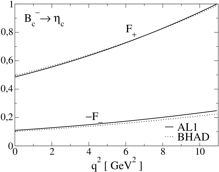
Figure 4.1: $F_{+}$ and $F_{-}$ form factors for $B_{c}^{-}\to\eta_{c}$ and $B_{c}^{-}\to\chi_{c0}$ semileptonic decays evaluated with the AL1 potential. In the first case, and for comparison, we also show with dotted lines the results obtained with the Bhaduri (BHAD) potential.

In Fig. 4.1 we show our results for the $F_{+}$ and $F_{-}$ form factors for the semileptonic $B_{c}^{-}\to\eta_{c},\,\chi_{c0}$ transitions. The minimum $q^{2}$ value depends on the actual final lepton and it is given, neglecting neutrino masses, by the lepton mass as $q^{2}_{min}=m_{l}^{2}$. The form factors have been evaluated using the AL1 potential. For decays into $\eta_{c}$, and for the sake of comparison, we also show the results obtained using the BHAD potential. As seen in the figures the differences between the form factors evaluated with the two inter-quark interactions are smaller than 10%.

In Table 4.3 we show $F_{+}$ and $F_{-}$ evaluated at $q^{2}_{\mathrm{min}}$ and $q^{2}_{\mathrm{max}}$ for a final light lepton ($l=e,\,\mu$) and compare them to the ones obtained by Ivanov et al. in Ref. [163], and, when available, by Ebert et al. in Ref. [165]. For the $B_{c}\to\eta_{c}$ transition we also show the corresponding values for the $F_{0}$ form factor defined as

$$F_{0}(q^{2})=F_{+}(q^{2})+\frac{q^{2}}{m^{2}_{B_{c}}-m^{2}_{\eta_{c}}}\ F_{-}(q^{2})$$ (4.11)

Our results for the $\eta_{c}$ case are in excellent agreement with the ones obtained by Ebert et al.. Compared to the results by Ivanov et al. we find large discrepancies for $F_{-}$.

$B_{c}^{-}\to\eta_{c}\,l^{-}\bar{\nu}_{l}\ \$	$q^{2}_{\mathrm{min}}$	$q^{2}_{\mathrm{max}}$	$B_{c}^{-}\to\chi_{c0}\,l^{-}\bar{\nu}_{l}\ \$	$q^{2}_{\mathrm{min}}$	$q^{2}_{\mathrm{max}}$
$F_{+}$			$F_{+}$
This work	$0.49^{+0.01}$	$1.00_{-0.01}$	This work	$0.30^{+0.01}$	$0.64^{+0.01}_{-0.01}$
[163]	0.61	1.14	[163]	0.40	0.65
[165]	0.47	1.07
$F_{-}$			$F_{-}$
This work	$-0.11^{+0.01}_{-0.01}$	$-0.25^{+0.03}$	This work	$-0.62^{+0.01}_{-0.03}$	$-1.35^{+0.05}$
[163]	$-0.32$	$-0.61$	[163]	$-1.00$	$-1.63$
$F_{0}$
This work	$0.49^{+0.01}$	$0.91^{+0.01}$
[165]	0.47	0.92

Table 4.3: $F_{+}$ and $F_{-}$ evaluated at $q^{2}_{\mathrm{min}}$ and $q^{2}_{\mathrm{max}}$ compared to the ones obtained by Ivanov et al. [163] and Ebert et al. Ref. [165]. Our central values have been obtained with the AL1 potential. For the $\eta_{c}$ channel we also show $F_{0}$ (see text for definition). Here $l$ stands for $l=e,\,\mu$.

$\bullet$ $B_{c}^{-}\to J/\Psi\,l\,\bar{\nu}_{l},\ h_{c}\,l\,\bar{\nu}_{l},\ \chi_{c1}\,l\,\bar{\nu}_{l}$ decays

Let us now see the form factors for the semileptonic $B_{c}^{-}$ decays into vector $J/\Psi$ and axial vector $h_{c}$ ($S_{q\bar{q}}=0$) and $\chi_{c1}$ ($S_{q\bar{q}}=1$) $c\bar{c}$ mesons. For the decay into $J/\Psi$ the form factors can be evaluated in terms of matrix elements as:

$$V(q^{2}) = \frac{i}{\sqrt{2}}\,\frac{m_{B_{c}}+m_{J/\Psi}}{m_{B_{c}}\,|\vec{q}\,|}\ V^{1}_{\lambda=-1}(|\vec{q}\,|)$$

$$A_{+}(q^{2}) = i\,\frac{m_{B_{c}}+m_{J/\Psi}}{2m_{B_{c}}}\,\frac{m_{J/\Psi}}{|\vec{q}\,|\,m_{B_{c}}}\,\bigg{\{}-A^{0}_{\lambda=0}(|\vec{q}\,|)+\frac{m_{B_{c}}-E_{J/\Psi}(-\vec{q}\,)}{|\vec{q}\,|}\,A^{3}_{\lambda=0}(|\vec{q}\,|)$$

$$\hskip 113.81102pt-\sqrt{2}\,\frac{m_{B_{c}}E_{J/\Psi}(-\vec{q}\,)-m^{2}_{J/\Psi}}{|\vec{q}\,|\,m_{J/\Psi}}\,A^{1}_{\lambda=-1}(|\vec{q}\,|)\bigg{\}}$$

$$A_{-}(q^{2}) = -i\,\frac{m_{B_{c}}+m_{J/\Psi}}{2m_{B_{c}}}\,\frac{m_{J/\Psi}}{|\vec{q}\,|\,m_{B_{c}}}\,\bigg{\{}\ A^{0}_{\lambda=0}(|\vec{q}\,|)+\frac{m_{B_{c}}+E_{J/\Psi}(-\vec{q}\,)}{|\vec{q}\,|}\,A^{3}_{\lambda=0}(|\vec{q}\,|)$$

$$\hskip 113.81102pt-\sqrt{2}\,\frac{m_{B_{c}}E_{J/\Psi}(-\vec{q}\,)+m^{2}_{J/\Psi}}{|\vec{q}\,|\,m_{J/\Psi}}\,A^{1}_{\lambda=-1}(|\vec{q}\,|)\bigg{\}}$$

$$A_{0}(q^{2}) = -i\sqrt{2}\,\frac{1}{m_{B_{c}}-m_{J/\Psi}}\,A^{1}_{\lambda=-1}(|\vec{q}\,|)$$ (4.12)

with $V^{\mu}_{\lambda}(|\vec{q}\,|)$ and $A^{\mu}_{\lambda}(|\vec{q}\,|)$ calculated in our model as

$$V^{\mu}_{\lambda}(|\vec{q}\,|) = \left\langle\,J/\Psi,\hskip 5.69046pt\lambda\ -|\vec{q}\,|\,\vec{k}\,\left|\,J^{c\,b\ \mu}_{V}(0)\,\right|\,B_{c}^{-},\,\vec{0}\right\rangle$$

$$= \sqrt{2m_{B_{c}}2E_{J/\Psi}(-\vec{q}\,)}\ \ {}_{\stackrel{{\scriptstyle}}{{\stackrel{{\scriptstyle}}{{NR}}}}}\left\langle\,J/\Psi,\hskip 5.69046pt\lambda\,-|\vec{q}\,|\,{\vec{k}}\,\left|\,J^{c\,b\ \mu}_{V}(0)\,\right|\,B_{c}^{-},\,\vec{0}\right\rangle_{NR}$$

$$A^{\mu}_{\lambda}(|\vec{q}\,|) = \left\langle\,J/\Psi,\hskip 5.69046pt\lambda\ -|\vec{q}\,|\,\vec{k}\,\left|\,J^{c\,b\ \mu}_{A}(0)\,\right|\,B_{c}^{-},\,\vec{0}\right\rangle$$

$$= \sqrt{2m_{B_{c}}2E_{J/\Psi}(-\vec{q}\,)}\ \ {}_{\stackrel{{\scriptstyle}}{{\stackrel{{\scriptstyle}}{{NR}}}}}\left\langle\,J/\Psi,\hskip 5.69046pt\lambda\,-|\vec{q}\,|\,{\vec{k}}\,\left|\,J^{c\,b\ \mu}_{A}(0)\,\right|\,B_{c}^{-},\,\vec{0}\right\rangle_{NR}$$

which expressions are given in appendix E.

The form factors corresponding to transitions to the $\chi_{c1}$ and $h_{c}$ axial vector mesons are obtained from the expressions in Eq.(4.3.1) by just changing

$$V^{\mu}_{\lambda}(|\vec{q}\,|)\longleftrightarrow-A^{\mu}_{\lambda}(|\vec{q}\,|)$$ (4.14)

and using the appropriate mass for the final meson. Obviously in Eq. (4.3.1) $J/\Psi$ has to be replaced by $\chi_{c_{1}}$ or $h_{c}$.

In Table 4.4 we show the results for the different form factors evaluated at $q^{2}_{\mathrm{min}}$ and $q^{2}_{\mathrm{max}}$ for the case where the final lepton is light ($l=e,\,\mu$). For the decay into $J/\Psi$ we also show the combination of form factors:

$$\widetilde{A}_{0}(q^{2})=\frac{m_{B_{c}}-m_{J/\Psi}}{2m_{J/\Psi}}\left(A_{0}(q^{2})-A_{+}(q^{2})\right)-\frac{q^{2}}{2m_{J/\Psi}\,(m_{B_{c}}+m_{J/\Psi})}\ A_{-}(q^{2})$$ (4.15)

Our results for the $B_{c}\to J/\Psi$ decay channel are in agreement with the ones obtained by Ebert et al.. They also agree reasonably well, with the exception of $A_{-}$, with the ones obtained by Ivanov et al.. For the other two cases the discrepancies are in general large.

$B_{c}^{-}\to J/\Psi\,l^{-}\bar{\nu}_{l}\ \$	$q^{2}_{\mathrm{min}}$	$q^{2}_{\mathrm{max}}$	$B_{c}^{-}\to h_{c}\,l^{-}\bar{\nu}_{l}\ \$	$q^{2}_{\mathrm{min}}$	$q^{2}_{\mathrm{max}}$
$V$			$V$
This work	$-0.61_{-0.03}$	$-1.26^{+0.01}$	This work	$-0.040_{-0.003}$	$-0.078_{-0.003}$
[163]	$-0.83$∗	$-1.53$∗	[163]	$-0.25$ ∗	$-0.365$∗
[165]	$-0.49$	$-1.34$
$A_{+}$			$A_{+}$
This work	$0.56^{+0.03}$	$1.13^{+0.01}$	This work	$-0.85^{+0.01}_{-0.05}$	$-1.90^{+0.06}$
[163]	0.54	0.97	[163]	$-1.08$	$-1.80$
[165]	0.73	1.33
$A_{-}$			$A_{-}$
This work	$-0.60_{-0.03}$	$-1.24_{-0.01}$	This work	$0.12^{+0.01}_{-0.02}$	$0.36_{-0.06}$
[163]	$-0.95$	$-1.76$	[163]	0.52	0.89
$A_{0}$			$A_{0}$
This work	$1.44^{+0.08}$	$2.58^{+0.01}_{-0.02}$	This work	$0.28^{+0.02}$	$0.52^{+0.02}$
[163]	1.64	2.50	[163]	0.44	0.54
[165]	1.47	2.59
$\widetilde{A}_{0}$
This work	$0.45^{+0.03}$	$0.96_{-0.01}$
[165]	0.40	1.06
$B_{c}^{-}\to\chi_{c1}\,l^{-}\bar{\nu}_{l}\ \$	$q^{2}_{\mathrm{min}}$	$q^{2}_{\mathrm{max}}$
$V$
This work	$0.92^{+0.04}_{-0.02}$	$1.86_{-0.12}$
[163]	1.18∗	1.81∗
$A_{+}$
This work	$-0.44_{-0.03}$	$-0.78^{+0.04}$
[163]	$-0.39$	$-0.50$
$A_{-}$
This work	$0.96^{+0.04}_{-0.01}$	$1.97_{-0.13}$
[163]	1.52	2.36
$A_{0}$
This work	$-0.50_{-0.02}$	$-0.32_{-0.02}$
[163]	$-0.064$	0.46

Table 4.4: $V$, $A_{+}$, $A_{-}$ and $A_{0}$ form factors evaluated at $q^{2}_{\mathrm{min}}$ and $q^{2}_{\mathrm{max}}$ compared to the ones obtained by Ivanov et al. [163] and Ebert et al. Ref. [165]. Our central values have been evaluated with the AL1 potential. For the $J/\Psi$ channel we also show $\widetilde{A}_{0}$ (see text for definition). Here $l$ stands for $l=e,\,\mu$. The asterisk to the right of a number means we have changed its sign to account for the different choice of $\varepsilon^{\,0\,1\,2\,3}$ in Ref. [163].

All the form factors are depicted in Figs. 4.2 and 4.3

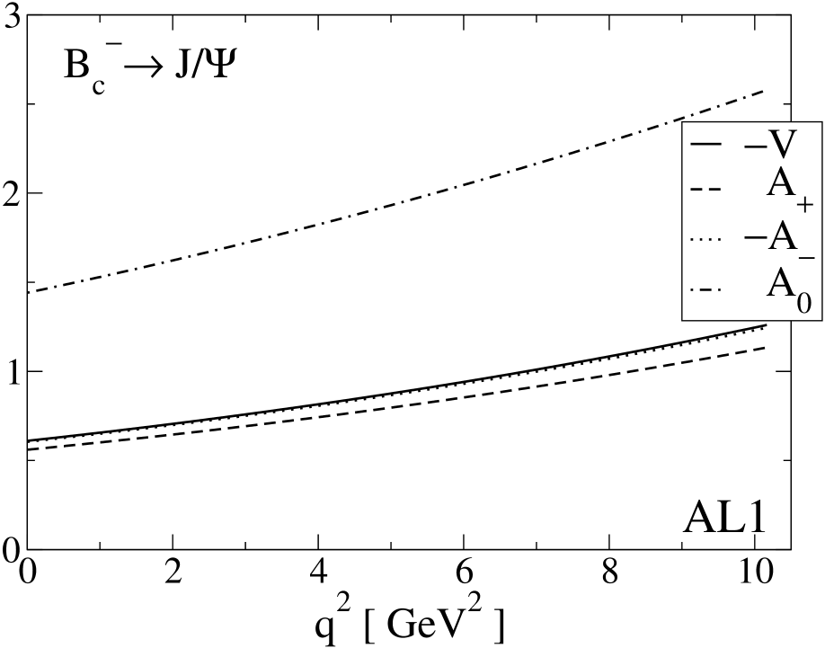
Figure 4.2: $V$ (solid line), $A_{+}$ (dashed line), $A_{-}$ (dotted line) and $A_{0}$ (dashed-dotted line) form factors for the $B_{c}^{-}\to J/\Psi$ semileptonic decays evaluated with the AL1 potential.

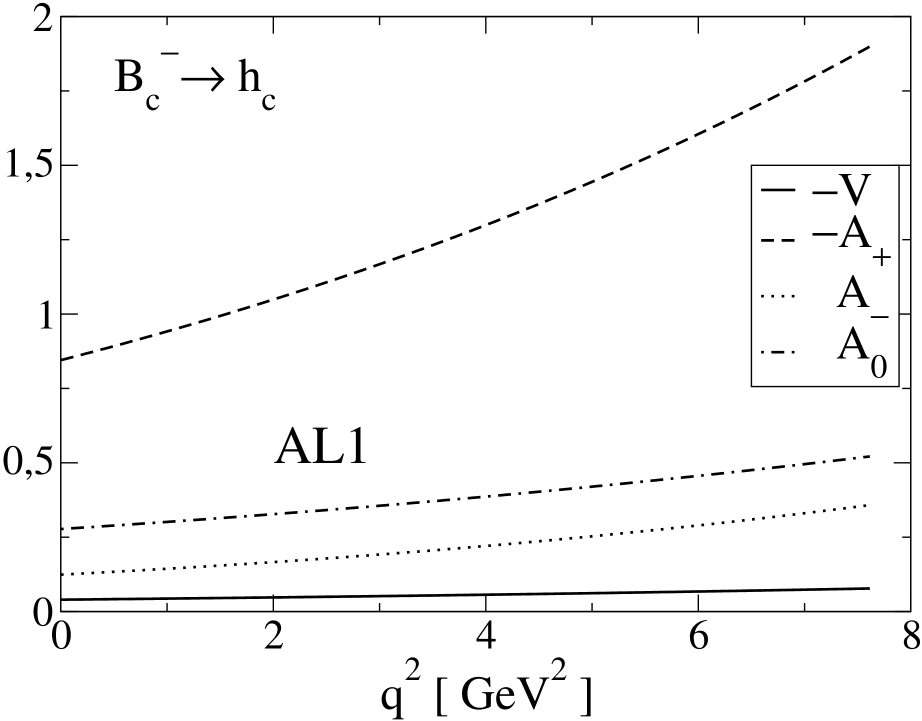
Figure 4.3: $V$ (solid line), $A_{+}$ (dashed line), $A_{-}$ (dotted line) and $A_{0}$ (dashed-dotted line) form factors for $B_{c}^{-}\to h_{c}$ and $B_{c}^{-}\to\chi_{c1}$ semileptonic decays evaluated with the AL1 potential.

$\bullet$$B_{c}^{-}\to\Psi(3836)\,l\,\bar{\nu}_{l},\ \chi_{c2}\,l\,\bar{\nu}_{l}$, decays

Finally let us see the form factors for the $B_{c}^{-}$ decays into tensor $\chi_{c2}$ and pseudotensor $\Psi(3836)$  mesons. For the decay into $\chi_{c2}$ the form factors can be evaluated in terms of matrix elements as:

$$T_{1}(q^{2}) = -i\,\frac{2m_{\chi_{c2}}}{m_{B_{c}}|\vec{q}\,|}\ A^{1}_{T\lambda=+1}(|\vec{q}\,|)$$

$$T_{2}(q^{2}) = i\,\frac{1}{2m^{3}_{B_{c}}}\,\bigg{\{}-\sqrt{\frac{3}{2}}\,\frac{m^{2}_{\chi_{c2}}}{|\vec{q}\,|^{2}}\,A^{0}_{T\lambda=0}(|\vec{q}\,|)-\sqrt{\frac{3}{2}}\,\frac{m^{2}_{\chi_{c2}}}{|\vec{q}\,|^{3}}\,\left(E_{\chi_{c2}}(-\vec{q}\,)-m_{B_{c}}\right)A^{3}_{T\lambda=0}(|\vec{q}\,|)$$

$$\hskip 44.10185pt+\frac{2m_{\chi_{c2}}}{|\vec{q}\,|}\left(1-\frac{E_{\chi_{c2}}(-\vec{q}\,)}{|\vec{q}\,|^{2}}\left(E_{\chi_{c2}}(-\vec{q}\,)-m_{B_{c}}\right)\right)\,A^{1}_{T\lambda=+1}(|\vec{q}\,|)\bigg{\}}$$

$$T_{3}(q^{2}) = i\,\frac{1}{2m^{3}_{B_{c}}}\,\bigg{\{}-\sqrt{\frac{3}{2}}\,\frac{m^{2}_{\chi_{c2}}}{|\vec{q}\,|^{2}}\,A^{0}_{T\lambda=0}(|\vec{q}\,|)-\sqrt{\frac{3}{2}}\,\frac{m^{2}_{\chi_{c2}}}{|\vec{q}\,|^{3}}\,\left(E_{\chi_{c2}}(-\vec{q}\,)+m_{B_{c}}\right)A^{3}_{T\lambda=0}(|\vec{q}\,|)$$

$$\hskip 41.25641pt+\frac{2m_{\chi_{c2}}}{|\vec{q}\,|}\left(1-\frac{E_{\chi_{c2}}(-\vec{q}\,)}{|\vec{q}\,|^{2}}\left(E_{\chi_{c2}}(-\vec{q}\,)+m_{B_{c}}\right)\right)\,A^{1}_{T\lambda=+1}(|\vec{q}\,|)\bigg{\}}$$

$$T_{4}(q^{2}) = i\,\frac{m_{\chi_{c2}}}{m^{2}_{B_{c}}|\vec{q}\,|^{2}}\,V^{1}_{T\lambda=+1}(|\vec{q}\,|)$$ (4.16)

with $V^{\mu}_{T\lambda}(|\vec{q}\,|)$ and $A^{\mu}_{T\lambda}(|\vec{q}\,|)$ calculated in our model as

$$V^{\mu}_{T\lambda}(|\vec{q}\,|) = \left\langle\,\chi_{c2},\hskip 5.69046pt\lambda\ -|\vec{q}\,|\,\vec{k}\,\left|\,J^{c\,b\ \mu}_{V}(0)\,\right|\,B_{c}^{-},\,\vec{0}\right\rangle$$

$$= \sqrt{2m_{B_{c}}2E_{\chi_{c2}}(-\vec{q}\,)}\ \ {}_{\stackrel{{\scriptstyle}}{{\stackrel{{\scriptstyle}}{{NR}}}}}\left\langle\,\chi_{c2},\hskip 5.69046pt\lambda\,-|\vec{q}\,|\,{\vec{k}}\,\left|\,J^{c\,b\ \mu}_{V}(0)\,\right|\,B_{c}^{-},\,\vec{0}\right\rangle_{NR}$$

$$A^{\mu}_{T\lambda}(|\vec{q}\,|) = \left\langle\,\chi_{c2},\hskip 5.69046pt\lambda\ -|\vec{q}\,|\,\vec{k}\,\left|\,J^{c\,b\ \mu}_{A}(0)\,\right|\,B_{c}^{-},\,\vec{0}\right\rangle$$

$$= \sqrt{2m_{B_{c}}2E_{\chi_{c2}}(-\vec{q}\,)}\ \ {}_{\stackrel{{\scriptstyle}}{{\stackrel{{\scriptstyle}}{{NR}}}}}\left\langle\,\chi_{c2},\hskip 5.69046pt\lambda\,-|\vec{q}\,|\,{\vec{k}}\,\left|\,J^{c\,b\ \mu}_{A}(0)\,\right|\,B_{c}^{-},\,\vec{0}\right\rangle_{NR}$$

which expressions are given in appendix E.

The form factors corresponding to transitions to $\Psi(3836)$ are obtained from the expressions in Eq.(4.3.1) by just changing

$$V^{\mu}_{T\lambda}(|\vec{q}\,|)\longleftrightarrow-A^{\mu}_{T\lambda}(|\vec{q}\,|)$$ (4.18)

and using the appropriate mass for the final meson. Besides in Eq. (4.3.1) $\chi_{c_{2}}$ has to be replaced by $\Psi(3836)$.

The results for the different form factors appear in Fig. 4.4.

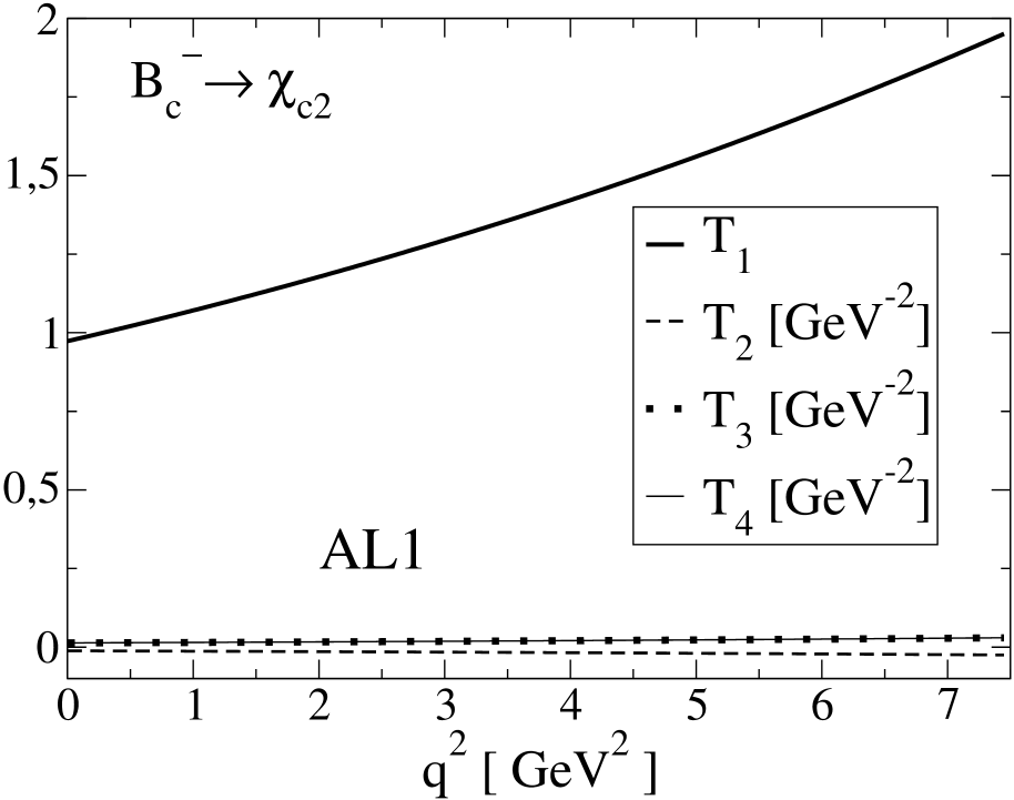
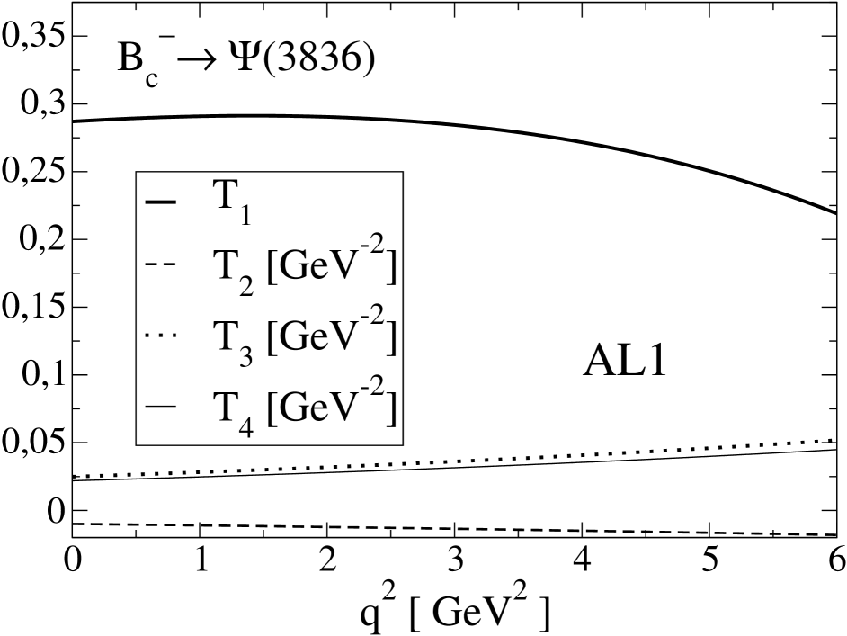
Figure 4.4: $T_{1}$ (bold solid line), $T_{2}$ (dashed line), $T_{3}$ (dotted line) and $T_{4}$ (thin solid line) form factors for $B_{c}^{-}\to\chi_{c2}$ and $B_{c}^{-}\to\Psi(3836)$ semileptonic decays evaluated with the AL1 potential.

In Table 4.5 we show $T_{1}$, $T_{2}$, $T_{3}$ and $T_{4}$ evaluated at $q^{2}_{min}$ and $q^{2}_{max}$ for the case of a final light lepton, and compare them to the values obtained by Ivanov et al. [163]. For the $B_{c}^{-}\to\chi_{c2}$ transition we find a reasonable agreement between the two calculations. For $B_{c}^{-}\to\Psi(3836)$ there is also a reasonable agreement for the absolute values of the form factors but we disagree for some of the signs.

$B_{c}^{-}\to\chi_{c2}\,l^{-}\bar{\nu}_{l}\ \$	$q^{2}_{\mathrm{min}}$	$q^{2}_{\mathrm{max}}$	$B_{c}^{-}\to\Psi(3836)\,l^{-}\bar{\nu}_{l}\ \$	$q^{2}_{\mathrm{min}}$	$q^{2}_{\mathrm{max}}$
$T_{1}$			$T_{1}$
This work	$0.97^{+0.08}_{-0.01}$	$1.95_{-0.06}$	This work	$0.29_{-0.02}$	$0.22_{-0.01}$
[163]	1.22	1.69	[163]	0.052	0.35
$T_{2}\ [GeV^{-2}]$			$T_{2}\ [GeV^{-2}]$
This work	$-0.012_{-0.001}$	$-0.025^{+0.001}$	This work	$-0.010^{+0.006}$	$-0.018^{+0.001}$
[163]	$-0.011$	$-0.018$	[163]	0.0071	0.0090
$T_{3}\ [GeV^{-2}]$			$T_{3}\ [GeV^{-2}]$
This work	$0.013^{+0.001}$	$0.030_{-0.001}$	This work	$0.025_{-0.002}$	$0.052_{-0.004}$
[163]	0.025	0.040	[163]	$-0.036$	$-0.052$
$T_{4}\ [GeV^{-2}]$			$T_{4}\ [GeV^{-2}]$
This work	$0.013^{+0.001}$	$0.030_{-0.001}$	This work	$0.022_{-0.001}$	$0.045_{-0.003}$
[163]	0.021∗	0.033∗	[163]	$-0.026$∗	$-0.038$∗

Table 4.5: Values for $T_{1}$, $T_{2}$, $T_{3}$ and $T_{4}$ evaluated at $q^{2}_{\mathrm{min}}$ and $q^{2}_{\mathrm{max}}$ compared to the ones obtained by Ivanov et al. [163]. Here $l$ stands for $l=e,\,\mu$. Asterisk as in Table 4.4.

4.3.2 Decay width

For a $B_{c}$ at rest the double differential decay width with respect to $q^{2}$ and $x_{l}$, being $x_{l}$ the cosine of the angle between the final meson momentum and the momentum of the final charged lepton measured in the lepton–neutrino center of mass frame (CMF), is given by

$$\frac{d^{2}\Gamma}{dq^{2}dx_{l}}=\frac{G_{F}^{2}}{64m^{2}_{B_{c}}}\,\frac{|V_{bc}|^{2}}{8\pi^{3}}\,\frac{\lambda^{1/2}(q^{2},m^{2}_{B_{c}},m^{2}_{c\bar{c}})}{2m_{B_{c}}}\,\frac{q^{2}-m^{2}_{l}}{q^{2}}\ {\cal H}_{\alpha\,\beta}({P}_{B_{c}},{P}_{c\bar{c}})\ {\cal L}^{\alpha\,\beta}({p}_{l},{p}_{{\nu}})$$

where $\lambda(a,b,c)=(a+b-c)^{2}-4ab$, $m_{l}$ is the mass of the charged lepton, ${\cal H}_{\alpha\,\beta}$ and ${\cal L}^{\alpha\,\beta}$ are the hadron and lepton tensors, and ${P}_{B_{c}},\ {P}_{c\bar{c}},\ {p}_{l},\ {p}_{{\nu}}$ are the meson and lepton four–momenta. The lepton tensor is

$${\cal L}^{\alpha\,\beta}({p}_{l},{p}_{{\nu}})=8\left({p}_{l}^{\alpha}{p}_{{\nu}}^{\beta}+{p}_{l}^{\beta}{p}_{{\nu}}^{\alpha}-g^{\alpha\beta}{p}_{l}\cdot{p}_{{\nu}}\mp i\,\varepsilon^{\alpha\,\beta\,\sigma\,\rho}p_{l\,\sigma}p_{\nu\,\rho}\right)$$ (4.20)

As for the hadron tensor it is given by

$${\cal H}_{\alpha\,\beta}({P}_{B_{c}},{P}_{c\bar{c}}) = \sum_{\lambda}\ h_{(\lambda)\,\alpha}({P}_{B_{c}},{P}_{c\bar{c}})\,h^{*}_{(\lambda)\,\beta}({P}_{B_{c}},{P}_{c\bar{c}})$$ (4.21)

with

$$h_{(\lambda)\,\alpha}({P}_{B_{c}},{P}_{c\bar{c}})=\left\langle c\bar{c},\,\lambda\,\vec{P}_{c\bar{c}}|J_{\alpha}^{cb}(0)|B_{c},\,\vec{P}_{B_{c}}\right\rangle$$ (4.22)

The quantity

$${\cal H}_{\alpha\,\beta}({P}_{B_{c}},{P}_{c\bar{c}})\ {\cal L}^{\alpha\,\beta}({p}_{l},{p}_{\nu})$$ (4.23)

is a scalar and to evaluate it we can choose $\vec{P}_{c\bar{c}}$ along the negative $z$-axis. This implies also that the CMF of the final leptons moves in the positive $z$-direction. Furthermore we shall follow Ref. [163] and introduce helicity components for the hadron and lepton tensors. For that purpose we rewrite

$${\cal H}_{\alpha\,\beta}({P}_{B_{c}},{P}_{c\bar{c}})\ {\cal L}^{\alpha\,\beta}({p}_{l},{p}_{\nu})={\cal H}^{\sigma\,\rho}({P}_{B_{c}},{P}_{c\bar{c}})\ g_{\sigma\alpha}\,g_{\rho\beta}\ {\cal L}^{\alpha\,\beta}({p}_{l},{p}_{\nu})$$ (4.24)

and use [189]

$$g_{\mu\nu}=\sum_{r=t,\pm 1,0}\ g_{rr}\ \varepsilon_{(r)\,\mu}({q})\,\varepsilon_{(r)\,\nu}^{*}({q})\hskip 14.22636pt;\hskip 14.22636ptg_{tt}=1,g_{\pm 1,0}=-1$$ (4.25)

with $\varepsilon^{\mu}_{(t)}({q})=q^{\mu}/q^{2}$ and where the $\varepsilon_{(r)}({q}),\,r=\pm 1,\,0$ are the polarization vectors for an on–shell vector particle with four–momentum ${q}$ and helicity $r$. Defining helicity components for the hadron and lepton tensors as

$${\cal H}_{r\,s}({P}_{B_{c}},{P}_{c\bar{c}}) = \varepsilon_{(r)\,\sigma}^{*}({q})\,{\cal H}^{\sigma\,\rho}({P}_{B_{c}},{P}_{c\bar{c}})\,\varepsilon_{(s)\,\rho}({q})$$

$${\cal L}_{r\,s}({p}_{l},{p}_{\nu}) = \varepsilon_{(r)\,\alpha}({q})\,{\cal L}^{\alpha\,\beta}({p}_{l},{p}_{\nu})\,\varepsilon_{(s)\,\beta}^{*}({q})$$ (4.26)

we have that

$${\cal H}_{\alpha\,\beta}({P}_{B_{c}},{P}_{c\bar{c}})\ {\cal L}^{\alpha\,\beta}({p}_{l},{p}_{\nu})=\sum_{r=t,\pm 1,0}\sum_{s=t,\pm 1,0}\ g_{rr}\,g_{ss}\ {\cal H}_{r\,s}({P}_{B_{c}},{P}_{c\bar{c}})\ {\cal L}_{r\,s}({p}_{l},{p}_{\nu})$$

Let us start with the lepton tensor. We can take advantage of the fact that the Wigner rotation relating the original frame and the CMF of the final leptons is the identity to evaluate the lepton tensor helicity components in this latter reference system

$${\cal L}_{r\,s}({p}_{l},{p}_{\nu}) = \varepsilon_{(r)\,\alpha}({q})\,{\cal L}^{\alpha\,\beta}({p}_{l},{p}_{\nu})\,\varepsilon_{(s)\,\beta}^{*}({q})=\varepsilon_{(r)\,\alpha}(\widetilde{q})\,{\cal L}^{\alpha,\beta}(\widetilde{p}_{l},\widetilde{p}_{\nu})\,\varepsilon_{(s)\,\beta}^{*}(\widetilde{q})$$

were the tilde stands for momenta measured in the final leptons CMF. For the purpose of evaluation we can use

$$\widetilde{p}_{l}^{\alpha} = (E_{l}(|\widetilde{p}_{l}|),-|\widetilde{p}_{l}|\,\sqrt{1-x_{l}^{2}},0,-|\widetilde{p}_{l}|\,x_{l})$$

$$\widetilde{p}_{\nu}^{\alpha} = (|\widetilde{p}_{l}|,|\widetilde{p}_{l}|\,\sqrt{1-x_{l}^{2}},0,|\widetilde{p}_{l}|\,x_{l})$$ (4.29)

with $|\widetilde{p}_{l}|$ the modulus of the lepton three-momentum measured in the leptons CMF.

The only helicity components that we shall need are the following.

$${\cal L}_{t\,t}({p}_{l},{p}_{\nu}) = 4\frac{m_{l}^{2}(q^{2}-m_{l}^{2})}{q^{2}}$$

$${\cal L}_{t\,0}({p}_{l},{p}_{\nu}) = {\cal L}_{0\,t}({p}_{l},{p}_{\nu})=-4x_{l}\frac{m_{l}^{2}(q^{2}-m_{l}^{2})}{q^{2}}$$

$${\cal L}_{+1\,+1}({p}_{l},{p}_{\nu}) = (q^{2}-m_{l}^{2})\,\left(4(1\pm x_{l})-2(1-x_{l}^{2})\frac{q^{2}-m_{l}^{2}}{q^{2}}\right)$$

$${\cal L}_{-1\,-1}({p}_{l},{p}_{\nu}) = (q^{2}-m_{l}^{2})\,\left(4(1\mp x_{l})-2(1-x_{l}^{2})\frac{q^{2}-m_{l}^{2}}{q^{2}}\right)$$

$${\cal L}_{0\,0}({p}_{l},{p}_{\nu}) = 4(q^{2}-m_{l}^{2})\,\left(1-x_{l}^{2}\frac{q^{2}-m_{l}^{2}}{q^{2}}\right)$$

As for the hadron tensor it is convenient to introduce helicity amplitudes defined as

$$h_{(\lambda)\,r}({P}_{B_{c}},{P}_{c\bar{c}})=\varepsilon_{(r)\,\alpha}^{*}({q})\ h_{(\lambda)}^{\alpha}({P}_{B_{c}},{P}_{c\bar{c}})\hskip 14.22636pt,\hskip 14.22636ptr=t,\,\pm 1,\,0$$ (4.31)

in terms of which

$${\cal H}_{r\,s}({P}_{B_{c}},{P}_{c\bar{c}})=\sum_{\lambda}h_{(\lambda)\,r}({P}_{B_{c}},{P}_{c\bar{c}})\,h_{(\lambda)\,s}^{*}({P}_{B_{c}},{P}_{c\bar{c}})$$ (4.32)

We now give the expressions for the helicity amplitudes evaluated in the original frame.

• Case $0^{-}\to 0^{-},0^{+}$.

  $$h_{t}({P}_{B_{c}},{P}_{c\bar{c}}) = \frac{m^{2}_{B_{c}}-m^{2}_{c\bar{c}}}{\sqrt{q^{2}}}\,F_{+}(q^{2})+\sqrt{q^{2}}\,F_{-}(q^{2})$$

  $$h_{0}({P}_{B_{c}},{P}_{c\bar{c}}) = \frac{\lambda^{1/2}(q^{2},m^{2}_{B_{c}},m^{2}_{c\bar{c}})}{\sqrt{q^{2}}}\,F_{+}(q^{2})$$

  $$h_{+1}({P}_{B_{c}},{P}_{c\bar{c}}) = h_{-1}({P}_{B_{c}},{P}_{c\bar{c}})=0$$ (4.33)

• Case $0^{-}\to 1^{-},1^{+}$.

  $$h_{(\lambda)\,t}({P}_{B_{c}},{P}_{c\bar{c}}) = i\delta_{\lambda\,0}\,\frac{\lambda^{1/2}(q^{2},m^{2}_{B_{c}},m^{2}_{c\bar{c}})}{2m_{c\bar{c}}\sqrt{q^{2}}}\,$$

  $$\hskip 2.84544pt\left((m_{B_{c}}-m_{c\bar{c}})\left(A_{0}(q^{2})-A_{+}(q^{2})\right)-\frac{q^{2}}{m_{B_{c}}+m_{c\bar{c}}}A_{-}(q^{2})\right)$$

  $$h_{(\lambda)\,+1}({P}_{B_{c}},{P}_{c\bar{c}}) = -i\delta_{\lambda\,-1}\,\left(\ \frac{\lambda^{1/2}(q^{2},m^{2}_{B_{c}},m^{2}_{c\bar{c}})}{m_{B_{c}}+m_{c\bar{c}}}\,V(q^{2})+(m_{B_{c}}-m_{c\bar{c}})\,A_{0}(q^{2})\right)$$

  $$h_{(\lambda)\,-1}({P}_{B_{c}},{P}_{c\bar{c}}) = -i\delta_{\lambda\,+1}\,\left(-\frac{\lambda^{1/2}(q^{2},m^{2}_{B_{c}},m^{2}_{c\bar{c}})}{m_{B_{c}}+m_{c\bar{c}}}\,V(q^{2})+(m_{B_{c}}-m_{c\bar{c}})\,A_{0}(q^{2})\right)$$

  $$h_{(\lambda)\,0}({P}_{B_{c}},{P}_{c\bar{c}}) = i\delta_{\lambda\,0}\,\left((m_{B_{c}}-m_{c\bar{c}})\frac{m^{2}_{B_{c}}-q^{2}-m^{2}_{c\bar{c}}}{2m_{c\bar{c}}\sqrt{q^{2}}}\,A_{0}(q^{2})\right.$$ (4.34)

  $$\hskip 56.9055pt\left.-\frac{\lambda(q^{2},m^{2}_{B_{c}},m^{2}_{c\bar{c}})}{2m_{c\bar{c}}\sqrt{q^{2}}}\,\frac{A_{+}(q^{2})}{m_{B_{c}}+m_{c\bar{c}}}\right)$$

• Case $0^{-}\to 2^{-},2^{+}$.

  $$h_{(\lambda)\,t}({P}_{B_{c}},{P}_{c\bar{c}}) = -i\delta_{\lambda\,0}\,\sqrt{\frac{2}{3}}\ \frac{\lambda(q^{2},m^{2}_{B_{c}},m^{2}_{c\bar{c}})}{4\,m^{2}_{c\bar{c}}\,\sqrt{q^{2}}}\,$$

  $$\hskip 28.45274pt\left(\,T_{1}(q^{2})+(m^{2}_{B_{c}}-m^{2}_{c\bar{c}})\,T_{2}(q^{2})+q^{2}\,T_{3}(q^{2})\,\right)$$

  $$h_{(\lambda)\,+1}({P}_{B_{c}},{P}_{c\bar{c}}) = i\delta_{\lambda\,-1}\,\frac{1}{\sqrt{2}}\,\frac{\lambda^{1/2}(q^{2},m^{2}_{B_{c}},m^{2}_{c\bar{c}})}{2\,m_{c\bar{c}}}\,$$

  $$\hskip 28.45274pt\left(\,T_{1}(q^{2})-\lambda^{1/2}(q^{2},m^{2}_{B_{c}},m^{2}_{c\bar{c}})\,T_{4}(q^{2})\,\right)$$

  $$h_{(\lambda)\,-1}({P}_{B_{c}},{P}_{c\bar{c}}) = i\delta_{\lambda\,+1}\,\frac{1}{\sqrt{2}}\,\frac{\lambda^{1/2}(q^{2},m^{2}_{B_{c}},m^{2}_{c\bar{c}})}{2\,m_{c\bar{c}}}\,$$

  $$\hskip 28.45274pt\left(\,T_{1}(q^{2})+\lambda^{1/2}(q^{2},m^{2}_{B_{c}},m^{2}_{c\bar{c}})\,T_{4}(q^{2})\,\right)$$

  $$h_{(\lambda)\,0}({P}_{B_{c}},{P}_{c\bar{c}}) = -i\delta_{\lambda\,0}\,\sqrt{\frac{2}{3}}\ \frac{\lambda^{1/2}(q^{2},m^{2}_{B_{c}},m^{2}_{c\bar{c}})}{4\,m^{2}_{c\bar{c}}\,\sqrt{q^{2}}}\,$$

  $$\hskip 28.45274pt\left(\,(m^{2}_{B_{c}}-q^{2}-m^{2}_{c\bar{c}})\,T_{1}(q^{2})+\lambda(q^{2},m^{2}_{B_{c}},m^{2}_{c\bar{c}})\,T_{2}(q^{2})\,\right)$$

We see that the helicity amplitudes, and thus the helicity components of the hadron tensor, only depend on $q^{2}$. The expressions for the latter are collected in appendix F.

We can now define the combinations [163]

$$H_{U} = {\cal H}_{+1\,+1}+{\cal H}_{-1\,-1}$$

$$H_{L} = {\cal H}_{0\,0}$$

$$H_{P} = {\cal H}_{+1\,+1}-{\cal H}_{-1\,-1}$$

$$H_{S} = 3\,{\cal H}_{t\,t}$$

$$H_{SL} = {\cal H}_{t\,0}$$

$$\widetilde{H}_{J} = \frac{m_{l}^{2}}{2\,q^{2}}\,H_{J}\hskip 14.22636pt;\hskip 14.22636ptJ=U,L,S,SL$$ (4.36)

with $U,\,L,\,P,\,S,\,SL$ representing respectively unpolarized–transverse, longitudinal, parity–odd, scalar and scalar–longitudinal interference.

Finally the double differential decay width is written in terms of the above defined combinations as

$$\frac{d^{2}\Gamma}{dq^{2}dx_{l}} = \frac{G_{F}^{2}}{8\pi^{3}}\,|V_{bc}|^{2}\,\frac{(q^{2}-m^{2}_{l})^{2}}{12m^{2}_{B_{c}}q^{2}}\,\frac{\lambda^{1/2}(q^{2},m^{2}_{B_{c}},m^{2}_{c\bar{c}})}{2m_{B_{c}}}\,$$ (4.37)

$$\hskip 14.22636pt\bigg{\{}\ \frac{3}{8}(1+x_{l}^{2})\,H_{U}+\frac{3}{4}(1-x_{l}^{2})\,H_{L}\pm\frac{3}{4}x_{l}H_{P}$$

$$\hskip 56.9055pt+\frac{3}{4}(1-x_{l}^{2})\widetilde{H}_{U}+\frac{3}{2}x^{2}_{l}\widetilde{H}_{L}+\frac{1}{2}\widetilde{H}_{S}+3x_{l}\widetilde{H}_{SL}\bigg{\}}$$

Note that for antiparticle decay $H_{P}$ has the opposite sign to the case of particle decay while all other hadron tensor helicity components combinations defined in Eq.(4.36) do not change (See appendix E.2 for details). The sign change of $H_{P}$ compensates the extra sign coming from the lepton tensor. This means that in fact the double differential decay width is the same for $B_{c}^{-}$ or $B_{c}^{+}$ decay.

Integrating over $x_{l}$ we obtain the differential decay width

$$\frac{d\Gamma}{dq^{2}} = \frac{G_{F}^{2}}{8\pi^{3}}\,|V_{bc}|^{2}\,\frac{(q^{2}-m^{2}_{l})^{2}}{12m^{2}_{B_{c}}q^{2}}\,\frac{\lambda^{1/2}(q^{2},m^{2}_{B_{c}},m^{2}_{c\bar{c}})}{2m_{B_{c}}}\,\bigg{\{}\ H_{U}+H_{L}+\widetilde{H}_{U}+\widetilde{H}_{L}+\widetilde{H}_{S}\bigg{\}}$$

from where, integrating over $q^{2}$, we obtain the total decay width that we write, following Ref. [163], as

$$\Gamma = \Gamma_{U}+\Gamma_{L}+\widetilde{\Gamma}_{U}+\widetilde{\Gamma}_{L}+\widetilde{\Gamma}_{S}$$ (4.39)

with $\Gamma_{J}$ and $\widetilde{\Gamma}_{J}$ partial helicity widths defined as

$$\Gamma_{J}=\int dq^{2}\frac{G_{F}^{2}}{8\pi^{3}}\,|V_{bc}|^{2}\,\frac{(q^{2}-m^{2}_{l})^{2}}{12m^{2}_{B_{c}}q^{2}}\,\frac{\lambda^{1/2}(q^{2},m^{2}_{B_{c}},m^{2}_{c\bar{c}})}{2m_{B_{c}}}\,H_{J}$$ (4.40)

and similarly for $\widetilde{\Gamma}_{J}$ in terms of $\widetilde{H}_{J}$.

$B^{-}_{c}\to$	$\Gamma_{U}$	$\widetilde{\Gamma}_{U}$	$\Gamma_{L}$	$\widetilde{\Gamma}_{L}$	$\Gamma_{P}$	$\widetilde{\Gamma}_{S}$	$\widetilde{\Gamma}_{SL}$
$\eta_{c}\,e^{-}\bar{\nu}_{e}$	0	0	$6.95^{+0.31}$	$0.13^{+0.01}\ 10^{-5}$	0	$0.44^{+0.03}\ 10^{-5}$	$0.14^{+0.01}\ 10^{-5}$
$\eta_{c}\,\mu^{-}\bar{\nu}_{\mu}$	0	0	$6.80^{+0.31}$	$0.28^{+0.02}\ 10^{-1}$	0	$0.10^{+0.01}$	$0.31^{+0.01}\ 10^{-1}$
$\eta_{c}\,\tau^{-}\bar{\nu}_{\tau}$	0	0	$0.71^{+0.02}$	$0.17^{+0.01}$	0	$1.58^{+0.04}$	$0.29^{+0.01}$
$\chi_{c0}\,e^{-}\bar{\nu}_{e}$	0	0	$1.55^{+0.14}_{-0.02}$	$0.37^{+0.05}\ 10^{-6}$	0	$0.11^{+0.01}\ 10^{-5}$	$0.37^{+0.05}\ 10^{-6}$
$\chi_{c0}\,\mu^{-}\bar{\nu}_{\mu}$	0	0	$1.51^{+0.13}_{-0.02}$	$0.75^{+0.09}\ 10^{-2}$	0	$0.23^{+0.02}\ 10^{-1}$	$0.75^{+0.09}\ 10^{-2}$
$\chi_{c0}\,\tau^{-}\bar{\nu}_{\tau}$	0	0	$0.80^{+0.04}_{-0.02}\ 10^{-1}$	$0.23^{+0.01}_{-0.01}\ 10^{-1}$	0	$0.84^{+0.07}\ 10^{-1}$	$0.25^{+0.02}\ 10^{-1}$
$J/\Psi\,e^{-}\bar{\nu}_{e}$	$11.5^{+0.6}$	$0.32^{+0.02}\ 10^{-6}$	$10.4^{+0.6}$	$0.12^{+0.01}\ 10^{-5}$	$-5.48_{-0.24}$	$0.32^{+0.03}\ 10^{-5}$	$0.11^{+0.01}\ 10^{-5}$
$J/\Psi\,\mu^{-}\bar{\nu}_{\mu}$	$11.4^{+0.6}$	$0.13^{+0.01}\ 10^{-1}$	$10.2^{+0.7}$	$0.28^{+0.03}\ 10^{-1}$	$-5.45_{-0.24}$	$0.68^{+0.07}\ 10^{-1}$	$0.25^{+0.02}\ 10^{-1}$
$J/\Psi\,\tau^{-}\bar{\nu}_{\tau}$	$2.78^{+0.10}_{-0.01}$	$0.59^{+0.02}$	$1.74^{+0.07}_{-0.01}$	$0.39^{+0.02}$	$-1.10_{-0.03}$	$0.36^{+0.02}$	$0.21^{+0.01}$
$\chi_{c1}\,e^{-}\bar{\nu}_{e}$	$0.90^{+0.05}_{-0.03}$	$0.43^{+0.03}_{-0.01}\ 10^{-7}$	$0.35^{+0.03}\ 10^{-1}$	$0.28^{+0.03}\ 10^{-8}$	$-0.75_{-0.04}^{+0.02}$	$0.57^{+0.07}\ 10^{-8}$	$0.22^{+0.02}\ 10^{-8}$
$\chi_{c1}\,\mu^{-}\bar{\nu}_{\mu}$	$0.89^{+0.05}_{-0.03}$	$0.18^{+0.01}_{-0.01}\ 10^{-2}$	$0.35^{+0.03}\ 10^{-1}$	$0.77^{+0.08}\ 10^{-4}$	$-0.75_{-0.04}^{+0.02}$	$0.11^{+0.01}\ 10^{-3}$	$0.49^{+0.05}\ 10^{-4}$
$\chi_{c1}\,\tau^{-}\bar{\nu}_{\tau}$	$0.75^{+0.02}\ 10^{-1}$	$0.21^{+0.01}\ 10^{-1}$	$0.46^{+0.04}\ 10^{-2}$	$0.12^{+0.01}\ 10^{-2}$	$-0.64_{-0.03}\ 10^{-1}$	$0.23^{+0.02}\ 10^{-3}$	$0.28^{+0.02}\ 10^{-3}$
$h_{c}\,e^{-}\bar{\nu}_{e}$	$0.16^{+0.02}$	$0.57^{+0.07}\ 10^{-8}$	$2.23^{+0.12}$	$0.72^{+0.09}\ 10^{-6}$	$-0.26_{-0.03}\ 10^{-1}$	$0.23^{+0.03}\ 10^{-5}$	$0.74^{+0.09}\ 10^{-6}$
$h_{c}\,\mu^{-}\bar{\nu}_{\mu}$	$0.16^{+0.02}$	$0.24^{+0.03}\ 10^{-3}$	$2.16^{+0.21}_{-0.01}$	$0.14^{+0.01}\ 10^{-1}$	$-0.26_{-0.03}\ 10^{-1}$	$0.45^{+0.05}_{-0.01}\ 10^{-1}$	$0.14^{+0.02}\ 10^{-1}$
$h_{c}\,\tau^{-}\bar{\nu}_{\tau}$	$0.23^{+0.02}\ 10^{-1}$	$0.60^{+0.06}\ 10^{-2}$	$0.67^{+0.05}\ 10^{-1}$	$0.20^{+0.01}\ 10^{-1}$	$-0.27_{-0.03}\ 10^{-2}$	$0.97^{+0.05}_{-0.03}\ 10^{-1}$	$0.26_{-0.01}^{+0.02}\ 10^{-1}$
$\chi_{c2}\,e^{-}\bar{\nu}_{e}$	$0.71^{+0.03}_{-0.03}$	$0.37^{+0.02}_{-0.02}\ 10^{-7}$	$1.17^{+0.08}_{-0.05}$	$0.31^{+0.03}_{-0.01}\ 10^{-6}$	$-0.35_{-0.02}^{+0.01}$	$0.88^{+0.09}_{-0.03}\ 10^{-6}$	$0.30^{+0.03}_{-0.01}\ 10^{-6}$
$\chi_{c2}\,\mu^{-}\bar{\nu}_{\mu}$	$0.71^{+0.02}_{-0.03}$	$0.15^{+0.01}\ 10^{-2}$	$1.14^{+0.07}_{-0.05}$	$0.62^{+0.06}_{-0.02}\ 10^{-2}$	$-0.34_{-0.02}^{+0.01}$	$0.16^{+0.02}\ 10^{-1}$	$0.57^{+0.06}_{-0.02}\ 10^{-2}$
$\chi_{c2}\,\tau^{-}\bar{\nu}_{\tau}$	$0.49^{+0.01}_{-0.03}\ 10^{-1}$	$0.15_{-0.01}\ 10^{-1}$	$0.43^{+0.01}_{-0.02}\ 10^{-1}$	$0.13_{-0.01}\ 10^{-1}$	$-0.18^{+0.01}\ 10^{-1}$	$0.12_{-0.01}\ 10^{-1}$	$0.70^{+0.02}_{-0.04}\ 10^{-2}$
$\Psi(3836)\,e^{-}\bar{\nu}_{e}$	$0.58_{-0.07}\ 10^{-1}$	$0.47_{-0.06}\ 10^{-8}$	$0.33^{+0.01}_{-0.02}\ 10^{-2}$	$0.68^{+0.04}_{-0.04}\ 10^{-9}$	$-0.48^{+0.05}\ 10^{-1}$	$0.17^{+0.01}_{-0.01}\ 10^{-8}$	$0.60^{+0.03}_{-0.04}\ 10^{-9}$
$\Psi(3836)\,\mu^{-}\bar{\nu}_{\mu}$	$0.57_{-0.06}\ 10^{-1}$	$0.19_{-0.02}\ 10^{-3}$	$0.32^{+0.01}_{-0.02}\ 10^{-2}$	$0.15_{-0.01}\ 10^{-4}$	$-0.48^{+0.06}\ 10^{-1}$	$0.28^{+0.02}_{-0.02}\ 10^{-4}$	$0.11^{+0.01}\ 10^{-4}$
$\Psi(3836)\,\tau^{-}\bar{\nu}_{\tau}$	$0.78_{-0.09}\ 10^{-3}$	$0.28_{-0.03}\ 10^{-3}$	$0.74_{-0.06}\ 10^{-4}$	$0.25_{-0.02}\ 10^{-4}$	$-0.69^{+0.08}\ 10^{-3}$	$0.54_{-0.04}\ 10^{-5}$	$0.65_{-0.05}\ 10^{-5}$

Table 4.6: Partial helicity widths in units of $10^{-15}$ GeV for $B_{c}^{-}$ decays. Central values have been evaluated with the AL1 potential.

Another quantity of interest is the forward-backward asymmetry of the charged lepton measured in the leptons CMF. This asymmetry is defined as

$$A_{FB}=\frac{\Gamma_{x_{l}>0}-\Gamma_{x_{l}<0}}{\Gamma_{x_{l}>0}+\Gamma_{x_{l}<0}}$$ (4.41)

and it is given in terms or partial helicity widths as

$$=\frac{3}{4}\,\frac{\pm\Gamma_{P}+4\,\widetilde{\Gamma}_{SL}}{\Gamma_{U}+\Gamma_{L}+\widetilde{\Gamma}_{U}+\widetilde{\Gamma}_{L}+\widetilde{\Gamma}_{S}}$$ (4.42)

being the same for a negative charged lepton $l^{-}$ ($B_{c}^{-}$ decay) than for a positive charged one $l^{+}$ ($B_{c}^{+}$ decay), as $\Gamma_{P}$ for antiparticle decay has the opposite sign as for particle decay.

Finally for the decay channel $B_{c}\to J/\Psi\ l\bar{\nu}_{l}$ with the $J/\Psi$ decaying into $\mu^{-}\mu^{+}$ we can evaluate the differential cross section

$$\frac{d\Gamma_{B_{c}\to\mu^{-}\mu^{+}(J/\Psi)\,l\bar{\nu}_{l}}}{dx_{\mu}}\,=$$ (4.43)

$$\left(1+\frac{\sqrt{1-4m_{\mu}^{2}/m_{J/\Psi}^{2}}\,\bigg{(}\Gamma_{U}+\widetilde{\Gamma}_{U}-2(\Gamma_{L}+\widetilde{\Gamma}_{L}+\widetilde{\Gamma}_{S})\bigg{)}}{\left(2-\sqrt{1-4m_{\mu}^{2}/m_{J/\Psi}^{2}}\,\right)\,\left(\Gamma_{U}+\widetilde{\Gamma}_{U}\right)+2\left(\Gamma_{L}+\widetilde{\Gamma}_{L}+\widetilde{\Gamma}_{S}\right)}\ x_{\mu}^{2}\right)$$

$$\times\frac{\Gamma_{J/\Psi\to\mu^{-}\mu^{+}}}{\Gamma_{J/\Psi}}\,\frac{1}{1+2m_{\mu}^{2}/m_{J/\Psi}^{2}}\bigg{[}\ \frac{3}{4}\,\left(\Gamma_{L}+\widetilde{\Gamma}_{L}+\widetilde{\Gamma}_{S}\right)$$

$$\hskip 113.81102pt+\frac{3}{8}\,\left(2-\sqrt{1-4m_{\mu}^{2}/m_{J/\Psi}^{2}}\ \right)\left(\Gamma_{U}+\widetilde{\Gamma}_{U}\right)\bigg{]}$$

where $x_{\mu}$ is the cosine of the polar angle for the final $\mu^{-}\mu^{+}$ pair, relative to the momentum of the decaying $J/\Psi$, measured in the $\mu^{-}\mu^{+}$ CMF, $\Gamma_{J/\Psi\to\mu^{-}\mu^{+}}$ is the $J/\Psi$ decay width into the $\mu^{-}\mu^{+}$ channel, and $\Gamma_{J/\Psi}$ is the total $J/\Psi$ decay width. The asymmetry parameter

$$\alpha^{*}=\frac{\sqrt{1-4m_{\mu}^{2}/m_{J/\Psi}^{2}}\,\bigg{(}\Gamma_{U}+\widetilde{\Gamma}_{U}-2(\Gamma_{L}+\widetilde{\Gamma}_{L}+\widetilde{\Gamma}_{S})\bigg{)}}{\left(2-\sqrt{1-4m_{\mu}^{2}/m_{J/\Psi}^{2}}\ \right)\,\left(\Gamma_{U}+\widetilde{\Gamma}_{U}\right)+2\left(\Gamma_{L}+\widetilde{\Gamma}_{L}+\widetilde{\Gamma}_{S}\right)}\$$ (4.44)

governs the muons angular distribution in their CMF.

Results

		$A_{FB}(e)$	$A_{FB}(\mu)$	$\ \ A_{FB}(\tau)\ \$	$\ \ \alpha^{*}(e)$	$\ \ \alpha^{*}(\mu)$	$\ \ \alpha^{*}(\tau)$
$B_{c}\to\eta_{c}$
	This work	$0.60^{+0.01}\ 10^{-6}$	$0.13^{+0.01}\ 10^{-1}$	$0.35$
	[163]	$0.953\ 10^{-6}$		0.36
$B_{c}\to\chi_{c0}$
	This work	$0.72^{+0.02}\ 10^{-6}$	$0.15\ 10^{-1}$	$0.40$
	[163]	$1.31\ 10^{-6}$		0.39
$B_{c}\to J/\Psi$
	This work	$-0.19$	$-0.18_{-0.01}$	$-0.35^{+0.02}\ 10^{-1}$	$-0.29_{-0.01}$	$-0.29$	$-0.19$
	[163]	$-0.21$		$-0.48\ 10^{-1}$	$-0.34$		$-0.24$
$B_{c}\to\chi_{c1}$
	This work	$-0.60_{-0.01}$	$-0.60_{-0.01}$	$-0.46$
	[163]	0.19		0.34
$B_{c}\to h_{c}$
	This work	$-0.83_{-0.05}\ 10^{-2}$	$0.97_{-0.05}^{+0.01}\ 10^{-2}$	$0.35$
	[163]	$-3.6\ 10^{-2}$		0.31
$B_{c}\to\chi_{c2}$
	This work	$-0.14$	$-0.13$	$0.55^{+0.02}\ 10^{-1}$
	[163]	$-0.16$		$0.44\ 10^{-1}$
$B_{c}\to\Psi(3836)$
	This work	$-0.59$	$-0.59$	$-0.42$
	[163]	0.21		0.41

Table 4.7: Asymmetry parameters in semileptonic $B_{c}\to c\bar{c}$ decays. Our central values have been evaluated with the AL1 potential. We also show the results obtained by Ivanov et al. [163].

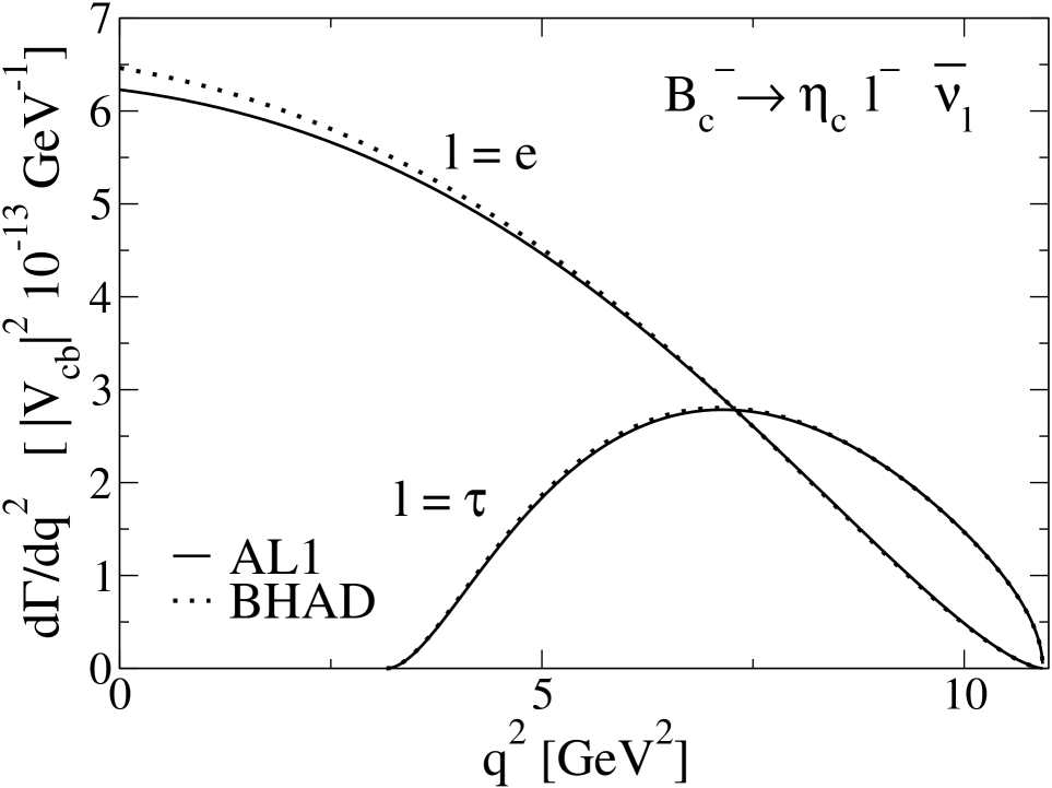
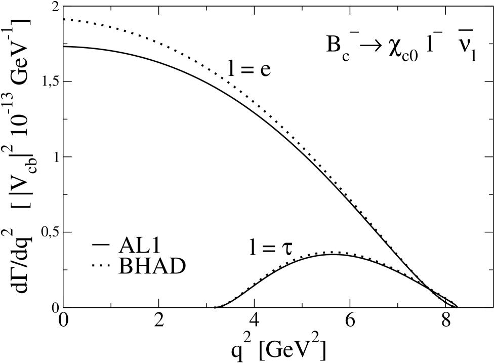
Figure 4.5: Differential decay width for the $B_{c}^{-}\to\eta_{c}l^{-}\bar{\nu}_{l}$ and $B_{c}^{-}\to\chi_{c0}l^{-}\bar{\nu}_{l}$ processes obtained with the AL1 potential. For comparison, we also show with dotted lines the results obtained with the Bhaduri (BHAD) potential. The distribution for a final muon is not explicitly shown. It differs appreciably from the corresponding to a final electron only for $q^{2}$ around $m_{\mu}^{2}$.

In Table 4.6 we give our results for the partial helicity widths corresponding to $B_{c}^{-}$ decays. For $B_{c}^{+}$ decay the “$P$” column changes sign while all others remain the same. The central values have been evaluated with the AL1 potential and the theoretical errors quoted reflect the dependence of the results on the inter-quark potential.

In Table 4.7 we show the asymmetry parameters. Our values for $\alpha^{*}$ compare well with the results obtained in Ref. [163]. The same is true for the forward–backward asymmetry with some exceptions: most notably we get opposite signs for $B_{c}\to\chi_{c1}$ and $B_{c}\to\Psi(3836)$.

In Fig. 4.5 we show the differential decay width $d\Gamma/dq^{2}$ for the decay channels $\eta_{c}l^{-}\bar{\nu}_{l}$ and $\chi_{c0}l^{-}\bar{\nu}_{l}$ for the case where the final lepton is a light one $l=e,\mu$ or a heavy one $l=\tau$. We show the results obtained with the AL1 and BHAD potentials, finding no significant difference for the $\tau$ case, while for the light final lepton case the differences are around 10% at low $q^{2}$.

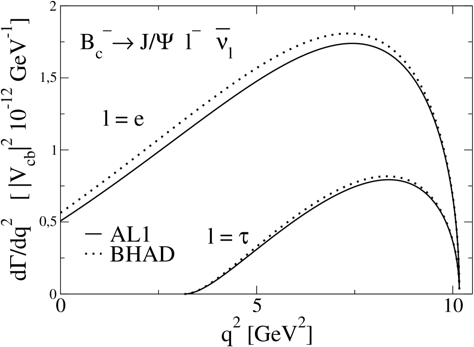
Figure 4.6: Differential decay width for the $B_{c}^{-}\to J/\Psi l^{-}\bar{\nu}_{l}$, $B_{c}^{-}\to h_{c}l^{-}\bar{\nu}_{l}$, $B_{c}^{-}\to\chi_{c1}l^{-}\bar{\nu}_{l}$, $B_{c}^{-}\to\chi_{c2}l^{-}\bar{\nu}_{l}$ and $B_{c}^{-}\to\Psi(3836)l^{-}\bar{\nu}_{l}$ decay channels obtained with the AL1 potential (solid lines) and the Bhaduri (BHAD) potential (dotted lines) . The distribution for a final muon is not explicitly shown. It differs appreciably from the corresponding to a final electron only for $q^{2}$ around $m_{\mu}^{2}$.

In Fig. 4.6 we show now the results for vector and tensor mesons. As before only for the case where the final lepton is light we see up to 10% differences between the calculation with the AL1 and the BHAD potentials.

Finally in Tables 4.8, 4.9 we give the total decay widths and corresponding branching ratios for the different transitions. The branching ratios evaluated by Ivanov et al. [162], where they have used the new $B_{c}$ mass determination by the CDF Collaboration [182], are in reasonable agreement with our results. Discrepancies are larger for the decay widths in Table 4.8 where they use the larger mass value $m_{B_{c}}=6400$ MeV quoted by the PDG [115].

	$\Gamma\ [10^{-15}\ \mathrm{GeV}]$
	This work	[163]	[165]	[167, 168]	[170]	[171]	[172]	[176]	[177]	[179]
$B^{-}_{c}\to\eta_{c}\,l^{-}\,\bar{\nu}_{l}$	$6.95^{+0.29}$	10.7	5.9	14.2	11.1	8.31	$11\pm 1$	2.1 (6.9)	8.6	10
$B^{-}_{c}\to\eta_{c}\,\tau^{-}\,\bar{\nu}_{\tau}$	$2.46^{+0.07}$	3.52							$3.3\pm 0.9$
$B^{-}_{c}\to\chi_{c0}\,l^{-}\,\bar{\nu}_{l}$	$1.55_{-0.02}^{+0.14}$	2.52		1.69
$B^{-}_{c}\to\chi_{c0}\,\tau^{-}\,\bar{\nu}_{\tau}$	$0.19^{+0.01}$	0.26		0.25
$B_{c}^{-}\to J/\Psi\,l^{-}\,\bar{\nu}_{l}$	$21.9^{+1.2}$	28.2	17.7	34.4	30.2	20.3	$28\pm 5$	21.6 (48.3)	17.2	42
$B_{c}^{-}\to J/\Psi\,\tau^{-}\,\bar{\nu}_{\tau}$	$5.86^{+0.23}_{-0.03}$	7.82							$7\pm 2$
$B_{c}^{-}\to\chi_{c1}\,l^{-}\,\bar{\nu}_{l}$	$0.94^{+0.05}_{-0.03}$	1.40		2.21
$B_{c}^{-}\to\chi_{c1}\,\tau^{-}\,\bar{\nu}_{\tau}$	$0.10$	0.17		0.35
$B_{c}^{-}\to h_{c}\,l^{-}\,\bar{\nu}_{l}$	$2.40^{+0.23}_{-0.01}$	4.42		2.51
$B_{c}^{-}\to h_{c}\,\tau^{-}\,\bar{\nu}_{\tau}$	$0.21^{+0.01}$	0.38		0.36
$B_{c}^{-}\to\chi_{c2}\,l^{-}\,\bar{\nu}_{l}$	$1.89^{+0.11}_{-0.08}$	2.92		2.73
$B_{c}^{-}\to\chi_{c2}\,\tau^{-}\,\bar{\nu}_{\tau}$	$0.13_{-0.01}^{+0.01}$	0.20		0.42
$B_{c}^{-}\to\Psi(3836)\,l^{-}\,\bar{\nu}_{l}$	$0.062_{-0.008}$	0.13
$B_{c}^{-}\to\Psi(3836)\,\tau^{-}\,\bar{\nu}_{\tau}$	$0.0012_{-0.0002}$	0.0031

Table 4.8: Decay widths in units of $10^{-15}$ GeV for semileptonic $B_{c}^{-}\to c\bar{c}$ decays. Our central values have been evaluated with the AL1 potential. Here $l$ stands for $l=e,\,\mu$.

hola

	B.R. (%)
	This work	[162]	[165]	[167, 168, 169]	[170]	[173, 174]	[176]	[177]	[178]
$B^{-}_{c}\to\eta_{c}\,l^{-}\,\bar{\nu}_{l}$	$0.48^{+0.02}$	0.81	0.42	0.97	0.76	0.75	0.15	0.59	0.51
$B^{-}_{c}\to\eta_{c}\,\tau^{-}\,\bar{\nu}_{\tau}$	$0.17^{+0.01}$	0.22				0.23		0.20
$B^{-}_{c}\to\chi_{c0}\,l^{-}\,\bar{\nu}_{l}$	$0.11^{+0.01}$	0.17		0.12
$B^{-}_{c}\to\chi_{c0}\,\tau^{-}\,\bar{\nu}_{\tau}$	$0.013^{+0.001}$	0.013		0.017
$B_{c}^{-}\to J/\Psi\,l^{-}\,\bar{\nu}_{l}$	$1.54^{+0.06}$	2.07	1.23	2.35	2.01	1.9	1.47	1.20	1.44
$B_{c}^{-}\to J/\Psi\,\tau^{-}\,\bar{\nu}_{\tau}$	$0.41^{+0.02}$	0.49				0.48		0.34
$B_{c}^{-}\to\chi_{c1}\,l^{-}\,\bar{\nu}_{l}$	$0.066^{+0.003}_{-0.002}$	0.092		0.15
$B_{c}^{-}\to\chi_{c1}\,\tau^{-}\,\bar{\nu}_{\tau}$	$0.0072^{+0.0002}_{-0.0003}$	0.0089		0.024
$B_{c}^{-}\to h_{c}\,l^{-}\,\bar{\nu}_{l}$	$0.17^{+0.02}$	0.27		0.17
$B_{c}^{-}\to h_{c}\,\tau^{-}\,\bar{\nu}_{\tau}$	$0.015^{+0.001}$	0.017		0.024
$B_{c}^{-}\to\chi_{c2}\,l^{-}\,\bar{\nu}_{l}$	$0.13^{+0.01}$	0.17		0.19
$B_{c}^{-}\to\chi_{c2}\,\tau^{-}\,\bar{\nu}_{\tau}$	$0.0093^{+0.0002}_{-0.0005}$	0.0082		0.029
$B_{c}^{-}\to\Psi(3836)\,l^{-}\,\bar{\nu}_{l}$	$0.0043_{-0.0005}$	0.0066
$B_{c}^{-}\to\Psi(3836)\,\tau^{-}\,\bar{\nu}_{\tau}$	$0.000083_{-0.000010}$	0.000099

Table 4.9: Branching ratios in % for semileptonic $B_{c}^{-}\to c\bar{c}$ decays. Our central values have been evaluated with the AL1 potential. Here $l$ stands for $l=e,\,\mu$.

4.3.3 Heavy quark spin symmetry

As mentioned in the introduction one can not apply HQS to systems with two heavy quarks due to flavor symmetry breaking by the kinetic energy terms. The symmetry that survives for such systems is HQSS amounting to the decoupling of the two heavy quark spins. Using HQSS Jenkins et al. [72] obtained relations between different form factors for semileptonic $B_{c}$ decays into ground state vector and pseudoscalar mesons. Let us check the agreement of our calculations with their results. For that purpose let us re-write the general form factor decompositions in Eq. (4.3.1) introducing the four vectors $v$ and $k$ such that

$$P_{B_{c}}=m_{B_{c}}\,v\hskip 14.22636pt;\hskip 14.22636ptP_{c\bar{c}}=m_{c\bar{c}}\,v+k$$ (4.45)

$v$ is the four-velocity of the initial $B_{c}$ meson whereas $k$ is a residual momentum. In terms of those we have

$$P=P_{B_{c}}+P_{c\bar{c}}=(m_{B_{c}}+m_{c\bar{c}})\,v+k$$ (4.46)

$$q=P_{B_{c}}-P_{c\bar{c}}=(m_{B_{c}}-m_{c\bar{c}})\,v-k$$ (4.47)

and we can write for the $\eta_{c}\,(c\bar{c}\,(0^{-}))$ final state case

$$\left\langle\,\eta_{c},\,\vec{P}_{\eta_{c}}\,\left|\,J^{c\,b}_{\mu}(0)\,\right|\,B_{c}^{-},\,\vec{P}_{B_{c}}\right\rangle = \left\langle\,\eta_{c},\,\vec{P}_{\eta_{c}}\,\left|\hskip 8.5359ptJ^{c\,b}_{V\,\mu}(0)\,\right|\,B_{c}^{-},\,\vec{P}_{B_{c}}\right\rangle$$ (4.48)

$$= \left((m_{B_{c}}+m_{\eta_{c}})\,F_{+}(q^{2})+(m_{B_{c}}-m_{\eta_{c}})\,F_{-}(q^{2})\right)\,v_{\mu}$$

$$\hskip 14.22636pt+(F_{+}(q^{2})-F_{-}(q^{2}))\,k_{\mu}$$

$$= \sqrt{2m_{B_{c}}2m_{\eta_{c}}}\left(\Sigma_{1}^{(0^{-})}(q^{2})\,v_{\mu}+\overline{\Sigma}_{2}^{(0^{-})}(q^{2})\,k_{\mu}\right)$$

where we have introduced the new form factors

$$\Sigma_{1}^{(0^{-})}(q^{2}) = \frac{1}{\sqrt{2m_{B_{c}}2m_{\eta_{c}}}}\,\left((m_{B_{c}}+m_{\eta_{c}})\,F_{+}(q^{2})+(m_{B_{c}}-m_{\eta_{c}})\,F_{-}(q^{2})\right)$$

$$\overline{\Sigma}_{2}^{(0^{-})}(q^{2}) = \frac{1}{\sqrt{2m_{B_{c}}2m_{\eta_{c}}}}\,(F_{+}(q^{2})-F_{-}(q^{2}))$$ (4.49)

Similarly for the $J/\Psi\,(c\bar{c}\,(1^{-}))$ final state case we have

$$\left\langle\,J/\Psi,\,\lambda\,\vec{P}_{J/\Psi}\,\left|\,J^{c\,b}_{\mu}(0)\,\right|\,B_{c}^{-},\,\vec{P}_{B_{c}}\right\rangle\,=$$ (4.50)

$$= \left\langle\,J/\Psi,\,\lambda\,\vec{P}_{J/\Psi}\,\left|\,J^{c\,b}_{V\mu}(0)-J^{c\,b}_{A\mu}(0)\,\right|\,B_{c}^{-},\,\vec{P}_{B_{c}}\right\rangle$$

$$= \frac{2m_{B_{c}}}{m_{B_{c}}+m_{J/\Psi}}\varepsilon_{\mu\nu\alpha\beta}\ \varepsilon^{\,\nu\,*}_{(\lambda)}(\,\vec{P}_{J/\Psi}\,)\,v^{\alpha}\,k^{\,\beta}\,V(q^{2})$$

$$-\,i\,\bigg{\{}\ (m_{B_{c}}-m_{J/\Psi})\ \varepsilon_{(\lambda)\,\mu}^{*}(\,\vec{P}_{J/\Psi}\,)\,A_{0}(q^{2})$$

$$\hskip 22.76228pt+\frac{m_{B_{c}}}{m_{J/\Psi}}{k\cdot\varepsilon^{*}_{(\lambda)}(\,\vec{P}_{J/\Psi}\,)}\bigg{(}\ \frac{A_{+}(q^{2})}{m_{B_{c}}+m_{J/\Psi}}\left((m_{B_{c}}+m_{J/\Psi})\,v_{\mu}+k_{\mu}\right)$$

$$\hskip 113.81102pt+\frac{A_{-}(q^{2})}{m_{B_{c}}+m_{J/\Psi}}\left((m_{B_{c}}-m_{J/\Psi})\,v_{\mu}-k_{\mu}\right)\bigg{)}\bigg{\}}$$

$$= -\sqrt{2m_{B_{c}}2m_{J/\Psi}}\,\varepsilon_{\mu\nu\alpha\beta}\ \varepsilon^{\,\nu\,*}_{(\lambda)}(\,\vec{P}_{J/\Psi}\,)\,v^{\alpha}\,k^{\,\beta}\,\overline{\Sigma}^{\prime(1^{-})}_{2}(q^{2})$$

$$-i\sqrt{2m_{B_{c}}2m_{J/\Psi}}\bigg{\{}\ \varepsilon^{*}_{(\lambda)\,\mu}(\,\vec{P}_{J/\Psi}\,)\,\Sigma_{1}^{(1^{-})}(q^{2})$$

$$\hskip 72.55461pt+\left(k\cdot\varepsilon^{*}_{(\lambda)}(\,\vec{P}_{J/\Psi}\,)\right)\,\overline{\Sigma}_{2}^{(1^{-})}(q^{2})\,v_{\mu}$$

$$\hskip 72.55461pt+\left(k\cdot\varepsilon^{*}_{(\lambda)}(\,\vec{P}_{J/\Psi}\,)\right)\,\overline{\Sigma}_{3}^{(1^{-})}(q^{2})\,k_{\mu}\bigg{\}}$$

with

$$\Sigma_{1}^{(1^{-})}(q^{2}) = \frac{1}{\sqrt{2m_{B_{c}}2m_{J/\Psi}}}\,\left(m_{B_{c}}-m_{J/\Psi}\right)\,A_{0}(q^{2})$$

$$\overline{\Sigma}_{2}^{(1^{-})}(q^{2}) = \frac{1}{\sqrt{2m_{B_{c}}2m_{J/\Psi}}}\,\frac{m_{B_{c}}}{m_{J/\Psi}}\,\left(\,A_{+}(q^{2})+\frac{m_{B_{c}}-m_{J/\Psi}}{m_{B_{c}}+m_{J/\Psi}}\,A_{-}(q^{2})\right)$$

$$\overline{\Sigma}_{2}^{\prime(1^{-})}(q^{2}) = \frac{1}{\sqrt{2m_{B_{c}}2m_{J/\Psi}}}\,\frac{-2m_{B_{c}}}{m_{B_{c}}+m_{J/\Psi}}\,V(q^{2})$$

$$\overline{\Sigma}_{3}^{(1^{-})}(q^{2}) = \frac{1}{\sqrt{2m_{B_{c}}2m_{J/\Psi}}}\,\frac{m_{B_{c}}}{m_{J/\Psi}}\,\frac{1}{m_{B_{c}}+m_{J/\Psi}}\left(A_{+}(q^{2})-A_{-}(q^{2})\right)$$ (4.51)

$\Sigma_{1}^{(0^{-})}$ and $\Sigma_{1}^{(1^{-})}$ are dimensionless, $\overline{\Sigma}_{2}^{(0^{-})}$, $\overline{\Sigma}_{2}^{(1^{-})}$, $\overline{\Sigma}_{2}^{\prime(1^{-})}$ have dimensions of $E^{-1}$, and $\overline{\Sigma}_{3}^{(1^{-})}$ has dimensions of $E^{-2}$.

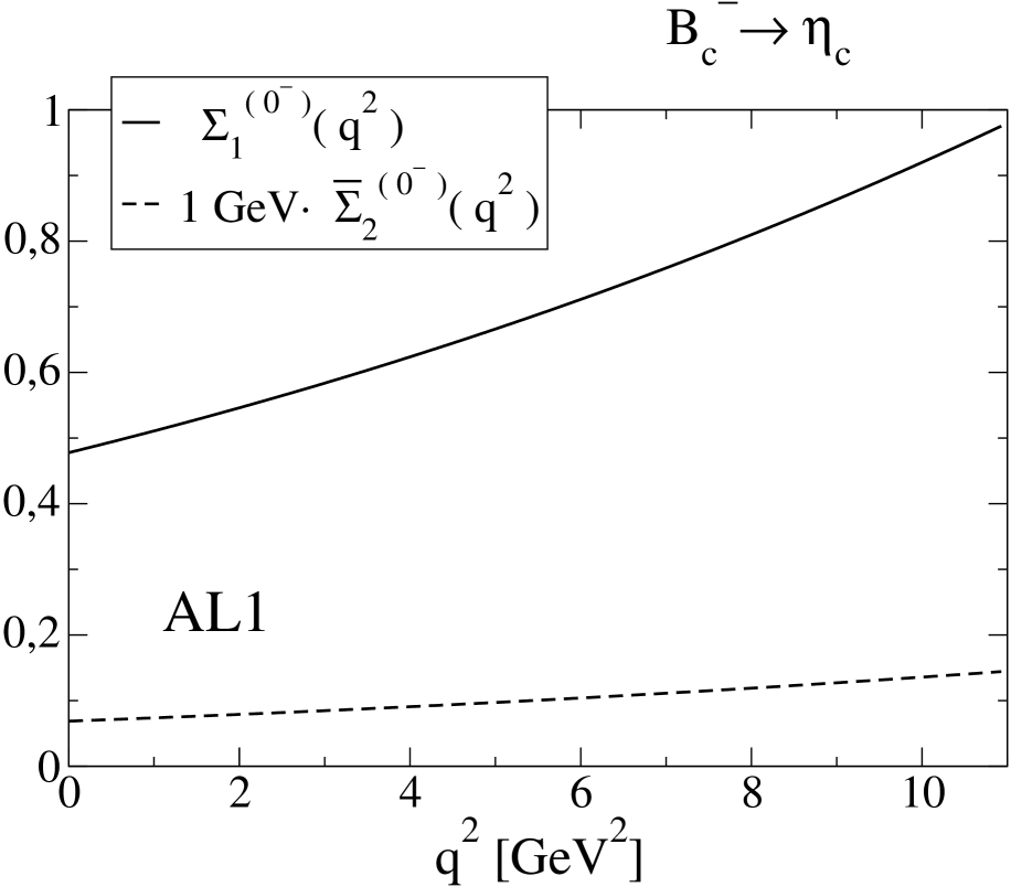
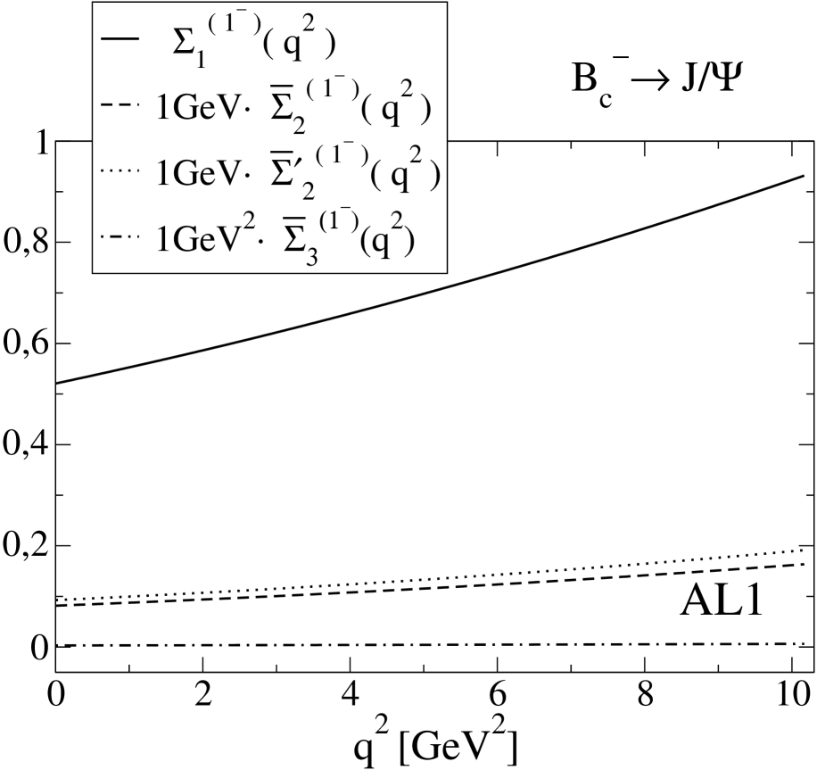
Figure 4.7: $\Sigma_{1}^{(0^{-})}$ (solid line) and $\overline{\Sigma}_{2}^{(0^{-})}$ (dashed line) of the $B_{c}^{-}\to\eta_{c}$, and ${\Sigma}_{1}^{(1^{-})}$ (solid line), $\overline{\Sigma}_{2}^{(1^{-})}$ (dashed line), $\overline{\Sigma}^{\prime\,(1^{-})}_{2}$ (dotted line) and $\overline{\Sigma}_{3}^{(1^{-})}$ (dashed–dotted line) of the $B_{c}^{-}\to J/\Psi$ semileptonic decays evaluated with the AL1 potential.

We can take the infinite heavy quark mass limit $m_{b}\gg m_{c}\gg\Lambda_{QCD}$ with the result that near zero recoil

$$\Sigma_{1}^{(0^{-})}=\Sigma_{1}^{(1^{-})}$$

$$\overline{\Sigma}_{2}^{(0^{-})}=\overline{\Sigma}_{2}^{(1^{-})}=\overline{\Sigma}_{2}^{\prime(1^{-})}=0$$

$$\overline{\Sigma}_{3}^{(1^{-})}=0$$ (4.52)

This agrees perfectly with the result obtained in Ref. [72] using HQSS.

In Fig. 4.7 we give our results for the above quantities for the semileptonic $B_{c}^{-}\to\eta_{c}$ and $B_{c}^{-}\to J/\Psi$ decays for the actual heavy quark masses. Even though we are not in the infinite heavy quark mass limit we find that $\Sigma_{1}^{(0^{-})}$ and $\Sigma_{1}^{(1^{-})}$ dominate over the whole $q^{2}$ interval. This dominant behavior would be more so near the zero–recoil point where $k\approx 0$ and thus the contributions from the terms in $\overline{\Sigma}_{2}^{(0^{-})}$, $\overline{\Sigma}_{2}^{(1^{-})}$, $\overline{\Sigma}_{2}^{\prime(1^{-})}$ and $\overline{\Sigma}_{3}^{(1^{-})}$ are even more suppressed. Thus, even for the actual heavy quark masses we find that near zero recoil

$$\left\langle\,\eta_{c},\,\vec{P}_{\eta_{c}}\,\left|\,J^{c\,b}_{\mu}(0)\,\right|\,B_{c}^{-},\,\vec{P}_{B_{c}}\right\rangle \approx \sqrt{2m_{B_{c}}2m_{\eta_{c}}}\ \Sigma_{1}^{(0^{-})}(q^{2})\,v_{\mu}$$

$$\left\langle\,J/\Psi,\,\lambda\,\vec{P}_{J/\Psi}\,\left|\,J^{c\,b}_{\mu}(0)\,\right|\,B_{c}^{-},\,\vec{P}_{B_{c}}\right\rangle \approx -i\sqrt{2m_{B_{c}}2m_{J/\Psi}}\ \varepsilon^{*}_{(\lambda)\,\mu}(\,\vec{P}_{J/\Psi}\,)\,\Sigma_{1}^{(1^{-})}(q^{2})$$

Besides, as seen in In Fig. 4.8, $\Sigma_{1}^{(0^{-})}$ of the $B_{c}^{-}\to\eta_{c}$, and ${\Sigma}_{1}^{(1^{-})}$ of the $B_{c}^{-}\to J/\Psi$ semileptonic decays are very close to each other over the whole $q^{2}$ interval. This implies that the result obtained in Ref. [72] near zero recoil using HQSS seems to be valid, to a very good approximation, outside the infinite heavy quark mass limit.

Figure 4.8: $\Sigma_{1}^{(0^{-})}$ (solid line) of the $B_{c}^{-}\to\eta_{c}$, and ${\Sigma}_{1}^{(1^{-})}$ (dashed line) of the $B_{c}^{-}\to J/\Psi$ semileptonic decays evaluated with the AL1 potential.

4.4 Nonleptonic $B_{c}^{-}\to c\bar{c}\ M_{F}^{-}$ two–meson decays.

In this section we will evaluate decay widths for nonleptonic $B_{c}^{-}\to c\bar{c}\ M_{F}^{-}$ two–meson decays where $M_{F}^{-}$ is a pseudoscalar or vector meson. These decay modes involve a $b\to c$ transition at the quark level and they are governed, neglecting penguin operators, by the effective Hamiltonian  [165, 176, 162]

$$H_{eff.}=\frac{G_{F}}{\sqrt{2}}\,\left\{V_{cb}\left[c_{1}(\mu)\,Q_{1}^{cb}+c_{2}(\mu)\,Q_{2}^{cb}\right]+H.c.\right\}$$ (4.54)

where $c_{1},\,c_{2}$ are scale–dependent Wilson coefficients, and $Q_{1}^{cb},\,Q_{2}^{cb}$ are local four–quark operators given by

$$Q_{1}^{cb} = \overline{\Psi}_{c}(0)\gamma_{\mu}(I-\gamma_{5})\Psi_{b}(0)\,\bigg{[}\ V_{ud}^{*}\,\overline{\Psi}_{d}(0)\gamma^{\mu}(I-\gamma_{5})\Psi_{u}(0)+V_{us}^{*}\,\overline{\Psi}_{s}(0)\gamma^{\mu}(I-\gamma_{5})\Psi_{u}(0)$$

$$\hskip 99.58464pt+V_{cd}^{*}\,\overline{\Psi}_{d}(0)\gamma^{\mu}(I-\gamma_{5})\Psi_{c}(0)+V_{cs}^{*}\,\overline{\Psi}_{s}(0)\gamma^{\mu}(I-\gamma_{5})\Psi_{c}(0)\,\bigg{]}$$

$$Q_{2}^{cb} = \overline{\Psi}_{d}(0)\gamma_{\mu}(I-\gamma_{5})\Psi_{b}(0)\,\bigg{[}\ V_{ud}^{*}\,\overline{\Psi}_{c}(0)\gamma^{\mu}(I-\gamma_{5})\Psi_{u}(0)+V_{cd}^{*}\,\overline{\Psi}_{c}(0)\gamma^{\mu}(I-\gamma_{5})\Psi_{c}(0)\,\bigg{]}$$

$$+\overline{\Psi}_{s}(0)\gamma_{\mu}(I-\gamma_{5})\Psi_{b}(0)\,\bigg{[}V_{us}^{*}\,\overline{\Psi}_{c}(0)\gamma^{\mu}(I-\gamma_{5})\Psi_{u}(0)\,+V_{cs}^{*}\,\overline{\Psi}_{c}(0)\gamma^{\mu}(I-\gamma_{5})\Psi_{c}(0)\bigg{]}$$

where the different $V_{jk}$ are CKM matrix elements.

We shall work in the factorization approximation which amounts to evaluate the hadron matrix elements of the effective Hamiltonian as a product of quark–current matrix elements: one of these is the matrix element for the $B_{c}^{-}$ transition to one of the final mesons, while the other matrix element corresponds to the transition from the vacuum to the other final meson. The latter is given by the corresponding meson decay constant. This factorization approximation is schematically represented in Fig. 4.9.

Figure 4.9: Diagrammatic representation of $B_{c}^{-}$ two–meson decay in the factorization approximation.

When writing the factorization amplitude one has to take into account the Fierz reordered contribution so that the relevant coefficients are not $c_{1}$ and $c_{2}$ but the combinations

$$a_{1}(\mu)=c_{1}(\mu)+\frac{1}{N_{C}}\,c_{2}(\mu)\hskip 14.22636pt;\hskip 14.22636pta_{2}(\mu)=c_{2}(\mu)+\frac{1}{N_{C}}\,c_{1}(\mu)$$ (4.56)

with $N_{C}=3$ the number of colors. The energy scale $\mu$ appropriate in this case is $\mu\simeq m_{b}$ and the values for $a_{1}$ and $a_{2}$ that we use are [162]

$$a_{1}=1.14\hskip 14.22636pt;\hskip 14.22636pta_{2}=-0.20$$ (4.57)

$\bullet$ $M_{F}^{-}=\pi^{-},\,\rho^{-},\,K^{-},\,K^{*-}$

	$\Gamma\ [10^{-15}\ \mathrm{GeV}]$
$B_{c}^{-}\to\eta_{c}\,\pi^{-}$	$1.02^{+0.07}\,a_{1}^{2}$
$B_{c}^{-}\to\eta_{c}\,\rho^{-}$	$2.60^{+0.16}\,a_{1}^{2}$
$B_{c}^{-}\to\eta_{c}\,K^{-}$	$0.082^{+0.004}\,a_{1}^{2}$
$B_{c}^{-}\to\eta_{c}\,K^{*-}$	$0.15^{+0.01}\,a_{1}^{2}$
$B_{c}^{-}\to J/\Psi\,\pi^{-}$	$0.83^{+0.09}\,a_{1}^{2}$
$B_{c}^{-}\to J/\Psi\,\rho^{-}$	$2.61^{+0.27}\,a_{1}^{2}$
$B_{c}^{-}\to J/\Psi\,K^{-}$	$0.065^{+0.007}\,a_{1}^{2}$
$B_{c}^{-}\to J/\Psi\,K^{*-}$	$0.16^{+0.01}\,a_{1}^{2}$
$B_{c}^{-}\to\chi_{c0}\,\pi^{-}$	$0.28^{+0.03}\,a_{1}^{2}$
$B_{c}^{-}\to\chi_{c0}\,\rho^{-}$	$0.73^{+0.07}\,a_{1}^{2}$
$B_{c}^{-}\to\chi_{c0}\,K^{-}$	$0.022^{+0.003}\,a_{1}^{2}$
$B_{c}^{-}\to\chi_{c0}\,K^{*-}$	$0.041^{+0.005}\,a_{1}^{2}$
$B_{c}^{-}\to\chi_{c1}\,\pi^{-}$	$0.0015^{+0.0002}\,a_{1}^{2}$
$B_{c}^{-}\to\chi_{c1}\,\rho^{-}$	$0.11^{+0.01}\,a_{1}^{2}$
$B_{c}^{-}\to\chi_{c1}\,K^{-}$	$0.00012^{+0.00001}\,a_{1}^{2}$
$B_{c}^{-}\to\chi_{c1}\,K^{*-}$	$0.0080^{+0.0007}_{-0.0002}\,a_{1}^{2}$
$B_{c}^{-}\to h_{c}\,\pi^{-}$	$0.58^{+0.07}\,a_{1}^{2}$
$B_{c}^{-}\to h_{c}\,\rho^{-}$	$1.41^{+0.17}\,a_{1}^{2}$
$B_{c}^{-}\to h_{c}\,K^{-}$	$0.045^{+0.006}\,a_{1}^{2}$
$B_{c}^{-}\to h_{c}\,K^{*-}$	$0.078^{+0.009}\,a_{1}^{2}$
$B_{c}^{-}\to\chi_{c2}\,\pi^{-}$	$0.24^{+0.02}\,a_{1}^{2}$
$B_{c}^{-}\to\chi_{c2}\,\rho^{-}$	$0.71^{+0.07}_{-0.03}\,a_{1}^{2}$
$B_{c}^{-}\to\chi_{c2}\,K^{-}$	$0.018^{+0.002}\,a_{1}^{2}$
$B_{c}^{-}\to\chi_{c2}\,K^{*-}$	$0.041^{+0.004}_{-0.001}\,a_{1}^{2}$
$B_{c}^{-}\to\Psi(3836)\,\pi^{-}$	$0.00045^{+0.00003}_{-0.00003}\,a_{1}^{2}$
$B_{c}^{-}\to\Psi(3836)\,\rho^{-}$	$0.021^{+0.001}_{-0.002}\,a_{1}^{2}$
$B_{c}^{-}\to\Psi(3836)\,K^{-}$	$0.000034^{+0.000002}_{-0.000002}\,a_{1}^{2}$
$B_{c}^{-}\to\Psi(3836)\,K^{*-}$	$0.0015_{-0.0002}\,a_{1}^{2}$

Table 4.10: Decay widths in units of $10^{-15}$ GeV, and for general values of the Wilson coefficient $a_{1}$, for exclusive nonleptonic decays of the $B_{c}^{-}$ meson. Our central values have been obtained with the AL1 potential.

This is the simplest case. The decay width is given by

$$\Gamma=\frac{G_{F}^{2}}{16\pi m^{2}_{B_{c}}}\,|V_{cb}|^{2}\,|V_{F}|^{2}\ a_{1}^{2}\,\frac{\lambda^{1/2}(m^{2}_{B_{c}},\,m^{2}_{c\bar{c}},\,m^{2}_{F})}{2m_{B_{c}}}\,{\cal H}_{\alpha\beta}(P_{B_{c}},P_{c\bar{c}})\,\widehat{\cal H}^{{\alpha\beta}}(P_{F})$$

with $m_{F}$ the mass of the $M_{F}^{-}$ final meson, and $V_{F}=V_{ud}$ or $V_{F}=V_{us}$ depending on whether $M_{F}^{-}=\pi^{-},\,\rho^{-}$ or $M_{F}^{-}=K^{-},\,K^{*-}$. ${\cal H}_{\alpha\beta}(P_{B_{c}},P_{c\bar{c}})$ is the hadron tensor for the $B_{c}^{-}\to c\bar{c}$ transition and $\widehat{\cal H}^{{\alpha\beta}}(P_{F})$ is the hadron tensor for the $\mathrm{vacuum}\to M_{F}^{-}$ transition. The latter is

$$\widehat{\cal H}^{{\alpha\beta}}(P_{F}) = P_{F}^{\alpha}\,P_{F}^{\beta}\,f_{F}^{2}\hskip 119.50148ptM_{F}^{-}\equiv 0^{-}\ \mathrm{case}$$

$$\widehat{\cal H}^{{\alpha\beta}}(P_{F}) = (P_{F}^{\alpha}\,P_{F}^{\beta}\,-m_{F}^{2}\,g^{\alpha\,\beta})f_{F}^{2}\hskip 61.17325ptM_{F}^{-}\equiv 1^{-}\ \mathrm{case}$$ (4.59)

with $f_{F}$ being the $M_{F}^{-}$ decay constant.

Similarly to the semileptonic case, the product ${\cal H}_{\alpha\beta}(P_{B_{c}},P_{c\bar{c}})\ \widehat{\cal H}^{{\alpha\beta}}(P_{F})$ can now be easily written in terms of helicity amplitudes for the $B_{c}^{-}\to c\bar{c}$ transition so that the width is given as [162]

$$M_{F}^{-}\equiv 0^{-}\ \mathrm{case}$$

$$\Gamma=\frac{G_{F}^{2}}{16\pi m^{2}_{B_{c}}}\,|V_{cb}|^{2}\,|V_{F}|^{2}\ a_{1}^{2}\,\frac{\lambda^{1/2}(m^{2}_{B_{c}},\,m^{2}_{c\bar{c}},\,m^{2}_{F})}{2m_{B_{c}}}\,m_{F}^{2}\,f^{2}_{F}\,{\cal H}^{B_{c}^{-}\to c\bar{c}}_{tt}(m_{F}^{2})$$

$$M_{F}^{-}\equiv 1^{-}\ \mathrm{case}$$

$$\Gamma=\frac{G_{F}^{2}}{16\pi m^{2}_{B_{c}}}\,|V_{cb}|^{2}\,|V_{F}|^{2}\ a_{1}^{2}\ \frac{\lambda^{1/2}(m^{2}_{B_{c}},\,m^{2}_{c\bar{c}},\,m^{2}_{F})}{2m_{B_{c}}}\,m_{F}^{2}\,f^{2}_{F}$$

$$\hskip 56.9055pt\times\left({\cal H}^{B_{c}^{-}\to c\bar{c}}_{+1+1}(m_{F}^{2})+{\cal H}^{B_{c}^{-}\to c\bar{c}}_{-1-1}(m_{F}^{2})+{\cal H}_{00}^{B_{c}^{-}\to c\bar{c}}(m_{F}^{2})\right)$$ (4.60)

with the different ${\cal H}_{rr}$ evaluated at $q^{2}=m_{F}^{2}$. In Table 4.10 we show the decay widths for a general value of the Wilson coefficient $a_{1}$, whereas in Table 4.11 we give the corresponding branching ratios evaluated with $a_{1}=1.14$. Our results for a final $\eta_{c}$ or $J/\psi$ are in good agreement with the ones obtained by Ebert et al. [165], El-Hady et al. [170] and Anisimov et al. [177], but they are a factor 2 smaller than the results by Ivanov et al. [162] and Kiselev [174]. Large discrepancies with Ivanov’s results show up for the other transitions.

	B.R. (%)
	This work	[162]	[165]	[167, 168, 169]	[170]	[174, 175]	[176]	[177]	[180]
$B_{c}^{-}\to\eta_{c}\,\pi^{-}$	$0.094^{+0.006}$	0.19	0.083	0.18	0.14	0.20	0.025	0.13
$B_{c}^{-}\to\eta_{c}\,\rho^{-}$	$0.24^{+0.01}$	0.45	0.20	0.49	0.33	0.42	0.067	0.30
$B_{c}^{-}\to\eta_{c}\,K^{-}$	$0.0075^{+0.0005}$	0.015	0.006	0.014	0.011	0.013	0.002	0.013
$B_{c}^{-}\to\eta_{c}\,K^{*-}$	$0.013^{+0.001}$	0.025	0.011	0.025	0.018	0.020	0.004	0.021
$B_{c}^{-}\to J/\Psi\,\pi^{-}$	$0.076^{+0.008}$	0.17	0.060	0.18	0.11	0.13	0.13	0.073
$B_{c}^{-}\to J/\Psi\,\rho^{-}$	$0.24^{+0.02}$	0.49	0.16	0.53	0.31	0.40	0.37	0.21
$B_{c}^{-}\to J/\Psi\,K^{-}$	$0.0060^{+0.0006}$	0.013	0.005	0.014	0.008	0.011	0.007	0.007
$B_{c}^{-}\to J/\Psi\,K^{*-}$	$0.014^{+0.002}$	0.028	0.010	0.029	0.018	0.022	0.020	0.016
$B_{c}^{-}\to\chi_{c0}\,\pi^{-}$	$0.026^{+0.003}$	0.055		0.028		0.98
$B_{c}^{-}\to\chi_{c0}\,\rho^{-}$	$0.067^{+0.006}_{-0.001}$	0.13		0.072		3.29
$B_{c}^{-}\to\chi_{c0}\,K^{-}$	$0.0020^{+0.0002}$	0.0042		0.00021
$B_{c}^{-}\to\chi_{c0}\,K^{*-}$	$0.0037^{+0.0005}$	0.0070		0.00039
$B_{c}^{-}\to\chi_{c1}\,\pi^{-}$	$0.00014^{+0.00001}$	0.0068		0.007		0.0089
$B_{c}^{-}\to\chi_{c1}\,\rho^{-}$	$0.010^{+0.001}_{-0.001}$	0.029		0.029		0.46
$B_{c}^{-}\to\chi_{c1}\,K^{-}$	$1.1^{+0.1}\,10^{-5}$	5.1 $10^{-4}$		5.2 $10^{-5}$
$B_{c}^{-}\to\chi_{c1}\,K^{*-}$	$0.00073^{+0.00007}_{-0.00002}$	0.0018		0.00018
$B_{c}^{-}\to h_{c}\,\pi^{-}$	$0.053^{+0.007}$	0.11		0.05		1.60
$B_{c}^{-}\to h_{c}\,\rho^{-}$	$0.13^{+0.01}$	0.25		0.12		5.33
$B_{c}^{-}\to h_{c}\,K^{-}$	$0.0041^{+0.0006}$	0.0083		0.00038
$B_{c}^{-}\to h_{c}\,K^{*-}$	$0.0071^{+0.0008}$	0.013		0.00068
$B_{c}^{-}\to\chi_{c2}\,\pi^{-}$	$0.022^{+0.002}$	0.046		0.025		0.79			0.0076
$B_{c}^{-}\to\chi_{c2}\,\rho^{-}$	$0.065^{+0.006}_{-0.002}$	0.12		0.051		3.20			0.023
$B_{c}^{-}\to\chi_{c2}\,K^{-}$	$0.0017^{+0.0001}$	0.0034		0.00018					0.00056
$B_{c}^{-}\to\chi_{c2}\,K^{*-}$	$0.0038^{+0.0003}_{-0.0002}$	0.0065		0.00031					0.0013
$B_{c}^{-}\to\Psi(3836)\,\pi^{-}$	$4.1^{+0.03}_{-0.02}\,10^{-5}$	0.0017				0.030
$B_{c}^{-}\to\Psi(3836)\,\rho^{-}$	$0.0020_{-0.0003}$	0.0055				0.98
$B_{c}^{-}\to\Psi(3836)\,K^{-}$	$3.1^{+0.2}_{-0.2}\,10^{-6}$	0.00012
$B_{c}^{-}\to\Psi(3836)\,K^{*-}$	$0.00014_{-0.00002}$	0.00032

Table 4.11: Branching ratios in % for exclusive nonleptonic decays of the $B_{c}^{-}$ meson. Our central values have been obtained with the AL1 potential.

$\bullet$ $M_{F}^{-}=D^{-},\,D^{*-},\,D_{s}^{-},\,D_{s}^{*-}$

In this subsection we shall evaluate the nonleptonic two–meson $B_{c}^{-}\to\eta_{c}D^{-},$ $\eta_{c}D^{*-},\,J/\Psi D^{-},\,J/\Psi\,D^{*-}$ and $B_{c}^{-}\to\eta_{c}D_{s}^{-},\,\eta_{c}D_{s}^{*-},\,J/\Psi D_{s}^{-},\,J/\Psi\,D_{s}^{*-}$ decay widths. In these cases there are two different contributions in the factorization approximation. Following the same steps that lead to Eq.(4.60) we shall get

$$\Gamma=\frac{G_{F}^{2}}{16\pi m^{2}_{B_{c}}}\,|V_{cb}|^{2}\,|V_{F}|^{2}\,\frac{\lambda^{1/2}(m^{2}_{B_{c}},\,m^{2}_{c\bar{c}},\,m^{2}_{F})}{2m_{B_{c}}}\ {\cal HH}$$ (4.61)

where now $V_{F}=V_{cd}$ for $M_{F}^{-}=D^{-},D^{*-}$ and $V_{F}=V_{cs}$ for $M_{F}^{-}=D_{s}^{-},D_{s}^{*-}$. The quantity ${\cal HH}$ incorporates all information on the hadron matrix elements and depends on the transition as [162]

$${\cal HH}^{B_{c}^{-}\to\eta_{c}D^{-}} = \left|a_{1}\,h_{t}^{B_{c}^{-}\to\eta_{c}}(m^{2}_{D^{-}})\,m_{D^{-}}\,f_{D^{-}}+a_{2}\,h_{t}^{B_{c}^{-}\to D^{-}}(m_{\eta_{c}}^{2})\,m_{\eta_{c}}\,f_{\eta_{c}}\right|^{2}$$

$${\cal HH}^{B_{c}^{-}\to\eta_{c}D^{*-}} = \left|-a_{1}\,h_{0}^{B_{c}^{-}\to\eta_{c}}(m^{2}_{D^{*-}})\,m_{D^{*-}}\,f_{D^{*-}}+a_{2}\,i\,h_{(0)\,t}^{B_{c}^{-}\to D^{*-}}(m_{\eta_{c}}^{2})\,m_{\eta_{c}}\,f_{\eta_{c}}\right|^{2}$$

$${\cal HH}^{B_{c}^{-}\to J/\Psi D^{-}} = \left|a_{1}\,i\,h_{(0)\,t}^{B_{c}^{-}\to J/\Psi}(m_{D^{-}}^{2})\,m_{D^{-}}\,f_{D^{-}}-a_{2}\,\,h_{0}^{B_{c}^{-}\to D^{-}}(m_{J/\Psi}^{2})\,m_{J/\Psi}\,f_{J/\Psi}\right|^{2}$$

$${\cal HH}^{B_{c}^{-}\to J/\Psi D^{*-}} = \sum_{r=+1,\,-1,\,0}\,\left|a_{1}\,\,h_{(r)\,r}^{B_{c}^{-}\to J/\Psi}(m_{D^{*-}}^{2})\,m_{D^{*-}}\,f_{D^{*-}}\right.$$ (4.62)

$$\hskip 56.9055pt\left.+a_{2}\,\,h_{(r)\,r}^{B_{c}^{-}\to D^{*-}}(m_{J/\Psi}^{2})\,m_{J/\Psi}\,f_{J/\Psi}\right|^{2}$$

and similarly for $D^{-}_{s},\,D^{*-}_{s}$. Note that the helicity amplitudes corresponding to $B_{c}^{-}\to D^{-},\,D^{*-},\,D_{s}^{-},\,D_{s}^{*-}$ have been evaluated from the matrix elements for the effective current operators $\overline{\Psi}_{d,s}(0)\gamma^{\mu}(I-\gamma_{5})\Psi_{b}(0)$ in Eq. (LABEL:eq:q12cb). While in practice this is a $b\to d,\,s$ transition, the momentum transfer ($m_{\eta_{c}^{2}}$ or $m_{J/\Psi}^{2}$) is neither too high, so that one has to include a $B_{c}^{*}$ resonance, nor too low, so as to have too high three-momentum transfers. Besides the contribution is weighed by the much smaller $a_{2}$ Wilson coefficient. In Table 4.12 we give the decay widths for general values of the Wilson coefficients $a_{1}$ and $a_{2}$, and in Table 4.13 we show the branching ratios. We are in reasonable agreement with the results by Ivanov et al. [162], El-Hady et al. [170] and Kiselev [174]. For decays with a final $D_{s}^{-},D_{s}^{*-}$ the agreement is also reasonable with the results by Colangelo et al. [176] and Anisimov et al. [177].

	$\Gamma\ [10^{-15}\ \mathrm{GeV}]$
$B_{c}^{-}\to\eta_{c}\,D^{-}$	$(0.438^{+0.010}a_{1}+0.236^{+0.030}_{-0.023}a_{2})^{2}$
$B_{c}^{-}\to\eta_{c}\,D^{*-}$	$(-0.390_{-0.009}a_{1}-0.136_{-0.022}^{+0.015}a_{2})^{2}$
$B_{c}^{-}\to J/\Psi\,D^{-}$	$(-0.328_{-0.012}a_{1}-0.156_{-0.019}^{+0.016}a_{2})^{2}$
$B_{c}^{-}\to J/\Psi\,D^{*-}$	$(-0.195_{-0.008}a_{1}-0.066^{+0.006}_{-0.011}a_{2})^{2}$
	+$(-0.390_{-0.018}a_{1}-0.209^{+0.019}_{-0.032}a_{2})^{2}$
	+$(0.447_{-0.016}a_{1}+0.167_{-0.027}^{+0.016}a_{2})^{2}$
$B_{c}^{-}\to\eta_{c}\,D_{s}^{-}$	$(2.54^{+0.05}a_{1}+1.93^{+0.10}a_{2})^{2}$
$B_{c}^{-}\to\eta_{c}\,D_{s}^{*-}$	$(-1.84_{-0.04}a_{1}-1.17_{-0.14}^{+0.02}a_{2})^{2}$
$B_{c}^{-}\to J/\Psi\,D_{s}^{-}$	$(-1.85_{-0.06}^{+0.01}a_{1}-1.23_{-0.06}a_{2})^{2}$
$B_{c}^{-}\to J/\Psi\,D_{s}^{*-}$	$(-1.01_{-0.04}a_{1}-0.60^{+0.02}_{-0.07}a_{2})^{2}$
	$+(-2.00_{-0.06}a_{1}-1.71^{+0.03}_{-0.18}a_{2})^{2}$
	$+(2.17_{-0.08}a_{1}+1.42_{-0.16}^{+0.02}a_{2})^{2}$

Table 4.12: Decay widths in units of $10^{-15}$ GeV, and for general values of the Wilson coefficients $a_{1}$ and $a_{2}$, for exclusive nonleptonic decays of the $B_{c}^{-}$ meson. Our central values have been obtained with the AL1 potential. For vector–vector final state we show the three different contributions corresponding to $r=+1,\,-1,\,0$ (see Eq.(4.4)).

	B.R. (%)
	This work	[162]	[167]	[170]	[174]	[176]	[177]
$B_{c}^{-}\to\eta_{c}\,D^{-}$	$0.014^{+0.001}$	0.019	0.0012	0.014	0.015	0.005	0.010
$B_{c}^{-}\to\eta_{c}\,D^{*-}$	$0.012^{+0.001}$	0.019	0.0010	0.013	0.010	0.002	0.0055
$B_{c}^{-}\to J/\Psi\,D^{-}$	$0.0083^{+0.0005}$	0.015	0.0009	0.009	0.009	0.013	0.0044
$B_{c}^{-}\to J/\Psi\,D^{*-}$	$0.031^{+0.001}$	0.045		0.028	0.028	0.019	0.010
$B_{c}^{-}\to\eta_{c}\,D_{s}^{-}$	$0.44^{+0.02}$	0.44	0.054	0.26	0.28	0.50	0.35
$B_{c}^{-}\to\eta_{c}\,D_{s}^{*-}$	$0.24^{+0.02}$	0.37	0.044	0.24	0.27	0.038	0.36
$B_{c}^{-}\to J/\Psi\,D_{s}^{-}$	$0.24^{+0.02}$	0.34	0.041	0.15	0.17	0.34	0.12
$B_{c}^{-}\to J/\Psi\,D_{s}^{*-}$	$0.68^{+0.03}$	0.97		0.55	0.67	0.59	0.62

Table 4.13: Branching ratios in % for exclusive nonleptonic decays of the $B_{c}^{-}$ meson. Our central values have been obtained with the AL1 potential.

4.5 Semileptonic $B_{c}^{-}\to\overline{B}^{0},\,\overline{B}^{*0},\,\overline{B}_{s}^{0},\,\overline{B}_{s}^{*0}$ decays

In this section we shall study the semileptonic $B_{c}^{-}\to\overline{B}^{0},\,\overline{B}^{*0},\,\overline{B}_{s}^{0},\,\overline{B}_{s}^{*0}$ decays. With obvious changes the calculations are done as before, with the only novel thing that now it is the antiquark that suffers the transition (we have $\bar{c}\to\bar{d},\,\bar{s}$ ), and thus we have to take into account the changes in the form factors according to the results in appendix E.2.

4.5.1 Form factors

In Fig. 4.10 we show the form factors for the above transitions evaluated with the AL1 potential. For the $\overline{B}^{0}$ and $\overline{B}^{0}_{s}$ cases we also show the results obtained with the BHAD potential. Although they are less visible in the figures, the larger differences, up to 25%, occur for the $F_{-}$ form factor.

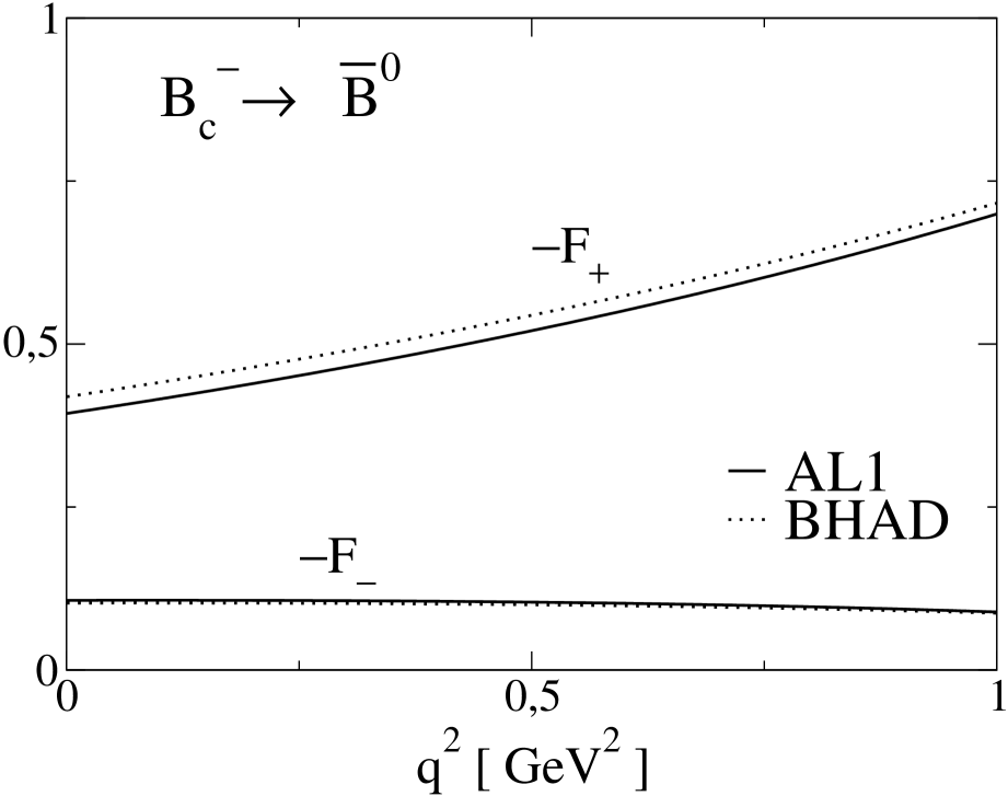
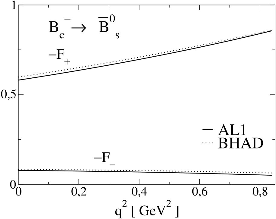
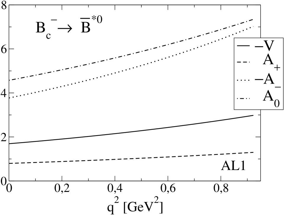
Figure 4.10: $F_{+}$ and $F_{-}$ form factors (solid lines) for $B_{c}^{-}\to\overline{B}^{0}$ and $B_{c}^{-}\to\overline{B}^{0}_{s}$ semileptonic decay, and $V$ (solid line), $A_{+}$ (dashed line), $A_{-}$ (dotted line) and $A_{0}$ (dashed–dotted line) form factors for $B_{c}^{-}\to\overline{B}^{*0}$ and $B_{c}^{-}\to\overline{B}^{*0}_{s}$ semileptonic decays evaluated with the AL1 potential. For the first two cases, and for comparison, we also show with dotted lines the results obtained with the Bhaduri (BHAD) potential.

In Table 4.14 we show $F_{+}$, $F_{-}$ and $F_{0}$ (defined as in Eq. (4.11) changing the mass of the final meson) of the $B_{c}^{-}\to\overline{B}^{0},\,\overline{B}^{0}_{s}$ transitions evaluated at $q^{2}_{min}$ and $q^{2}_{max}$ and compare them with the results by Ivanov et al. [164] and Ebert et al. [166]. Notice that, to favor comparison, we have changed the signs of the form factors by Ebert et al. (they evaluate $B_{c}^{+}$ decay) in accordance with the results in appendix E.2. The agreement with the results by Ebert et al. is good. We also agree with Ivanov et al. for $F_{+}$, but get very different results for $F_{-}$. As fermion masses are very small the disagreement in the $F_{-}$ form factor will have a negligible effect on the decay width.

$B_{c}^{-}\to\overline{B}^{0}\,l^{-}\bar{\nu}_{l}\ \$	$q^{2}_{\mathrm{min}}$	$q^{2}_{\mathrm{max}}$	$B_{c}^{-}\to\overline{B}^{0}_{s}\,l^{-}\bar{\nu}_{l}\ \$	$q^{2}_{\mathrm{min}}$	$q^{2}_{\mathrm{max}}$
$F_{+}$			$F_{+}$
This work	$-0.39^{+0.03}_{-0.03}$	$-0.70^{+0.004}_{-0.02}$	This work	$-0.58^{+0.01}_{-0.02}$	$-0.86^{+0.01}_{-0.01}$
[164]	$-0.58$	$-0.96$	[164]	$-0.61$	$-0.92$
[166]	$-0.39$	$-0.96$	[166]	$-0.50$	$-0.99$
$F_{-}$			$F_{-}$
This work	$-0.11^{+0.02}_{-0.03}$	$-0.09^{+0.01}_{-0.06}$	This work	$-0.08^{+0.01}_{-0.02}$	$-0.05^{+0.01}_{-0.03}$
[164]	2.14	2.98	[164]	1.83	2.35
$F_{0}$			$F_{0}$
This work	$-0.39^{+0.03}_{-0.03}$	$-0.71^{+0.05}_{-0.02}$	This work	$-0.58_{-0.02}$	$-0.86^{+0.01}_{-0.01}$
[166]	$-0.39$	$-0.80$	[166]	$-0.50$	$-0.86$

Table 4.14: $F_{+}$, $F_{-}$ and $F_{0}$ evaluated at $q^{2}_{\mathrm{min}}$ and $q^{2}_{\mathrm{max}}$ compared to the ones obtained by Ivanov et al. [164] and Ebert et al. [166]. Our central values have been obtained with the AL1 potential. Here $l$ stands for $l=e,\,\mu$.

In Table 4.15 we show $V$, $A_{+}$, $A_{-}$, $A_{0}$ and $\widetilde{A}_{0}$ (defined as in Eq. (4.15) changing the mass of the final meson) of the $B_{c}^{-}\to\overline{B}^{*0},\,\overline{B}^{*0}_{s}$ evaluated at $q^{2}_{min}$ and $q^{2}_{max}$ and compare them with the results by Ivanov et al. [164] and Ebert et al. [166]. With some exceptions the agreement with Ebert’s results is bad in this case. We are also in clear disagreement with Ivanov’s results.

$B_{c}^{-}\to\overline{B}^{*0}\,l^{-}\bar{\nu}_{l}\ \$	$q^{2}_{\mathrm{min}}$	$q^{2}_{\mathrm{max}}$	$B_{c}^{-}\to\overline{B}^{*0}_{s}\,l^{-}\bar{\nu}_{l}\ \$	$q^{2}_{\mathrm{min}}$	$q^{2}_{\mathrm{max}}$
$V$			$V$
This work	$-1.69^{+0.11}_{-0.09}$	$-2.98^{+0.17}_{-0.03}$	This work	$-2.29^{+0.02}_{-0.09}$	$-3.32^{+0.04}_{-0.01}$
[164]		$-5.32^{*}$	[164]		$-4.91^{*}$
[166]	$-3.94$	$-8.91$	[166]	$-3.44$	$-6.25$
$A_{+}$			$A_{+}$
This work	$-0.80^{+0.02}_{-0.02}$	$-1.30^{+0.02}$	This work	$-0.98^{+0.01}_{-0.03}$	$-1.35^{+0.03}_{-0.02}$
[164]		0.49	[164]		0.21
[166]	$-2.89$	$-2.83$	[166]	$-2.19$	$-2.62$
$A_{-}$			$A_{-}$
This work	$3.77^{+0.15}_{-0.17}$	$7.02_{-0.35}$	This work	$4.78^{+0.23}_{-0.01}$	$7.17^{+0.06}_{-0.18}$
[164]		18.0	[164]		15.9
$A_{0}$			$A_{0}$
This work	$-4.57^{+0.27}_{-0.33}$	$-7.34^{+0.28}_{-0.49}$	This work	$-7.39^{+0.14}_{-0.30}$	$-10.10^{+0.22}_{-0.16}$
[164]		$-5.07$	[164]		$-6.60$
[166]	$-5.08$	$-8.70$	[166]	$-6.60$	$-10.23$
$\widetilde{A}_{0}$			$\widetilde{A}_{0}$
This work	$-0.34^{+0.03}_{-0.03}$	$-0.60^{+0.05}_{-0.02}$	This work	$-0.51^{+0.01}_{-0.03}$	$-0.74^{+0.01}_{-0.01}$
[166]	$-0.20$	$-1.06$	[166]	$-0.35$	$-0.91$

Table 4.15: $V$, $A_{+}$, $A_{-}$, $A_{0}$ and $\widetilde{A}_{0}$ evaluated at $q^{2}_{\mathrm{min}}$ and $q^{2}_{\mathrm{max}}$ compared to the ones obtained by Ivanov et al. [164] and Ebert et al. [166]. Our central values have been obtained with the AL1 potential. Here $l$ stands for $l=e,\,\mu$. Asterisk as in Table 4.4.

4.5.2 Decay width

In Tables 4.16, 4.17 we give respectively our results for the partial helicity widths and forward-backward asymmetries.

$B^{-}_{c}\to$	$\Gamma_{U}$	$\widetilde{\Gamma}_{U}$	$\Gamma_{L}$	$\widetilde{\Gamma}_{L}$	$\Gamma_{P}$	$\widetilde{\Gamma}_{S}$	$\widetilde{\Gamma}_{SL}$
$\overline{B}^{0}\,e^{-}\bar{\nu}_{e}$	0	0	$0.65^{+0.07}_{-0.09}$	$0.14^{+0.02}_{-0.02}\ 10^{-5}$	0	$0.47^{+0.05}_{-0.07}\ 10^{-5}$	$0.15^{+0.01}_{-0.02}\ 10^{-5}$
$\overline{B}^{0}\,\mu^{-}\bar{\nu}_{\mu}$	0	0	$0.55^{+0.06}_{-0.07}$	$0.15^{+0.01}_{-0.02}\ 10^{-1}$	0	$0.64^{+0.16}_{-0.09}\ 10^{-1}$	$0.17^{+0.02}_{-0.02}\ 10^{-1}$
$\overline{B}_{s}^{0}\,e^{-}\bar{\nu}_{e}$	0	0	$15.1^{+0.7}_{-0.3}$	$0.43^{+0.02}_{-0.01}\ 10^{-4}$	0	$0.14^{+0.01}\ 10^{-3}$	$0.45^{+0.03}_{-0.01}\ 10^{-4}$
$\overline{B}_{s}^{0}\,\mu^{-}\bar{\nu}_{\mu}$	0	0	$12.4^{+0.5}_{-0.3}$	$0.40^{+0.02}_{-0.01}$	0	$1.69^{+0.08}_{-0.03}$	$0.47^{+0.02}_{-0.01}$
$\overline{B}^{*0}\,e^{-}\bar{\nu}_{e}$	$0.83^{+0.08}_{-0.11}$	$0.26^{+0.03}_{-0.04}\ 10^{-6}$	$0.76^{+0.09}_{-0.11}$	$0.10^{+0.02}_{-0.01}\ 10^{-5}$	$0.36_{-0.05}^{+0.03}$	$0.27^{+0.04}_{-0.05}\ 10^{-5}$	$0.96^{+0.15}_{-0.15}\ 10^{-6}$
$\overline{B}^{*0}\,\mu^{-}\bar{\nu}_{\mu}$	$0.79^{+0.10}_{-0.11}$	$0.97^{+0.11}_{-0.13}\ 10^{-2}$	$0.68^{+0.08}_{-0.10}$	$0.14^{+0.01}_{-0.03}\ 10^{-1}$	$0.34_{-0.05}^{+0.02}$	$0.28^{+0.04}_{-0.05}\ 10^{-1}$	$0.11^{+0.02}_{-0.02}\ 10^{-1}$
$\overline{B}_{s}^{*0}\,e^{-}\bar{\nu}_{e}$	$16.7^{+0.8}_{-0.7}$	$0.66^{+0.04}_{-0.03}\ 10^{-5}$	$16.8^{+1.1}_{-0.8}$	$0.33^{+0.02}_{-0.02}\ 10^{-4}$	$6.11_{-0.20}^{+0.21}$	$0.88^{+0.08}_{-0.05}\ 10^{-4}$	$0.30^{+0.03}_{-0.01}\ 10^{-4}$
$\overline{B}_{s}^{*0}\,\mu^{-}\bar{\nu}_{\mu}$	$15.6^{+0.8}_{-0.6}$	$0.24^{+0.02}_{-0.01}$	$14.5^{+1.0}_{-0.6}$	$0.37^{+0.02}_{-0.02}$	$5.66_{-0.19}^{+0.18}$	$0.77^{+0.06}_{-0.04}$	$0.30^{+0.02}_{-0.01}$

Table 4.16: Partial helicity widths in units of $10^{-15}$ GeV for $B_{c}^{-}$ decay. Central values have been evaluated with the AL1 potential.

	$A_{FB}(e)$	$A_{FB}(\mu)$
$B_{c}^{-}\to\overline{B}^{0}$	$0.67^{+0.02}\ 10^{-5}$	$0.82^{+0.01}\ 10^{-1}$
$B_{c}^{-}\to\overline{B}_{s}^{0}$	$0.89^{+0.01}\ 10^{-5}$	$0.96^{+0.01}\ 10^{-1}$
$B_{c}^{-}\to\overline{B}^{*0}$	$0.17_{-0.01}$	$0.19_{-0.01}$
$B_{c}^{-}\to\overline{B}_{s}^{*0}$	$0.14_{-0.01}$	$0.16^{+0.01}$

Table 4.17: Forward-backward asymmetry. Our central values have been evaluated with the AL1 potential. We would obtain the same results for $B_{c}^{+}\to B^{0}$ decays.

In Fig. 4.11 we show the differential decay width for the $B_{c}^{-}\to\overline{B}^{0}\,l^{-}\bar{\nu}_{l}$, $B_{c}^{-}\to\overline{B}^{0}_{s}\,l^{-}\bar{\nu}_{l}$, $B_{c}^{-}\to\overline{B}^{*0}\,l^{-}\bar{\nu}_{l}$ and $B_{c}^{-}\to\overline{B}^{*0}_{s}\,l^{-}\bar{\nu}_{l}$ transitions ($l=e,\,\mu$). In Tables 4.18, 4.19 we give the total decay widths and branching ratios and compare them with determinations by other groups. Our results are in better agreement with the ones obtained by Ebert et al. [166], Colangelo et al. [176], Anisimov et al. [177] and Lu et al. [181].

	$\Gamma\ [10^{-15}\ \mathrm{GeV}]$
	This work	[164]	[166]	[167]	[170]	[171]	[174]	[176]	[177]	[178]	[181]
$B^{-}_{c}\to\overline{B}^{0}\,e\,\bar{\nu}_{e}$	$0.65^{+0.07}_{-0.09}$	2.1	0.6	2.30	1.14	1.90	4.9	0.9(1.0)			0.59
$B^{-}_{c}\to\overline{B}^{0}\,\mu\,\bar{\nu}_{\mu}$	$0.63^{+0.07}_{-0.09}$
$B^{-}_{c}\to\overline{B}_{s}^{0}\,e\,\bar{\nu}_{e}$	$15.1^{+0.7}_{-0.3}$	29	12	26.6	14.3	26.8	59	11.1(12.9)	15	12.3	11.75
$B^{-}_{c}\to\overline{B}_{s}^{0}\,\mu\,\bar{\nu}_{\mu}$	$14.5^{+0.6}_{-0.3}$
$B^{-}_{c}\to\overline{B}^{*0}\,e\,\bar{\nu}_{e}$	$1.59^{+0.17}_{-0.22}$	2.3	1.7	3.32	3.53	2.34	8.5	2.8(3.2)			2.44
$B^{-}_{c}\to\overline{B}^{*0}\,\mu\,\bar{\nu}_{\mu}$	$1.52^{+0.17}_{-0.21}$
$B^{-}_{c}\to\overline{B}_{s}^{*0}\,e\,\bar{\nu}_{e}$	$33.5^{+1.9}_{-1.5}$	37	25	44.0	50.4	34.6	65	33.5(37.0)	34	19.0	32.56
$B^{-}_{c}\to\overline{B}_{s}^{*0}\,\mu\,\bar{\nu}_{\mu}$	$31.5^{+1.8}_{-1.4}$

Table 4.18: Decay widths in units of $10^{-15}$ GeV. Our central values have been evaluated with the AL1 potential.

	B.R. (%)
	This work	[162]	[166]	[167]	[170]	[174]	[176]	[177]	[178]
$B^{-}_{c}\to\overline{B}^{0}\,e\,\bar{\nu}_{e}$	$0.046^{+0.004}_{-0.007}$	0.071	0.042	0.16	0.078	0.34	0.06		0.048
$B^{-}_{c}\to\overline{B}^{0}\,\mu\,\bar{\nu}_{\mu}$	$0.044^{+0.005}_{-0.006}$
$B^{-}_{c}\to\overline{B}_{s}^{0}\,e\,\bar{\nu}_{e}$	$1.06^{+0.05}_{-0.02}$	1.10	0.84	1.82	0.98	4.03	0.8	0.99	0.92
$B^{-}_{c}\to\overline{B}_{s}^{0}\,\mu\,\bar{\nu}_{\mu}$	$1.02^{+0.04}_{-0.02}$
$B^{-}_{c}\to\overline{B}^{*0}\,e\,\bar{\nu}_{e}$	$0.11^{+0.01}_{-0.01}$	0.063	0.12	0.23	0.24	0.58	0.19		0.051
$B^{-}_{c}\to\overline{B}^{*0}\,\mu\,\bar{\nu}_{\mu}$	$0.11^{+0.01}_{-0.02}$
$B^{-}_{c}\to\overline{B}_{s}^{*0}\,e\,\bar{\nu}_{e}$	$2.35^{+0.14}_{-0.10}$	2.37	1.75	3.01	3.45	5.06	2.3	2.30	1.41
$B^{-}_{c}\to\overline{B}_{s}^{*0}\,\mu\,\bar{\nu}_{\mu}$	$2.22^{+0.12}_{-0.10}$

Table 4.19: Branching ratios in % . Our central values have been evaluated with the AL1 potential.

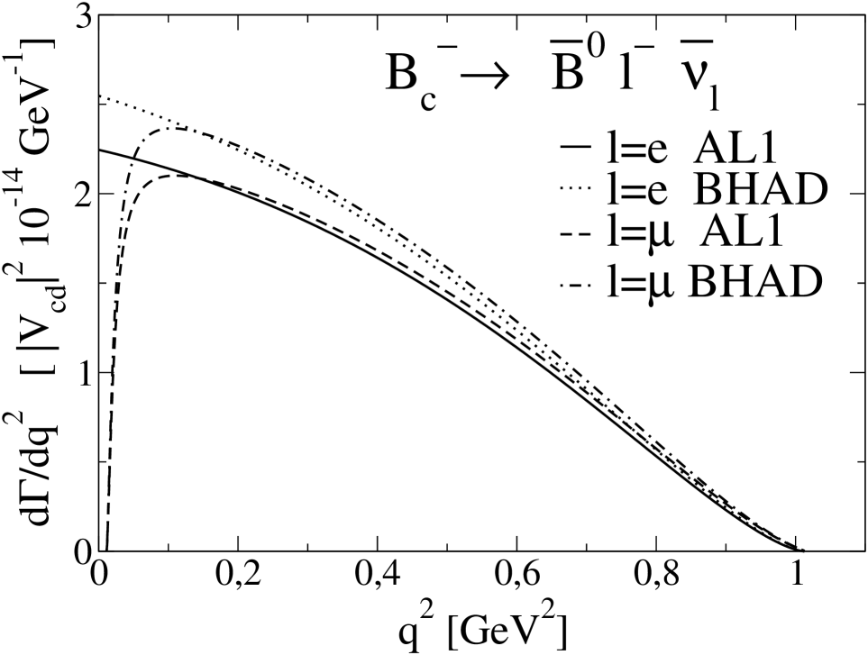
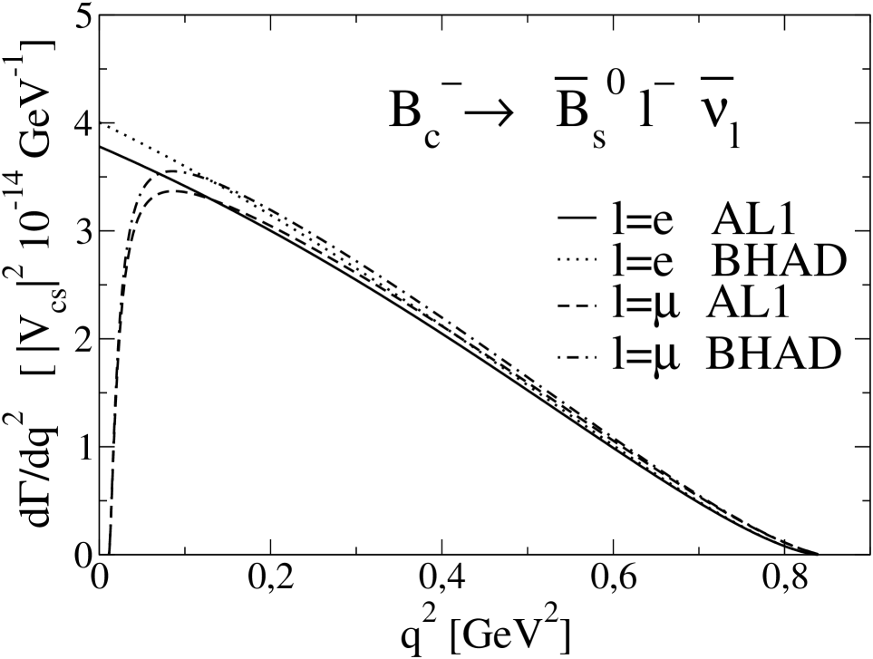
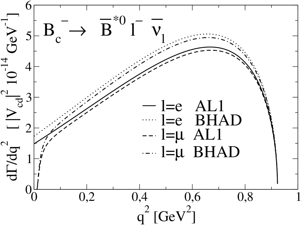
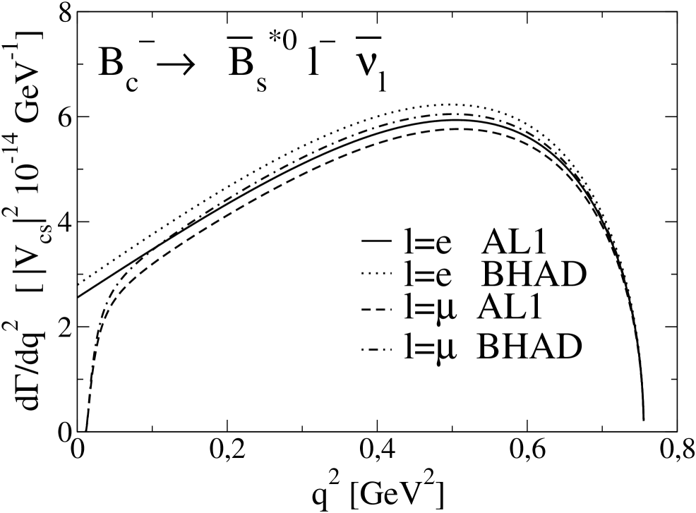
Figure 4.11: Differential decay width for the for the $B_{c}^{-}\to\overline{B}^{0}\,l^{-}\bar{\nu}_{l}$ and $B_{c}^{-}\to\overline{B}^{0}_{s}\,l^{-}\bar{\nu}_{l}$, $B_{c}^{-}\to\overline{B}^{*0}\,l^{-}\bar{\nu}_{l}$ and $B_{c}^{-}\to\overline{B}^{*0}_{s}\,l^{-}\bar{\nu}_{l}$ ($l=e,\,\mu$) transitions. Solid line: results for a final $e$ evaluated with the AL1 potential; dotted line: results for a final $e$ evaluated with the Bhaduri (BHAD) potential; dashed line: results for a final $\mu$ evaluated with the AL1 potential; dashed–dotted line: results for a final $\mu$ evaluated with the Bhaduri (BHAD) potential.

4.5.3 Heavy quark spin symmetry

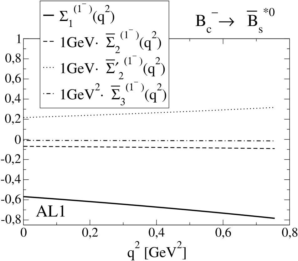
Figure 4.12: $\Sigma_{1}^{(0^{-})}$ (solid line) and $\Sigma_{2}^{(0^{-})}$ (dashed line) of the $B_{c}^{-}\to\overline{B}^{0}$ and $B_{c}^{-}\to\overline{B}^{0}_{s}$ transitions, and $\Sigma_{1}^{(1^{-})}$ (solid line), $\overline{\Sigma}_{2}^{(1^{-})}$ (dashed line), $\overline{\Sigma}_{2}^{\prime(1^{-})}$ (dotted line) and $\overline{\Sigma}_{3}^{(1^{-})}$ (dashed dotted line) of the $B_{c}^{-}\to\overline{B}^{*0}$ and $B_{c}^{-}\to\overline{B}^{*0}_{s}$ transitions evaluated with the AL1 potential.

In Fig. 4.12 we give $\Sigma_{1}^{(0^{-})}$ and $\Sigma_{2}^{(0^{-})}$ of the $B_{c}^{-}\to\overline{B}^{0}$ and $B_{c}^{-}\to\overline{B}^{0}_{s}$ transitions, and $\Sigma_{1}^{(1^{-})}$, $\overline{\Sigma}_{2}^{(1^{-})}$, $\overline{\Sigma}_{2}^{\prime(1^{-})}$ and $\overline{\Sigma}_{3}^{(1^{-})}$ of the $B_{c}^{-}\to\overline{B}^{*0}$ and $B_{c}^{-}\to\overline{B}^{*0}_{s}$ transitions.

We can take the infinite heavy quark mass limit on our analytic expressions with the result that near zero recoil

$$\Sigma_{1}^{(1^{-})} = \Sigma_{1}^{(0^{-})}$$

$$\overline{\Sigma}_{2}^{(1^{-})} = \overline{\Sigma}_{2}^{\prime(1^{-})}=-\overline{\Sigma}_{2}^{(0^{-})}$$

$$\overline{\Sigma}_{3}^{(1^{-})} = 0$$ (4.63)

When compared to the results of HQSS by Jenkins et al. [72] we see differences. In Ref. [72] we find $\overline{\Sigma}_{2}^{(1^{-})}=\overline{\Sigma}_{2}^{(0^{-})}$ instead. This is wrong as there is a misprint in Ref. [72] that has not been noted before: the sign of the term in $v^{\mu}$ in the last expression of Eqs. (2.9) and (2.10) in Ref. [72] should be a minus [190]. Also from Ref. [72] one would expect $\overline{\Sigma}_{2}^{\prime(1^{-})}=\overline{\Sigma}_{2}^{(0^{-})}$ contradicting our result in Eq. (4.5.3) were we find $\overline{\Sigma}_{2}^{\prime(1^{-})}=-\overline{\Sigma}_{2}^{(0^{-})}$. Our result is a clear prediction of the quark model and comes from the extra signs that appear due to the fact that it is the antiquark that decays (See appendix E.2). This difference between quark and antiquark decay was not properly reflected in their published work [190].

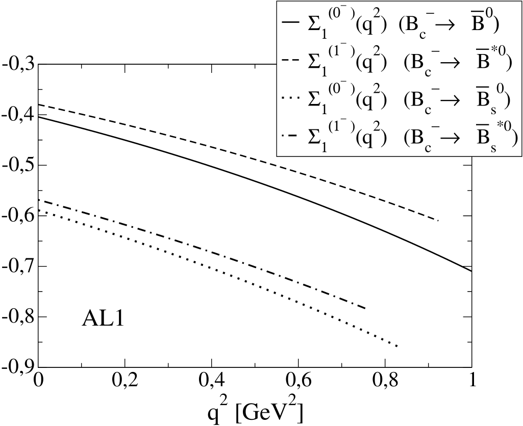
Figure 4.13: $\Sigma_{1}^{(0^{-})}$ of the semileptonic $B_{c}^{-}\to\overline{B}^{0}$ (solid line) and $B_{c}^{-}\to\overline{B}_{s}^{0}$ (dotted line) transitions, and $\Sigma_{1}^{(1^{-})}$ of the semileptonic $B_{c}^{-}\to\overline{B}^{*0}$ (dashed line) and $B_{c}^{-}\to\overline{B}_{s}^{*0}$ (dashed–dotted line) transitions evaluated with the AL1 potential.

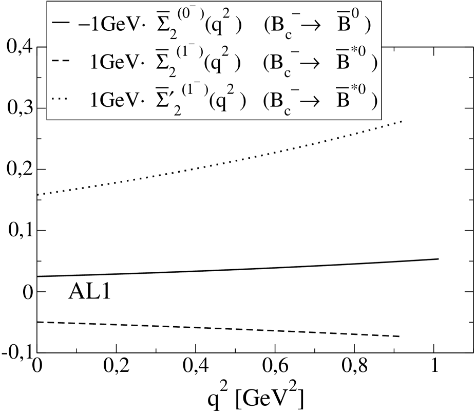
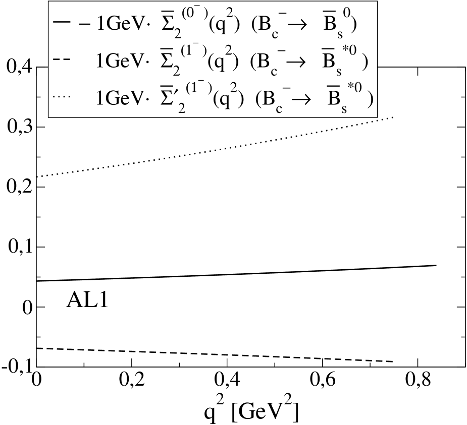
Figure 4.14: $-\overline{\Sigma}_{2}^{(0^{-})}$ (solid line) of the semileptonic $B_{c}^{-}\to\overline{B}^{0}$ and $B_{c}^{-}\to\overline{B}_{s}^{0}$ transitions, and $\overline{\Sigma}_{2}^{(1^{-})}$ (dashed line), $\overline{\Sigma}_{2}^{\prime(1^{-})}$ (dotted line) of the semileptonic $B_{c}^{-}\to\overline{B}^{*0}$ and $B_{c}^{-}\to\overline{B}_{s}^{*0}$ transitions evaluated with the AL1 potential.

How far are we from the infinite heavy quark mass limit? In Fig. 4.13 we show $\Sigma_{1}^{(0^{-})}$ of the semileptonic $B_{c}^{-}\to\overline{B}^{0}$ and $B_{c}^{-}\to\overline{B}_{s}^{0}$ transitions, and $\Sigma_{1}^{(1^{-})}$ of the semileptonic $B_{c}^{-}\to\overline{B}^{*0}$ and $B_{c}^{-}\to\overline{B}_{s}^{*0}$ transitions. The differences between the corresponding $\Sigma_{1}^{(0^{-})}$ and $\Sigma_{1}^{(1^{-})}$ are at the level of 10%. The differences are much more significant for $\overline{\Sigma}_{2}^{(0^{-})}$, $\overline{\Sigma}_{2}^{(1^{-})}$ and $\overline{\Sigma}_{2}^{\prime(1^{-})}$ that we show in Fig. 4.14. In each case the three curves shown would be the same in the infinite heavy quark mass limit. Clearly in this case corrections on the inverse of the heavy quark masses seem to be important.

4.6 Nonleptonic $B_{c}^{-}\to{B}\,M_{F}$ two-meson decays

In this section we will evaluate decay widths for nonleptonic $B_{c}^{-}\to{B}\ M_{F}$ two–meson decays where $M_{F}$ is a pseudoscalar or vector meson with no $b$ quark content, and, at this point, ${B}$ represents a meson with a $b$ quark. These decay modes involve a $\bar{c}\to\bar{d}$ or $\bar{c}\to\bar{s}$ transition at the quark level and they are governed, neglecting penguin operators, by the effective Hamiltonian  [162, 166]

$$H_{eff.}=\frac{G_{F}}{\sqrt{2}}\,\left\{V_{cd}\left[c_{1}(\mu)\,Q_{1}^{cd}+c_{2}(\mu)\,Q_{2}^{cd}\right]+V_{cs}\left[c_{1}(\mu)\,Q_{1}^{cs}+c_{2}(\mu)\,Q_{2}^{cs}\right]+H.c.\right\}$$

where $c_{1},\,c_{2}$ are scale–dependent Wilson coefficients, and $Q_{1}^{cd},\,Q_{2}^{cd},\,Q_{1}^{cs},\,Q_{2}^{cs}$ are local four–quark operators given by

$$Q_{1}^{cd} = \overline{\Psi}_{c}(0)\gamma_{\mu}(I-\gamma_{5})\Psi_{d}(0)\,\bigg{[}\ V_{ud}^{*}\,\overline{\Psi}_{d}(0)\gamma^{\mu}(I-\gamma_{5})\Psi_{u}(0)+V_{us}^{*}\,\overline{\Psi}_{s}(0)\gamma^{\mu}(I-\gamma_{5})\Psi_{u}(0)\bigg{]}$$

$$Q_{2}^{cd} = \overline{\Psi}_{c}(0)\gamma_{\mu}(I-\gamma_{5})\Psi_{u}(0)\,\bigg{[}\ V_{ud}^{*}\,\overline{\Psi}_{d}(0)\gamma^{\mu}(I-\gamma_{5})\Psi_{d}(0)+V_{us}^{*}\,\overline{\Psi}_{s}(0)\gamma^{\mu}(I-\gamma_{5})\Psi_{d}(0)\bigg{]}$$

$$Q_{1}^{cs} = \overline{\Psi}_{c}(0)\gamma_{\mu}(I-\gamma_{5})\Psi_{s}(0)\,\bigg{[}\ V_{ud}^{*}\,\overline{\Psi}_{d}(0)\gamma^{\mu}(I-\gamma_{5})\Psi_{u}(0)+V_{us}^{*}\,\overline{\Psi}_{s}(0)\gamma^{\mu}(I-\gamma_{5})\Psi_{u}(0)\bigg{]}$$

$$Q_{2}^{cs} = \overline{\Psi}_{c}(0)\gamma_{\mu}(I-\gamma_{5})\Psi_{u}(0)\,\bigg{[}\ V_{ud}^{*}\,\overline{\Psi}_{d}(0)\gamma^{\mu}(I-\gamma_{5})\Psi_{s}(0)+V_{us}^{*}\,\overline{\Psi}_{s}(0)\gamma^{\mu}(I-\gamma_{5})\Psi_{s}(0)\,\bigg{]}$$

We shall work again in the factorization approximation taking into account the Fierz reordered contribution so that the relevant coefficients are not $c_{1}$ and $c_{2}$ but the combinations

$$a_{1}(\mu)=c_{1}(\mu)+\frac{1}{N_{C}}\,c_{2}(\mu)\hskip 14.22636pt;\hskip 14.22636pta_{2}(\mu)=c_{2}(\mu)+\frac{1}{N_{C}}\,c_{1}(\mu)$$ (4.66)

The energy scale $\mu$ appropriate in this case is $\mu\simeq m_{c}$ and the values for $a_{1}$ and $a_{2}$ that we use are [162]

$$a_{1}=1.20\hskip 14.22636pt;\hskip 14.22636pta_{2}=-0.317$$ (4.67)

$\bullet$ $M_{F}=\pi^{-},\,\rho^{-},\,K^{-},\,K^{*-}$

	$\Gamma$ [$10^{-15}$ GeV]
	This work
$B_{c}^{-}\to\overline{B}^{0}\,\pi^{-}$	$1.10^{+0.14}_{-0.16}\,a_{1}^{2}$
$B_{c}^{-}\to\overline{B}^{0}\,\rho^{-}$	$1.41^{+0.12}_{-0.19}\,a_{1}^{2}$
$B_{c}^{-}\to\overline{B}^{0}\,K^{-}$	$0.098^{+0.012}_{-0.012}\,a_{1}^{2}$
$B_{c}^{-}\to\overline{B}^{0}\,K^{*-}$	$0.038^{+0.003}_{-0.005}\,a_{1}^{2}$
$B_{c}^{-}\to\overline{B}^{*0}\,\pi^{-}$	$0.71^{+0.12}_{-0.11}\,a_{1}^{2}$
$B_{c}^{-}\to\overline{B}^{*0}\,\rho^{-}$	$5.68^{+0.55}_{-0.77}\,1a_{1}^{2}$
$B_{c}^{-}\to\overline{B}^{*0}\,K^{-}$	$0.047^{+0.007}_{-0.007}\,a_{1}^{2}$
$B_{c}^{-}\to\overline{B}^{*0}\,K^{*-}$	$0.29^{+0.03}_{-0.04}\,a_{1}^{2}$
$B_{c}^{-}\to\overline{B}_{s}^{0}\,\pi^{-}$	$34.7^{+2.0}_{-0.6}\,a_{1}^{2}$
$B_{c}^{-}\to\overline{B}_{s}^{0}\,\rho^{-}$	$23.1^{+0.5}_{-0.6}\,a_{1}^{2}$
$B_{c}^{-}\to\overline{B}_{s}^{0}\,K^{-}$	$2.87^{+0.13}_{-0.06}\,a_{1}^{2}$
$B_{c}^{-}\to\overline{B}_{s}^{0}\,K^{*-}$	$0.13_{-0.01}\,a_{1}^{2}$
$B_{c}^{-}\to\overline{B}_{s}^{*0}\,\pi^{-}$	$22.8^{+2.2}_{-1.0}\,a_{1}^{2}$
$B_{c}^{-}\to\overline{B}_{s}^{*0}\,\rho^{-}$	$132^{+5}_{-6}\,a_{1}^{2}$
$B_{c}^{-}\to\overline{B}_{s}^{*0}\,K^{-}$	$1.29^{+0.10}_{-0.06}\,a_{1}^{2}$

	B.R. in %
	This work	[162]	[166]	[167]	[170]	[174]	[176]	[177]
$B_{c}^{-}\to\overline{B}^{0}\,\pi^{-}$	$0.11^{+0.01}_{-0.01}$	0.20	0.10	0.32	0.10	1.06	0.19	0.15
$B_{c}^{-}\to\overline{B}^{0}\,\rho^{-}$	$0.14^{+0.02}_{-0.02}$	0.20	0.13	0.59	0.28	0.96	0.15	0.19
$B_{c}^{-}\to\overline{B}^{0}\,K^{-}$	$0.010^{+0.001}_{-0.001}$	0.015	0.009	0.025	0.010	0.07	0.014
$B_{c}^{-}\to\overline{B}^{0}\,K^{*-}$	$0.0039^{+0.0003}_{-0.0005}$	0.0048	0.004	0.018	0.012	0.015	0.003
$B_{c}^{-}\to\overline{B}^{*0}\,\pi^{-}$	$0.072^{+0.012}_{-0.012}$	0.057	0.026	0.29	0.076	0.95	0.24	0.077
$B_{c}^{-}\to\overline{B}^{*0}\,\rho^{-}$	$0.58^{+0.05}_{-0.08}$	0.30	0.67	1.17	0.89	2.57	0.85	0.67
$B_{c}^{-}\to\overline{B}^{*0}\,K^{-}$	$0.0048^{+0.0007}_{-0.0008}$	0.0036	0.004	0.019	0.006	0.055	0.012
$B_{c}^{-}\to\overline{B}^{*0}\,K^{*-}$	$0.030^{+0.002}_{-0.004}$	0.013	0.032	0.037	0.065	0.058	0.033
$B_{c}^{-}\to\overline{B}_{s}^{0}\,\pi^{-}$	$3.51^{+0.19}_{-0.06}$	3.9	2.46	5.75	1.56	16.4	3.01	3.42
$B_{c}^{-}\to\overline{B}_{s}^{0}\,\rho^{-}$	$2.34^{+0.05}_{-0.06}$	2.3	1.38	4.41	3.86	7.2	1.34	2.33
$B_{c}^{-}\to\overline{B}_{s}^{0}\,K^{-}$	$0.29^{+0.01}_{-0.01}$	0.29	0.21	0.41	0.17	1.06	0.21
$B_{c}^{-}\to\overline{B}_{s}^{0}\,K^{*-}$	$0.013_{-0.001}$	0.011	0.0030		0.10		0.0043
$B_{c}^{-}\to\overline{B}_{s}^{*0}\,\pi^{-}$	$2.34^{+0.19}_{-0.14}$	2.1	1.58	5.08	1.23	6.5	3.50	1.95
$B_{c}^{-}\to\overline{B}_{s}^{*0}\,\rho^{-}$	$13.4^{+0.5}_{-0.6}$	11	10.8	14.8	16.8	20.2	10.8	12.1
$B_{c}^{-}\to\overline{B}_{s}^{*0}\,K^{-}$	$0.13^{+0.01}_{-0.01}$	0.13	0.11	0.29	0.13	0.37	0.16

Table 4.20: Decay widths in units of $10^{-15}$ GeV, and for general values of the Wilson coefficient $a_{1}$, and branching ratios in % for exclusive nonleptonic decays of the $B_{c}^{-}$ meson. Our central values have been obtained with the AL1 potential.

In this case $B$ denotes one of the $\overline{B}^{0},\,\overline{B}^{*0},\,\overline{B}_{s}^{0},\,\overline{B}_{s}^{*0}$. The decay widths are

$$M_{F}\equiv 0^{-}\ \mathrm{case}$$

$$\Gamma=\frac{G_{F}^{2}}{16\pi m^{2}_{B_{c}}}\,|V_{cd}|^{2}\,|V_{F}|^{2}\ a_{1}^{2}\,\frac{\lambda^{1/2}(m^{2}_{B_{c}},\,m^{2}_{\overline{B}^{0},\,\overline{B}^{*0}},\,m^{2}_{F})}{2m_{B_{c}}}\,m_{F}^{2}\,f^{2}_{F}\,{\cal H}_{tt}^{B_{c}^{-}\to\overline{B}^{0},\,\overline{B}^{*0}}(m_{F}^{2})$$

$$M_{F}\equiv 1^{-}\ \mathrm{case}$$

$$\Gamma=\frac{G_{F}^{2}}{16\pi m^{2}_{B_{c}}}\,|V_{cd}|^{2}\,|V_{F}|^{2}\ a_{1}^{2}\ \frac{\lambda^{1/2}(m^{2}_{B_{c}},\,m^{2}_{\overline{B}^{0},\,\overline{B}^{*0}},\,m^{2}_{F})}{2m_{B_{c}}}\,m_{F}^{2}\,f^{2}_{F}$$

$$\hskip 56.9055pt\times\left({\cal H}_{+1+1}^{B_{c}^{-}\to\overline{B}^{0},\,\overline{B}^{*0}}(m_{F}^{2})+{\cal H}_{-1-1}^{B_{c}^{-}\to\overline{B}^{0},\,\overline{B}^{*0}}(m_{F}^{2})+{\cal H}_{00}^{B_{c}^{-}\to\overline{B}^{0},\,\overline{B}^{*0}}(m_{F}^{2})\right)$$

(4.68)

and similarly for $\overline{B}^{0}_{s},\,\overline{B}^{*0}_{s}$ with $|V_{cd}|\to|V_{cs}|;\,\overline{B}^{0},\,\overline{B}^{*0}\to\overline{B}^{0}_{s},\,\overline{B}^{*0}_{s}$. $V_{F}=V_{ud}$ or $V_{F}=V_{us}$ depending on whether $M_{F}=\pi^{-},\,\rho^{-}$ or $M_{F}=K^{-},\,K^{*-}$, $f_{F}$ is the decay constant of the $M_{F}$ meson, and the different ${\cal H}_{rr}$ have been evaluated at $q^{2}=m_{F}^{2}$. In Table 4.20 we show the decay widths for a general value of the Wilson coefficient $a_{1}$, and the corresponding branching ratios evaluated with $a_{1}=1.20$. The transition $B_{c}^{-}\to\overline{B}^{*0}_{s}K^{*-}$ is not allowed with the new $B_{c}$ mass value from Ref. [182]. Our branching ratios for a final $\overline{B}^{0}_{s}$ or $\overline{B}^{*0}_{s}$ are in very good agreement with the results by Ivanov et al. [162], while for a final $\overline{B}^{0}$ or $\overline{B}^{*0}$ we are in very good agreement with the results by Ebert et al. [166] (with the exception of the $B_{c}\to\overline{B}^{*0}\pi^{-}$ decay).

$\bullet$$M_{F}=\pi^{0},\,\rho^{0},\,K^{0},\,K^{*0}$

Here the generic name ${B}$ stands for a ${B}^{-}$ or a ${B}^{*-}$ meson. The different decay widths are given by

$$M_{F}\equiv 0^{-}\ \mathrm{case}$$

$$\Gamma=\frac{G_{F}^{2}}{16\pi m^{2}_{B_{c}}}\,|V_{ud}|^{2}\,|V_{F}|^{2}\ a_{2}^{2}\,\frac{\lambda^{1/2}(m^{2}_{B_{c}},\,m^{2}_{B^{-},\,B^{*-}},\,m^{2}_{F})}{2m_{B_{c}}}\,m_{F}^{2}\,\widetilde{f}^{2}_{F}\,{\cal H}_{tt}^{B_{c}^{-}\to{B}^{-},\,{B}^{*-}}(m_{F}^{2})$$

$$M_{F}\equiv 1^{-}\ \mathrm{case}$$

$$\Gamma=\frac{G_{F}^{2}}{16\pi m^{2}_{B_{c}}}\,|V_{ud}|^{2}\,|V_{F}|^{2}\ a_{2}^{2}\ \frac{\lambda^{1/2}(m^{2}_{B_{c}},\,m^{2}_{{B}^{-},\,{B}^{*-}},\,m^{2}_{F})}{2m_{B_{c}}}\,m_{F}^{2}\,\widetilde{f}^{2}_{F}$$

$$\hskip 56.9055pt\times\left({\cal H}_{+1+1}^{B_{c}^{-}\to{B}^{-},\,{B}^{*-}}(m_{F}^{2})+{\cal H}_{-1-1}^{B_{c}^{-}\to{B}^{-},\,{B}^{*-}}(m_{F}^{2})+{\cal H}_{00}^{B_{c}^{-}\to{B}^{-},\,{B}^{*-}}(m_{F}^{2})\right)$$

(4.69)

where $V_{F}=V_{cd}$ or $V_{F}=V_{cs}$ depending on whether $M_{F}=\pi^{0},\,\rho^{0}$ or $M_{F}=K^{0},\,K^{*0}$, $\widetilde{f}_{F}=f_{F}$ for $M_{F}=K^{0},\,K^{*0}$ whereas $\widetilde{f}_{F}=f_{F}/\sqrt{2}$ for $M_{F}=\pi^{0},\,\rho^{0}$, with $f_{F}$ the $M_{F}$ meson decay constant, and the different ${\cal H}_{rr}$ evaluated at $q^{2}=m_{F}^{2}$. The latter have been obtained from the matrix elements for the effective current operator $\overline{\Psi}_{c}(0)\gamma^{\mu}(I-\gamma_{5})\Psi_{u}(0)$. The decay widths, for a general value of the Wilson coefficient $a_{2}$, and the corresponding branching ratios are shown in Table 4.21. With the exception of the $B_{c}^{-}\to B^{*-}\pi^{0}$ case, our results are in a global good agreement with the ones by Ebert et al. [166].

	$\Gamma$ [$10^{-15}$ GeV]
	This work
$B_{c}^{-}\to{B}^{-}\,\pi^{0}$	$0.54^{+0.07}_{-0.07}\,a_{2}^{2}$
$B_{c}^{-}\to{B}^{-}\,\rho^{0}$	$0.71^{+0.06}_{-0.10}\,a_{2}^{2}$
$B_{c}^{-}\to{B}^{-}\,K^{0}$	$35.3^{+4.0}_{-4.9}\,a_{2}^{2}$
$B_{c}^{-}\to{B}^{-}\,K^{*0}$	$13.1^{+0.9}_{-0.7}\,a_{2}^{2}$
$B_{c}\to{B}^{*-}\,\pi^{0}$	$0.35^{+0.06}_{-0.05}\,a_{2}^{2}$
$B_{c}\to{B}^{*-}\,\rho^{0}$	$2.84^{+0.27}_{-0.39}\,a_{2}^{2}$
$B_{c}\to{B}^{*-}\,K^{0}$	$16.9^{+2.4}_{-2.7}\,a_{2}^{2}$
$B_{c}\to{B}^{*-}\,K^{*0}$	$103^{+8}_{-13}\,a_{2}^{2}$

	B.R. in %
	This work	[162]	[166]	[167]	[170]	[174]	[177]
$B_{c}^{-}\to{B}^{-}\,\pi^{0}$	$0.0038^{+0.0005}_{-0.0006}$	0.007	0.004	0.011	0.004	0.037	0.007
$B_{c}^{-}\to{B}^{-}\,\rho^{0}$	$0.0050^{+0.0004}_{-0.0007}$	0.0071	0.005	0.020	0.010	0.034	0.009
$B_{c}^{-}\to{B}^{-}\,K^{0}$	$0.25^{+0.03}_{-0.04}$	0.38	0.24	0.66	0.27	1.98	0.17
$B_{c}^{-}\to{B}^{-}\,K^{*0}$	$0.093^{+0.006}_{-0.013}$	0.11	0.09	0.47	0.32	0.43	0.095
$B_{c}\to{B}^{*-}\,\pi^{0}$	$0.0025^{+0.0004}_{-0.0005}$	0.0020	0.001	0.010	0.003	0.033	0.004
$B_{c}\to{B}^{*-}\,\rho^{0}$	$0.020^{+0.002}_{-0.003}$	0.011	0.024	0.041	0.031	0.09	0.031
$B_{c}\to{B}^{*-}\,K^{0}$	$0.12^{+0.02}_{-0.02}$	0.088	0.11	0.50	0.16	1.60	0.061
$B_{c}\to{B}^{*-}\,K^{*0}$	$0.73^{+0.06}_{-0.10}$	0.32	0.84	0.97	1.70	1.67	0.57

Table 4.21: Decay widths in units of $10^{-15}$ GeV, and for general values of the Wilson coefficient $a_{2}$, and branching ratios in % for exclusive nonleptonic decays of the $B_{c}^{-}$ meson. Our central values have been obtained with the AL1 potential.

Chapter 5 Doubly heavy baryons spectroscopy and static properties

5.1 Introduction

Baryon	$S$	$J^{P}$	$I$	$S_{h}^{\pi}$	Quark content
$\Xi_{cc}$	0	$\frac{1}{2}^{+}$	$\frac{1}{2}$	$1^{+}$	$ccl$
$\Xi^{*}_{cc}$	0	$\frac{3}{2}^{+}$	$\frac{1}{2}$	$1^{+}$	$ccl$
$\Omega_{cc}$	$-1$	$\frac{1}{2}^{+}$	0	$1^{+}$	$ccs$
$\Omega^{*}_{cc}$	$-1$	$\frac{3}{2}^{+}$	$0$	$1^{+}$	$ccs$
$\Xi_{bb}$	0	$\frac{1}{2}^{+}$	$\frac{1}{2}$	$1^{+}$	$bbl$
$\Xi^{*}_{bb}$	0	$\frac{3}{2}^{+}$	$\frac{1}{2}$	$1^{+}$	$bbl$
$\Omega_{bb}$	$-1$	$\frac{1}{2}^{+}$	0	$1^{+}$	$bbs$
$\Omega^{*}_{bb}$	$-1$	$\frac{3}{2}^{+}$	$0$	$1^{+}$	$bbs$
$\Xi^{\prime}_{bc}$	0	$\frac{1}{2}^{+}$	$\frac{1}{2}$	$0^{+}$	$bcl$
$\Xi_{bc}$	0	$\frac{1}{2}^{+}$	$\frac{1}{2}$	$1^{+}$	$bcl$
$\Xi^{*}_{bc}$	0	$\frac{3}{2}^{+}$	$\frac{1}{2}$	$1^{+}$	$bcl$
$\Omega^{\prime}_{bc}$	$-1$	$\frac{1}{2}^{+}$	0	$0^{+}$	$bcs$
$\Omega_{bc}$	$-1$	$\frac{1}{2}^{+}$	0	$1^{+}$	$bcs$
$\Omega^{*}_{bc}$	$-1$	$\frac{3}{2}^{+}$	$0$	$1^{+}$	$bcs$

Table 5.1: Quantum numbers of doubly heavy baryons analyzed in this study. $S$, $J^{P}$ are strangeness and the spin parity of the baryon, $I$ is the isospin, and $S_{h}^{\pi}$ is the spin parity of the heavy degrees of freedom. $l$ denotes a light $u$ or $d$ quark .

The subject of doubly heavy baryons has been attracting attention for a long time. Magnetic moments of doubly charmed baryons were evaluated back in the 70’s by Lichtenberg [191] within a nonrelativistic approach. The infinite heavy quark mass limit was already used in the 90’s to relate the spectrum of doubly heavy baryons to the one of mesons with a single heavy quark [192], or to analyze their semileptonic decay [193]. A factor of two error in the hyperfine splittings of Ref. [192] have been recently noticed by the potential nonrelativistic QCD (pNRQCD) calculation of Ref. [194].

On the experimental side the SELEX Collaboration claimed evidence for the $\Xi^{+}_{cc}$ baryon, in the $\Lambda_{c}^{+}K^{-}\pi^{+}$ and $pD^{+}K^{-}$ decay modes, with a mass of $M_{\Xi^{+}_{cc}}=3519\pm 1\ \mathrm{MeV/c^{2}}$ [195]. Those results were challenged by a theoretical analysis [196] which claimed the observed events by the SELEX Collaboration could be explained without the involvement of doubly charmed baryons. Other experimental collaborations like FOCUS [197], BABAR  [198] and BELLE [199] have found no evidence for doubly charmed baryons so far. At present the $\Xi^{+}_{cc}$ has only a one star status and it is not listed in the particle summary table [188].

As discussed before, for hadrons with two heavy quarks one can apply HQSS [72], which amounts to the decoupling of the heavy quark spins in the infinite heavy quark mass limit. In that limit one can consider the total spin of the two heavy quark subsystem ($S_{h}$) to be well defined. In this work we shall assume this is a good approximation for the actual heavy quark masses. This approximation, which is the only one related to the infinite heavy quark mass limit that we shall use, will certainly simplify the solution of the baryon three–quark problem. Recently the authors of Ref. [194] have developed and effective theory (pNRQCD) suitable to describe baryons with two and three heavy quarks.

Solving the three–body problem is not an easy task and here we shall do it by means of a variational approach. The approach, with obvious changes, was already applied with good results in the study of baryons with one heavy quark [200]. This method, that leads to simple and manageable wave functions, is made possible by the simplifications introduced in the problem by the fact that we can consider $S_{h}$ to be well defined.

Our simple variational calculation reproduces the results for static properties obtained in Ref. [75] by solving more involved Faddeev type equations. Our method has the advantage that we provide explicit and manageable wave functions that can be used to evaluate further observables. Static properties like masses and magnetic moments of doubly heavy baryons have also been studied in other models. Masses have been calculated in the relativistic quark model assuming a light quark heavy diquark structure [201], the potential approach and sum rules of QCD [202], the nonperturbative QCD approach [203], the Bethe–Salpeter equation applied to the light quark heavy diquark [204], the nonrelativistic quark model with harmonic oscillator potential [205] or with the use of QCD derived potentials [206, 207], the relativistic quasi–potential quark model [208], with the use of the Feynman-Hellman theorem and semi-empirical mass formulas within the framework of a nonrelativistic constituent quark model [209, 210], in effective field theories [65, 194], or in lattice nonrelativistic QCD [211]. There are also lattice QCD determinations  [212, 213, 214]. Similarly, magnetic moments have been evaluated in a nonrelativistic approach [191], in the relativistic three–quark model [215], the relativistic quark model using different forms of the relativistic kinematics [216], in the skyrmion model [217], in the Dirac equation formalism [218], or using the MIT bag model [219].

In Table 5.1 we summarize the quantum numbers of the doubly heavy baryons considered in this study.

5.2 Three Body Problem

5.2.1 Intrinsic Hamiltonian

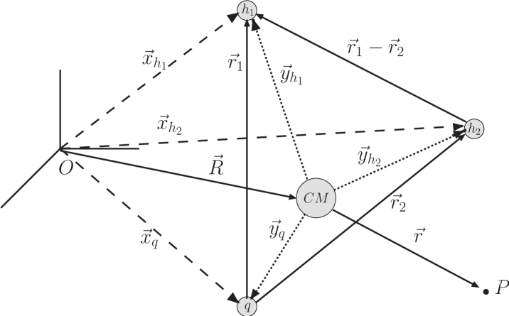
Figure 5.1: Definition of different coordinates used through this work.

In the Laboratory (LAB) frame (see Fig. 5.1), the Hamiltonian ($H$) of the three quark ($h_{1},\,h_{2},\,q$, where $h_{1},\,h_{2}=c,b$ and $q=l(u,\,d),\,s$) system reads:

$$H = \sum_{j=h_{1},\,h_{2},\,q}\left(m_{j}-\frac{\stackrel{{\scriptstyle\rightarrow}}{{\nabla}}\stackrel{{\scriptstyle}}{{{}^{2}}}_{\vec{x}_{j}}}{2m_{j}}\right)+V_{h_{1}h_{2}}+V_{h_{1}q}+V_{h_{2}q}$$ (5.1)

where $m_{h_{1}},\,m_{h_{2}},\,m_{q}$ are the quark masses and the quark-quark interaction terms $V_{jk}$ depend on the quark spin-flavor quantum numbers and the quark coordinates ($\vec{x}_{h_{1}},\vec{x}_{h_{2}},\,\vec{x}_{q}$ for the $h_{1},\,h_{2},\,q$ quarks respectively). To separate the Center of Mass (CM) free motion, we go to the light quark frame ($\vec{R},\vec{r}_{1},\vec{r}_{2}$),

$$\vec{R} = \frac{m_{h_{1}}\vec{x}_{h_{1}}+m_{h_{2}}\vec{x}_{h_{2}}+m_{q}\vec{x}_{q}}{m_{h_{1}}+m_{h_{2}}+m_{q}}$$

$$\vec{r}_{1} = \vec{x}_{h_{1}}-\vec{x}_{q}$$

$$\vec{r}_{2} = \vec{x}_{h_{2}}-\vec{x}_{q}$$ (5.2)

where $\vec{R}$ and $\vec{r}_{1},\,\vec{r}_{2}$ are the CM position in the LAB frame and the relative positions of the $h_{1},\,h_{2}$ heavy quarks with respect to the light quark $q$. The Hamiltonian now reads

$$H = -\frac{\stackrel{{\scriptstyle\rightarrow}}{{\nabla}}\stackrel{{\scriptstyle}}{{{}^{2}}}_{\vec{R}}}{2\overline{M}}+H^{\rm int}$$ (5.3)

$$H^{\rm int} = \sum_{j=1,2}\,H_{j}^{sp}+V_{h_{1}h_{2}}(\vec{r}_{1}-\vec{r}_{2},\,spin)-\frac{\stackrel{{\scriptstyle\rightarrow}}{{\nabla}}_{1}\cdot\stackrel{{\scriptstyle\rightarrow}}{{\nabla}}_{2}}{m_{q}}+\overline{M}$$

$$H_{j}^{sp} = -\frac{\stackrel{{\scriptstyle\rightarrow}}{{\nabla}}\stackrel{{\scriptstyle}}{{{}^{2}}}_{j}}{2\mu_{j}}+V_{h_{j}q}(\vec{r}_{j},\,spin),\ j=1,2$$ (5.4)

where $\overline{M}=m_{h_{1}}+m_{h_{2}}+m_{q}$, $\mu_{j}=\left(1/m_{h_{j}}+1/m_{q}\right)^{-1}$ and $\stackrel{{\scriptstyle\rightarrow}}{{\nabla}}_{j}=\partial/\partial_{\vec{r}_{j}},\ j=1,2$. The intrinsic Hamiltonian $H^{\rm int}$ describes the dynamics of the baryon. Apart from the sum of the quark masses $\overline{M}$, it consists of the sum of two single particle Hamiltonian $H^{sp}_{j}$, each of them describing the dynamics of a heavy-light quark system, plus the heavy–heavy interaction term, including the Hughes-Eckart term ($\stackrel{{\scriptstyle\rightarrow}}{{\nabla}}_{1}\cdot\stackrel{{\scriptstyle\rightarrow}}{{\nabla}}_{2}$). We will use a variational approach to solve it.

5.3 Variational Wave Functions

For the interactions presented in chapter 2, we have that both the total spin and the internal orbital angular momentum given as

$${\vec{S}} = \left({\vec{\sigma}}_{h_{1}}+{\vec{\sigma}}_{h_{2}}+{\vec{\sigma}}_{q}\right)/2$$

$${\vec{L}} = {\vec{l}}_{1}+{\vec{l}}_{2},\qquad{\rm with}~{}~{}{\vec{l}}_{j}=-{\rm i}~{}~{}{\vec{r}}_{j}\times{\stackrel{{\scriptstyle\rightarrow}}{{\nabla}}}_{j},\quad j=1,2$$ (5.5)

commute with the intrinsic Hamiltonian and are thus well defined. We are interested in the ground state of baryons with total angular momentum $J=1/2,\,3/2$ so that we can assume the orbital angular momentum of the baryons to be $L=0$. This implies that the spatial wave function can only depend on the relative distances $r_{1}$, $r_{2}$ and $r_{12}=|\vec{r}_{1}-\vec{r}_{2}|$. Furthermore when the heavy quark mass is infinity ($m_{h}\to\infty$), the total spin of the heavy degrees of freedom, $\vec{S}_{\rm heavy}=\left({\vec{\sigma}}_{h_{1}}+{\vec{\sigma}}_{h_{2}}\right)/2$, commutes with the intrinsic Hamiltonian, since the spin–spin terms in the potentials vanish in this limit. We can then assume the spin of the heavy degrees of freedom to be well defined.

With these simplifications we have used the following intrinsic wave functions in our variational approach

• $\Xi_{h_{1}h_{2}},\,\Omega_{h_{1}h_{2}}-$type baryons:

  $${|\Xi_{h_{1}h_{2}},\,\Omega_{h_{1}h_{2}};J=\frac{1}{2},M_{J}\rangle\,=}$$

  $$\sum_{M_{S_{h}}M_{S_{q}}}\left(\left.1,\frac{1}{2},\frac{1}{2}\right|M_{S_{h},}M_{S_{q},}M_{J}\right)\ |h_{1}h_{2};1M_{S_{h}}\rangle\otimes|q;\frac{1}{2}M_{S_{q}}\rangle\Psi_{h_{1}h_{2}}^{\Xi,\,\Omega}(r_{1},r_{2},r_{12})$$

  where $M_{J}$ is the third component of the baryon total angular momentum while $|h_{1}h_{2};S_{h},M_{S_{h}}\rangle$ and $|q;\frac{1}{2}M_{S_{q}}\rangle$ represent spin states of the $h_{1}h_{2}$ subsystem and the light quark respectively. For $h_{1}=h_{2}$ we need $\Psi_{h_{1}h_{1}}^{\Xi,\,\Omega}(r_{1},r_{2},r_{12})=\Psi_{h_{1}h_{1}}^{\Xi,\,\Omega}(r_{2},r_{1},r_{12})$ to guarantee a complete symmetry of the wave function under the exchange of the two heavy quarks.

• $\Xi^{*}_{h_{1}h_{2}},\,\Omega^{*}_{h_{1}h_{2}}-$type baryons:

  $$|\Xi^{*}_{h_{1}h_{2}},\,\Omega^{*}_{h_{1}h_{2}};J=\frac{3}{2},M_{J}\rangle\,=$$

  $$\sum_{M_{S_{h}}M_{S_{q}}}\left(\left.1,\frac{1}{2},\frac{3}{2}\right|M_{S_{h}},M_{S_{q}},M_{J}\right)\ |h_{1}h_{2};1M_{S_{h}}\rangle\otimes|q;\frac{1}{2}M_{S_{q}}\rangle\Psi_{h_{1}h_{2}}^{\Xi^{*},\,\Omega^{*}}(r_{1},r_{2},r_{12})$$

  Similarly to the case before for $h_{1}=h_{2}$ we need $\Psi_{h_{1}h_{1}}^{\Xi^{*},\,\Omega^{*}}(r_{1},r_{2},r_{12})=\Psi_{h_{1}h_{1}}^{\Xi^{*},\,\Omega^{*}}(r_{2},r_{1},r_{12})$.

• $\Xi^{\prime}_{h_{1}h_{2}},\,\Omega^{\prime}_{h_{1}h_{2}}-$type baryons:

  $$|\Xi^{\prime}_{h_{1}h_{2}},\,\Omega^{\prime}_{h_{1}h_{2}};J=\frac{1}{2},M_{J}\rangle = |h_{1}h_{2};00\rangle\otimes|q;\frac{1}{2}M_{J}\rangle\Psi_{h_{1}h_{2}}^{\Xi^{\prime},\,\Omega^{\prime}}(r_{1},r_{2},r_{12})$$ (5.8)

  In this case $h_{1}\neq h_{2}$ and we do not need the orbital part to have a definite symmetry under the exchange of the two quarks.

The spatial wave functions $\Psi(r_{1},r_{2},r_{12})$ in the above expressions will be determined by the variational principle: $\delta\langle B|H^{\rm int}|B\rangle=0$. For simplicity, we shall assume a Jastrow–type functional form:

$$\Psi_{h_{1}h_{2}}^{B}(r_{1},r_{2},r_{12}) = N\,F^{B}(r_{12})\,\phi_{h_{1}q}(r_{1})\,\phi_{h_{2}q}(r_{2})$$ (5.9)

where $N$ is a constant, which is determined from normalization

$$1 = \int d^{3}r_{1}\int d^{3}r_{2}\ \left|\Psi_{h_{1}h_{2}}^{B}(r_{1},r_{2},r_{12})\right|^{2}$$ (5.10)

$$= 8\pi^{2}\int_{0}^{+\infty}dr_{1}~{}r_{1}^{2}~{}\int_{0}^{+\infty}dr_{2}~{}r_{2}^{2}\int_{-1}^{+1}d\mu~{}\left|\Psi_{h_{1}h_{2}}^{B}(r_{1},r_{2},r_{12})\right|^{2}$$

with $\mu$ being the cosine of the angle between the vectors $\vec{r}_{1}$ and $\vec{r}_{2}$ ($r_{12}=(~{}r_{1}^{2}+r_{2}^{2}-2r_{1}r_{2}\mu)^{1/2}$).

The functions $\phi_{h_{1}q}$ and $\phi_{h_{2}q}$ will be taken as the $S-$wave ground states $\varphi_{j}(r_{j})$ of the single particle Hamiltonians $H^{sp}_{j}$ of Eq. (5.4) modified at large distances

$$\phi_{h_{j}q}(r_{j}) = (1+\alpha_{j}\,r_{j})\,\varphi_{j}(r_{j}),\ \ j=1,2$$ (5.11)

The heavy–heavy correlation function $F^{B}$ will be given by a linear combination of gaussians

$$F^{B}(r_{12}) = \sum_{j=1}^{4}a_{j}e^{-b_{j}^{2}(r_{12}+d_{j})^{2}},\quad a_{1}=1$$ (5.12)

The value of one of the $a_{j}$ parameters can be absorbed into the normalization constant $N$, so that we fix $a_{1}=1$. The values that we get for all parameters are given in appendix G.

5.3.1 Infinite heavy quark mass limit of variational wave functions

In the infinite heavy quark mass limit the wave function of the system should look like the one for a “meson” composed of a light quark and a heavy diquark. The two heavy quarks bind into a $\bar{3}$ color source diquark that to the light degrees of freedom appears to be pointlike [193]. In our model the pointlike nature of the heavy diquark comes about through the one-gluon exchange Coulomb potential which binds the two heavy quarks into a distance

$$r_{h_{1}h_{2}}\propto\frac{1}{\mu_{h_{1}h_{2}}};\ \mu_{h_{1}h_{2}}=\frac{m_{h_{1}}m_{h_{2}}}{m_{h_{1}}+m_{h_{2}}}$$ (5.13)

that tends to zero if both quark masses go to infinity.

For our wave functions we can define the probability distribution $P_{h1h2}$ for the two heavy quarks to be found at a distance $r_{h_{1}h_{2}}$

$$P_{h_{1}h_{2}}\,(r_{h_{1}h_{2}})=\int d^{3}r_{1}\int d^{3}r_{2}\ \delta(r_{12}-r_{h_{1}h_{2}})\left|\Psi^{B}_{h_{1}h_{2}}(r_{2},r_{2},r_{12})\right|^{2}$$ (5.14)

In Fig. 5.2, we show the $P_{h_{1}h_{2}}$ probability distributions for the $\Xi_{cc},\,\Xi_{bc},\,\Xi_{bb}$ and $\Omega_{cc},\,\Omega_{bc},\,\Omega_{bb}$ baryons evaluated for the AL1 potential.

Figure 5.2: $P_{h_{1}h_{2}}$ probabilities (see Eq.(5.14)) for the $\Xi_{cc},\,\Xi_{bc},\,\Xi_{bb}$ and $\Omega_{cc},\,\Omega_{bc},\,\Omega_{bb}$ baryons evaluated with the AL1 potential.

We see how the maximum moves, as expected, to lower $r_{h_{1}h_{2}}$ values as the quark masses increase.

On the other hand the relative wave function for the light quark with respect to the heavy quark subsystem should tend to the one of a light quark relative to a pointlike diquark. This limit is not evident in the coordinates we work as one has first to separate the diquark internal orbital wave function from the total one. To see that this limiting situation is in fact reached within our variational ansatz let us introduce the new set of coordinates

$$\vec{R} = \frac{m_{h_{1}}\vec{x}_{h_{1}}+m_{h_{2}}\vec{x}_{h_{2}}+m_{q}\vec{x}_{q}}{m_{h_{1}}+m_{h_{2}}+m_{q}}$$

$$\vec{r}_{12} = \vec{x}_{h_{1}}-\vec{x}_{h_{2}}$$

$$\vec{r}_{q} = \frac{m_{h_{1}}\vec{x}_{h_{1}}+m_{h_{2}}\vec{x}_{h_{2}}}{m_{h_{1}}+m_{h_{2}}}-\vec{x}_{q}=\frac{m_{h_{1}}\vec{r}_{1}+m_{h_{2}}\vec{r}_{2}}{m_{h_{1}}+m_{h_{2}}}$$ (5.15)

in terms of which the Hamiltonian now reads

$$H = -\frac{\stackrel{{\scriptstyle\rightarrow}}{{\nabla}}\stackrel{{\scriptstyle}}{{{}^{2}}}_{\vec{R}}}{2\overline{M}}+H^{\rm int}$$

$$H^{\rm int} = \overline{M}+H_{h_{1}h_{2}}+H_{qh_{1}h_{2}}$$ (5.16)

where

$$H_{h1h_{2}} = -\frac{\stackrel{{\scriptstyle\rightarrow}}{{\nabla}}_{12}^{2}}{2\mu_{h_{1}h_{2}}}+V_{h_{1}h_{2}}(\vec{r}_{12},\,spin)$$

$$H_{qh_{1}h_{2}} = -\frac{1}{2}\left(\frac{1}{m_{h_{1}}+m_{h_{2}}}+\frac{1}{m_{q}}\right)\stackrel{{\scriptstyle\rightarrow}}{{\nabla}}_{q}^{2}+V_{h_{1}q}(\vec{r}_{q}+\frac{m_{h_{2}}}{m_{h_{1}}+m_{h_{2}}}\vec{r}_{12},\,spin)$$ (5.17)

$$\hskip 129.46011pt+V_{h_{2}q}(\vec{r}_{q}-\frac{m_{h_{1}}}{m_{h_{1}}+m_{h_{2}}}\vec{r}_{12},\,spin)$$

with $\stackrel{{\scriptstyle\rightarrow}}{{\nabla}}_{12}=\partial/\partial_{\vec{r}_{12}}$ and $\stackrel{{\scriptstyle\rightarrow}}{{\nabla}}_{q}=\partial/\partial_{\vec{r}_{q}}$. Defining now

$$H^{0}_{qh_{1}h_{2}} = -\frac{1}{2}\left(\frac{1}{m_{h_{1}}+m_{h_{2}}}+\frac{1}{m_{q}}\right)\stackrel{{\scriptstyle\rightarrow}}{{\nabla}}_{q}^{2}+V_{h_{1}q}(\vec{r}_{q},\,spin)+V_{h_{2}q}(\vec{r}_{q},\,spin)$$ (5.18)

one would have

$$H^{\mathrm{int}}=H_{h_{1}h_{2}}+H^{0}_{qh_{1}h_{2}}+(H_{qh_{1}h_{2}}-H^{0}_{qh_{1}h_{2}})$$ (5.19)

$H_{h_{1}h_{2}}$ is the Hamiltonian for the relative movement of the two heavy quarks while $H^{0}_{qh_{1}h_{2}}$ is the Hamiltonian for the relative movement of the light quark with respect to a pointlike heavy diquark where the two heavy quarks are located in their center of mass. Both movements are coupled through the term $(H_{qh_{1}h_{2}}-H^{0}_{qh_{1}h_{2}})$. If the heavy quark masses get arbitrarily large the average $r_{12}$ value tends to zero and thus one can neglect the effect of $H_{qh_{1}h_{2}}-H^{0}_{qh_{1}h_{2}}$. In that limiting situation the light and heavy quark degrees of freedom decouple completely and the internal Hamiltonian reduces, as it should, to the sum of the Hamiltonians $H_{h_{1}h_{2}}$, corresponding to the relative movement of the two heavy quarks, and $H^{0}_{qh_{1}h_{2}}$, corresponding to the relative movement of the light quark with respect to the pointlike heavy diquark subsystem.

As to the wave function it should reduce in that limit to the product $\Phi_{h_{1}h_{2}}(r_{12})\cdot\Phi^{0}_{qh_{1}h_{2}}(r_{q})$, being $\Phi_{h_{1}h_{2}}(r_{12}),\,\Phi^{0}_{qh_{1}h_{2}}(r_{q})$ the ground state wave functions for $H_{h_{1}h_{2}},$ $H^{0}_{qh_{1}h_{2}}$ respectively. To check that we reach that limiting situation we have evaluated the projection ${\cal P}$ of our variational wave functions onto $\Phi_{h_{1}h_{2}}(r_{12})\cdot\Phi^{0}_{qh_{1}h_{2}}(r_{q})$ evaluated with the actual heavy quark masses. This projection is given by

$${\cal P}=\int d^{3}r_{1}\int d^{3}r_{2}\left(\Psi^{B}_{h_{1}h_{2}}(r_{1},r_{2},r_{12}\right)^{*}\Phi_{h_{1}h_{2}}(r_{12})\ \Phi^{0}_{qh_{1}h_{2}}(r_{q})$$ (5.20)

and the values for $|{\cal P}|^{2}$ that we obtain for the $\Xi_{cc},\,\Xi_{bc},\,\Xi_{bb}$ and $\Omega_{cc},\,\Omega_{bc},\,\Omega_{bb}$ baryons using the AL1 potential are given in Table 5.2. We see how $|{\cal P}|^{2}$ increases with increasing heavy quark masses indicating that for very high heavy quark masses the total wave function tends to the one of a light quark relative to a pointlike diquark times the diquark internal wave function.

	$\Xi_{cc}$	$\Xi_{bc}$	$\Xi_{bb}$	$\Omega_{cc}$	$\Omega_{bc}$	$\Omega_{bb}$
$|{\cal P}|^{2}$	0.974	0.975	0.991	0.959	0.966	0.984

Table 5.2: Absolute value square of the ${\cal P}$ projection coefficient defined in Eq. (5.20)

In summary, our variational wave functions respect the infinite heavy quark mass limit.

We note by passing that the product $\Phi_{h_{1}h_{2}}(r_{12})\cdot\Phi^{0}_{qh_{1}h_{2}}(r_{q})$ corrected by a correlation function in the variable $\vec{r}_{12}\cdot\vec{r}_{q}$ would have been a good variational orbital wave function. For instance, a calculation using the AL1 potential and an orbital wave function given just by that product $\Phi_{h_{1}h_{2}}(r_{12})\cdot\Phi^{0}_{qh_{1}h_{2}}(r_{q})$ gives for the expectation value of $H^{\mathrm{int}}$ for the $\Xi_{cc},\,\Xi_{bc},\,\Xi_{bb}$ baryons

$$\left.\langle H^{\mathrm{int}}\rangle\right|^{AL1}_{\Xi_{cc}}=3640\,\mathrm{MeV};\ \left.\langle H^{\mathrm{int}}\rangle\right|^{AL1}_{\Xi_{bc}}=6943\,\mathrm{MeV};\ \left.\langle H^{\mathrm{int}}\rangle\right|^{AL1}_{\Xi_{bb}}=10198\,\mathrm{MeV}$$ (5.21)

which are respectively 28 MeV, 24 MeV, and 1 MeV larger, and therefore worse, than our best values in Table 5.3. The correlation function would clearly be needed, being its role more important for the “$cc$” and “$bc$” systems. The improvement in going from a “$cc$” to a “$bc$ system” is not as good as one would naively expect, the reason being that, considering $\vec{r}_{12}$ to be a small quantity, $H_{qh_{1}h_{2}}-H^{0}_{qh_{1}h_{2}}$ is first order in $\vec{r}_{12}$ for the “$bc$” system while, for symmetry reasons, it is necessarily of second order for the “$cc$” and “$bb$” ones. In any case one sees how the expectation values obtained with this simple ansatz get closer to our best values in Table 5.3 as the heavy quark masses increase.

5.4 Static Properties

5.4.1 Masses

The mass of the baryon is simply given by the expectation value of the intrinsic Hamiltonian. Our results (VAR) appear in Table 5.3 where we compare them with the ones obtained in Ref. [75] with the use of the same inter-quark interactions but within a Faddeev approach (FAD). For that purpose we have eliminated from the latter a small three-body force contribution of the type $V_{123}={\rm constant}/m_{h_{1}}m_{h_{2}}m_{q}$ that was also included in the evaluation of Ref. [75]. We will show their full results in the following tables. Whenever comparison is possible we find an excellent agreement between the two calculations. In some cases the variational masses are even lower than the Faddeev ones. Besides we give predictions for states that were not considered in the study of Ref. [75].

		AL1	AL2	AP1	AP2	BHAD
$\Xi_{cc}$	VAR	3612	3619	3629	3630	3639
	FAD [75]	3609	3616	3625	3628	3633
$\Xi_{cc}^{*}$	VAR	3706	3715	3722	3729	3722
$\Xi_{bb}$	VAR	10197	10180	10207	10179	10202
	FAD [75]	10194	10175	10204	10176	10197
$\Xi_{bb}^{*}$	VAR	10236	10219	10245	10219	10235
$\Xi_{bc}$	VAR	6919	6912	6933	6917	6936
	FAD [75]	6916	6913	6928	6907	6934
$\Xi_{bc}^{\prime}$	VAR	6948	6942	6957	6944	6965
$\Xi_{bc}^{*}$	VAR	6986	6981	7000	6987	6993

		AL1	AL2	AP1	AP2	BHAD
$\Omega_{cc}$	VAR	3702	3718	3711	3710	3743
	FAD [75]	3711	3718	3710	3709	3741
$\Omega_{cc}^{*}$	VAR	3783	3802	3800	3802	3805
$\Omega_{bb}$	VAR	10260	10249	10259	10226	10274
	FAD [75]	10267	10246	10258	10224	10271
$\Omega_{bb}^{*}$	VAR	10297	10287	10301	10269	10302
$\Omega_{bc}$	VAR	6986	6986	6990	6969	7013
	FAD [75]	7003	6996	6996	6971	7023
$\Omega_{bc}^{\prime}$	VAR	7009	7010	7011	6994	7033
$\Omega_{bc}^{*}$	VAR	7046	7047	7055	7037	7057

Table 5.3: Doubly heavy $\Xi$ and $\Omega$ baryons masses in MeV. VAR stands for the results of our variational calculation. FAD stands for the results obtained in Ref. [75] using the same interquark interactions but within a Faddeev approach.

In Tables 5.4 and 5.5 we compare our results with other theoretical calculations. Our central values correspond to the results obtained with the AL1 potential, while the errors quoted take into account the variation when using different potentials. The same presentation is used for the results obtained in Ref. [75] for which we now show their full values including the contribution of the three-body force. All calculations give similar results that vary within a few per cent. From the experimental point of view the SELEX Collaboration [195] has recently measured the value of $m_{\Xi_{cc}}$. This experimental value is 100 MeV smaller that our result. On account of what has been said in the introduction to this chapter , one should take this experimental value with due caution. Note also that in Ref. [195] the systematic error is not given. There are also different lattice determinations for baryons with two equal heavy quarks [212, 213, 214]. Our results agree within errors with the lattice data for baryons with two $c$ quarks, while they are roughly 100 MeV below lattice results for doubly $b$-quark baryons. The best overall agreement with lattice data available so far is achieved in the calculation of Ref. [209, 210] where they use the Feynman-Hellmann theorem and semiempirical mass formulas in the framework of a nonrelativistic quark model but without the use of an explicit Hamiltonian. Within full dynamical calculations, ours and the relativistic calculations in Refs. [201, 204, 208] have the best overall agreement with lattice data.

	This work	[75]	[201]	[202]	[203]	[204]	[205]	[206]	[207]	[208]	[209, 210]	[65]	[211]
$\Xi_{cc}$	$3612^{+17}$	$3607^{+24}$	3620	3480	3690	3740	3646	3524	3478	3660	$3660\pm 70$	3610	$3588\pm 72$
$\Xi^{*}_{cc}$	$3706^{+23}$		3727	3610		3860	3733	3548	3610	3810	$3740\pm 80$	3680
$\Xi_{bb}$	$10197^{+10}_{-17}$	$10194^{+10}_{-19}$	10202	10090	10160	10300			10093	10230	$10340\pm 100$
$\Xi^{*}_{bb}$	$10236^{+9}_{-17}$		10237	10130		10340			10133	10280	$10370\pm 100$
$\Xi_{bc}$	$6919^{+17}_{-7}$	$6915^{+17}_{-9}$	6933	6820	6960	7010			6820	6950	$6965\pm 90$†		$6840\pm 236$
$\Xi^{\prime}_{bc}$	$6948^{+17}_{-6}$		6963	6850		7070			6850	7000	$7065\pm 90$†
$\Xi^{*}_{bc}$	$6986^{+14}_{-5}$		6980	6900		7100			6900	7020	$7060\pm 90$

	This work	Exp. [195]	Latt. [212]	Latt. [213]	Latt. [214]
$\Xi_{cc}$	$3612^{+17}$	$3519\pm 1$		$3605\pm 23$	$3549\pm 95$
$\Xi^{*}_{cc}$	$3706^{+23}$			$3685\pm 23$	$3641\pm 97$
$\Xi_{bb}$	$10197^{+10}_{-17}$		$10314\pm 47$
$\Xi^{*}_{bb}$	$10236^{+9}_{-17}$		$10333\pm 55$

Table 5.4: First panel: doubly heavy $\Xi$ masses in MeV as obtained in different models. Our central values, and the ones of Ref. [75], have been evaluated with the AL1 potential. Second panel: we compare our results with the experimental value for $M_{\Xi_{cc}}$ measured by the SELEX Collaboration [195] (Note the cautions that appear on this experimental mass in the introduction to this chapter), and lattice results from Refs. [212, 213, 214]. Entries with ^† should be taken with due caution (see text).

	This work	[75]	[201]	[202]	[203]	[204]	[205]	[207]	[208]	[209, 210]	[65]	[211]
$\Omega_{cc}$	$3702^{+41}$	$3710^{+29}_{-2}$	3778	3590	3860	3760	3749	3590	3760	$3740\pm 70$	3710	$3698\pm 65$
$\Omega^{*}_{cc}$	$3783^{+22}$		3872	3690		3900	3826	3690	3890	$3820\pm 80$	3760
$\Omega_{bb}$	$10260^{+14}_{-34}$	$10267^{+4}_{-43}$	10359	10180	10340	10340		10180	10320	$10370\pm 100$
$\Omega^{*}_{bb}$	$10297^{+5}_{-28}$		10389	10200		10380		10200	10360	$10400\pm 100$
$\Omega_{bc}$	$6986^{+27}_{-17}$	$7003^{+20}_{-32}$	7088	6910	7130	7050		6910	7050	$7045\pm 90$†		$6954\pm 225$
$\Omega^{\prime}_{bc}$	$7009^{+24}_{-15}$		7116	6930		7110		6930	7090	$7105\pm 90$†
$\Omega^{*}_{bc}$	$7046^{+11}_{-9}$		7130	6990		7130		6990	7110	$7120\pm 90$

	This work	Latt. [212]	Latt. [213]	Latt. [214]
$\Omega_{cc}$	$3702^{+41}$		$3733\pm 9^{+7}_{-38}$	$3663\pm 97$
$\Omega^{*}_{cc}$	$3783^{+22}$		$3801\pm 9^{+3}_{-34}$	$3734\pm 98$
$\Omega_{bb}$	$10260^{+14}_{-34}$	$10365\pm 40^{-11}_{+12}$${}^{+16}_{-0}$
$\Omega^{*}_{bb}$	$10297^{+5}_{-28}$	$10383\pm 39^{-8}_{+8}$${}^{+12}_{-0}$

Table 5.5: Same as Table 5.4 for doubly heavy $\Omega$ baryons.

There are also independent determinations of mass splittings in lattice QCD [212, 213, 214], nonrelativisitic lattice QCD [211] and pNRQCD [194]. In Table 5.6 we compare those results to the ones obtained in the present calculation and in other models.

	This work	[201]	[202]	[204]	[207]	[208]	[194]	[211]	Latt. [212]	Latt. [213]	Latt. [214]
$M_{\Xi^{*}_{cc}}-M_{\Xi_{cc}}$	$94^{+5}_{-11}$	107	130	120	132	150	$120\pm 40$	$70\pm 13$		$80\pm 11$	$87\pm 19$
$M_{\Xi^{*}_{bb}}-M_{\Xi_{bb}}$	$39^{+1}_{-6}$	35	40	40	40	50	$34\pm 4$	$20\pm 7$	$20\pm 6$
$M_{\Xi^{*}_{bc}}-M_{\Xi_{B^{\prime}s}}$	$67^{+3}_{-10}$	47	80	90	80	70		$43\pm 11$
$M_{\Xi^{\prime}_{bc}}-M_{\Xi_{bc}}$	$29^{+1}_{-5}$	30	30	60	30	50		$9\pm 7$
$M_{\Omega^{*}_{cc}}-M_{\Omega_{cc}}$	$81^{+11}_{-19}$	94	100	140	100	130		$63\pm 9$		$68\pm 7$	$67\pm 16$
$M_{\Omega^{*}_{bb}}-M_{\Omega_{bb}}$	$37^{+6}_{-9}$	30	20	40	20	40		$19\pm 5$	$20\pm 5$
$M_{\Omega^{*}_{bc}}-M_{\Omega_{bc}}$	$60^{+8}_{-16}$	42	80	80	80	60		$39\pm 8$
$M_{\Omega^{\prime}_{bc}}-M_{\Omega_{bc}}$	$23^{+2}_{-3}$	28	20	60	20	40		$9\pm 6$

Table 5.6: Mass splittings in MeV for doubly heavy $\Xi$ and $\Omega$ baryons. Our central values have been obtained with the AL1 potential.

Our central results evaluated with the AL1 potential are larger than the ones obtained in lattice QCD [212, 213, 214] and lattice nonrelativistic QCD [211]. The agreement is better when we use the BHAD potential of Ref. [73] for which we get the lowest results. Similar results are obtained by the relativistic calculation of Ref. [201], whereas for the relativistic calculations in Refs. [202, 204, 208] and the nonrelativistic one in Ref. [207] the agreement with lattice QCD and nonrelativistic lattice QCD data worsens. As for the calculations in Ref. [209, 210] we do not quote their results due to the large theoretical errors involved.

5.4.2 Charge densities and radii

The baryon charge density at the point $P$ (coordinate vector $\vec{r}$ in the CM frame, see Fig. 5.1) is given by:

$$\rho_{e}^{B}(\vec{r}\,) = \int d^{3}r_{1}d^{3}r_{2}\ \Big{|}\Psi_{h_{1}h_{2}}^{B}(r_{1},r_{2},r_{12})\Big{|}^{2}$$ (5.23)

$$\hskip 28.45274pt\left\{e_{h_{1}}\delta^{3}(\vec{r}-\vec{y}_{h_{1}})+e_{h_{2}}\delta^{3}(\vec{r}-\vec{y}_{h_{2}})+e_{q}\delta^{3}(\vec{r}-\vec{y}_{q})\right\}$$

$$\equiv \rho_{e}^{B}(\vec{r}\,)\big{|}_{h_{1}}+\rho_{e}^{B}(\vec{r}\,)\big{|}_{h_{2}}+\rho_{e}^{B}(\vec{r}\,)\big{|}_{q}$$

where $e_{h_{1},\,h_{2},\,q}$ are the quark charges in proton charge units $e$, and from Fig. 5.1 we have $\vec{y}_{h_{1}}=\vec{y}_{q}+\vec{r}_{1}$, $\vec{y}_{h_{2}}=\vec{y}_{q}+\vec{r}_{2}$ and $\vec{y}_{q}=-\left(m_{h_{1}}\vec{r}_{1}+m_{h_{2}}\vec{r}_{2}\right)/\overline{M}$. Since our $L=0$ wave functions only depend on scalars ($r_{1},r_{2}$ and $r_{12}$) the charge density is spherically symmetric ($\rho_{e}^{B}(\vec{r}\,)=\rho_{e}^{B}(|\vec{r}~{}|)$).

The charge form factor is defined as usual

$${\cal F}_{e}^{B}(\vec{q}~{})=\int d^{3}r\ e^{{\rm i}\vec{q}\cdot\vec{r}}\rho_{e}^{B}(r)$$ (5.24)

and it only depends on $|\vec{q}~{}|$. Its value at $\vec{q}=\vec{0}$ gives the baryon charge in units of the proton charge.

The charge mean square radii are defined

$$\langle r^{2}\rangle_{e}^{B}=\int d^{3}r\ r^{2}\rho_{e}^{B}(r)=4\pi\int_{0}^{+\infty}dr\ r^{4}\rho_{e}^{B}(r)$$ (5.25)

Figure 5.3: Charge form factor of the $\Xi_{cc},\,\Xi_{bb}$ and $\Xi^{*}_{cc},\,\Xi^{*}_{bb}$ baryons evaluated with the AL1 (solid line) and BHAD (dashed line) potentials. We show the two possible charge states.

Figure 5.4: Charge form factor of the $\Omega_{cc},\,\Omega_{bb}$ and $\Omega^{*}_{cc},\,\Omega^{*}_{bb}$ baryons evaluated with the AL1 (solid line) and BHAD (dashed line) potentials.

In Figs. 5.3, 5.4 and 5.5 we show the charge form factors for the different doubly heavy baryons under study including the two different charge states for the doubly heavy $\Xi$ ones. We show the calculations with both the AL1 potential and the BHAD potential. The differences between the two calculations are minor in most cases.

Figure 5.5: Charge form factor of the $\Xi_{bc},\,\Xi^{*}_{bc},\,\Xi^{\prime}_{bc}$ and $\Omega_{bc},\,\Omega^{*}_{bc}\,\Omega^{\prime}_{bc}$ baryons evaluated with the AL1 (solid line) and BHAD (dashed line) potentials. For the $\Xi$ baryons we show the two possible charge states.

In Table 5.7 we show the charge mean square radii. With the exceptions of the $\Xi_{bc}^{0}$ and $\Omega_{bc}^{0}$, we find good agreement with the results obtained in Ref. [75] within a Faddeev calculation. The possible presence of a $S_{h}=0$ contribution in the wave functions of Ref. [75] could be the possible explanation for this discrepancy. We also compare with the results obtained, for a few states, in Ref. [216] with the use a relativistic quark model in the instant form. The agreement is bad in this case.

	This work	[75]	[216]
$\Xi_{cc}^{+}$	$-0.030^{+0.003}_{-0.016}$	$-0.038^{+0.004}_{-0.016}$	$0.1$
$\Xi_{cc}^{++}$	$0.298^{+0.034}_{-0.028}$	$0.315^{+0.035}_{-0.030}$	$1.3$
$\Xi_{cc}^{*+}$	$-0.042^{+0.007}_{-0.019}$
$\Xi_{cc}^{*++}$	$0.341^{+0.041}_{-0.042}$
$\Xi_{bb}^{0}$	$0.221^{+0.033}_{-0.025}$	$0.242^{+0.035}_{-0.027}$
$\Xi_{bb}^{-}$	$-0.133^{+0.014}_{-0.016}$	$-0.143^{+0.006}_{-0.018}$
$\Xi_{bb}^{*-}$	$-0.142^{+0.018}_{-0.018}$
$\Xi_{bb}^{*0}$	$0.238^{+0.035}_{-0.031}$
$\Xi_{bc}^{0}$	$-0.057^{+0.006}_{-0.013}$	$-0.072^{+0.008}_{-0.017}$
$\Xi_{bc}^{+}$	$0.279^{+0.026}_{-0.031}$	$0.306^{+0.035}_{-0.011}$
$\Xi_{bc}^{\prime 0}$	$-0.065^{+0.010}_{-0.015}$
$\Xi_{bc}^{\prime+}$	$0.283^{+0.036}_{-0.025}$
$\Xi_{bc}^{*0}$	$-0.065^{+0.010}_{-0.018}$
$\Xi_{bc}^{*+}$	$0.305^{+0.031}_{-0.039}$

	This work	[75]	[216]
$\Omega_{cc}^{+}$	$0.013^{+0.001}_{-0.002}$	$0.009_{-0.003}$	$0.2$
$\Omega_{cc}^{*+}$	$0.009^{+0.001}_{-0.002}$
$\Omega_{bb}^{-}$	$-0.086^{+0.008}_{-0.001}$	$-0.090^{+0.007}_{-0.002}$
$\Omega_{bb}^{*-}$	$-0.092^{+0.011}_{-0.001}$
$\Omega_{bc}^{0}$	$-0.016_{+0.003}$	$-0.025^{+0.002}_{-0.003}$
$\Omega_{bc}^{\prime 0}$	$-0.019^{+0.003}_{-0.003}$
$\Omega_{bc}^{*0}$	$-0.021^{+0.004}_{-0.002}$

Table 5.7: Charge mean square radii in fm² for doubly heavy $\Xi$ and $\Omega$ baryons. Our central values, and the ones of Ref. [75], have been evaluated with the AL1 potential.

5.4.3 Magnetic moments

The orbital part of the magnetic moment is defined in terms of the velocities $\vec{v}$ of the quarks, with respect to the position of the CM, and it reads

$${\mu}^{B} = \int d^{3}r_{1}d^{3}r_{2}\left(\Psi_{h_{1}h_{2}}^{B}(r_{1},r_{2},r_{12})\right)^{*}\left\{\frac{e_{h_{1}}}{2m_{h_{1}}}(\vec{y}_{h_{1}}\times m_{h_{1}}\vec{v}_{{h_{1}}})_{z}\right.$$ (5.26)

$$+ \left.\frac{e_{h_{2}}}{2m_{h_{2}}}(\vec{y}_{h_{2}}\times m_{h_{2}}\vec{v}_{h_{2}})_{z}+\frac{e_{q}}{2m_{q}}(\vec{y}_{q}\times m_{q}\vec{v}_{y_{q}})_{z}\right\}\Psi_{h_{1}h_{2}}^{B}(r_{1},r_{2},r_{12})$$

with $m_{h_{1}}\vec{v}_{h_{1}}=-i\vec{\nabla}_{1}$, $m_{h_{2}}\vec{v}_{h_{2}}=-i\vec{\nabla}_{2}$ and $m_{q}\vec{v}_{q}=i\left(\vec{\nabla}_{1}+\vec{\nabla}_{2}\right)$.

Since our orbital wave function has $L=0$, the orbital magnetic moment vanishes. The magnetic moment of the baryon is then entirely given by the spin contribution.

$$\langle B;\,J,\,M_{J}=J|\ \frac{e_{h_{1}}}{2m_{h_{1}}}(\vec{\sigma}_{h_{1}})_{z}+\frac{e_{h_{2}}}{2m_{h_{2}}}(\vec{\sigma}_{h_{2}})_{z}+\frac{e_{q}}{2m_{q}}(\vec{\sigma}_{q})_{z}\ |B;\,J,\,M_{J}=J\rangle$$ (5.28)

Those matrix elements are trivially evaluated with the results

$$\Xi_{h1h_{2}},\ \Omega_{h1h_{2}} \longrightarrow \frac{2}{3}\left(\frac{e_{h_{1}}}{2m_{h_{1}}}+\frac{e_{h_{2}}}{2m_{h_{2}}}-\frac{1}{2}\ \frac{e_{q}}{2m_{q}}\right)$$

$$\Xi^{*}_{h1h_{2}},\ \Omega^{*}_{h1h_{2}} \longrightarrow \frac{e_{h_{1}}}{2m_{h_{1}}}+\frac{e_{h_{2}}}{2m_{h_{2}}}+\frac{e_{q}}{2m_{q}}$$

$$\Xi^{\prime}_{h1h_{2}},\ \Omega^{\prime}_{h1h_{2}} \longrightarrow \frac{e_{q}}{2m_{q}}$$ (5.29)

In Table 5.8 we give our numerical results. Our central values, as the ones obtained in Ref. [75] within a Faddeev approach, have been evaluated with the use of the AL1 potential. When compared to the values obtained in Ref. [75] we find very good agreement with just a few exceptions ($\Xi_{bc}^{0},\,\Xi_{bc}^{+},\,\Omega_{bc}^{0}$). The discrepancy for the latter baryons may come from a possible non negligible $S_{h}=0$ contribution to their wave functions in the calculation of Ref. [75]. In our case we have fixed $S_{h}=1$ which we think is a very good approximation since in the limit of infinite heavy quark masses the spin of the heavy quark degrees of freedom is well defined.

We also compare our results to the ones obtained in Refs.[191, 215, 216, 217, 218, 219] using different approaches. The differences between different calculations are in some cases large. Being $L=0$ a good approximation the magnetic moments are essentially determined by the spin contribution of the quarks. With $m_{b}\gg m_{u},\,m_{d},\,m_{s}$, the contribution from the $b$ quarks is negligible compared to the one of the light quark. This is also true to a lesser extent for the $c$ quark.

	This work	[75]	[191]	[215]	[216]	[217]	[218]	[219]
$\Xi_{cc}^{+}$	$0.785^{+0.050}_{-0.030}$	$0.784^{+0.050}_{-0.029}$	0.806	0.72	$0.72$	$0.89\sim 0.98$	$0.778\sim 0.790$	0.86
$\Xi_{cc}^{++}$	$-0.208^{+0.035}_{-0.086}$	$-0.206^{+0.034}_{-0.086}$	$-0.124$	0.13	$-0.10$	$-0.47$	$-0.172\sim-0.154$	0.17
$\Xi_{cc}^{*+}$	$-0.311^{+0.052}_{-0.130}$		$-0.186$			$-1.17\sim-0.98$		0.20
$\Xi_{cc}^{*++}$	$2.67^{+0.27}_{-0.15}$		2.60			$3.16\sim 3.18$		2.54
$\Xi_{bb}^{0}$	$-0.742^{+0.044}_{-0.091}$	$-0.742^{+0.044}_{-0.092}$		$-0.53$			$-0.726\sim-0.705$	0.61
$\Xi_{bb}^{-}$	$0.251^{+0.045}_{-0.021}$	$0.251^{+0.046}_{-0.021}$		0.18			$0.226\sim 0.236$	0.14
$\Xi_{bb}^{*0}$	$1.87^{+0.27}_{-0.13}$							1.37
$\Xi_{bb}^{*-}$	$-1.11^{+0.06}_{-0.14}$							$-0.95$
$\Xi_{bc}^{0}$	$0.518^{+0.048}_{-0.020}$	$0.058^{+0.059}_{-0.054}$		0.42
$\Xi_{bc}^{+}$	$-0.475^{+0.040}_{-0.088}$	$-0.198^{+0.057}_{-0.056}$		$-0.12$
$\Xi_{bc}^{\prime 0}$	$-0.993^{+0.065}_{-0.137}$			$-0.76$			$-0.385\sim-0.366$
$\Xi_{bc}^{\prime+}$	$1.99^{+0.27}_{-0.13}$			1.52			$1.50\sim 1.54$
$\Xi_{bc}^{*0}$	$-0.712^{+0.059}_{-0.133}$							$-0.39$
$\Xi_{bc}^{*+}$	$2.27^{+0.27}_{-0.14}$							2.04

	This work	[75]	[191]	[215]	[216]	[217]	[218]	[219]
$\Omega_{cc}^{+}$	$0.635^{+0.012}_{-0.015}$	$0.635^{+0.011}_{-0.015}$	0.688	0.67	$0.72$	$0.59\sim 0.64$	$0.657\sim 0.663$	0.84
$\Omega_{cc}^{*+}$	$0.139^{+0.009}_{-0.017}$		0.167			$-0.20\sim 0.03$		0.39
$\Omega_{bb}^{-}$	$0.101^{+0.007}_{-0.007}$	$0.101^{+0.007}_{-0.006}$		0.04			$0.105\sim 0.108$	0.084
$\Omega_{bb}^{*-}$	$-0.662^{+0.022}_{-0.024}$							$-1.28$
$\Omega_{bc}^{0}$	$0.368^{+0.010}_{-0.011}$	$0.009^{+0.038}_{-0.029}$		0.45
$\Omega_{bc}^{\prime 0}$	$-0.542^{+0.021}_{-0.024}$			$-0.61$			$-0.130\sim-0.125$
$\Omega_{bc}^{*0}$	$-0.261^{+0.015}_{-0.021}$							$-0.22$

Table 5.8: Magnetic moments, in nuclear magnetons ($e/2m_{p}$, with $m_{p}$ the proton mass), of doubly heavy $\Xi$ and $\Omega$ baryons. Our central values, and the ones of Ref. [75], have been evaluated with the AL1 potential.

Chapter 6 Doubly heavy baryons semileptonic decay

6.1 Introduction

In this chapter we should use the manageable wave functions that we got in chapter 5 to study semileptonic decays of doubly, $J=1/2$, baryons. All the transitions studied here involve a $b\to c$ transition at the quark level. We shall evaluate form factors, decay widths and angular asymmetry parameters. Previous calculations of semileptonic decay widths have been done in different relativistic quark model approaches  [220, 221, 222], or with the use of HQET [179].

6.2 Decay width and angular asymmetries

The differential decay width for a $B(1/2^{+})\to B^{\prime}(1/2^{+})$ transition reads

$${\rm d}\Gamma=8|V_{cb}|^{2}m_{B^{\prime}}G_{F}^{\,2}\frac{d^{3}p^{\prime}}{(2\pi)^{3}2E^{\prime}_{B^{\prime}}(\vec{p}^{\prime})}\frac{d^{3}k}{(2\pi)^{3}2E_{\bar{\nu}_{l}}(\vec{k})}\frac{d^{3}k^{\prime}}{(2\pi)^{3}2E^{\prime}_{l}(\vec{k}^{\prime})}\$$

$$\hskip 85.35826pt\times(2\pi)^{4}\delta^{4}(p-p^{\prime}-k-k^{\prime}){\cal L}^{\alpha\beta}(k,k^{\prime}){\cal H}_{\alpha\beta}(p,p^{\prime})$$ (6.1)

where $|V_{cb}|$ is the modulus of the corresponding CKM matrix element, $m_{B^{\prime}}$ is the mass of the final baryon, $p$, $p^{\prime}$, $k$ and $k^{\prime}$ are the four-momenta of the initial baryon, final baryon, final anti-neutrino and final lepton respectively, and ${\cal L}$ and ${\cal H}$ are the lepton and hadron tensors.

The lepton tensor is given as

$${\cal L}^{\mu\sigma}(k,k^{\prime}) = k^{\prime\mu}k^{\sigma}+k^{\prime\sigma}k^{\mu}-g^{\mu\sigma}k\cdot k^{\prime}-{\rm i}\epsilon^{\mu\sigma\alpha\beta}k^{\prime}_{\alpha}k_{\beta}$$ (6.2)

As for the hadron tensor we have

$${\cal H}_{\mu\sigma}(p,p^{\prime}) = \frac{1}{2}\sum_{r,r^{\prime}}\left\langle B^{\prime},r^{\prime}\ \vec{p}^{\,\prime}\left|\,\overline{\Psi}^{c}(0)\gamma_{\mu}(I-\gamma_{5})\Psi^{b}(0)\right|B,r\ \vec{p}\right\rangle$$ (6.3)

$$\hskip 73.97733pt\left\langle B^{\prime},r^{\prime}\ \vec{p}^{\,\prime}\left|\,\overline{\Psi}^{c}(0)\gamma_{\sigma}(I-\gamma_{5})\Psi^{b}(0)\right|B,r\ \vec{p}\right\rangle^{*}$$

with $\left|B,r\ \vec{p}\right\rangle\,(\left|B^{\prime},r^{\prime}\ \vec{p}\,^{\prime}\right\rangle)$ representing the initial (final) baryon with three–momentum $\vec{p}$ ($\vec{p}\,^{\prime}$) and spin third component $r$ ($r^{\prime}$). The baryon states are here normalized such that $\langle r\ \vec{p}\,|\,r^{\prime}\ \vec{p}^{\,\prime}\rangle=(2\pi)^{3}(E(\vec{p}\,)/m)\,\delta_{rr^{\prime}}\,\delta^{3}(\vec{p}-\vec{p}^{\,\prime})$. The hadron matrix elements can be parametrized in terms of six form factors as

$$\left\langle B^{\prime},r^{\prime}\ \vec{p}^{\,\prime}\left|\,\overline{\Psi}^{c}(0)\gamma_{\mu}(I-\gamma_{5})\Psi^{b}(0)\right|B,r\ \vec{p}\right\rangle\,=$$ (6.4)

$$=\,{\bar{u}}^{B^{\prime}}_{r^{\prime}}(\vec{p}^{\,\prime})\Big{\{}\gamma_{\mu}\left(F_{1}(w)-\gamma_{5}G_{1}(w)\right)+v_{\mu}\left(F_{2}(w)-\gamma_{5}G_{2}(w)\right)$$

$$\hskip 156.49014pt+v^{\prime}_{\mu}\left(F_{3}(w)-\gamma_{5}G_{3}(w)\right)\Big{\}}u^{B}_{r}(\vec{p}\,)$$

where $u^{B,B^{\prime}}$ are dimensionless Dirac spinors, normalized as ${\bar{u}}u=1$, and $v_{\mu}=p_{\mu}/m_{B}$ ($v^{\prime}_{\mu}=p^{\prime}_{\mu}/m_{B^{\prime}}$) is the four velocity of the initial $B$ (final $B^{\prime}$) baryon. The form factors are functions of the velocity transfer $w=v\cdot v^{\prime}$ or equivalently of the four momentum transfer ($q=p-p^{\prime}$) square $q^{2}=m_{B}^{2}+m_{B^{\prime}}^{2}-2m_{B}m_{B^{\prime}}w$. In the decay $w$ ranges from $w=1$, corresponding to zero recoil of the final baryon, to a maximum value given by $w=w_{\rm max}=(m_{B}^{2}+m_{B^{\prime}}^{2})/(2m_{B}m_{B^{\prime}})$ which depends on the transition.

Neglecting lepton masses, we have for the differential decay rates from transversely $(\Gamma_{T})$ and longitudinally $(\Gamma_{L})$ polarized $W$’s (the total width is $\Gamma=\Gamma_{L}+\Gamma_{T}$) [223]

$$\frac{{\rm d}\Gamma_{T}}{{\rm d}w} = \frac{G^{2}_{F}|V_{cb}|^{2}}{12\pi^{3}}m_{B^{\prime}}^{3}\sqrt{w^{2}-1}\,q^{2}\Big{\{}(w-1)|F_{1}(w)|^{2}+(w+1)|G_{1}(w)|^{2}\Big{\}}$$

$$\frac{{\rm d}\Gamma_{L}}{{\rm d}w} = \frac{G^{2}_{F}|V_{cb}|^{2}}{24\pi^{3}}m_{B^{\prime}}^{3}\sqrt{w^{2}-1}\Big{\{}(w-1)|{\cal F}^{V}(w)|^{2}+(w+1)|{\cal F}^{A}(w)|^{2}\Big{\}}$$

$${\cal F}^{V,A}(w) = \Big{[}(m_{B}\pm m_{B^{\prime}})F_{1}^{V,A}(w)+(1\pm w)\left(m_{B^{\prime}}F_{2}^{V,A}(w)+m_{B}F_{3}^{V,A}(w)\right)\Big{]},$$

$$\quad F_{j}^{V}\equiv F_{j}(w),~{}F_{j}^{A}\equiv G_{j}(w),~{}j=1,2,3$$

One can also evaluate the polar angle distribution [223]:

$$\frac{{\rm d}^{2}\Gamma}{{\rm d}w\,{\rm d}\cos\theta}=\frac{3}{8}\left(\frac{{\rm d}\Gamma_{T}}{{\rm d}w}+2\frac{{\rm d}\Gamma_{L}}{{\rm d}w}\right)\Big{\{}1+2\alpha^{\prime}\cos\theta+\alpha^{\prime\prime}\cos^{2}\theta\Big{\}}$$ (6.6)

where $\theta$ is the angle between $\vec{k}^{\prime}$ and $\vec{p}^{\,\prime}$ measured in the off–shell $W$ rest frame, and $\alpha^{\prime}$ and $\alpha^{\prime\prime}$ are asymmetry parameters given by

$$\alpha^{\prime} = -\frac{G^{2}_{F}|V_{cb}|^{2}}{6\pi^{3}}{m_{B^{\prime}}^{3}}\frac{q^{2}\,(w^{2}-1)\,F_{1}(w)G_{1}(w)}{{\rm d}\Gamma_{T}/{{\rm d}w}+2\,{\rm d}\Gamma_{L}/{{\rm d}w}}$$

$$\alpha^{\prime\prime} = \frac{{\rm d}\Gamma_{T}/{{\rm d}w}-2\,{\rm d}\Gamma_{L}/{{\rm d}w}}{{\rm d}\Gamma_{T}/{{\rm d}w}+2\,{\rm d}\Gamma_{L}/{{\rm d}w}}$$ (6.7)

These asymmetry parameters are functions of the velocity transfer $w$ and on averaging over $w$ the numerators and denominators are integrated separately and thus we have

$$\langle\alpha^{\prime}\rangle = -\frac{G^{2}_{F}|V_{cb}|^{2}}{6\pi^{3}}\frac{m_{B^{\prime}}^{3}}{\Gamma_{T}}\frac{\int_{1}^{w_{\rm max}}q^{2}\,(w^{2}-1)\,F_{1}(w)G_{1}(w){\rm d}w}{1+2R_{L/T}}$$

$$\quad\langle\alpha^{\prime\prime}\rangle = \frac{1-2R_{L/T}}{1+2R_{L/T}}$$

$$\qquad R_{L/T} = \frac{\Gamma_{L}}{\Gamma_{T}}$$ (6.8)

6.3 Form factors

To obtain the form factors we have to evaluate the matrix elements

$$\left\langle B^{\prime},r^{\prime}\ \vec{p}^{\,\prime}\left|\,\overline{\Psi}^{c}(0)\gamma_{\mu}(I-\gamma_{5})\Psi^{b}(0)\right|B,r\ \vec{p}\right\rangle$$ (6.9)

which in our model are given by

$$\sqrt{\frac{E_{B}(\vec{p}\,)}{m_{B}}}\ \sqrt{\frac{E_{B^{\prime}}(\vec{p}\,^{\prime})\,}{m_{B^{\prime}}}}\ {}_{\stackrel{{\scriptstyle}}{{\stackrel{{\scriptstyle}}{{NR}}}}}\left\langle B^{\prime},r^{\prime}\ \vec{p}^{\,\prime}\left|\,\overline{\Psi}^{c}(0)\gamma_{\mu}(I-\gamma_{5})\Psi^{b}(0)\right|B,r\ \vec{p}\right\rangle_{NR}$$ (6.10)

where the suffix “$NR$” denotes our nonrelativistic states and the factors $\sqrt{E/m}$ take into account the different normalization. We shall work in the initial baryon rest frame so that $\vec{p}=\vec{0},\,\vec{p}\,^{\prime}=-\vec{q}$, and take $\vec{q}$ in the positive $z$ direction. Furthermore we shall use the spectator approximation. Having all this in mind we have in momentum space

$${\sqrt{\frac{E_{B^{\prime}}(-\vec{q}\,)}{m_{B^{\prime}}}}\ {}_{\stackrel{{\scriptstyle}}{{\stackrel{{\scriptstyle}}{{NR}}}}}\left\langle B^{\prime},r^{\prime}\ -\vec{q}\left|\,\overline{\Psi}^{c}(0)\gamma_{\mu}(I-\gamma_{5})\Psi^{b}(0)\right|B,r\ \vec{0}\right\rangle_{NR}}\,=$$

$$=\,2\sqrt{\frac{E_{B^{\prime}}(-\vec{q}\,)}{m_{B^{\prime}}}}\ \sum_{s_{1}}\sum_{s_{2}}\left(\frac{1}{2},\frac{1}{2},S_{h}\bigg{|}s_{1},s_{2}-s_{1},s_{2}\right)\left(S_{h},\frac{1}{2},\frac{1}{2}\bigg{|}s_{2},r-s_{2},r\right)$$

$$\hskip 17.07182pt\times\left(\frac{1}{2},\frac{1}{2},S^{\prime}_{h}\bigg{|}r^{\prime}-r+s_{1},s_{2}-s_{1},r^{\prime}-r+s_{2}\right)\left(S^{\prime}_{h},\frac{1}{2},\frac{1}{2}\bigg{|}r^{\prime}-r+s_{2},r-s_{2},r^{\prime}\right)$$

$$\hskip 17.07182pt\times\int d\,^{3}q_{1}\,d\,^{3}q_{2}\,\left(\Phi^{B^{\prime}}_{c\,h_{2}}(\vec{q}_{1}-\frac{m_{h_{2}}+m_{q}}{\overline{M}\,^{\prime}}\,\vec{q},\,\vec{q}_{2}+\frac{m_{h_{2}}}{\overline{M}\,^{\prime}}\,\vec{q}\,)\right)^{*}\ \Phi^{B}_{b\,h_{2}}(\vec{q}_{1},\vec{q}_{2})$$

$$\hskip 56.9055pt\sqrt{\frac{m_{b}}{E_{b}(\vec{q}_{1})}}\sqrt{\frac{m_{c}}{E_{c}(\vec{q}_{1}-\vec{q}\,)}}\ \bar{u}^{c}_{r^{\prime}-r+s_{1}}(\vec{q}_{1}-\vec{q}\,)\gamma_{\mu}(I-\gamma_{5})\,u^{b}_{s_{1}}(\vec{q}_{1})$$ (6.11)

where $\Phi^{B}_{b\,h_{2}}(\vec{q}_{1},\vec{q}_{2})$ ($\Phi^{B^{\prime}}_{c\,h_{2}}(\vec{q}_{1},\vec{q}_{2})$) is the Fourier transform of the coordinate space wave function $\Psi^{B}_{b\,h_{2}}(r_{1},r_{2},r_{12})$ ($\Psi^{B^{\prime}}_{c\,h_{2}}(r_{1},r_{2},r_{12})$) with $\vec{q}_{1},\,\vec{q}_{2}$ being the conjugate momenta to the space variables $\vec{r}_{1},\,\vec{r}_{2}$. The factor of two comes from the fact that: i) for $bc-$baryon decays, the charm quark resulting from the $b\to c$ transition could be either the particle 1 or the particle 2 in the final $cc$ baryon, while ii) for $bb-$baryon decays, there exist two equal contributions resulting for the decay of each of the two bottom quarks of the initial baryon.

The actual calculation is done in coordinate space where we have

$${\sqrt{\frac{E_{B^{\prime}}(-\vec{q}\,)}{m_{B^{\prime}}}}\ {}_{\stackrel{{\scriptstyle}}{{\stackrel{{\scriptstyle}}{{NR}}}}}\left\langle B^{\prime},r^{\prime}\ -\vec{q}\left|\,\overline{\Psi}^{c}(0)\gamma_{\mu}(I-\gamma_{5})\Psi^{b}(0)\right|B,r\ \vec{0}\right\rangle_{NR}}$$

$$=\,2\sqrt{\frac{E_{B^{\prime}}(-\vec{q}\,)}{m_{B^{\prime}}}}\ \sum_{s_{1}}\sum_{s_{2}}\left(\frac{1}{2},\frac{1}{2},S_{h}\bigg{|}s_{1},s_{2}-s_{1},s_{2}\right)\left(S_{h},\frac{1}{2},\frac{1}{2}\bigg{|}s_{2},r-s_{2},r\right)$$

$$\hskip 17.07182pt\times\left(\frac{1}{2},\frac{1}{2},S^{\prime}_{h}\bigg{|}r^{\prime}-r+s_{1},s_{2}-s_{1},r^{\prime}-r+s_{2}\right)\left(S^{\prime}_{h},\frac{1}{2},\frac{1}{2}\bigg{|}r^{\prime}-r+s_{2},r-s_{2},r^{\prime}\right)$$

$$\hskip 17.07182pt\times\int d\,^{3}r_{1}\,d\,^{3}r_{2}\,\Psi^{B^{\prime}}_{c\,h_{2}}(r_{1},r_{2},r_{12})\ e^{i\frac{m_{h_{2}}}{\overline{M}\,^{\prime}}\,\vec{q}\cdot\vec{r}_{2}}\,e^{-i\frac{m_{h_{2}}+m_{q}}{\overline{M}\,^{\prime}}\,\vec{q}\cdot\vec{r}_{1}}\sqrt{\frac{m_{b}}{E_{b}(\vec{l}\ )}}\sqrt{\frac{m_{c}}{E_{c}(\vec{l}-\vec{q}\,)}}$$

$$\hskip 82.51282pt\bar{u}^{c}_{r^{\prime}-r+s_{1}}(\vec{l}-\vec{q}\,)\gamma_{\mu}(I-\gamma_{5})\,u^{b}_{s_{1}}(\vec{l}\ )\ \Psi^{B}_{b\,h_{2}}(r_{1},r_{2},r_{12})$$ (6.12)

where $\vec{l}=-i\stackrel{{\scriptstyle\rightarrow}}{{\nabla}}_{1}$ represents an internal momentum which is much smaller than the heavy quark masses $m_{b},\,m_{c}$. On the other hand $|\vec{q}\,|$ can be large. Thus, to evaluate the above expression we have made use of an expansion in $\vec{l}$, introduced in Ref. [144], where second order terms in $\vec{l}$ are neglected, while all orders in $|\vec{q}\,|$ are kept. For instance $E_{c}(\vec{l}-\vec{q}\,)$ is approximated by $E_{c}(\vec{l}-\vec{q}\,)\approx E_{c}(\vec{q}\,)\times(1-\vec{l}\cdot\vec{q}\,/E_{c}^{2}(\vec{q}\,))$ with $E_{c}(\vec{q}\,)=\sqrt{m_{c}^{2}+\vec{q}\,^{2}}$.

The three vector and three axial form factors can be extracted from the set of equations

$$\left\langle B^{\prime},1/2\ -\vec{q}\left|\,\overline{\Psi}^{c}(0)\gamma_{1}\Psi^{b}(0)\right|B,-1/2\ \vec{0}\right\rangle$$

$$=\,\sqrt{\frac{E_{B^{\prime}}(-\vec{q}\,)+m_{B^{\prime}}}{2m_{B^{\prime}}}}\,\frac{|\vec{q}\,|}{E_{B^{\prime}}(-\vec{q}\,)+m_{B^{\prime}}}\ F_{1}(|\vec{q}\,|)$$

$$\left\langle B^{\prime},1/2\ -\vec{q}\left|\,\overline{\Psi}^{c}(0)\gamma_{3}\Psi^{b}(0)\right|B,1/2\ \vec{0}\right\rangle$$

$$=\,\sqrt{\frac{E_{B^{\prime}}(-\vec{q}\,)+m_{B^{\prime}}}{2m_{B^{\prime}}}}\ |\vec{q}\,|\,\left(\frac{F_{1}(|\vec{q}\,|)}{E_{B^{\prime}}(-\vec{q}\,)+m_{B^{\prime}}}+\frac{F_{3}(|\vec{q}\,|)}{m_{B^{\prime}}}\right)$$

$$\left\langle B^{\prime},1/2\ -\vec{q}\left|\,\overline{\Psi}^{c}(0)\gamma_{0}\Psi^{b}(0)\right|B,1/2\ \vec{0}\right\rangle$$ (6.13)

$$=\,\sqrt{\frac{E_{B^{\prime}}(-\vec{q}\,)+m_{B^{\prime}}}{2m_{B^{\prime}}}}\left(F_{1}(|\vec{q}\,|)+F_{2}(|\vec{q}\,|)+\frac{E_{B^{\prime}}(-\vec{q}\,)}{m_{B^{\prime}}}\,F_{3}(|\vec{q}\,|)\right)$$

for the vector form factors and

$$\left\langle B^{\prime},1/2\ -\vec{q}\left|\,\overline{\Psi}^{c}(0)\gamma_{1}\gamma_{5}\Psi^{b}(0)\right|B,-1/2\ \vec{0}\right\rangle$$

$$=\,\sqrt{\frac{E_{B^{\prime}}(-\vec{q}\,)+m_{B^{\prime}}}{2m_{B^{\prime}}}}\ (-G_{1}(|\vec{q}\,|))$$

$$\left\langle B^{\prime},1/2\ -\vec{q}\left|\,\overline{\Psi}^{c}(0)\gamma_{3}\gamma_{5}\Psi^{b}(0)\right|B,1/2\ \vec{0}\right\rangle$$

$$=\,\sqrt{\frac{E_{B^{\prime}}(-\vec{q}\,)+m_{B^{\prime}}}{2m_{B^{\prime}}}}\ \ \left(-G_{1}(|\vec{q}\,|)+\frac{|\vec{q}\,|^{2}\,G_{3}(|\vec{q}\,|)}{m_{B^{\prime}}(E_{B^{\prime}}(-\vec{q}\,)+m_{B^{\prime}})}\right)$$

$$\left\langle B^{\prime},1/2\ -\vec{q}\left|\,\overline{\Psi}^{c}(0)\gamma_{0}\gamma_{5}\Psi^{b}(0)\right|B,1/2\ \vec{0}\right\rangle$$ (6.14)

$$=\,\sqrt{\frac{E_{B^{\prime}}(-\vec{q}\,)+m_{B^{\prime}}}{2m_{B^{\prime}}}}\,\frac{|\vec{q}\,|}{E_{B^{\prime}}(-\vec{q}\,)+m_{B^{\prime}}}\bigg{(}-G_{1}(|\vec{q}\,|)+G_{2}(|\vec{q}\,|)$$

$$\hskip 192.05609pt+\frac{E_{B^{\prime}}(-\vec{q}\,)}{m_{B^{\prime}}}\,G_{3}(|\vec{q}\,|)\bigg{)}$$

for the axial ones. All the left hand side terms can be evaluated using Eq.(6.12) with the approximation mentioned above.

For each transition there are only two different coordinate space integrals from which all different matrix elements can be evaluated. Those integrals are

$${\cal I}^{B^{\prime}B}(|\vec{q}\,|) = \int\,d\,^{3}r_{1}\,d\,^{3}r_{2}\,e^{i\frac{m_{h_{2}}}{\overline{M}\,^{\prime}}\,\vec{q}\cdot\vec{r}_{2}}\,e^{-i\frac{m_{h_{2}}+m_{q}}{\overline{M}\,^{\prime}}\,\vec{q}\cdot\vec{r}_{1}}$$

$$\hskip 62.59596pt\left[\Psi^{B^{\prime}}_{c\,h_{2}}(r_{1},r_{2},r_{12})\right]^{*}\ \Psi^{B}_{b\,h_{2}}(r_{1},r_{2},r_{12})$$

$${\cal K}^{B^{\prime}B}(|\vec{q}\,|) = \frac{1}{|\vec{q}\,|^{2}}\int\,d\,^{3}r_{1}\,d\,^{3}r_{2}\,e^{i\frac{m_{h_{2}}}{\overline{M}\,^{\prime}}\,\vec{q}\cdot\vec{r}_{2}}\,e^{-i\frac{m_{h_{2}}+m_{q}}{\overline{M}\,^{\prime}}\,\vec{q}\cdot\vec{r}_{1}}$$ (6.15)

$$\hskip 62.59596pt\left[\Psi^{B^{\prime}}_{c\,h_{2}}(r_{1},r_{2},r_{12})\right]^{*}\ \vec{l}\cdot\vec{q}\ \Psi^{B}_{b\,h_{2}}(r_{1},r_{2},r_{12})$$

In appendix H.1 we relate the form factors to the integrals ${\cal I}^{B^{\prime}B}(|\vec{q}\,|)$ and ${\cal K}^{B^{\prime}B}(|\vec{q}\,|)$ for the different $S_{h},\,S^{\prime}_{h}$ combinations, while in appendix H.2 we give the actual expressions we use to evaluate those integrals.

6.3.1 Current conservation

In the limit $m_{b}=m_{c}$ and for $B^{\prime}=B$ (and thus $S_{h}=S^{\prime}_{h}$) vector current conservation provides a relation among the vector $F_{2}$ and $F_{3}$ form factors, namely

$$F_{2}(w)=F_{3}(w)$$ (6.16)

On the other hand the matrix element of the zeroth component of the vector current evaluated at $w=1$ just counts the number of heavy quarks so that we should have

$$F_{1}(1)+F_{2}(1)+F_{3}(1)=2$$ (6.17)

In this limiting situation the integrals ${\cal I}^{BB}(|\vec{q}\,|)$ and ${\cal K}^{BB}(|\vec{q}\,|)$ are related by

$${\cal K}^{BB}(|\vec{q}\,|)=\frac{m_{h_{2}}+m_{q}}{2\overline{M}}\ {\cal I}^{BB}(|\vec{q}\,|)$$ (6.18)

Besides one has that ${\cal I}^{BB}(0)=1$.

Using now the relations in Eq.(LABEL:eq:appf123) in appendix H.1 we see that our model satisfies the constraint in Eq.(6.17) exactly. On the other hand we violate current conservation . For instance, and again using the relations in Eq.(LABEL:eq:appf123), we obtain for $w=1$

$$F_{2}(1)=F_{3}(1)+2(1-\frac{m_{B}}{\overline{M}})$$ (6.19)

which shows that current conservation is violated by a term proportional to the binding energy of the baryon divided by the sum of the masses of its constituents. This violation disappears in the infinite heavy quark mass limit. This deficiency is shared by the relativistic calculation of Ref. [220] and it is avoided in two other [222, 179] by the neglect of binding effects. Improvements on vector current conservation would require at minimum the introduction of two–body currents [47], going thus beyond the spectator approximation, that we have not considered in this analysis.

Note also that, for transitions that do not conserve the spin of the heavy quark subsystem $S_{h}$ (i.e. $\Xi^{\prime 0}_{bc}\to\Xi^{+}_{cc}l\bar{\nu}_{l})$ we have in the $m_{b}=m_{c}$ limit and at zero recoil that

$$F_{1}(1)+F_{2}(1)+F_{3}(1)=0$$ (6.20)

due to the orthogonality of the initial and final baryon wave–functions.

6.4 Results

Figure 6.1: Vector $F_{1},\,F_{2},\,F_{3}$ and axial $G_{1},\,G_{2},\,G_{3}$ form factors for doubly heavy $\Xi(J=1/2)$ baryons decays evaluated with the AL1 potential.

Figure 6.2: Same as Fig. 6.1 for doubly heavy $\Omega(J=1/2)$ baryons decays.

In Figs. 6.1, 6.2 we show the form factors for the different transitions evaluated with the AL1 potential. Variations when using a different potential are at the level a few per cent at most. The results for doubly heavy $\Xi$ decays are almost identical to the corresponding ones for doubly heavy $\Omega$ decays. The fact that we have two heavy quarks and that the light one acts as a spectator makes the results almost independent of the light quark mass.

In Figs. 6.3, 6.4 we show now our results for the differential $d\Gamma_{T}/dw$, $d\Gamma_{L}/dw$ and $d\Gamma/dw$ decay widths evaluated with the AL1 and BHAD potentials. The differences between the results obtained with the two inter-quark interactions could reach 30% for some transitions and for some regions of $w$. As a consequence of the apparent SU(3) symmetry in the form factors we also find that the results for doubly heavy $\Xi$ and $\Omega$ decays are very close to each other. This apparent SU(3) symmetry goes over to the integrated decay widths and asymmetry parameters.

Figure 6.3: $d\Gamma/dw$, $d\Gamma_{L}/dw$ and $d\Gamma_{T}/dw$ semileptonic decay widths in units of $|V_{cb}|^{2}\cdot 10^{-11}$ GeV, for doubly $\Xi(J=1/2)$ baryons decays. Solid line, long–dashed line and short–dashed line: $d\Gamma/dw$, $d\Gamma_{L}/dw$ and $d\Gamma_{T}/dw$ evaluated with the AL1 potential; dotted line, long–dashed dotted line and short–dashed dotted line: $d\Gamma/dw$, $d\Gamma_{L}/dw$ and $d\Gamma_{T}/dw$ evaluated with the BHAD potential.

Figure 6.4: Same as Fig. 6.3 for doubly heavy $\Omega(J=1/2)$ baryons decays.

In Table 6.1 we give our results for the semileptonic decay width (transverse $\Gamma_{T}$, longitudinal $\Gamma_{L}$ and total $\Gamma$) for the different processes under study. Our central values have been evaluated using the AL1 potential while the errors show the variations when changing the interaction. The biggest variations appear for the BHAD potential for which one obtains results which are larger by $7\sim 12\%$. In Table 6.2 we compare our results to the ones calculated in different models. For that purpose we need a value for $|V_{cb}|$ for which we take $|V_{cb}|=0.0413$. Our results are in reasonable agreement with the ones in Ref. [220] where they use a relativistic quark model evaluated in the quark-diquark approximation, and with the $\Gamma(\Xi_{bc}\to\Xi_{cc})$ value of Ref. [179] obtained using HQET. The value for the latter width but now evaluated in the relativistic three–quark model calculation of Ref. [221] is much smaller than in any other calculation. On the other hand in Ref. [222], where they use the Bethe–Salpeter equation applied to a quark-diquark system, they obtain much larger results for all transitions.

	$\Gamma_{T}$	$\Gamma_{L}$	$\Gamma$
$\Xi_{bb}\to\Xi_{bc}\,l\bar{\nu}_{l}$	$0.97^{+0.10}_{-0.02}$	$1.28^{+0.19}_{-0.04}$	$2.25^{+0.29}_{-0.06}$
$\Xi_{bc}\to\Xi_{cc}\,l\bar{\nu}_{l}$	$1.15^{+0.08}_{-0.01}$	$1.86^{+0.}_{-0.02}$	$3.01^{+0.30}_{-0.03}$
$\Xi_{bb}\to\Xi_{bc}^{\prime}\,l\bar{\nu}_{l}$	$0.73^{+0.08}_{-0.02}$	$0.52^{+0.07}_{-0.01}$	$1.24^{+0.15}_{-0.03}$
$\Xi_{bc}^{\prime}\to\Xi_{cc}\,l\bar{\nu}_{l}$	$0.89^{+0.05}_{-0.02}$	$0.70^{+0.06}_{-0.01}$	$1.59^{+0.11}_{-0.03}$

	$\Gamma_{T}$	$\Gamma_{L}$	$\Gamma$
$\Omega_{bb}\to\Omega_{bc}\,l\bar{\nu}_{l}$	$1.06^{+0.07}_{-0.01}$	$1.45^{+0.16}_{-0.01}$	$2.51^{+0.23}_{-0.02}$
$\Omega_{bc}\to\Omega_{cc}\,l\bar{\nu}_{l}$	$1.15^{+0.06}$	$1.88^{+0.17}$	$3.03^{+0.23}$
$\Omega_{bb}\to\Omega_{bc}^{\prime}\,l\bar{\nu}_{l}$	$0.79^{+0.08}$	$0.57^{+0.07}$	$1.36^{+0.15}$
$\Omega_{bc}^{\prime}\to\Omega_{cc}\,l\bar{\nu}_{l}$	$0.89^{+0.05}$	$0.70^{+0.05}$	$1.59^{+0.10}$

Table 6.1: Semileptonic decay widths in units of $|V_{cb}|^{2}\cdot 10^{-11}$ GeV. $\Gamma_{T}$ and $\Gamma_{L}$ stand for the transverse and longitudinal contributions to the width $\Gamma$. The central values have been obtained with the AL1 potential. $l$ stands for a light charged lepton, $l=e,\,\mu$.

	This work	[220]	[221]	[222]	[179]
$\Gamma(\Xi_{bb}\to\Xi_{bc}\,l\bar{\nu}_{l})$	$3.84^{+0.49}_{-0.10}$	3.26		28.5
$\Gamma(\Xi_{bc}\to\Xi_{cc}\,l\bar{\nu}_{l})$	$5.13^{+0.51}_{-0.05}$	4.59	0.79	8.93	4.0
$\Gamma(\Xi_{bb}\to\Xi_{bc}^{\prime}\,l\bar{\nu}_{l})$	$2.12^{+0.26}_{-0.05}$	1.64		4.28
$\Gamma(\Xi_{bc}^{\prime}\to\Xi_{cc}\,l\bar{\nu}_{l})$	$2.71^{+0.19}_{-0.05}$	1.76		7.76

	This work	[220]	[222]
$\Gamma(\Omega_{bb}\to\Omega_{bc}\,l\bar{\nu}_{l})$	$4.28^{+0.39}_{-0.03}$	3.40	28.8
$\Gamma(\Omega_{bc}\to\Omega_{cc}\,l\bar{\nu}_{l})$	$5.17^{+0.39}$	4.95
$\Gamma(\Omega_{bb}\to\Omega_{bc}^{\prime}\,l\bar{\nu}_{l})$	$2.32^{+0.26}$	1.66
$\Gamma(\Omega_{bc}^{\prime}\to\Omega_{cc}\,l\bar{\nu}_{l})$	$2.71^{+0.17}$	1.90

Table 6.2: Semileptonic decay widths in units of $10^{-14}$ GeV. We have used a value $|V_{cb}|=0.0413$. $l$ stands for a light charged lepton, $l=e,\,\mu$.

In Table 6.3 we compile our results for the average angular asymmetries $\alpha^{\prime}$ and $\alpha^{\prime\prime}$, as well as the $R_{L/T}$ ratio, introduced in Eq.(6.8). The central values have been obtained with the AL1 potential. Being all quantities ratios the variation when changing the inter-quark interaction are in most cases small.

	$\left<\alpha^{\prime}\right>$	$\left<\alpha^{\prime\prime}\right>$	$R_{L/T}$
$\Xi_{bb}\to\Xi_{bc}\,l\bar{\nu}_{l}$	$-0.13^{+0.01}$	$-0.45_{-0.02}$	$1.33^{+0.06}_{-0.01}$
$\Xi_{bc}\to\Xi_{cc}\,l\bar{\nu}_{l}$	$-0.12^{+0.01}$	$-0.53_{-0.01}$	$1.62^{+0.07}$
$\Xi_{bb}\to\Xi_{bc}^{\prime}\,l\bar{\nu}_{l}$	$-0.19$	$-0.17_{-0.01}$	$0.71^{+0.01}_{-0.01}$
$\Xi_{bc}^{\prime}\to\Xi_{cc}\,l\bar{\nu}_{l}$	$-0.19$	$-0.23_{-0.01}$	$0.79^{+0.02}$

	$\left<\alpha^{\prime}\right>$	$\left<\alpha^{\prime\prime}\right>$	$R_{L/T}$
$\Omega_{bb}\to\Omega_{bc}\,l\bar{\nu}_{l}$	$-0.13^{+0.01}$	$-0.47_{-0.01}$	$1.37^{+0.06}$
$\Omega_{bc}\to\Omega_{cc}\,l\bar{\nu}_{l}$	$-0.12^{+0.01}$	$-0.53_{-0.01}$	$1.63^{+0.06}$
$\Omega_{bb}\to\Omega_{bc}^{\prime}\,l\bar{\nu}_{l}$	$-0.19_{-0.01}$	$-0.18_{-0.01}$	$0.72^{+0.02}$
$\Omega_{bc}^{\prime}\to\Omega_{cc}\,l\bar{\nu}_{l}$	$-0.19$	$-0.23_{-0.01}$	$0.79^{+0.02}$

Table 6.3: Averaged values of the asymmetry parameters $\alpha^{\prime}$ and $\alpha^{\prime\prime}$ evaluated as indicated in Eq.(6.8). We also show the ratio $R_{L/T}=\Gamma_{L}/\Gamma_{T}$. The central values have been obtained with the AL1 potential. $l$ stands for a light charged lepton, $l=e,\,\mu$.

Chapter 7 Strong pionic decay of heavy baryons

7.1 Introduction

In this chapter we shall evaluate strong widths for the $\Sigma_{c}\to\Lambda_{c}\,\pi$, $\Sigma_{c}^{*}\to\Lambda_{c}\,\pi$ and $\Xi_{c}^{*}\to\Xi_{c}\,\pi$ decays.

Last decade has seen a great progress on charmed–baryon physics and now the ground state baryons with a $c$ quark, with the exception of the $\Omega_{c}^{*}$, are well established [115], and we have experimental information on the strong one-pion decay widths for the $\Sigma_{c}$ [224, 225, 226], $\Sigma_{c}^{*}$ [225, 227] and $\Xi_{c}^{*}$ [228, 229]. With very little kinetic energy available in the final state these reactions should be well described in a nonrelativistic approach. Although they have been analyzed before in the framework of the constituent quark model (CQM) [230, 231], no attempt was made there to evaluate the full matrix elements. While there have been dynamical calculations in other models (see references below), to our knowledge, ours is the first fully dynamical calculation within a nonrelativistic approach. In our calculation we will use the HQS–constrained wave functions evaluated in Ref. [200] using the same different interquark interactions that have been used in this work, and whose goodness have already been tested in the study of the semileptonic $\Lambda_{b}\to\Lambda_{c}$ and $\Xi_{b}\to\Xi_{c}$ decays in Ref. [144, 80]. Again, the use of different quark–quark potentials will allow us to obtain theoretical uncertainties on the widths due to the quark-quark interaction. The pion emission amplitude will be obtained in a spectator model (one-quark pion emission) with the use of partial conservation of axial current hypothesis (PCAC) as was done, in the meson sector, in the previous study of the strong $B^{*}B\pi$ and $D^{*}D\pi$ couplings in section 3.5.

These reactions, and similar ones, have also been addressed in heavy hadron chiral perturbation theory (HHCPT) [231, 232, 233, 234, 235], in QCDSR [236, 237] and within relativistic quark models like the light-front quark model (LFQM) [238] and the relativistic three-quark model (RTQM) [239, 240].

7.2 One-pion Strong decay width

The width for the reaction $B\to B^{\prime}\,\pi$ is given by

$$\Gamma = \frac{1}{2m_{B}}\int\frac{d^{\,3}P_{B^{\prime}}}{(2\pi)^{3}\,2E_{B^{\prime}}(\vec{P}_{B^{\prime}})}\ \frac{d^{\,3}P_{\pi}}{(2\pi)^{3}\,2E_{\pi}(\vec{P}_{\pi})}\ (2\pi)^{4}\delta^{4}(P_{B}-P_{B^{\prime}}-P_{\pi})$$ (7.1)

$$\hskip 85.35826pt\times\ \frac{1}{2J_{B}+1}\sum_{s}\ \sum_{s^{\prime}}\left|{\cal A}_{BB^{\prime}\pi}^{(s,s^{\prime})}(P_{B},P_{B^{\prime}})\right|^{2}$$

where $P_{B}=(m_{B};\vec{0}\,)$, $P_{B^{\prime}}=(E_{B^{\prime}}(\vec{P}_{B^{\prime}}),\vec{P}_{B^{\prime}})$ and $P_{\pi}=(E_{\pi}(\vec{P}_{\pi}),\vec{P}_{\pi})$ are the four-momenta of the particles involved. $J_{B}$ is the spin of the $B$ baryon and $s$ and $s^{\prime}$ are the third component of the spin of the $B$ and $B^{\prime}$ baryons in their respective center of mass systems. Finally ${\cal A}_{BB^{\prime}\pi}^{(s,s^{\prime})}(P_{B},P_{B^{\prime}})$ is the pion emission amplitude, that will be obtained through the non-pole part of the matrix element of the divergence of the axial current similarly to the case for mesons in section 3.5.

The quantity

$$\frac{1}{2J_{B}+1}\sum_{s}\ \sum_{s^{\prime}}\left|{\cal A}_{BB^{\prime}\pi}^{(s,s^{\prime})}(P_{B},P_{B^{\prime}})\right|^{2}$$ (7.2)

has to be a Lorentz invariant. Denoting that invariant as $\left|{\cal M}_{BB^{\prime}\pi}\right|^{2}$ we can perform the integrations to give

$$\Gamma=\left|{\cal M_{BB^{\prime}\pi}}\right|^{2}\ \frac{|\vec{q}\,|}{8\pi m_{B}^{2}}$$ (7.3)

with $|\vec{q}\,|$ the modulus of the three-momentum of the $B^{\prime}$ baryon or the $\pi$ meson given by

$$|\vec{q}\,|=\frac{\lambda^{1/2}(m_{B}^{2},m^{2}_{B^{\prime}},m_{\pi}^{2})}{2m_{B}}$$ (7.4)

Throughout the calculation we shall use physical masses taken from Ref. [115].

7.3 Description of baryon states

Baryon	$S$	$J^{P}$	$I$	$S_{l}^{\pi}$	Quark content
$\Lambda_{c}$	0	$\frac{1}{2}^{+}$	0	$0^{+}$	$udc$
$\Sigma_{c}$	0	$\frac{1}{2}^{+}$	1	$1^{+}$	$llc$
$\Sigma^{*}_{c}$	0	$\frac{3}{2}^{+}$	1	$1^{+}$	$llc$
$\Xi_{c}$	$-$1	$\frac{1}{2}^{+}$	$\frac{1}{2}$	$0^{+}$	$lsc$
$\Xi^{\prime}_{c}$	$-$1	$\frac{1}{2}^{+}$	$\frac{1}{2}$	$1^{+}$	$lsc$
$\Xi^{*}_{c}$	$-$1	$\frac{3}{2}^{+}$	$\frac{1}{2}$	$1^{+}$	$lsc$
$\Omega_{c}$	$-$2	$\frac{1}{2}^{+}$	0	$1^{+}$	$ssc$
$\Omega^{*}_{c}$	$-$2	$\frac{3}{2}^{+}$	0	$1^{+}$	$ssc$

Table 7.1: Summary of the quantum numbers of ground state baryons containing a single heavy $c$ quark. $I$, and $S_{l}^{\pi}$ are the isospin, and the spin–parity of the light degrees of freedom and $S$, $J^{P}$ are the strangeness and the spin–parity of the baryon. In the last column $l$ denotes a light quark of flavor $u$ or $d$.

We use a similar description for baryons as the one used in chapters 5, 6, but in this case we shall work in momentum space. The Fock space representation of a baryon $B$ with three-momentum $\vec{P}$ and spin projection $s$ in the baryon center of mass is

$$\left|{B,s\,\vec{P}}\,\right\rangle_{NR}$$ (7.5)

$$=\,\int d^{\,3}Q_{1}\int d^{\,3}Q_{2}\ \frac{1}{\sqrt{2}}\sum_{\alpha_{1},\alpha_{2},\alpha_{3}}\frac{\hat{\psi}^{(B,s)}_{\alpha_{1},\alpha_{2},\alpha_{3}}(\,\vec{Q}_{1},\vec{Q}_{2}\,)}{(2\pi)^{3}\ \sqrt{2E_{f_{1}}(\vec{p}_{1})2E_{f_{2}}(\vec{p}_{2})2E_{f_{3}}(\vec{p}_{3})}}$$

$$\hskip 85.35826pt\times\left|\ \alpha_{1}\ \vec{p}_{1}=\frac{m_{f_{1}}}{\overline{M}}\vec{P}+\vec{Q}_{1}\ \right\rangle\left|\ \alpha_{2}\ \vec{p}_{2}=\frac{m_{f_{2}}}{\overline{M}}\vec{P}+\vec{Q}_{2}\ \right\rangle$$

$$\hskip 142.26378pt\times\left|\ \alpha_{3}\ \vec{p}_{3}=\frac{m_{f_{3}}}{\overline{M}}\vec{P}-\vec{Q}_{1}-\vec{Q}_{2}\ \right\rangle$$

$\alpha_{1}$, $\alpha_{2}$ and $\alpha_{3}$ represent the quantum numbers of spin (s), flavor (f) and color (c), $\alpha\equiv(s,f,c)$, of the three quarks, while $(E_{f_{1}}(\vec{p}_{1}),\,\vec{p}_{1})$, $(E_{f_{2}}(\vec{p}_{2}),\,\vec{p}_{2})$ and $(E_{f_{3}}(\vec{p}_{3}),\,\vec{p}_{3})$ are their respective four-momenta. $m_{f}$ is the mass of the quark with flavor $f$, and $\overline{M}=m_{f_{1}}+m_{f_{2}}+m_{f_{3}}$. We choose the third quark to be the $c$ quark while the first two will be the light ones.
The normalization of the quark states is

$$\left\langle\ \alpha^{\prime}\ \vec{p}^{\ \prime}\,|\,\alpha\ \vec{p}\,\right\rangle=\delta_{\alpha^{\prime},\,\alpha}\,(2\pi)^{3}\,2E(\vec{p}\,)\,\delta^{3}(\vec{p}^{\ \prime}-\vec{p}\,)$$ (7.6)

Besides, $\hat{\psi}^{\,(B,s)}_{\alpha_{1},\alpha_{2},\alpha_{3}}(\,\vec{Q}_{1},\vec{Q}_{2}\,)$ is the momentum space wave function for the internal motion, being $\vec{Q}_{1}$ and $\vec{Q}_{2}$ the momenta conjugate to the positions $\vec{r}_{1}$ and $\vec{r}_{2}$ of the two light quarks with respect to the heavy one (See Fig. 7.1). This wave function is antisymmetric under the simultaneous exchange $\alpha_{1}\longleftrightarrow\alpha_{2},\vec{Q}_{1}\longleftrightarrow\vec{Q}_{2}$, being also antisymmetric under an overall exchange of the color degrees of freedom. It is normalized such that

$$\int d^{\,3}Q_{1}\int d^{\,3}Q_{2}\ \sum_{\alpha_{1},\alpha_{2},\alpha_{3}}\left(\hat{\psi}^{(B,s^{\prime})}_{\alpha_{1},\alpha_{2},\alpha_{3}}(\,\vec{Q}_{1},\vec{Q}_{2}\,)\right)^{*}\hat{\psi}^{(B,s)}_{\alpha_{1},\alpha_{2},\alpha_{3}}(\,\vec{Q}_{1},\vec{Q}_{2}\,)=\delta_{s^{\prime},\,s}$$ (7.7)

and, thus, the normalization of our baryon states is

$${}_{\stackrel{{\scriptstyle}}{{NR}}}\left\langle\,{B,s^{\prime}\,\vec{P}^{\,\prime}}\,|\,{B,s\,\vec{P}}\,\right\rangle_{NR}=\delta_{s^{\prime},\,s}\,(2\pi)^{3}\,\delta^{3}(\vec{P}^{\,\prime}-\vec{P}\,)$$ (7.8)

For the particular case of ground state $\Lambda_{c}$, $\Sigma_{c}$, $\Sigma^{*}_{c}$, $\Xi_{c}$ and $\Xi^{*}_{c}$ we can assume the orbital angular momentum to be zero. We will also take advantage of HQS and assume the light–degrees of freedom quantum numbers are well defined (See Table 7.1). In that case we have

$$\hat{\psi}^{\,(\Lambda^{+}_{c},s)}_{\alpha_{1},\,\alpha_{2},\,\alpha_{3}}(\,\vec{Q}_{1},\vec{Q}_{2}\,)\,=\,\frac{1}{\sqrt{3}!}\,\varepsilon_{c_{1}\,c_{2}\,c_{3}}\ \ \left(\left.\frac{1}{2},\frac{1}{2},0\right|s_{1},s_{2},0\right)\ \delta_{s_{3},\,s}$$

$$\hskip 25.6073pt\times\ \delta_{f_{3},\,c}\,\frac{1}{\sqrt{2}}\left(\delta_{f_{1},\,u}\,\delta_{f_{2},\,d}\,\widetilde{\phi}^{S_{l}=0}_{u,\,d,\,c}(\,\vec{Q}_{1},\vec{Q}_{2}\,)\ -\delta_{f_{1},\,d}\,\delta_{f_{2},\,u}\,\widetilde{\phi}^{S_{l}=0}_{d,\,u,\,c}(\,\vec{Q}_{1},\vec{Q}_{2}\,)\ \right)$$

$$\hat{\psi}^{\,(\Sigma^{++}_{c},s)}_{\alpha_{1},\,\alpha_{2},\,\alpha_{3}}(\,\vec{Q}_{1},\vec{Q}_{2}\,)\,=\,\frac{1}{\sqrt{3}!}\,\varepsilon_{c_{1}\,c_{2}\,c_{3}}\ \ \widetilde{\phi}^{S_{l}=1}_{u,\,u,\,c}(\,\vec{Q}_{1},\vec{Q}_{2}\,)\ \delta_{f_{1},\,u}\,\delta_{f_{2},\,u}\,\delta_{f_{3},\,c}$$

$$\hskip 25.6073pt\times\ \sum_{m}\left(\left.\frac{1}{2},\frac{1}{2},1\right|s_{1},s_{2},m\right)\ \left(\left.1,\frac{1}{2},\frac{1}{2}\right|m,s_{3},s\right)$$

$$\hat{\psi}^{\,(\Sigma^{*\,++}_{c},s)}_{\alpha_{1},\,\alpha_{2},\,\alpha_{3}}(\,\vec{Q}_{1},\vec{Q}_{2}\,)\,=\,\frac{1}{\sqrt{3}!}\,\varepsilon_{c_{1}\,c_{2}\,c_{3}}\ \ \widetilde{\phi}^{S_{l}=1}_{u,\,u,\,c}(\,\vec{Q}_{1},\vec{Q}_{2}\,)\ \delta_{f_{1},\,u}\,\delta_{f_{2},\,u}\,\delta_{f_{3},\,c}$$

$$\hskip 25.6073pt\times\ \sum_{m}\left(\left.\frac{1}{2},\frac{1}{2},1\right|s_{1},s_{2},m\right)\ \left(\left.1,\frac{1}{2},\frac{3}{2}\right|m,s_{3},s\right)$$

$$\hat{\psi}^{\,(\Xi^{0}_{c},s)}_{\alpha_{1},\,\alpha_{2},\,\alpha_{3}}(\,\vec{Q}_{1},\vec{Q}_{2}\,)\,=\,\frac{1}{\sqrt{3}!}\,\varepsilon_{c_{1}\,c_{2}\,c_{3}}\ \ \left(\left.\frac{1}{2},\frac{1}{2},0\right|s_{1},s_{2},0\right)\ \delta_{s_{3},\,c}$$

$$\hskip 25.6073pt\times\ \delta_{f_{3},\,c}\,\frac{1}{\sqrt{2}}\,\left(\delta_{f_{1},\,d}\,\delta_{f_{2},\,s}\ \widetilde{\phi}^{S_{l}=0}_{d,s,c}(\,\vec{Q}_{1},\vec{Q}_{2}\,)-\delta_{f_{1},\,s}\,\delta_{f_{2},\,d}\ \widetilde{\phi}^{S_{l}=0}_{s,d,c}(\,\vec{Q}_{1},\vec{Q}_{2}\,)\right)$$

$$\hat{\psi}^{\,(\Xi^{*\,+}_{c},s)}_{\alpha_{1},\,\alpha_{2},\,\alpha_{3}}(\,\vec{Q}_{1},\vec{Q}_{2}\,)\,=\,\frac{1}{\sqrt{3}!}\,\varepsilon_{c_{1}\,c_{2}\,c_{3}}\ \ \sum_{m}\left(\left.\frac{1}{2},\frac{1}{2},1\right|s_{1},s_{2},m\right)\,\left(\left.1,\frac{1}{2},\frac{3}{2}\right|m,s_{3},s\right)$$

$$\hskip 25.6073pt\times\ \delta_{f_{3},\,c}\,\frac{1}{\sqrt{2}}\,\left(\delta_{f_{1},\,u}\,\delta_{f_{2},\,s}\ \widetilde{\phi}^{S_{l}=1}_{u,s,c}(\,\vec{Q}_{1},\vec{Q}_{2}\,)+\delta_{f_{1},\,s}\,\delta_{f_{2},\,u}\ \widetilde{\phi}^{S_{l}=1}_{s,u,c}(\,\vec{Q}_{1},\vec{Q}_{2}\,)\right)$$

Here $\varepsilon_{c_{1}c_{2}c_{3}}$ is the fully antisymmetric tensor on color indices being $\varepsilon_{c_{1}c_{2}c_{3}}/\sqrt{3!}$ the antisymmetric color wave function and the $\widetilde{\phi}^{S_{l}}_{f_{1},\,f_{2},\,f_{3}}(\,\vec{Q}_{1},\vec{Q}_{2}\,)$, with $S_{l}$ the total spin of the light degrees of freedom, are the Fourier transform of the corresponding coordinate space wave functions ($\phi_{f_{1},f_{2},f_{3}}^{S_{l}}(\vec{r}_{1},\vec{r}_{2})$, see below). Their dependence on momenta is through $|\vec{Q}_{1}|$, $|\vec{Q}_{2}|$ and $\vec{Q}_{1}\cdot\vec{Q}_{2}$ alone, and they are symmetric under the simultaneous exchange $f_{1}\longleftrightarrow f_{2},\vec{Q}_{1}\longleftrightarrow\vec{Q}_{2}$. Their normalization is given by

$$\int d^{\,3}Q_{1}\int d^{\,3}Q_{2}\ \left|\widetilde{\phi}^{S_{l}}_{f_{1},f_{2},f_{3}}(\,\vec{Q}_{1},\vec{Q}_{2}\,)\right|^{2}=1$$ (7.10)

7.4 Coordinate space wave functions

Wave functions for baryons with a heavy quark are quite similar to the ones presented in chapter 5, but there are some differences. In this section we briefly explain how they are constructed in Ref. [200].

7.4.1 Intrinsic Hamiltonian

Working in the heavy quark frame $(\vec{R},\vec{r}_{1},\vec{r}_{2})$ (See Fig. 7.1), where $\vec{R}$, $\vec{r}_{1}$ and $\vec{r}_{2}$ are the center of mass position in the laboratory frame and the relative positions of the light $q_{1}$ and $q_{2}$ quarks with respect to the heavy one $h$, the center of mass motion can be separated from the intrinsic Hamiltonian,

$$H = -\frac{\vec{\nabla}^{2}_{\vec{R}}}{2\overline{M}}+H_{int}$$

$$H_{int} = \overline{M}+\sum_{j=1,2}H_{j}^{sp}+V_{q_{1},q_{2}}(\vec{r}_{1}-\vec{r}_{2},spin)-\frac{\vec{\nabla}_{1}\cdot\vec{\nabla}_{2}}{m_{h}}$$

$$H_{j}^{sp} = -\frac{\vec{\nabla}^{2}_{j}}{2\mu_{j}}+V_{h,q_{j}}(\vec{r}_{j},spin),\hskip 28.45274ptj=1,2$$ (7.11)

with $\overline{M}=m_{q_{1}}+m_{q_{2}}+m_{h}$, $\mu_{j}=\left(1/m_{q_{j}}+1/m_{h}\right)^{-1}$ and $\vec{\nabla}_{j}=\partial/\partial_{\vec{r}_{j}}$, $j=1,2$.
Apart from $\overline{M}$, $H_{int}$ consists of the sum of two single particle Hamiltonians ($H_{j}^{sp}$), describing the dynamics of the light quarks in the mean field created by the heavy quark, plus the light-light interaction term that includes the Hughes-Eckart term $(\vec{\nabla}_{1}\cdot\vec{\nabla}_{2})$.

For the inter-quark interaction $V$, the potentials presented in chapter 2 were used.

Figure 7.1: Definition of the coordinates used.

7.4.2 Variational coordinate–space wave function and its Fourier transform

To solve the three-body problem the following variational ansazt was used in Ref. [200] for the spatial part of the wave function

$$\phi^{S_{l}}_{q_{1},q_{2},h}(\vec{r}_{1},\vec{r}_{2})=N\phi_{hq_{1}}(r_{1})\phi_{hq_{2}}(r_{2})F^{S_{l}}(r_{12})$$ (7.12)

with $r_{j}=|\vec{r}_{j}|$, $r_{12}=|\vec{r}_{1}-\vec{r}_{2}|$. $N$ is a normalization constant, $\phi_{hq_{j}}$ is the s-wave ground state solution ( $\psi_{hq_{j}}$ ) of the single particle Hamiltonian ( $H_{j}^{sp}$ ) corrected at large distances in the form

$$\phi_{hq_{j}}(r_{j})=(1+\alpha_{j}\,r_{j})\,\psi_{hq_{j}}(r_{j}),\hskip 28.45274ptj=1,2$$ (7.13)

and finally $F^{S_{l}}_{q_{1},q_{2}}(r_{12})$ is a Jastrow correlation function in the relative distance of the two light quarks and was constructed as a sum of gaussians

$$F^{S_{l}}(r_{12})=\sum_{j=1}^{4}\,a_{j}\,e^{-b^{2}_{j}\,(r_{12}+d_{j})^{2}},\hskip 28.45274pta_{1}=1$$ (7.14)

The variational parameters for the different states obtained with the different potentials can be found in the appendix of Ref. [200]. The $\psi_{hq_{j}}$ functions can be easily obtained through a Numerov algorithm.

In momentum space we will have

$$\widetilde{\phi}^{S_{l}}_{q_{1},q_{2},h}(\vec{Q}_{1},\vec{Q}_{2}) = \frac{1}{(2\pi)^{3}}\int d^{\,3}r_{1}\int d^{\,3}r_{2}\ e^{i\,\vec{Q}_{1}\cdot\vec{r}_{1}}\ e^{i\,\vec{Q}_{2}\cdot\vec{r}_{2}}\ N\phi_{hq_{1}}(r_{1})\phi_{hq_{2}}(r_{2})F^{S_{l}}(r_{12})$$

$$= \frac{1}{(2\pi)^{3/2}}\int d^{\,3}P\ N\,\widetilde{\phi}_{hq_{1}}(|\vec{P}|)\ \widetilde{\phi}_{hq_{2}}(|\vec{Q}_{1}+\vec{Q}_{2}-\vec{P}|)\ \widetilde{F}^{S_{l}}(|\vec{Q}_{1}-\vec{P}|)$$

being $\widetilde{\phi}_{hq_{1}}$, $\widetilde{\phi}_{hq_{2}}$ and $\widetilde{F}^{S_{l}}$ the Fourier transforms of ${\phi}_{hq_{1}}$, ${\phi}_{hq_{2}}$ and ${F}^{S_{l}}$ respectively. They depend solely on the modulus of the momentum. Clearly

$$\phi^{S_{l}}_{q_{1},q_{2},h}(R\vec{Q}_{1},R\vec{Q}_{2})=\phi^{S_{l}}_{q_{1},q_{2},h}(\vec{Q}_{1},\vec{Q}_{2})$$ (7.16)

with $R$ a rotation. For the purpose of evaluation we can take $\vec{Q}_{1}$ in the $z$ direction and $\vec{Q}_{2}$ in the $OXZ$ plane.

7.5 Results

7.5.1 $\Sigma_{c}\to\Lambda_{c}\,\pi$ decay

Let us do the $\Sigma_{c}^{++}\to\Lambda_{c}^{+}\,\pi^{+}$ case. The matrix element of the divergence $q^{\mu}J_{A\,\mu}^{d\,u}(0)$ of the axial current determines the $\pi^{+}$ emission amplitude as

$${\cal A}^{(s,s^{\prime})}_{\Sigma_{c}^{++}\Lambda_{c}^{+}\pi^{+}}(P,P^{\prime}) = \frac{-i}{f_{\pi}}\ \left\langle\Lambda_{c}^{+},\ s^{\prime}\,\vec{P}^{\prime}\,\left|\,q^{\mu}\,J_{A\,\mu}^{d\,u}(0)\,\right|\,\Sigma_{c}^{++},\ s\,\vec{P}\,\right\rangle_{non-pole}$$ (7.17)

$$= ig_{\Sigma_{c}^{++}\Lambda_{c}^{+}\pi^{+}}\ \overline{u}_{\Lambda_{c}^{+}\ s^{\prime}}(\vec{P}^{\prime}\,)\ \gamma_{5}\ u_{\Sigma_{c}^{++}\ s}(\vec{P})$$

where the coupling constant $g_{\Sigma_{c}^{++}\Lambda_{c}^{+}\pi^{+}}$, in analogy to the pion coupling to nucleons and nucleon resonances, has been chosen to be dimensionless, and $u_{\Sigma_{c}^{++}\ s}(\vec{P})$, $u_{\Lambda_{c}^{+}\ s^{\prime}}(\vec{P}^{\prime})$ are Dirac spinors normalized to twice the energy ($u^{\dagger}u\,=\,2E$). The width is given by

$$\Gamma(\Sigma_{c}^{++}\to\Lambda_{c}^{+}\pi^{+})=\frac{|\vec{q}\,|}{8\pi M_{\Sigma_{c}^{++}}^{2}}\ g_{\Sigma_{c}^{++}\Lambda_{c}^{+}\pi^{+}}^{2}\left(\ (M_{\Sigma_{c}^{++}}-M_{\Lambda_{c}^{+}})^{2}-m^{2}_{\pi}\right)$$ (7.18)

with $|\vec{q}\,|$ the modulus of the final baryon or pion three-momentum. From Eq. (7.17), taking $\vec{P}=\vec{0}$, $\vec{P}^{\prime}=-|\vec{q}\,|\,\vec{k}$ in the $z$ direction, $s=s^{\prime}=1/2$, and taking into account the different normalization of our nonrelativistic states, we have

$$g_{\Sigma_{c}^{++}\Lambda_{c}^{+}\pi^{+}} = \frac{-1}{f_{\pi}}\ \frac{\sqrt{E_{\Lambda_{c}^{+}}(\vec{q}\,)+M_{\Lambda_{c}^{+}}}\sqrt{2M_{\Sigma_{c}^{++}}2E_{\Lambda_{c}^{+}}(\vec{q}\,)}}{|\vec{q}\,|\sqrt{2M_{\Sigma_{c}^{++}}}}$$ (7.19)

$$\hskip 19.91684pt\times\left((M_{\Sigma_{c}^{++}}-E_{\Lambda_{c}^{+}}(\vec{q}\,))\ A_{\Sigma_{c}^{++}\Lambda_{c}^{+},\ 0}^{1/2,1/2}+|\vec{q}\,|\ A_{\Sigma_{c}^{++}\Lambda_{c}^{+},\ 3}^{1/2,1/2}\right)$$

with

$$A_{\Sigma_{c}^{++}\Lambda_{c}^{+},\ \mu}^{1/2,1/2}={}_{\stackrel{{\scriptstyle}}{{NR}}}\left\langle\Lambda_{c}^{+},\ 1/2\ -|\vec{q}|\,\vec{k}\ \left|\ J_{A\,\mu}^{d\,u}(0)\ \right|\,\Sigma_{c}^{++},\ 1/2\ \vec{0}\,\right\rangle_{NR,\ non-pole}$$ (7.20)

The $A_{\Sigma_{c}^{++}\Lambda_{c}^{+},\ \mu}^{1/2,1/2}$ are easily evaluated using one-body current operators and their expressions can be found in appendix I.

	$g_{\Sigma_{c}^{++}\Lambda_{c}^{+}\pi^{+}}$	$\Gamma(\Sigma_{c}^{++}\to\Lambda_{c}^{+}\pi^{+})$	$\Gamma(\Sigma_{c}^{+}\to\Lambda_{c}^{+}\pi^{0})$	$\Gamma(\Sigma_{c}^{0}\to\Lambda_{c}^{+}\pi^{-})$
		[MeV]	[MeV]	[MeV]
This work	$21.73\pm 0.32\pm 0.08$	$2.41\pm 0.07\pm 0.02$	$2.79\pm 0.08\pm 0.02$	$2.37\pm 0.07\pm 0.02$
Experiment		$2.3\pm 0.2\pm 0.3$ [224]	$<4.6$ (CL=90%) [225]	$2.5\pm 0.2\pm 0.3$ [224]
		$2.05^{+0.41}_{-0.38}\pm 0.38$ [226]		$1.55^{+0.41}_{-0.37}\pm 0.38$ [226]
Theory
CQM		$1.31\pm 0.04$ [230]	$1.31\pm 0.04$ [230]	$1.31\pm 0.04$ [230]
		$2.025^{+1.134}_{-0.987}$ [231]		$1.939^{+1.114}_{-0.954}$ [231]
HHCPT	22, 29.3 [232]	2.47, 4.38 [232]	2.85, 5.06 [232]	2.45, 4.35 [232]
		2.5 [233]	3.2 [233]	2.4 [233]
				$1.94\pm 0.57$ [234]
LFQM		1.64  [238]	1.70  [238]	1.57  [238]
RTQM		$2.85\pm 0.19$ [239, 240]	$3.63\pm 0.27$ [239, 240]	$2.65\pm 0.19$ [239, 240]

Table 7.2: Coupling constant $g_{\Sigma_{c}^{++}\Lambda_{c}^{+}\pi^{+}}$ and total widths $\Gamma(\Sigma_{c}^{++}\to\Lambda_{c}^{+}\pi^{+})$, $\Gamma(\Sigma_{c}^{+}\to\Lambda_{c}^{+}\pi^{0})$ and $\Gamma(\Sigma_{c}^{0}\to\Lambda_{c}^{+}\pi^{-})$ (See text for details). Experimental data and different theoretical calculations are also shown.

In Table 7.2 we present the results for $g_{\Sigma_{c}^{++}\Lambda_{c}^{+}\pi^{+}}$ and the widths $\Gamma(\Sigma_{c}^{++}\to\Lambda_{c}^{+}\pi^{+})$, $\Gamma(\Sigma_{c}^{+}\to\Lambda_{c}^{+}\pi^{0})$ and $\Gamma(\Sigma_{c}^{0}\to\Lambda_{c}^{+}\pi^{-})$. To get the values for $\Gamma(\Sigma_{c}^{+}\to\Lambda_{c}^{+}\pi^{0})$ and $\Gamma(\Sigma_{c}^{0}\to\Lambda_{c}^{+}\pi^{-})$ we use $g_{\Sigma_{c}^{++}\Lambda_{c}^{+}\pi^{+}}$ and make the appropriate mass changes in the rest of factors in Eq. (7.18).

Our results show two types of errors. The second one results from the Monte Carlo evaluation of the integrals needed to obtain the $g_{\Sigma_{c}^{++}\Lambda_{c}^{+}\pi^{+}}$ coupling constant. The first one is the usual theoretical uncertainty coming from the use of different potentials. The results are in very good agreement with the experimental data by the CLEO Collaboration in Refs. [224, 225]. The value for $\Gamma(\Sigma_{c}^{++}\to\Lambda_{c}^{+}\pi^{+})$ also agrees with the experimental data by the FOCUS Collaboration in Ref. [226]. The agreement with FOCUS data is not good for the $\Gamma(\Sigma_{c}^{0}\to\Lambda_{c}^{+}\pi^{-})$ case, although our result is still within experimental errors. Our results show variations as large as $\approx$17% between different charge configurations. This is due to the little kinetic energy available in the final state that makes the widths very sensitive to the precise masses of the hadrons involved. In this respect there is a new precise determination of the $\Lambda_{c}^{+}$ mass by the BABAR collaboration $M_{\Lambda_{c}}=2286.46\pm 0.14$ MeV/c² [241], which is roughly 1.5 MeV/c² above the value quoted by the Particle Data Group in Ref. [115]. With this new value our calculated widths would get reduced by $9\%$. This reduction comes from phase space factors while the coupling $g_{\Sigma_{c}^{++}\Lambda_{c}^{+}\pi^{+}}$ changes only at the level of 0.1%.

As for the other theoretical determinations, the CQM calculation in Ref. [230] uses exact $s\longleftrightarrow c$ symmetry to relate the $\Sigma_{c}\to\Lambda_{c}\pi$ decay to the non–charmed $\Sigma^{*}\to\Lambda\pi$ analogue decay. Their results are smaller than the experimental data obtained by the CLEO Collaboration. In Ref. [231] a unique coupling constant is fixed in order to reproduce all experimental information on $\Sigma_{c}^{*}\to\Lambda_{c}\pi$ widths. That coupling is latter used to predict the $\Sigma_{c}\to\Lambda_{c}\pi$ widths. This coupling suffers from large uncertainties and thus the theoretical errors on the predicted widths are also very large. In the HHCPT calculation of Ref. [232] a simple CQM argument is used in order to obtain the unknown coupling constant in the HHCPT Lagrangian. Furthermore the authors allow for a renormalization of the axial coupling $g_{A}^{ud}$ for light quarks. The largest of the two values quoted corresponds to the case where that coupling is unrenormalized and then is given by $g_{A}^{ud}=1$. The smaller number quoted corresponds to the use of a renormalized value of $g_{A}^{ud}=0.75$. The case $g_{A}^{ud}=1$ is the one that compares with our calculation. Their results for the widths almost double ours and are not in agreement with experiment. Their simple determination of the coupling constant can not be correct. The values obtained in the HHCPT calculation of Ref. [233] are closer to our results and experimental data. There the authors determine the needed coupling constants from the analysis of analogue decays involving non–charmed baryons. In Ref. [234], also within the HHCPT approach, and similarly to Ref. [231], the authors fix the unknown coupling in the Lagrangian using the experimental data for the $\Sigma_{c}^{*}\to\Lambda_{c}\pi$ decays. From there they predict the $\Gamma(\Sigma_{c}^{0}\to\Lambda_{c}^{+}\pi^{-})$ obtaining a value very close to the one in Ref. [231], and that suffers also from large uncertainties. The two relativistic quark model calculations of Refs. [238, 239, 240] give results that differ by almost a factor of two. Our results are closer to the ones obtained within the RTQM of Ref. [239, 240].

7.5.2 $\Sigma_{c}^{*}\to\Lambda_{c}\pi$ decay

Let us analyze the case with a $\pi^{+}$ in the final state, $\Sigma_{c}^{*\,++}\to\Lambda_{c}^{+}\pi^{+}$. Similarly to the $\Sigma_{c}$ decay before we now have

$${\cal A}^{(s,s^{\prime})}_{\Sigma_{c}^{*\,++}\Lambda_{c}^{+}\pi^{+}}(P,P^{\prime}) = \frac{-i}{f_{\pi}}\left\langle\Lambda_{c}^{+},\ s^{\prime}\,\vec{P}^{\prime}\,\left|\,q^{\mu}\,J_{A\,\mu}^{d\,u}(0)\,\right|\,\Sigma_{c}^{*\,++},\ s\,\vec{P}\,\right\rangle_{non-pole}$$ (7.21)

$$= i\frac{g_{\Sigma_{c}^{*\,++}\Lambda_{c}^{+}\pi^{+}}}{2M_{\Lambda_{c}^{+}}}\ q_{\nu}\ \overline{u}_{\Lambda_{c}^{+}\ s^{\prime}}(\vec{P}^{\prime}\,)\ u_{\Sigma_{c}^{*\,++}\ s}^{\nu}(\vec{P})$$

where we have introduced the dimensionless coupling constant $g_{\Sigma_{c}^{*\,++}\Lambda_{c}^{+}\pi^{+}}$ and $u_{\Sigma_{c}^{*\,++}\ s}^{\nu}(\vec{P})$ is a Rarita-Schwinger spinor normalized to twice the energy $(u^{\nu\dagger}u_{\nu}=-2E)$. The width is given by

$$\Gamma(\Sigma_{c}^{*\,++}\to\Lambda_{c}^{+}\pi^{+})=\frac{|\vec{q}\,|^{3}}{24\pi M_{\Sigma_{c}^{*\,++}}^{2}}\ \frac{g_{\Sigma_{c}^{*\,++}\Lambda_{c}^{+}\pi^{+}}^{2}}{4M_{\Lambda_{c}^{+}}^{2}}\left((M_{\Sigma_{c}^{*\,++}}+M_{\Lambda_{c}^{+}})^{2}-m^{2}_{\pi}\right)$$ (7.22)

	$g_{\Sigma_{c}^{*\,++}\Lambda_{c}^{+}\pi^{+}}$	$\Gamma(\Sigma_{c}^{*\,++}\to\Lambda_{c}^{+}\pi^{+})$	$\Gamma(\Sigma_{c}^{*\,+}\to\Lambda_{c}^{+}\pi^{0})$	$\Gamma(\Sigma_{c}^{*\,0}\to\Lambda_{c}^{+}\pi^{-})$
		[MeV]	[MeV]	[MeV]
This work	$36.20\pm 0.75\pm 0.13$	$17.52\pm 0.74\pm 0.12$	$17.31\pm 0.73\pm 0.12$	$16.90\pm 0.71\pm 0.12$
Experiment		$14.1^{+1.6}_{-1.5}\pm 1.4$ [227]	$<17$ (CL=90%) [225]	$16.6^{+1.9}_{-1.7}\pm 1.4$ [227]
Theory
QCDSR	$13.8\div 24.2$ [236]
	$32.5\pm 2.1\pm 6.9$ [237]
CQM		20 [230]	20 [230]	20 [230]
HHCPT		25 [233]	25 [233]	25 [233]
LFQM		12.84 [238]		12.40 [238]
RTQM		$21.99\pm 0.87$ [239, 240]		$21.21\pm 0.81$ [239, 240]

Table 7.3: Coupling constant $g_{\Sigma_{c}^{*\,++}\Lambda_{c}^{+}\pi^{+}}$ and total widths $\Gamma(\Sigma_{c}^{*\,++}\to\Lambda_{c}^{+}\pi^{+})$, $\Gamma(\Sigma_{c}^{*\,+}\to\Lambda_{c}^{+}\pi^{0})$ and $\Gamma(\Sigma_{c}^{*\,0}\to\Lambda_{c}^{+}\pi^{-})$. Experimental data and different theoretical calculations are also shown. Note that in order to compare with our definition of $g_{\Sigma_{c}^{*\,++}\Lambda_{c}^{+}\pi^{+}}$ we have multiplied the coupling constants evaluated in Refs. [236, 237] by $2M_{\Lambda_{c}^{+}}/f_{\pi}$.

Taking again $\vec{P}=\vec{0}$, $\vec{P}^{\prime}=-|\vec{q}\,|\,\vec{k}$ in the $z$ direction, and $s=s^{\prime}=1/2$ we obtain from Eq.(7.21)

$$g_{\Sigma_{c}^{*\,++}\Lambda_{c}^{+}\pi^{+}} = \frac{\sqrt{3}}{f_{\pi}\sqrt{2}}\ \frac{2M_{\Lambda_{c}^{+}}\sqrt{2M_{\Sigma_{c}^{*\,++}}2E_{\Lambda_{c}^{+}}(\vec{q}\,)}}{|\vec{q}\,|\sqrt{2M_{\Sigma_{c}^{*\,++}}\left(E_{\Lambda_{c}^{+}}(\vec{q}\,)+M_{\Lambda_{c}^{+}}\right)}}$$ (7.23)

$$\hskip 11.38092pt\times\left((M_{\Sigma_{c}^{*\,++}}-E_{\Lambda_{c}^{+}}(\vec{q}\,))\ A_{\Sigma_{c}^{*\,++}\Lambda_{c}^{+},\ 0}^{1/2,1/2}+|\vec{q}\,|\ A_{\Sigma_{c}^{*\,++}\Lambda_{c}^{+},\ 3}^{1/2,1/2}\right)$$

with

$$A_{\Sigma_{c}^{*\,++}\Lambda_{c}^{+},\ \mu}^{1/2,1/2}={}_{\stackrel{{\scriptstyle}}{{NR}}}\left\langle\Lambda_{c}^{+},\ 1/2\ -|\vec{q}\,|\,\vec{k}\,\left|\ J_{A\,\mu}^{d\,u}(0)\ \right|\,\Sigma_{c}^{*\,++},\ 1/2\ \vec{0}\,\right\rangle_{NR,\ non-pole}$$ (7.24)

The expressions for $A_{\Sigma_{c}^{*\,++}\Lambda_{c}^{+},\ \mu}^{1/2,1/2}$ ($\mu=0,3$) can be found in appendix I.
Results for $g_{\Sigma_{c}^{*\,++}\Lambda_{c}^{+}\pi^{+}}$ and the total widths $\Gamma(\Sigma_{c}^{*\,++}\to\Lambda_{c}^{+}\pi^{+})$, $\Gamma(\Sigma_{c}^{*\,+}\to\Lambda_{c}^{+}\pi^{0})$ and $\Gamma(\Sigma_{c}^{*\,-}\to\Lambda_{c}^{+}\pi^{-})$ appear in Table 7.3. Our value for the latter two are obtained with the use of $g_{\Sigma_{c}^{*\,++}\Lambda_{c}^{+}\pi^{+}}$ and with the appropriate mass changes in the rest of factors in Eq. (7.22). Our central value for $\Gamma(\Sigma_{c}^{*\,++}\to\Lambda_{c}^{+}\pi^{+})$ is above the central value of the latest experimental determination by the CLEO Collaboration in Ref. [227]. For some of the potentials used, AP1 and AP2, the results obtained are within experimental errors. The central value for $\Gamma(\Sigma_{c}^{*\,+}\to\Lambda_{c}^{+}\pi^{0})$ is slightly above the upper experimental bound determined also by the CLEO Collaboration in Ref. [225], but again, we obtain results which are below the experimental bound using the AP1 and AP2 potentials. As for $\Gamma(\Sigma_{c}^{*\,-}\to\Lambda_{c}^{+}\pi^{-})$ we get a nice agreement with experiment. Our results for the different charge configurations differ by 4% at most. With the new value for $M_{\Lambda_{c}^{+}}$ given by the BABAR Collaboration in Ref. [241] they would get reduced by 3%. Our results are globally in better agreement with experiment than the ones obtained by other theoretical calculations  with perhaps the exception of the QCDSR calculation of Ref. [237].

7.5.3 $\Xi_{c}^{*}\to\Xi_{c}\pi$ decay

Once more we analyze the case with a $\pi^{+}$ in the final state, $\Xi_{c}^{*\,+}\to\Xi_{c}^{0}\pi^{+}$. What we obtain is

$${\cal A}^{(s,s^{\prime})}_{\Xi_{c}^{*\,+}\Xi_{c}^{0}\pi^{+}}(P,P^{\prime}) = \frac{-i}{f_{\pi}}\left\langle\Xi_{c}^{0},\ s^{\prime}\,\vec{P}^{\prime}\,|\,q^{\mu}\,J_{A\,\mu}^{d\,u}(0)\,|\,\Xi_{c}^{*\,+},\ s\,\vec{P}\,\right\rangle_{non-pole}$$ (7.25)

$$= i\frac{g_{\Xi_{c}^{*\,+}\Xi_{c}^{+}\pi^{+}}}{M_{\Xi_{c}^{+}}+M_{\Xi_{c}^{0}}}\ q_{\nu}\ \overline{u}_{\Xi_{c}^{0}\ s^{\prime}}(\vec{P}^{\prime}\,)\ u_{\Xi_{c}^{*\,+}\ s}^{\nu}(\vec{P})$$

where again we have introduced a dimensionless coupling $g_{\Xi_{c}^{*\,+}\Xi_{c}^{0}\pi^{+}}$. The width is given as

$$\Gamma(\Xi_{c}^{*\,+}\to\Xi_{c}^{0}\pi^{+})=\frac{|\vec{q}\,|^{3}}{24\pi M_{\Xi_{c}^{*\,+}}^{2}}\ \frac{g_{\Xi_{c}^{*\,+}\Xi_{c}^{0}\pi^{+}}^{2}}{(M_{\Xi_{c}^{+}}+M_{\Xi_{c}^{0}})^{2}}\left((M_{\Xi_{c}^{*\,+}}+M_{\Xi_{c}^{0}})^{2}-m^{2}_{\pi}\right)$$ (7.26)

	$\ g_{\Xi_{c}^{*\,+}\Xi_{c}^{0}\pi^{+}}$	$\Gamma(\Xi_{c}^{*\,+}\to\Xi_{c}^{0}\pi^{+})$	$\Gamma(\Xi_{c}^{*\,+}\to\Xi_{c}^{+}\pi^{0})$	$\Gamma(\Xi_{c}^{*\,0}\to\Xi_{c}^{+}\pi^{-})$	$\Gamma(\Xi_{c}^{*\,0}\to\Xi_{c}^{0}\pi^{0})$
		[MeV]	[MeV]	[MeV]	[MeV]
This work	$-28.83\pm 0.50\pm 0.10$	$1.84\pm 0.06\pm 0.01$	$1.34\pm 0.04\pm 0.01$	$2.07\pm 0.07\pm 0.01$	$0.956\pm 0.030\pm 0.007$
Theory
LFQM		$1.12$ [238]	$0.69$ [238]	$1.16$ [238]	$0.72$ [238]
RTQM		$1.78\pm 0.33$ [239, 240]	$1.26\pm 0.17$ [239, 240]	$2.11\pm 0.29$ [239, 240]	$1.01\pm 0.15$ [239, 240]
		$\Gamma(\Xi_{c}^{*\,+}\to\Xi_{c}^{0}\pi^{+}+\Xi_{c}^{+}\pi^{0})$		$\Gamma(\Xi_{c}^{*\,0}\to\Xi_{c}^{+}\pi^{-}+\Xi_{c}^{0}\pi^{0})$
		[MeV]		[MeV]
This work		$3.18\pm 0.10\pm 0.01$		$3.03\pm 0.10\pm 0.01$
Experiment		$<3.1$ (CL=90%) [228]		$<5.5$ (CL=90%) [229]
Theory
CQM		$<2.3\pm 0.1$ [230]		$<2.3\pm 0.1$ [230]
		1.191 –  3.971 [231]		1.230  –  4.074 [231]
HHCPT		$2.44\pm 0.85$ [234]		$2.51\pm 0.88$ [234]
LFQM		1.81 [238]		1.88 [238]
RTQM		$3.04\pm 0.50$ [239, 240]		$3.12\pm 0.33$ [239, 240]

Table 7.4: Values for the coupling $g_{\Xi_{c}^{*\,+}\Xi_{c}^{0}\pi^{+}}$ and decay widths $\Gamma(\Xi_{c}^{*\,+}\to\Xi_{c}^{0}\pi^{+})$, $\Gamma(\Xi_{c}^{*\,+}\to\Xi_{c}^{+}\pi^{0})$, $\Gamma(\Xi_{c}^{*\,0}\to\Xi_{c}^{+}\pi^{-})$ and $\Gamma(\Xi_{c}^{*\,0}\to\Xi_{c}^{0}\pi^{0})$. Experimental upper bounds for the total $\Xi_{c}^{*\,+}$ and $\Xi_{c}^{*\,0}$ widths, and different theoretical calculations are also shown.

Taking now $\vec{P}=\vec{0}$, $\vec{P}^{\prime}=-|\vec{q}\,|\,\vec{k}$ in the $z$ direction, and $s=s^{\prime}=1/2$, $g_{\Xi_{c}^{*\,+}\Xi_{c}^{0}\pi^{+}}$ is evaluated from Eq.(7.25) to be

$$g_{\Xi_{c}^{*\,+}\Xi_{c}^{0}\pi^{+}} = \frac{\sqrt{3}}{f_{\pi}\sqrt{2}}\ \frac{(M_{\Xi_{c}^{+}}+M_{\Xi_{c}^{0}})\sqrt{2M_{\Xi_{c}^{*\,+}}2E_{\Xi_{c}^{0}}(\vec{q}\,)}}{|\vec{q}\,|\sqrt{2M_{\Xi_{c}^{*\,+}}\left(E_{\Xi_{c}^{0}}(\vec{q}\,)+M_{\Xi_{c}^{0}}\right)}}$$ (7.27)

$$\hskip 14.22636pt\times\left((M_{\Xi_{c}^{*\,+}}-E_{\Xi_{c}^{0}}(\vec{q}\,))\ A_{\Xi_{c}^{*\,+}\Xi_{c}^{0},\ 0}^{1/2,1/2}+|\vec{q}\,|\ A_{\Xi_{c}^{*\,+}\Xi_{c}^{0},\ 3}^{1/2,1/2}\right)$$

with

$$A_{\Xi_{c}^{*\,+}\Xi_{c}^{0},\ \mu}^{1/2,1/2}={}_{\stackrel{{\scriptstyle}}{{NR}}}\left\langle\Xi_{c}^{0},\ 1/2\ -|\vec{q}\,|\,\vec{k}\,|\ J_{A\,\mu}^{d\,u}(0)\ |\,\Xi_{c}^{*\,+},\ 1/2\ \vec{0}\,\right\rangle_{NR,\ non-pole}$$ (7.28)

which expressions can be found in appendix I.
Results for the coupling $g_{\Xi_{c}^{*\,+}\Xi_{c}^{0}\pi^{+}}$, the widths $\Gamma(\Xi_{c}^{*\,+}\to\Xi_{c}^{0}\pi^{+})$, $\Gamma(\Xi_{c}^{*\,+}\to\Xi_{c}^{+}\pi^{0})$, $\Gamma(\Xi_{c}^{*\,0}\to\Xi_{c}^{+}\pi^{-})$ and $\Gamma(\Xi_{c}^{*\,0}\to\Xi_{c}^{0}\pi^{0})$, and the total widths $\Gamma(\Xi_{c}^{*\,+}\to\Xi_{c}^{0}\pi^{+}+\Xi_{c}^{+}\pi^{0})$ and $\Gamma(\Xi_{c}^{*\,0}\to\Xi_{c}^{0}\pi^{0}+\Xi_{c}^{+}\pi^{-})$ appear in Table 7.4. Our values for $\Gamma(\Xi_{c}^{*\,+}\to\Xi_{c}^{+}\pi^{0})$, $\Gamma(\Xi_{c}^{*\,0}\to\Xi_{c}^{+}\pi^{-})$ and $\Gamma(\Xi_{c}^{*\,0}\to\Xi_{c}^{0}\pi^{0})$ are obtained with the use of $g_{\Xi_{c}^{*\,+}\Xi_{c}^{0}\pi^{+}}/(M_{\Xi_{c}^{+}}+M_{\Xi_{c}^{0}})$, and with the appropriate mass changes in the rest of factors in Eq. (7.26). For $\Gamma(\Xi_{c}^{*\,+}\to\Xi_{c}^{+}\pi^{0})$ and $\Gamma(\Xi_{c}^{*\,0}\to\Xi_{c}^{0}\pi^{0})$ an extra $1/2$ isospin factor should be included. Our results for $\Gamma(\Xi_{c}^{*\,+}\to\Xi_{c}^{0}\pi^{+}+\Xi_{c}^{+}\pi^{0})$ are slightly above the experimental bound obtained by the CLEO Collaboration [228]. As for the $\Sigma_{c}^{*}$ decay case above, the AP1 and AP2 potentials gives results closer to experiment. For $\Gamma(\Xi_{c}^{*\,0}\to\Xi_{c}^{+}\pi^{-}+\Xi_{c}^{0}\pi^{0})$ our result is well below the CLEO Collaboration experimental bound in Ref. [229]. Isospin breaking due to mass effects is clearly seen when comparing the predictions for $\Gamma(\Xi_{c}^{*\,+}\to\Xi_{c}^{0}\pi^{-})$ and $\Gamma(\Xi_{c}^{*\,+}\to\Xi_{c}^{+}\pi^{0})$. One finds a factor 1.4 difference when a factor of two would be expected from isospin symmetry. Again, the fact that there is little phase space available makes the results very sensitive to the actual mass values. Compared to other theoretical calculations our results agree nicely with the ones obtained within the RTQM of Refs. [239, 240], while they are larger than most other determinations.

Chapter 8 Conclusions

This work has been devoted to the study of different properties of hadrons with one and two heavy quarks $c$ and/or $b$. All calculations have been done in the framework of a nonrelativistic constituent quark model. In order to check the sensitivity of our results to the inter–quark interaction we have used five different quark–quark potentials. The spread in results gives an estimation of theoretical uncertainties and so has been quoted. Most observables studied change only at the level of a few per cent when changing the interaction potential. Another source of theoretical uncertainty is the use of nonrelativistic kinematics in the evaluation of the orbital wave functions and the construction of our nonrelativistic states, although we think that a good part of these relativistic effects are contained in an effective way in the parameters of the quark-quark potentials, which were adjusted in the original works to reproduce the experimental spectra of mesons. Mesons wave functions have been evaluated using a Numerov algorithm, while for baryons the three body problem has been solved using a variational approach with ansatz wave functions that include simplifications that arise from HQS and HQSS. To compute hadron decays we have relied on the impulse approximation, which induces small axial and vector current conservation violations due to binding effects. These binding effects, though they affect some of the weak form factors analyzed, have little influence on the decay widths.

$\bullet$ In chapter 3 we have evaluated leptonic decay constants of $D$, $D^{*}$, $B$ and $B^{*}$ mesons, and form factors and decay widths for the semileptonic $B\to D\,l\,\overline{\nu}$ and $B\to D^{*}\,l\,\overline{\nu}$.

Our analysis of leptonic decay constants shows that in a nonrelativistic calculation the equality $f_{V}M_{V}=f_{P}M_{P}$ is satisfied within 2%. This equality is expected in HQS in the limit where the heavy quark masses go to infinity. The nonrelativistic result suggests that the HQS infinite mass limit sets in already at the $m_{c}$ scale, something that is not supported by lattice data for $D$ mesons where one finds deviations as large as 20% from the above equality.

One also finds problems in the semileptonic $B\to D$ and $B\to D^{*}$ decays. We have seen how the $h_{-}(w)$ form factor of the $B\to D$ decay and the $h_{A_{2}}(w)$ form factor of the $B\to D^{*}$ decay are not reliably calculated in the nonrelativistic quark model where one finds large deviations from the HQET relations of Eq.(3.22). We have tried to remedy this failure by evaluating the Isgur-Wise function from a form factor whose calculation in the quark model we trust: $h_{+}(w)$ for the $B\to D$ decay, and $h_{A_{1}}(w)$ for the $B\to D^{*}$ decay. Those Isgur-Wise function were later used together with HQET constraints in Eq.(3.22) to recalculate all other form factors. The two Isgur-Wise functions thus determined show an overall reasonable agreement with lattice data but in both cases the slope seems to be too small. This deficiency multiply its effects when one goes to larger $w$ values and as a consequence the quantities $F_{D}(w)\,|V_{cb}|$ and $F_{D^{*}}(w)\,|V_{cb}|$ go above experimental data for $w$ values larger than 1.2, and for any reasonable value of $|V_{cb}|$. A failure of some kind is expected in a nonrelativistic calculation as $w$ increases. For $w=1.2$ the three momenta of the final meson amounts to 66% of its mass and relativistic corrections in the wave function could start to be important. On the other hand we believe our results are sound at zero recoil ($w=1$). That enables us to obtain $|V_{cb}|=0.040\pm 0.006$ from the $B\to D$ decay. This result is in perfect agreement with the value $|V_{cb}|=0.040\pm 0.005$ previously obtained using the same model in the analysis of the $\Lambda_{b}\to\Lambda_{c}$ semileptonic decay in Ref [144], and in good agreement with a recent determination $|V_{cb}|=0.0414\pm 0.0012\pm 0.0021\pm 0.0018$ by the DELPHI Collaboration [151], and with the average value $|V_{cb}|=0.0416\pm 0.0006$ favored by the PDG [188]. The experimental situation concerning the $B\to D^{*}$ reaction is not so clear as different experiments give values for $F_{D^{*}}(w)\,|V_{cb}|$ which are hardly compatible. From DELPHI Collaboration data [151] we would get $|V_{cb}|=0.040\pm 0.003$ in agreement with the above result.

Finally we have made use of PCAC to evaluate the strong coupling constants $g_{B^{*}B\pi}$ and $g_{D^{*}D\pi}$. Our results are larger than experimental data or the results provided by lattice and QCDSR calculations. In this case the final meson is nearly at rest and one would expect a nonrelativistic calculation to perform better. The main difference with the other observables analyzed is that here the two active quarks are the light ones. On the other hand the value for the ratio $R=\frac{g_{B^{*}B\pi}(0)\ f_{B^{*}}\,\sqrt{m_{D}}}{g_{D^{*}D\pi}(0)\ f_{D^{*}}\,\sqrt{m_{B}}}$ in Eq. (3.54) agrees with the HQS prediction and with the one evaluated using a combination of lattice and experimental data, being also close to a QCDSR determination.

Results of this chapter were published in Ref.[242]

$\bullet$ In chapter 4 we have made a comprehensive and exhaustive study of exclusive semileptonic and nonleptonic two–meson decays of the $B_{c}$ meson. We have left out semileptonic processes involving a $b\to u$ transition at the quark level to avoid known deficiencies both at high and low $q^{2}$ transfers (see section 4.1). For similar reasons we have only considered two–meson nonleptonic decay channels that include a $c\bar{c}$ or $B$ meson in the final state. Our model respects HQSS constraints in the infinite heavy quark mass limit but hints at sizable corrections away from that limit for some form factors. Unfortunately such corrections have not been worked out in perturbative QCD as they have been for heavy–light mesons [135].

Our results for the observables analyzed are in a general good agreement (whenever comparison is possible) with the results obtained within the quasi-potential approach to the relativistic quark model of Ebert et al. [165, 166].

The branching ratios for the leptonic $B_{c}^{-}\to c\bar{c}$ and $B_{c}^{-}\to\overline{B}$ decays are also in reasonable agreement with the relativistic constituent quark model results of Ivanov et al. [162, 163].

For the nonleptonic $B_{c}^{-}\to\eta_{c}\,M_{F}^{-}$ and $B_{c}^{-}\to J/\Psi\,M_{F}^{-}$ two–meson decay channels with $M_{F}^{-}=\pi^{-},\,\rho^{-},\,K^{-},\,K^{*-}$, we find also reasonable agreement (better for the $J/\Psi$ channel) with the Bethe–Salpeter calculation by El-Hady et al. [170] and the light front calculation by Anisimov et al. [177], while our results are a factor of two smaller than the ones by Ivanov et al. [162], and Chang et al.  [167, 168, 169], the latter obtained within the nonrelativistic approach to the Bethe–Salpeter equation. For the two–meson decay channels with $\chi_{c0},\,\chi_{c1},\,h_{c},\,\chi_{c2}$ or $\Psi(3836)$ as the final $c\bar{c}$ meson and $M_{F}=\pi^{-},\,\rho^{-},\,K^{-},\,K^{*-}$ our results are generally a factor of two smaller than the ones of Ivanov et al. [162], whereas for some channels ($\chi_{c0}\,\pi^{-}$, $\chi_{c0}\,\rho^{-}$, $h_{c}\,\pi^{-}$, $h_{c}\,\rho^{-}$, $\chi_{c2}\,\pi^{-}$ and $\chi_{c2}\,\rho^{-}$) we find very good agreement with the results by Chang et al. [167, 168, 169]. The disagreement with Ivanov et al. extends to the two-meson decay channels with final $c\bar{c}$ and $D$ mesons. There we find good agreement with the results by El-Hady et al. [170] and the ones obtained within the sum rules of QCD and nonrelativistic QCD by Kiselev [174].

As for the two–meson nonleptonic decay channels $B_{c}^{-}\to\overline{B}\,M_{F}$ with $M_{F}=\pi^{-},\,\rho^{-},\,K^{-},\,K^{*-}$ we are in a reasonable good agreement with the results by Anisimov et al. [177]. For the case of a final $\overline{B}^{0}_{s}$ or $\overline{B}^{*0}_{s}$ the agreement with the results by Ivanov et al. [162] is very good. For the $B_{c}^{-}\to B^{-}\ M_{F}$ case with $M_{F}=\pi^{0},\,\rho^{0},\,K^{0},\,K^{*0}$, and apart from the results by Ebert et al. [166], we find no global agreement with other calculations, neither do they agree with each other.

From the above comparison one sees that there are different models producing sometimes very different results for the same observables. Accurate experimental data is needed to shed light into this issue.

Results in this chapter were published in Ref. [243].

$\bullet$ In chapter 5 we have computed wave functions, spectra and other static properties of doubly heavy baryons. In order to build our wave functions we have made use of the constraints imposed by the infinite heavy quark mass limit. In this limit the spin–spin interactions vanish and the total spin of the two heavy quarks is well defined. With this approximation we have used a simple variational approach, with Jastrow type orbital wave functions, to solve the involved three-body problem. We have also checked that our wave functions have the correct behavior in the infinite heavy quark mass limit.

Among the static properties, our results for the masses are in very good agreement with previous results obtained with the same inter-quark interactions but within a more complicated Faddeev approach [75]. In some cases we even get lower, and thus better, masses. We have calculated charge densities (charge form factors) finding that the corresponding mean square radii are again in good agreement with the Faddeev calculation of Ref. [75]. We have also evaluated magnetic moments. Being the total orbital angular momentum of the baryon $L=0$, the magnetic moments come from the spin contributions alone. With the exception of $\Xi_{bc}^{0}$, $\Xi_{bc}^{+}$ and $\Omega_{bc}^{0}$ we agree perfectly with the Faddeev calculation in Ref. [75]. For the magnetic moments of $\Xi_{bc}^{0}$, $\Xi_{bc}^{+}$ and $\Omega_{bc}^{0}$ the discrepancies between the two calculation are very large. The origin might be attributed to the possible presence of a non–negligible $S_{h}=0$ component in the wave functions of Ref. [75]. In our case we have $S_{h}=1$ which we think is a good approximation based on the infinite heavy quark mass limit. This assertion seems to be corroborated by the results obtained in the relativistic calculation of Ref. [215], at least for the $\Xi_{bc}^{0}$ and $\Omega_{bc}^{0}$ cases.

Results in this chapter were published in [244].

$\bullet$ In chapter 6, and using the wave functions obtained in chapter 5, we have evaluated form factors, decay widths and angular asymmetry parameters for semileptonic decays involving the ground state of doubly heavy $\Xi$ and $\Omega$ baryons. We have a small vector current violation by an amount given by the binding energy over the mass of the baryon that disappears in the infinite heavy quark mass limit.

Our results for the total decay widths are in reasonable agreement with the ones obtained in Ref. [220] using a relativistic quark model in the quark–diquark approximation, while they are much smaller than the ones obtained in Ref. [222] by means of the Bethe–Salpeter equation applied to a quark-diquark system.

For the weak form factors the results exhibit an apparent SU(3) symmetry when going from $\Xi$ to $\Omega$ baryons. This is due to the fact that we have two heavy quarks and the light one acts as a spectator in the weak transition. This apparent symmetry appears also in the decay widths and asymmetry parameters. On the other hand SU(3) violating effects are clearly visible in some static quantities like charge form factors and radii and magnetic moments, that depend strongly on the light quark charge and/or mass.

Results in this chapter were published in [244].

$\bullet$ Finally in chapter 7 we have evaluated the widths for the strong decays $\Sigma_{c}^{*}\to\Lambda_{c}\pi$, $\Sigma_{c}\to\Lambda_{c}\pi$ and $\Xi_{c}^{*}\to\Xi_{c}\pi$. We use HQS constrained wave functions taken from Ref [200] and that were obtained solving the nonrelativistic three–body problem in a similar way as the one used in chapter 5.

The pion emission amplitude has been obtained with the use of PCAC from the analysis of weak current matrix elements. Our results are rather stable against the quark–quark interaction, with variations in the decay widths at the level of 6–8%. We find an overall good agreement with experiment for the three reactions. This agreement is, in most cases, better than the one obtained by other models.

Results in this chapter were published in Ref. [245].

For all single and double heavy hadrons studied in this thesis, we have shown that NRQM calculations respect the HQS and HQSS constraints obtained in the infinite heavy quark mass limit. On the other hand the deviations from that limit for the actual heavy quark masses are not always in agreement with HQET predictions, and we had to include corrections at some instances to improve the NRQM results. On the other hand we find NRQM results for many observables agree with experiment, lattice results and quark model calculations where relativity is explicitly included.

Appendix A $\varepsilon_{(\lambda)}(\vec{P})$ Polarization vectors

Different sets of polarization vectors used in this work:

• $\vec{P}=\vec{0}$
  

  $$\mathrm{Spin\ or\ helicity\ bases}\ \left\{\begin{array}[]{l}\varepsilon_{(+1)}^{\mu}(\vec{P}\,)=(0,-\frac{1}{\sqrt{2}},-\frac{i}{\sqrt{2}},0)\\ \\ \varepsilon_{(-1)}^{\mu}(\vec{P}\,)=(0,\frac{1}{\sqrt{2}},-\frac{i}{\sqrt{2}},0)\\ \\ \varepsilon_{(0)}^{\mu}(\vec{P}\,)\hskip 7.11317pt=(0,0,0,1)\end{array}\right.$$ (A.6)

• $\vec{P}=|\vec{P}|\vec{k}$

  $$\mathrm{Spin\ or\ helicity\ bases}\ \left\{\begin{array}[]{l}\varepsilon_{(+1)}^{\mu}(\vec{P}\,)=(0,-\frac{1}{\sqrt{2}},-\frac{i}{\sqrt{2}},0)\\ \\ \varepsilon_{(-1)}^{\mu}(\vec{P}\,)=(0,\frac{1}{\sqrt{2}},-\frac{i}{\sqrt{2}},0)\\ \\ \varepsilon_{(0)}^{\mu}(\vec{P}\,)\hskip 7.11317pt=(\frac{|\vec{P}|}{m},0,0,\frac{E(\vec{P})}{m})\end{array}\right.$$ (A.12)

• $\vec{P}=-|\vec{P}|\vec{k}$

  $$\mathrm{Spin\ base}\ \left\{\begin{array}[]{l}\varepsilon_{(+1)}^{\mu}(\vec{P}\,)=(0,-\frac{1}{\sqrt{2}},-\frac{i}{\sqrt{2}},0)\\ \\ \varepsilon_{(-1)}^{\mu}(\vec{P}\,)=(0,\frac{1}{\sqrt{2}},-\frac{i}{\sqrt{2}},0)\\ \\ \varepsilon_{(0)}^{\mu}(\vec{P}\,)\hskip 7.11317pt=(-\frac{|\vec{P}|}{m},0,0,\frac{E(\vec{P})}{m})\end{array}\right.$$ (A.18)

  $$\hskip 28.45274pt\mathrm{Helicity\ base}\ \left\{\begin{array}[]{l}\varepsilon_{(+1)}^{\mu}(\vec{P}\,)=(0,\frac{1}{\sqrt{2}},-\frac{i}{\sqrt{2}},0)\\ \\ \varepsilon_{(-1)}^{\mu}(\vec{P}\,)=(0,-\frac{1}{\sqrt{2}},-\frac{i}{\sqrt{2}},0)\\ \\ \varepsilon_{(0)}^{\mu}(\vec{P}\,)\hskip 7.11317pt=(\frac{|\vec{P}|}{m},0,0,-\frac{E(\vec{P})}{m})\end{array}\right.$$ (A.24)

Appendix B Matrix elements for the leptonic decay of pseudo scalars and vector mesons

The matrix element needed for the evaluation of the pseudoscalar decay constant is given by

$$\left\langle 0\left|\,J_{A\,0}^{f_{1}\,f_{2}}(0)\,\right|\,P,\vec{0}\,\right\rangle_{NR} =\sqrt{3}\int\,d^{3}p\sum_{s_{1},s_{2}}\hat{\phi}^{(P)}_{(s_{1},f_{1}),\,(s_{2},f_{2})}(\,\vec{p}\,)\frac{(-1)^{\frac{1}{2}-s_{2}}}{(2\pi)^{\frac{3}{2}}\sqrt{2E_{f_{1}}(\vec{p}\,)2E_{f_{2}}(\vec{p}\,)}}$$ (B.1)

$$\hskip 85.35826pt\bar{v}_{s_{2},f_{2}}(\,\vec{p}\,)\,\gamma_{0}\gamma_{5}\,u_{s_{1},f_{1}}(-\vec{p}\,)$$

$$=\sqrt{3}\int\,d^{3}p\sum_{s_{1},s_{2}}\hat{\phi}^{(P)}_{(s_{1},f_{1}),\,(s_{2},f_{2})}(\,\vec{p}\,)\frac{(-1)^{\frac{1}{2}-s_{2}}}{(2\pi)^{\frac{3}{2}}\sqrt{2E_{f_{1}}(\vec{p}\,)2E_{f_{2}}(\vec{p}\,)}}$$

$$\hskip 85.35826pt\bar{u}_{-s_{2},f_{2}}(\,\vec{p}\,)\,\gamma_{0}\,u_{s_{1},f_{1}}(-\vec{p}\,)$$

$$=i\,\frac{\sqrt{3}}{\pi}\int_{0}^{\infty}d|\vec{p}\,|\ \hat{\Phi}^{(P)}_{f_{1},\,f_{2}}(|\vec{p}\,|)\,|\vec{p}\,|^{2}\sqrt{\frac{(E_{f_{1}}(\vec{p}\,)+m_{f_{1}})(E_{f_{2}}(\vec{p}\,)+m_{f_{2}})}{4E_{f_{1}}(\vec{p}\,)E_{f_{2}}(\vec{p}\,)}}$$

$$\hskip 85.35826pt\left(1-\frac{|\vec{p}\,|^{2}}{(E_{f_{1}}(\vec{p}\,)+m_{f_{1}})(E_{f_{2}}(\vec{p}\,)+m_{f_{2}})}\right)$$

where we have used the fact that $v_{s,f}(\,\vec{p}\,)=\gamma_{5}\,u_{-s,f}(\,\vec{p}\,)$.

Similarly for the vector meson case

$$\left\langle 0\left|\,J_{V\,3}^{f_{1}\,f_{2}}(0)\,\right|\,V,\,0\,\vec{0}\,\right\rangle_{NR} =\sqrt{3}\int\,d^{3}p\sum_{s_{1},s_{2}}\hat{\phi}^{(V,\,0)}_{(s_{1},f_{1}),\,(s_{2},f_{2})}(\,\vec{p}\,)\frac{(-1)^{\frac{1}{2}-s_{2}}}{(2\pi)^{\frac{3}{2}}\sqrt{2E_{f_{1}}(\vec{p}\,)2E_{f_{2}}(\vec{p}\,)}}$$ (B.2)

$$\hskip 56.9055pt\bar{v}_{s_{2},f_{2}}(\,\vec{p}\,)\,\gamma_{3}\,u_{s_{1},f_{1}}(-\vec{p}\,)$$

$$=\sqrt{3}\int\,d^{3}p\sum_{s_{1},s_{2}}\hat{\phi}^{(V,0)}_{(s_{1},f_{1}),\,(s_{2},f_{2})}(\,\vec{p}\,)\frac{(-1)^{\frac{1}{2}-s_{2}}}{(2\pi)^{\frac{3}{2}}\sqrt{2E_{f_{1}}(\vec{p}\,)2E_{f_{2}}(\vec{p}\,)}}$$

$$\hskip 56.9055pt\bar{u}_{-s_{2},f_{2}}(\,\vec{p}\,)\,\gamma_{3}\gamma_{5}\,u_{s_{1},f_{1}}(-\vec{p}\,)$$

$$=\frac{-\sqrt{3}}{\pi}\int_{0}^{\infty}d|\vec{p}\,|\ \hat{\Phi}^{(V)}_{f_{1},\,f_{2}}(|\vec{p}\,|)\,|\vec{p}\,|^{2}\sqrt{\frac{(E_{f_{1}}(\vec{p}\,)+m_{f_{1}})(E_{f_{2}}(\vec{p}\,)+m_{f_{2}})}{4E_{f_{1}}(\vec{p}\,)E_{f_{2}}(\vec{p}\,)}}$$

$$\hskip 56.9055pt\left(1+\frac{|\vec{p}\,|^{2}}{3(E_{f_{1}}(\vec{p}\,)+m_{f_{1}})(E_{f_{2}}(\vec{p}\,)+m_{f_{2}})}\right)$$

Appendix C Expression for the $V^{\mu}(|\vec{q}\,|)$ matrix element

In this appendix we give the expressions for the $V^{\mu}(|\vec{q}\,|)$ matrix elements introduced in chapter 3 for the $B\to D$ decay. They are just a particular case of the ones presented in appendix E

$$V^{\mu}(|\vec{q}\,|)\,=\,\sqrt{2m_{B}2E_{D}(-\vec{q})}\ _{\stackrel{{\scriptstyle}}{{NR}}}\left\langle\,D,\,-|\vec{q}\,|\,{\vec{k}}\,\bigg{|}\,(J^{c\,b}_{V})^{\mu}(0)\,\bigg{|}\,B,\,\vec{0}\right\rangle_{NR}$$

$$=\,\sqrt{2m_{B}2E_{D}(-\vec{q})}\ \int\,d^{3}p\sum_{s_{1},s_{2}}\left(\hat{\phi}^{(D)}_{(s_{1},c),\,(s_{2},f_{2})}(\,\frac{m_{f_{2}}}{m_{c}+m_{f_{2}}}\,|\vec{q}\,|{\vec{k}}+\vec{p}\,)\right)^{*}\ \sum_{s_{1}^{\prime}}\hat{\phi}^{(B)}_{(s_{1}^{\prime},b),\,(s_{2},f_{2})}(\,\vec{p}\,)$$

$$\hskip 49.79231pt\times\frac{1}{\sqrt{2E_{c}(|\vec{q}\,|{\vec{k}}+\vec{p}\,)2E_{b}(\vec{p}\,)}}\,\bar{u}_{s_{1},c}(-|\vec{q}\,|\,{\vec{k}}-\vec{p}\,)\,\gamma^{\mu}\,u_{s_{1}^{\prime},b}(-\vec{p}\,)$$ (C.1)

where $f_{2}$ represents a light $u$ or $d$ quark.

Going a little further we have

$$V^{0}(|\vec{q}\,|) = \sqrt{2m_{B}2E_{D}(-\vec{q})}\ \int\,d^{3}p\ \frac{1}{4\pi}\left(\hat{\phi}^{(D)}_{c,\,f_{2}}(|\,\frac{m_{f_{2}}}{m_{c}+m_{f_{2}}}\,|\vec{q}\,|{\vec{k}}+\vec{p}\,|)\right)^{*}\,\hat{\phi}^{(B)}_{b,\,f_{2}}(|\,\vec{p}\,|)$$ (C.2)

$$\hskip 28.45274pt\times\sqrt{\frac{\bigg{(}E_{c}(|\vec{q}\,|{\vec{k}}+\vec{p}\,)+m_{c}\bigg{)}\ \bigg{(}E_{b}(\vec{p}\,)+m_{b}\bigg{)}}{4E_{c}(|\vec{q}\,|{\vec{k}}+\vec{p}\,)\ E_{b}(\vec{p}\,)}}$$

$$\hskip 56.9055pt\times\left(1+\frac{|\vec{p}\,|^{2}+p_{z}\,|\vec{q}\,|}{\bigg{(}E_{c}(|\vec{q}\,|{\vec{k}}+\vec{p}\,)+m_{c}\bigg{)}\ \bigg{(}E_{b}(\vec{p}\,)+m_{b}\bigg{)}}\right)$$

In the case of equal masses $m_{b}=m_{c}$ and for $|\vec{q}\,|=0\ (w=1)$ we will obtain

$$\left.V^{0}(|\vec{q}\,|)\right|_{|\vec{q}\,|=0} = 2m_{B}$$ (C.3)

Similarly

$$V^{3}(|\vec{q}\,|) = -\sqrt{2m_{B}2E_{D}(-\vec{q})}\ \int\,d^{3}p\ \frac{1}{4\pi}\left(\hat{\phi}^{(D)}_{c,\,f_{2}}(|\,\frac{m_{f_{2}}}{m_{c}+m_{f_{2}}}\,|\vec{q}\,|{\vec{k}}+\vec{p}\,|)\right)^{*}\,\hat{\phi}^{(B)}_{b,\,f_{2}}(|\,\vec{p}\,|)$$ (C.4)

$$\hskip 28.45274pt\times\sqrt{\frac{\bigg{(}E_{c}(|\vec{q}\,|{\vec{k}}+\vec{p}\,)+m_{c}\bigg{)}\ \bigg{(}E_{b}(\vec{p}\,)+m_{b}\bigg{)}}{4E_{c}(|\vec{q}\,|{\vec{k}}+\vec{p}\,)\ E_{b}(\vec{p}\,)}}$$

$$\hskip 56.9055pt\times\left(\frac{p_{z}}{E_{b}(\vec{p}\,)+m_{b}}+\frac{p_{z}+|\vec{q}\,|}{E_{c}(|\vec{q}\,|{\vec{k}}+\vec{p}\,)+m_{c}}\right)$$

Appendix D Expressions for the $V^{(*)}_{\lambda,\,\mu}$ and $A^{(*)}_{\lambda,\,\mu}$ matrix elements

In this appendix we present expressions for the $V^{(*)}_{\lambda,\,\mu}$ and $A^{(*)}_{\lambda,\,\mu}$ matrix elements introduced in chapter 3 for the semileptonic $B\to D^{*}$ decay. They are just a particular case of the ones presented in appendix E

$$V^{(*)}_{\lambda,\,\mu}(|\vec{q}\,|)\,=\,\sqrt{2m_{B}2E_{D^{*}}(-\vec{q})}\ {}_{\stackrel{{\scriptstyle}}{{NR}}}\left\langle\,D^{*},\,\lambda\ -|\vec{q}\,|\,{\vec{k}}\,\bigg{|}\,(J^{c\,b}_{V})_{\mu}(0)\,\bigg{|}\,B,\,\vec{0}\right\rangle_{NR}$$

$$=\,\sqrt{2m_{B}2E_{D^{*}}(-\vec{q})}\ \int\,d^{3}p\sum_{s_{1},s_{2}}\left(\hat{\phi}^{(D^{*},\,\lambda)}_{(s_{1},c),\,(s_{2},f_{2})}(\,\frac{m_{f_{2}}}{m_{c}+m_{f_{2}}}\,|\vec{q}\,|{\vec{k}}+\vec{p}\,)\right)^{*}\ \sum_{s_{1}^{\prime}}\hat{\phi}^{(B)}_{(s_{1}^{\prime},b),\,(s_{2},f_{2})}(\,\vec{p}\,)$$

$$\hskip 110.96556pt\,\frac{1}{\sqrt{2E_{c}(|\vec{q}\,|\,{\vec{k}}+\vec{p}\,)\,2E_{b}(\vec{p}\,)}}\,\bar{u}_{s_{1},c}(-|\vec{q}\,|\,{\vec{k}}-\vec{p}\,)\,\gamma_{\mu}\,u_{s_{1}^{\prime},b}(-\vec{p}\,)$$

$$A^{(*)}_{\lambda,\,\mu}(|\vec{q}\,|)\,=\,\sqrt{2m_{B}2E_{D^{*}}(-\vec{q})}\ {}_{\stackrel{{\scriptstyle}}{{NR}}}\left\langle\,D^{*},\,\lambda\ -|\vec{q}\,|\,{\vec{k}}\,\bigg{|}\,(J^{c\,b}_{A})_{\mu}(0)\,\bigg{|}\,B,\,\vec{0}\right\rangle_{NR}$$

$$=\,\sqrt{2m_{B}2E_{D^{*}}(-\vec{q})}\ \int\,d^{3}p\sum_{s_{1},s_{2}}\left(\hat{\phi}^{(D^{*},\,\lambda)}_{(s_{1},c),\,(s_{2},f_{2})}(\,\frac{m_{f_{2}}}{m_{c}+m_{f_{2}}}\,|\vec{q}\,|{\vec{k}}+\vec{p}\,)\right)^{*}\ \sum_{s_{1}^{\prime}}\hat{\phi}^{(B)}_{(s_{1}^{\prime},b),\,(s_{2},f_{2})}(\,\vec{p}\,)$$

$$\hskip 110.96556pt\,\frac{1}{\sqrt{2E_{c}(|\vec{q}\,|\,{\vec{k}}+\vec{p}\,)\,2E_{b}(\vec{p}\,)}}\,\bar{u}_{s_{1},c}(-|\vec{q}\,|\,{\vec{k}}-\vec{p}\,)\,\gamma_{\mu}\gamma_{5}\,u_{s_{1}^{\prime},b}(-\vec{p}\,)$$

So that

$$V^{(*)}_{-1,\,2}(|\vec{q}\,|) = -\frac{1}{\sqrt{2}}\sqrt{2m_{B}2E_{D^{*}}(-\vec{q})}\ \int\,d^{3}p\ \frac{1}{4\pi}\left(\hat{\phi}^{(D^{*})}_{c,\,f_{2}}(|\,\frac{m_{f_{2}}}{m_{c}+m_{f_{2}}}\,|\vec{q}\,|{\vec{k}}+\vec{p}\,|\,)\right)^{*}\hat{\phi}^{(B)}_{b,\,f_{2}}(|\,\vec{p}\,|)$$

$$\hskip 28.45274pt\times\sqrt{\frac{\bigg{(}E_{c}(|\vec{q}\,|{\vec{k}}+\vec{p}\,)+m_{c}\bigg{)}\ \bigg{(}E_{b}(\vec{p}\,)+m_{b}\bigg{)}}{4E_{c}(|\vec{q}\,|{\vec{k}}+\vec{p}\,)\ E_{b}(\vec{p}\,)}}$$

$$\hskip 56.9055pt\times\left(\frac{p_{z}}{E_{b}(\vec{p}\,)+m_{b}}-\frac{p_{z}+|\vec{q}\,|}{E_{c}(|\vec{q}\,|{\vec{k}}+\vec{p}\,)+m_{c}}\right)$$

$$A^{(*)}_{-1,\,1}(|\vec{q}\,|) = -\frac{i}{\sqrt{2}}\sqrt{2m_{B}2E_{D^{*}}(-\vec{q})}\ \int\,d^{3}p\ \frac{1}{4\pi}\left(\hat{\phi}^{(D^{*})}_{c,\,f_{2}}(|\,\frac{m_{f_{2}}}{m_{c}+m_{f_{2}}}\,|\vec{q}\,|{\vec{k}}+\vec{p}\,|\,)\right)^{*}\hat{\phi}^{(B)}_{b,\,f_{2}}(|\,\vec{p}\,|)$$

$$\hskip 28.45274pt\times\sqrt{\frac{\bigg{(}E_{c}(|\vec{q}\,|{\vec{k}}+\vec{p}\,)+m_{c}\bigg{)}\ \bigg{(}E_{b}(\vec{p}\,)+m_{b}\bigg{)}}{4E_{c}(|\vec{q}\,|{\vec{k}}+\vec{p}\,)\ E_{b}(\vec{p}\,)}}$$

$$\hskip 56.9055pt\times\left(1+\frac{2p_{x}^{2}-|\,\vec{p}\,|^{2}-p_{z}\,|\vec{q}\,|}{\bigg{(}E_{c}(|\vec{q}\,|{\vec{k}}+\vec{p}\,)+m_{c}\bigg{)}\,\bigg{(}E_{b}(\vec{p}\,)+m_{b}\bigg{)}}\right)$$

$$A^{(*)}_{0,\,0}(|\vec{q}\,|) = -i\sqrt{2m_{B}2E_{D^{*}}(-\vec{q})}\ \int\,d^{3}p\ \frac{1}{4\pi}\left(\hat{\phi}^{(D^{*})}_{c,\,f_{2}}(|\,\frac{m_{f_{2}}}{m_{c}+m_{f_{2}}}\,|\vec{q}\,|{\vec{k}}+\vec{p}\,|\,)\right)^{*}\hat{\phi}^{(B)}_{b,\,f_{2}}(|\,\vec{p}\,|)$$

$$\hskip 28.45274pt\times\sqrt{\frac{\bigg{(}E_{c}(|\vec{q}\,|{\vec{k}}+\vec{p}\,)+m_{c}\bigg{)}\ \bigg{(}E_{b}(\vec{p}\,)+m_{b}\bigg{)}}{4E_{c}(|\vec{q}\,|{\vec{k}}+\vec{p}\,)\ E_{b}(\vec{p}\,)}}$$

$$\hskip 56.9055pt\times\left(\frac{p_{z}}{E_{b}(\vec{p}\,)+m_{b}}+\frac{p_{z}+|\vec{q}\,|}{E_{c}(|\vec{q}\,|{\vec{k}}+\vec{p}\,)+m_{c}}\right)$$

$$A^{(*)}_{0,\,3}(|\vec{q}\,|) = -i\sqrt{2m_{B}2E_{D^{*}}(-\vec{q})}\ \int\,d^{3}p\ \frac{1}{4\pi}\left(\hat{\phi}^{(D^{*})}_{c,\,f_{2}}(|\,\frac{m_{f_{2}}}{m_{c}+m_{f_{2}}}\,|\vec{q}\,|{\vec{k}}+\vec{p}\,|\,)\right)^{*}\hat{\phi}^{(B)}_{b,\,f_{2}}(|\,\vec{p}\,|)$$ (D.5)

$$\hskip 28.45274pt\times\sqrt{\frac{\bigg{(}E_{c}(|\vec{q}\,|{\vec{k}}+\vec{p}\,)+m_{c}\bigg{)}\ \bigg{(}E_{b}(\vec{p}\,)+m_{b}\bigg{)}}{4E_{c}(|\vec{q}\,|{\vec{k}}+\vec{p}\,)\ E_{b}(\vec{p}\,)}}$$

$$\hskip 56.9055pt\times\left(1+\frac{2p_{z}^{2}-|\,\vec{p}\,|^{2}+p_{z}\,|\vec{q}\,|}{\bigg{(}E_{c}(|\vec{q}\,|{\vec{k}}+\vec{p}\,)+m_{c}\bigg{)}\,\bigg{(}E_{b}(\vec{p}\,)+m_{b}\bigg{)}}\right)$$

Appendix E Expressions for the $V^{\mu}(|\vec{q}\,|),\,V^{\mu}_{(\lambda)}(|\vec{q}\,|),\,V^{\mu}_{T(\lambda)}(|\vec{q}\,|)$ and $A^{\mu}(|\vec{q}\,|)$,$\,A^{\mu}_{(\lambda)}(|\vec{q}\,|)$, $\,A^{\mu}_{T(\lambda)}(|\vec{q}\,|)$ matrix elements

E.1 Transitions involving quarks

Here we give general expressions valid for transitions between a pseudoscalar meson $M_{I}$ at rest with quark content $q_{f_{1}}\overline{q}_{f_{2}}$ and a final $M_{F}$ meson with total angular momentum and parity $J^{\pi}=0^{-},0^{+},1^{-},1^{+},2^{-},2^{+}$, three-momentum $-|\vec{q}\,|\vec{k}$ and quark content $q_{f^{\prime}_{1}}\overline{q}_{f_{2}}$. In the transition it is the quark that changes flavor. The phases of the wave functions are the ones chosen in Eqs. (4.2,4.2,4.2). We generally have

$${\cal V}^{\mu}(|\vec{q}\,|)-{\cal A}^{\mu}(|\vec{q}\,|)\,=\,\sqrt{2m_{I}2E_{F}(-\vec{q\,})}\ {}_{\stackrel{{\scriptstyle}}{{\stackrel{{\scriptstyle}}{{NR}}}}}\left\langle\,M_{F}(J^{\pi}),\,\lambda\,-|\vec{q}\,|\,\vec{k}\,\bigg{|}\,J^{f^{\prime}_{1}\,f_{1}\,\mu}(0)\,\bigg{|}\,M_{I}(0^{-}),\,\vec{0}\right\rangle_{NR}$$

$$=\,\sqrt{2m_{I}2E_{F}(-\vec{q\,})}\ \int\,d^{3}p\sum_{s^{\prime}_{1}}\sum_{s_{1},s_{2}}\left(\hat{\phi}^{(M_{F}(J^{\pi}),\lambda)}_{(s^{\prime}_{1},f^{\prime}_{1}),\,(s_{2},f_{2})}(\vec{p}\,)\right)^{*}\ \hat{\phi}^{(M_{I}(0^{-}))}_{(s_{1},f_{1}),\,(s_{2},f_{2})}(\vec{p}-\frac{m_{f_{2}}}{m_{f^{\prime}_{1}}+m_{f_{2}}}\,|\vec{q}\,|\vec{k})$$

$$\hskip 28.45274pt\times\frac{1}{\sqrt{2E_{f^{\prime}_{1}}\,2E_{f_{1}}}}\ \bar{u}_{s^{\prime}_{1},f^{\prime}_{1}}(-\frac{m_{f^{\prime}_{1}}}{m_{f^{\prime}_{1}}+m_{f_{2}}}|\vec{q}\,|\vec{k}-\vec{p}\,)\,\gamma^{\mu}(I-\gamma_{5})\,u_{s_{1},f_{1}}(\frac{m_{f_{2}}}{m_{f^{\prime}_{1}}+m_{f_{2}}}|\vec{q}\,|\vec{k}-\vec{p}\,)$$

where ${\cal V}^{\mu}({\cal A}^{\mu})$ represent any of the $V^{\mu}\,(A^{\mu})$, $V^{\mu}_{(\lambda)}\,(A^{\mu}_{(\lambda)})$ or $V^{\mu}_{T(\lambda)}\,(A^{\mu}_{T(\lambda)})$, and where $E_{f^{\prime}_{1}}$ and $E_{f_{1}}$ are shorthand notations for $E_{f^{\prime}_{1}}(-\frac{m_{f^{\prime}_{1}}}{m_{f^{\prime}_{1}}+m_{f_{2}}}|\vec{q}\,|\vec{k}-\vec{p}\,)$ and $E_{f_{1}}(\frac{m_{f_{2}}}{m_{f^{\prime}_{1}}+m_{f_{2}}}|\vec{q}\,|\vec{k}-\vec{p}\,)$ respectively. Defining also $\widehat{E}_{f^{\prime}_{1}}=E_{f^{\prime}_{1}}+m_{f^{\prime}_{1}}$ and $\widehat{E}_{f_{1}}=E_{f_{1}}+m_{f_{1}}$ we arrive at the following final expressions:

• Case $J^{\pi}=0^{-}$

$$V^{0}(|\vec{q}\,|)\,=\,\sqrt{2m_{I}2E_{F}(-\vec{q}\,)}\ \int\,d^{3}p\ \frac{1}{4\pi}\left(\hat{\phi}^{(M_{F}(0^{-}))}_{f^{\prime}_{1},\,f_{2}}(|\vec{p}\,|)\right)^{*}\,\hat{\phi}^{(M_{I}(0^{-}))}_{f_{1},\,f_{2}}\left(\bigg{|}\,\vec{p}-\frac{m_{f_{2}}}{m_{f^{\prime}_{1}}+m_{f_{2}}}|\vec{q}\,|\vec{k}\bigg{|}\right)$$

$$\hskip 85.35826pt\times\sqrt{\frac{\widehat{E}_{f^{\prime}_{1}}\widehat{E}_{f1}}{4E_{f^{\prime}_{1}}E_{f_{1}}}}\left(1+\frac{(-\frac{m_{f^{\prime}_{1}}}{m_{f^{\prime}_{1}}+m_{f_{2}}}\,|\vec{q}\,|\vec{k}-\vec{p}\,)\cdot(\frac{m_{f_{2}}}{m_{f^{\prime}_{1}}+m_{f_{2}}}\,|\vec{q}\,|\vec{k}-\vec{p}\,)}{\widehat{E}_{f^{\prime}_{1}}\widehat{E}_{f_{1}}}\right)$$

$$V^{3}(|\vec{q}\,|)\,=\,\sqrt{2m_{I}2E_{F}(-\vec{q}\,)}\ \int\,d^{3}p\ \frac{1}{4\pi}\left(\hat{\phi}^{(M_{F}(0^{-}))}_{f^{\prime}_{1},\,f_{2}}(|\vec{p}\,|)\right)^{*}\,\hat{\phi}^{(M_{I}(0^{-}))}_{f_{1},\,f_{2}}\left(\bigg{|}\,\vec{p}-\frac{m_{f_{2}}}{m_{f^{\prime}_{1}}+m_{f_{2}}}|\vec{q}\,|\vec{k}\bigg{|}\right)$$

$$\hskip 85.35826pt\times\sqrt{\frac{\widehat{E}_{f^{\prime}_{1}}\widehat{E}_{f1}}{4E_{f^{\prime}_{1}}E_{f_{1}}}}\left(\frac{\frac{m_{f_{2}}}{m_{f^{\prime}_{1}}+m_{f_{2}}}\,|\vec{q}\,|-p_{z}}{\widehat{E}_{f_{1}}}+\frac{-\frac{m_{f^{\prime}_{1}}}{m_{f^{\prime}_{1}}+m_{f_{2}}}\,|\vec{q}\,|-p_{z}}{\widehat{E}_{f^{\prime}_{1}}}\right)$$

• Case $J^{\pi}=0^{+}$

$$A^{0}(|\vec{q}\,|)\,=\,\sqrt{2m_{I}2E_{F}(-\vec{q}\,)}\ \int\,d^{3}p\ \frac{1}{4\pi|\vec{p}\,|}\left(\hat{\phi}^{(M_{F}(0^{+}))}_{f^{\prime}_{1},\,f_{2}}(|\vec{p}\,|)\right)^{*}\,\hat{\phi}^{(M_{I}(0^{-}))}_{f_{1},\,f_{2}}\left(\bigg{|}\,\vec{p}-\frac{m_{f_{2}}}{m_{f^{\prime}_{1}}+m_{f_{2}}}|\vec{q}\,|\vec{k}\bigg{|}\right)$$

$$\hskip 28.45274pt\times\sqrt{\frac{\widehat{E}_{f^{\prime}_{1}}\widehat{E}_{f1}}{4E_{f^{\prime}_{1}}E_{f_{1}}}}\left(\frac{\vec{p}\cdot(\frac{m_{f_{2}}}{m_{f^{\prime}_{1}}+m_{f_{2}}}\,|\vec{q}\,|\vec{k}-\vec{p}\,)}{\widehat{E}_{f_{1}}}+\frac{\vec{p}\cdot(-\frac{m_{f^{\prime}_{1}}}{m_{f^{\prime}_{1}}+m_{f_{2}}}\,|\vec{q}\,|\vec{k}-\vec{p}\,)}{\widehat{E}_{f^{\prime}_{1}}}\right)$$

$$A^{3}(|\vec{q}\,|)\,=\,\sqrt{2m_{I}2E_{F}(-\vec{q}\,)}\ \int\,d^{3}p\ \frac{1}{4\pi|\vec{p}\,|}\left(\hat{\phi}^{(M_{F}(0^{+}))}_{f^{\prime}_{1},\,f_{2}}(|\vec{p}\,|)\right)^{*}\,\hat{\phi}^{(M_{I}(0^{-}))}_{f_{1},\,f_{2}}\left(\bigg{|}\,\vec{p}-\frac{m_{f_{2}}}{m_{f^{\prime}_{1}}+m_{f_{2}}}|\vec{q}\,|\vec{k}\bigg{|}\right)$$

$$\hskip 28.45274pt\times\sqrt{\frac{\widehat{E}_{f^{\prime}_{1}}\widehat{E}_{f1}}{4E_{f^{\prime}_{1}}E_{f_{1}}}}\bigg{\{}\ p_{z}\bigg{(}1-\frac{(-\frac{m_{f^{\prime}_{1}}}{m_{f^{\prime}_{1}}+m_{f_{2}}}\,|\vec{q}\,|\vec{k}-\vec{p}\,)\cdot(\frac{m_{f_{2}}}{m_{f^{\prime}_{1}}+m_{f_{2}}}\,|\vec{q}\,|\vec{k}-\vec{p}\,)}{\widehat{E}_{f^{\prime}_{1}}\widehat{E}_{f_{1}}}\bigg{)}$$

$$\hskip 85.35826pt+\frac{1}{\widehat{E}_{f^{\prime}_{1}}\widehat{E}_{f1}}\bigg{[}\hskip 9.95863pt(-\frac{m_{f^{\prime}_{1}}}{m_{f^{\prime}_{1}}+m_{f_{2}}}|\vec{q}\,|-p_{z})\ \ \ \vec{p}\cdot\bigg{(}\hskip 11.38092pt\frac{m_{f_{2}}}{m_{f^{\prime}_{1}}+m_{f_{2}}}|\vec{q}\,|\vec{k}-\vec{p}\bigg{)}$$

$$\hskip 135.15059pt+(\hskip 11.38092pt\frac{m_{f_{2}}}{m_{f^{\prime}_{1}}+m_{f_{2}}}|\vec{q}\,|-p_{z})\ \ \ \vec{p}\cdot\bigg{(}-\frac{m_{f^{\prime}_{1}}}{m_{f^{\prime}_{1}}+m_{f_{2}}}|\vec{q}\,|\vec{k}-\vec{p}\bigg{)}\bigg{]}\bigg{\}}$$

• Case $J^{\pi}=1^{-}$

$$V^{(1^{-})\,1}_{\lambda=-1}(|\vec{q}\,|)\,=$$

$$=\,\frac{-i}{\sqrt{2}}\sqrt{2m_{I}2E_{F}(-\vec{q}\,)}\ \int\,d^{3}p\ \frac{1}{4\pi}\left(\hat{\phi}^{(M_{F}(1^{-}))}_{f^{\prime}_{1},\,f_{2}}(|\vec{p}\,|)\right)^{*}\,\hat{\phi}^{(M_{I}(0^{-}))}_{f_{1},\,f_{2}}\left(\bigg{|}\,\vec{p}-\frac{m_{f_{2}}}{m_{f^{\prime}_{1}}+m_{f_{2}}}|\vec{q}\,|\vec{k}\bigg{|}\right)$$

$$\hskip 51.21504pt\times\sqrt{\frac{\widehat{E}_{f^{\prime}_{1}}\widehat{E}_{f1}}{4E_{f^{\prime}_{1}}E_{f_{1}}}}\left(-\frac{\frac{m_{f_{2}}}{m_{f^{\prime}_{1}}+m_{f_{2}}}\,|\vec{q}\,|-p_{z}}{\widehat{E}_{f_{1}}}+\frac{-\frac{m_{f^{\prime}_{1}}}{m_{f^{\prime}_{1}}+m_{f_{2}}}\,|\vec{q}\,|-p_{z}}{\widehat{E}_{f^{\prime}_{1}}}\right)$$

and similarly

$$A^{(1^{-})\,0}_{\lambda=0}(|\vec{q}\,|)\,=$$

$$=\,i\ \sqrt{2m_{I}2E_{F}(-\vec{q}\,)}\ \int\,d^{3}p\ \frac{1}{4\pi}\left(\hat{\phi}^{(M_{F}(1^{-}))}_{f^{\prime}_{1},\,f_{2}}(|\vec{p}\,|)\right)^{*}\,\hat{\phi}^{(M_{I}(0^{-}))}_{f_{1},\,f_{2}}\left(\bigg{|}\,\vec{p}-\frac{m_{f_{2}}}{m_{f^{\prime}_{1}}+m_{f_{2}}}|\vec{q}\,|\vec{k}\bigg{|}\right)$$

$$\hskip 85.35826pt\times\sqrt{\frac{\widehat{E}_{f^{\prime}_{1}}\widehat{E}_{f1}}{4E_{f^{\prime}_{1}}E_{f_{1}}}}\left(\frac{\frac{m_{f_{2}}}{m_{f^{\prime}_{1}}+m_{f_{2}}}\,|\vec{q}\,|-p_{z}}{\widehat{E}_{f_{1}}}+\frac{-\frac{m_{f^{\prime}_{1}}}{m_{f^{\prime}_{1}}+m_{f_{2}}}\,|\vec{q}\,|-p_{z}}{\widehat{E}_{f^{\prime}_{1}}}\right)$$

$$A^{(1^{-})\,1}_{\lambda=-1}(|\vec{q}\,|)$$

$$=\,\frac{i}{\sqrt{2}}\sqrt{2m_{I}2E_{F}(-\vec{q}\,)}\ \int\,d^{3}p\ \frac{1}{4\pi}\left(\hat{\phi}^{(M_{F}(1^{-}))}_{f^{\prime}_{1},\,f_{2}}(|\vec{p}\,|)\right)^{*}\,\hat{\phi}^{(M_{I}(0^{-}))}_{f_{1},\,f_{2}}\left(\bigg{|}\,\vec{p}-\frac{m_{f_{2}}}{m_{f^{\prime}_{1}}+m_{f_{2}}}|\vec{q}\,|\vec{k}\bigg{|}\right)$$

$$\hskip 85.35826pt\times\sqrt{\frac{\widehat{E}_{f^{\prime}_{1}}\widehat{E}_{f1}}{4E_{f^{\prime}_{1}}E_{f_{1}}}}\left(1+\frac{2p_{x}^{2}-(-\frac{m_{f^{\prime}_{1}}}{m_{f^{\prime}_{1}}+m_{f_{2}}}\,|\vec{q}\,|\vec{k}-\vec{p}\,)\cdot(\frac{m_{f_{2}}}{m_{f^{\prime}_{1}}+m_{f_{2}}}\,|\vec{q}\,|\vec{k}-\vec{p}\,)}{\widehat{E}_{f^{\prime}_{1}}\widehat{E}_{f_{1}}}\right)$$

$$A^{(1^{-})\,3}_{\lambda=0}(|\vec{q}\,|)\,=$$

$$=\,i\sqrt{2m_{I}2E_{F}(-\vec{q}\,)}\ \int\,d^{3}p\ \frac{1}{4\pi}\left(\hat{\phi}^{(M_{F}(1^{-}))}_{f^{\prime}_{1},\,f_{2}}(|\vec{p}\,|)\right)^{*}\,\hat{\phi}^{(M_{I}(0^{-}))}_{f_{1},\,f_{2}}\left(\bigg{|}\,\vec{p}-\frac{m_{f_{2}}}{m_{f^{\prime}_{1}}+m_{f_{2}}}|\vec{q}\,|\vec{k}\bigg{|}\right)$$

$$\hskip 85.35826pt\times\sqrt{\frac{\widehat{E}_{f^{\prime}_{1}}\widehat{E}_{f1}}{4E_{f^{\prime}_{1}}E_{f_{1}}}}\ \Bigg{(}1+\frac{2(-\frac{m_{f^{\prime}_{1}}}{m_{f^{\prime}_{1}}+m_{f_{2}}}\,|\vec{q}\,|-p_{z}\,)\cdot(\frac{m_{f_{2}}}{m_{f^{\prime}_{1}}+m_{f_{2}}}\,|\vec{q}\,|-p_{z}\,)}{\widehat{E}_{f^{\prime}_{1}}\widehat{E}_{f_{1}}}$$

$$\hskip 155.06743pt-\frac{(-\frac{m_{f^{\prime}_{1}}}{m_{f^{\prime}_{1}}+m_{f_{2}}}\,|\vec{q}\,|\vec{k}-\vec{p}\,)\cdot(\frac{m_{f_{2}}}{m_{f^{\prime}_{1}}+m_{f_{2}}}\,|\vec{q}\,|\vec{k}-\vec{p}\,)}{\widehat{E}_{f^{\prime}_{1}}\widehat{E}_{f_{1}}}\Bigg{)}$$

• Case $J^{\pi}=1^{+}$

$$V^{(1^{+},S_{q\bar{q}}=0)\,0}_{\lambda=0}(|\vec{q}\,|)\,=$$

$$=\,i\sqrt{3}\sqrt{2m_{I}2E_{F}(-\vec{q}\,)}\ \int\,d^{3}p\ \frac{1}{4\pi|\vec{p}\,|}\left(\hat{\phi}^{(M_{F}(1^{+},S_{q\bar{q}}=0))}_{f^{\prime}_{1},\,f_{2}}(|\vec{p}\,|)\right)^{*}\,\hat{\phi}^{(M_{I}(0^{-}))}_{f_{1},\,f_{2}}\left(\bigg{|}\,\vec{p}-\frac{m_{f_{2}}}{m_{f^{\prime}_{1}}+m_{f_{2}}}|\vec{q}\,|\vec{k}\bigg{|}\right)$$

$$\hskip 85.35826pt\times\sqrt{\frac{\widehat{E}_{f^{\prime}_{1}}\widehat{E}_{f1}}{4E_{f^{\prime}_{1}}E_{f_{1}}}}\,p_{z}\,\left(1+\frac{(-\frac{m_{f^{\prime}_{1}}}{m_{f^{\prime}_{1}}+m_{f_{2}}}\,|\vec{q}\,|\vec{k}-\vec{p}\,)\cdot(\frac{m_{f_{2}}}{m_{f^{\prime}_{1}}+m_{f_{2}}}\,|\vec{q}\,|\vec{k}-\vec{p}\,)}{\widehat{E}_{f^{\prime}_{1}}\widehat{E}_{f_{1}}}\right)$$

$$V^{(1^{+},S_{q\bar{q}}=1)\,0}_{\lambda=0}(|\vec{q}\,|)\,=$$

$$=\,-i\sqrt{\frac{3}{2}}\sqrt{2m_{I}2E_{F}(-\vec{q}\,)}\ \int\,d^{3}p\ \frac{1}{4\pi|\vec{p}\,|}\left(\hat{\phi}^{(M_{F}(1^{+},S_{q\bar{q}}=1))}_{f^{\prime}_{1},\,f_{2}}(|\vec{p}\,|)\right)^{*}\,\hat{\phi}^{(M_{I}(0^{-}))}_{f_{1},\,f_{2}}\left(\bigg{|}\,\vec{p}-\frac{m_{f_{2}}}{m_{f^{\prime}_{1}}+m_{f_{2}}}|\vec{q}\,|\vec{k}\bigg{|}\right)$$

$$\hskip 85.35826pt\times\sqrt{\frac{\widehat{E}_{f^{\prime}_{1}}\widehat{E}_{f1}}{4E_{f^{\prime}_{1}}E_{f_{1}}}}\ \frac{|\vec{q}\,|(p_{z}^{2}-\vec{p}^{\,2})}{\widehat{E}_{f^{\prime}_{1}}\widehat{E}_{f1}}$$

$$V^{(1^{+},S_{q\bar{q}}=0)\,1}_{\lambda=-1}(|\vec{q}\,|)\,=$$

$$-i\sqrt{\frac{3}{2}}\sqrt{2m_{I}2E_{F}(-\vec{q}\,)}\ \int\,d^{3}p\ \frac{1}{4\pi|\vec{p}\,|}\left(\hat{\phi}^{(M_{F}(1^{+},S_{q\bar{q}}=0))}_{f^{\prime}_{1},\,f_{2}}(|\vec{p}\,|)\right)^{*}\,\hat{\phi}^{(M_{I}(0^{-}))}_{f_{1},\,f_{2}}\left(\bigg{|}\,\vec{p}-\frac{m_{f_{2}}}{m_{f^{\prime}_{1}}+m_{f_{2}}}|\vec{q}\,|\vec{k}\bigg{|}\right)$$

$$\hskip 85.35826pt\times\sqrt{\frac{\widehat{E}_{f^{\prime}_{1}}\widehat{E}_{f1}}{4E_{f^{\prime}_{1}}E_{f_{1}}}}\ p_{x}^{2}\,\left(\frac{1}{\widehat{E}_{f_{1}}}+\frac{1}{\widehat{E}_{f^{\prime}_{1}}}\right)$$

$$V^{(1^{+},S_{q\bar{q}}=1)\,1}_{\lambda=-1}(|\vec{q}\,|)$$

$$=\,i\frac{\sqrt{3}}{2}\sqrt{2m_{I}2E_{F}(-\vec{q}\,)}\ \int\,d^{3}p\ \frac{1}{4\pi|\vec{p}\,|}\left(\hat{\phi}^{(M_{F}(1^{+},S_{q\bar{q}}=1))}_{f^{\prime}_{1},\,f_{2}}(|\vec{p}\,|)\right)^{*}\,\hat{\phi}^{(M_{I}(0^{-}))}_{f_{1},\,f_{2}}\left(\bigg{|}\,\vec{p}-\frac{m_{f_{2}}}{m_{f^{\prime}_{1}}+m_{f_{2}}}|\vec{q}\,|\vec{k}\bigg{|}\right)$$

$$\hskip 85.35826pt\times\sqrt{\frac{\widehat{E}_{f^{\prime}_{1}}\widehat{E}_{f1}}{4E_{f^{\prime}_{1}}E_{f_{1}}}}\ \left(\frac{p_{y}^{2}+p_{z}^{2}+p_{z}|\vec{q}\,|\frac{m_{f^{\prime}_{1}}}{m_{f^{\prime}_{1}}+m_{f_{2}}}}{\widehat{E}_{f^{\prime}_{1}}}-\frac{p_{y}^{2}+p_{z}^{2}-p_{z}|\vec{q}\,|\frac{m_{f_{2}}}{m_{f^{\prime}_{1}}+m_{f_{2}}}}{\widehat{E}_{f_{1}}}\right)$$

$$V^{(1^{+},S_{q\bar{q}}=0)\,3}_{\lambda=0}(|\vec{q}\,|)\,=$$

$$=\,i\sqrt{3}\sqrt{2m_{I}2E_{F}(-\vec{q}\,)}\ \int\,d^{3}p\ \frac{1}{4\pi|\vec{p}\,|}\left(\hat{\phi}^{(M_{F}(1^{+},S_{q\bar{q}}=0))}_{f^{\prime}_{1},\,f_{2}}(|\vec{p}\,|)\right)^{*}\,\hat{\phi}^{(M_{I}(0^{-}))}_{f_{1},\,f_{2}}\left(\bigg{|}\,\vec{p}-\frac{m_{f_{2}}}{m_{f^{\prime}_{1}}+m_{f_{2}}}|\vec{q}\,|\vec{k}\bigg{|}\right)$$

$$\hskip 85.35826pt\times\sqrt{\frac{\widehat{E}_{f^{\prime}_{1}}\widehat{E}_{f1}}{4E_{f^{\prime}_{1}}E_{f_{1}}}}\ p_{z}\,\Bigg{(}\frac{\frac{m_{f_{2}}}{m_{f^{\prime}_{1}}+m_{f_{2}}}\,|\vec{q}\,|-p_{z}}{\widehat{E}_{f_{1}}}+\frac{-\frac{m_{f^{\prime}_{1}}}{m_{f^{\prime}_{1}}+m_{f_{2}}}\,|\vec{q}\,|-p_{z}}{\widehat{E}_{f^{\prime}_{1}}}\Bigg{)}$$

$$V^{(1^{+},S_{q\bar{q}}=1)\,3}_{\lambda=0}(|\vec{q}\,|)\,=$$

$$=\,-i\sqrt{\frac{3}{2}}\sqrt{2m_{I}2E_{F}(-\vec{q}\,)}\ \int\,d^{3}p\ \frac{1}{4\pi|\vec{p}\,|}\left(\hat{\phi}^{(M_{F}(1^{+},S_{q\bar{q}}=1))}_{f^{\prime}_{1},\,f_{2}}(|\vec{p}\,|)\right)^{*}\,\hat{\phi}^{(M_{I}(0^{-}))}_{f_{1},\,f_{2}}\left(\bigg{|}\,\vec{p}-\frac{m_{f_{2}}}{m_{f^{\prime}_{1}}+m_{f_{2}}}|\vec{q}\,|\vec{k}\bigg{|}\right)$$

$$\hskip 85.35826pt\times\sqrt{\frac{\widehat{E}_{f^{\prime}_{1}}\widehat{E}_{f1}}{4E_{f^{\prime}_{1}}E_{f_{1}}}}\ (p_{x}^{2}+p_{y}^{2})\,\left(\frac{1}{\widehat{E}_{f_{1}}}-\frac{1}{\widehat{E}_{f^{\prime}_{1}}}\right)$$

and similarly

$$A^{(1^{+},S_{q\bar{q}}=0)\,1}_{\lambda=-1}(|\vec{q}\,|)\,=$$

$$=\,-i\sqrt{\frac{3}{2}}\sqrt{2m_{I}2E_{F}(-\vec{q}\,)}\ \int\,d^{3}p\ \frac{1}{4\pi|\vec{p}\,|}\left(\hat{\phi}^{(M_{F}(1^{+},S_{q\bar{q}}=0))}_{f^{\prime}_{1},\,f_{2}}(|\vec{p}\,|)\right)^{*}\,\hat{\phi}^{(M_{I}(0^{-}))}_{f_{1},\,f_{2}}\left(\bigg{|}\,\vec{p}-\frac{m_{f_{2}}}{m_{f^{\prime}_{1}}+m_{f_{2}}}|\vec{q}\,|\vec{k}\bigg{|}\right)$$

$$\hskip 85.35826pt\times\sqrt{\frac{\widehat{E}_{f^{\prime}_{1}}\widehat{E}_{f1}}{4E_{f^{\prime}_{1}}E_{f_{1}}}}\ \frac{p_{y}^{2}|\vec{q}\,|}{\widehat{E}_{f_{1}}\widehat{E}_{f^{\prime}_{1}}}$$

$$A^{(1^{+},S_{q\bar{q}}=1)1}_{\lambda=-1}(|\vec{q}\,|)\,=$$

$$=\,i\frac{\sqrt{3}}{2}\sqrt{2m_{I}2E_{F}(-\vec{q}\,)}\ \int\,d^{3}p\ \frac{1}{4\pi|\vec{p}\,|}\left(\hat{\phi}^{(M_{F}(1^{+},S_{q\bar{q}}=1))}_{f^{\prime}_{1},\,f_{2}}(|\vec{p}\,|)\right)^{*}\,\hat{\phi}^{(M_{I}(0^{-}))}_{f_{1},\,f_{2}}\left(\bigg{|}\,\vec{p}-\frac{m_{f_{2}}}{m_{f^{\prime}_{1}}+m_{f_{2}}}|\vec{q}\,|\vec{k}\bigg{|}\right)$$

$$\hskip 85.35826pt\times\sqrt{\frac{\widehat{E}_{f^{\prime}_{1}}\widehat{E}_{f1}}{4E_{f^{\prime}_{1}}E_{f_{1}}}}\bigg{\{}\ p_{z}\bigg{(}1-\frac{(-\frac{m_{f^{\prime}_{1}}}{m_{f^{\prime}_{1}}+m_{f_{2}}}\,|\vec{q}\,|\vec{k}-\vec{p}\,)\cdot(\frac{m_{f_{2}}}{m_{f^{\prime}_{1}}+m_{f_{2}}}\,|\vec{q}\,|\vec{k}-\vec{p}\,)}{\widehat{E}_{f^{\prime}_{1}}\widehat{E}_{f_{1}}}\bigg{)}$$

$$\hskip 184.9429pt+\frac{m_{f_{2}}-m_{f^{\prime}_{1}}}{m_{f^{\prime}_{1}}+m_{f_{2}}}\frac{p_{x}^{2}|\vec{q}\,|}{\widehat{E}_{f^{\prime}_{1}}\widehat{E}_{f1}}\bigg{\}}$$

• Case $J^{\pi}=2^{-}$

$$V^{(2^{-})\,0}_{T\lambda=0}(|\vec{q}\,|)\,=$$

$$=\,\sqrt{\frac{15}{2}}\sqrt{2m_{I}2E_{F}(-\vec{q}\,)}\ \int\,d^{3}p\ \frac{1}{4\pi|\vec{p}\,|^{2}}\left(\hat{\phi}^{(M_{F}(2^{-}))}_{f^{\prime}_{1},\,f_{2}}(|\vec{p}\,|)\right)^{*}\,\hat{\phi}^{(M_{I}(0^{-}))}_{f_{1},\,f_{2}}\left(\bigg{|}\,\vec{p}-\frac{m_{f_{2}}}{m_{f^{\prime}_{1}}+m_{f_{2}}}|\vec{q}\,|\vec{k}\bigg{|}\right)$$

$$\hskip 85.35826pt\times\sqrt{\frac{\widehat{E}_{f^{\prime}_{1}}\widehat{E}_{f1}}{4E_{f^{\prime}_{1}}E_{f_{1}}}}\ \frac{p_{z}\left(p_{x}^{2}+p_{y}^{2}\right)|\vec{q}\,|}{\widehat{E}_{f^{\prime}_{1}}\widehat{E}_{f1}}$$

$$V^{(2^{-})\,1}_{T\lambda=+1}(|\vec{q}\,|)\,=$$

$$=\,i\,\frac{\sqrt{5}}{2}\sqrt{2m_{I}2E_{F}(-\vec{q}\,)}\ \int\,d^{3}p\ \frac{1}{4\pi|\vec{p}\,|^{2}}\left(\hat{\phi}^{(M_{F}(2^{-}))}_{f^{\prime}_{1},\,f_{2}}(|\vec{p}\,|)\right)^{*}\,\hat{\phi}^{(M_{I}(0^{-}))}_{f_{1},\,f_{2}}\left(\bigg{|}\,\vec{p}-\frac{m_{f_{2}}}{m_{f^{\prime}_{1}}+m_{f_{2}}}|\vec{q}\,|\vec{k}\bigg{|}\right)$$

$$\hskip 85.35826pt\times\sqrt{\frac{\widehat{E}_{f^{\prime}_{1}}\widehat{E}_{f1}}{4E_{f^{\prime}_{1}}E_{f_{1}}}}\Bigg{\{}\left(p_{z}^{2}-p_{x}^{2}\right)\left(\ \frac{-p_{z}-\frac{m_{f^{\prime}_{1}}}{m_{f^{\prime}_{1}}+m_{f_{2}}}|\vec{q}\,|}{\widehat{E}_{f^{\prime}_{1}}}-\frac{-p_{z}+\frac{m_{f_{2}}}{m_{f^{\prime}_{1}}+m_{f_{2}}}|\vec{q}\,|}{\widehat{E}_{f_{1}}}\right)$$

$$\hskip 142.26378pt-p_{z}p_{y}^{2}\left(\frac{1}{\widehat{E}_{f^{\prime}_{1}}}-\frac{1}{\widehat{E}_{f_{1}}}\right)\Bigg{\}}$$

$$V^{(2^{-})\,3}_{T\lambda=0}(|\vec{q}\,|)\,=$$

$$=\,i\,\sqrt{\frac{15}{2}}\sqrt{2m_{I}2E_{F}(-\vec{q}\,)}\ \int\,d^{3}p\ \frac{1}{4\pi|\vec{p}\,|^{2}}\left(\hat{\phi}^{(M_{F}(2^{-}))}_{f^{\prime}_{1},\,f_{2}}(|\vec{p}\,|)\right)^{*}\,\hat{\phi}^{(M_{I}(0^{-}))}_{f_{1},\,f_{2}}\left(\bigg{|}\,\vec{p}-\frac{m_{f_{2}}}{m_{f^{\prime}_{1}}+m_{f_{2}}}|\vec{q}\,|\vec{k}\bigg{|}\right)$$

$$\hskip 85.35826pt\times\sqrt{\frac{\widehat{E}_{f^{\prime}_{1}}\widehat{E}_{f1}}{4E_{f^{\prime}_{1}}E_{f_{1}}}}\ p_{z}\left(p_{x}^{2}+p_{y}^{2}\right)\left(\frac{1}{\widehat{E}_{f^{\prime}_{1}}}-\frac{1}{\widehat{E}_{f_{1}}}\right)$$

and similarly

$$A^{(2^{-})\,1}_{T\lambda=+1}(|\vec{q}\,|)\,=$$

$$=\,i\,\frac{\sqrt{5}}{2}\sqrt{2m_{I}2E_{F}(-\vec{q}\,)}\ \int\,d^{3}p\ \frac{1}{4\pi|\vec{p}\,|^{2}}\left(\hat{\phi}^{(M_{F}(2^{-}))}_{f^{\prime}_{1},\,f_{2}}(|\vec{p}\,|)\right)^{*}\,\hat{\phi}^{(M_{I}(0^{-}))}_{f_{1},\,f_{2}}\left(\bigg{|}\,\vec{p}-\frac{m_{f_{2}}}{m_{f^{\prime}_{1}}+m_{f_{2}}}|\vec{q}\,|\vec{k}\bigg{|}\right)$$

$$\hskip 56.9055pt\times\sqrt{\frac{\widehat{E}_{f^{\prime}_{1}}\widehat{E}_{f1}}{4E_{f^{\prime}_{1}}E_{f_{1}}}}\Bigg{\{}\left(p_{z}^{2}-p_{y}^{2}\right)\left(1-\frac{(-\frac{m_{f^{\prime}_{1}}}{m_{f^{\prime}_{1}}+m_{f_{2}}}\,|\vec{q}\,|\vec{k}-\vec{p}\,)\cdot(\frac{m_{f_{2}}}{m_{f^{\prime}_{1}}+m_{f_{2}}}\,|\vec{q}\,|\vec{k}-\vec{p}\,)}{\widehat{E}_{f^{\prime}_{1}}\widehat{E}_{f1}}\right)$$

$$\hskip 113.81102pt-p_{z}p_{x}^{2}|\vec{q}\,|\,\frac{m_{f^{\prime}_{1}}-m_{f_{2}}}{m_{f^{\prime}_{1}}+m_{f_{2}}}\,\frac{1}{\widehat{E}_{f^{\prime}_{1}}\widehat{E}_{f_{1}}}\ \Bigg{\}}$$

• Case $J^{\pi}=2^{+}$

$$V^{(2^{+})\,1}_{T\lambda=+1}(|\vec{q}\,|)\,=$$

$$=\,i\,\frac{\sqrt{3}}{2}\sqrt{2m_{I}2E_{F}(-\vec{q}\,)}\ \int\,d^{3}p\ \frac{1}{4\pi|\vec{p}\,|}\left(\hat{\phi}^{(M_{F}(2^{+}))}_{f^{\prime}_{1},\,f_{2}}(|\vec{p}\,|)\right)^{*}\,\hat{\phi}^{(M_{I}(0^{-}))}_{f_{1},\,f_{2}}\left(\bigg{|}\,\vec{p}-\frac{m_{f_{2}}}{m_{f^{\prime}_{1}}+m_{f_{2}}}|\vec{q}\,|\vec{k}\bigg{|}\right)$$

$$\hskip 85.35826pt\times\sqrt{\frac{\widehat{E}_{f^{\prime}_{1}}\widehat{E}_{f1}}{4E_{f^{\prime}_{1}}E_{f_{1}}}}\left(\frac{p_{y}^{2}-p_{z}^{2}-p_{z}|\vec{q}\,|\frac{m_{f^{\prime}_{1}}}{m_{f^{\prime}_{1}}+m_{f_{2}}}}{\widehat{E}_{f^{\prime}_{1}}}-\frac{p_{y}^{2}-p_{z}^{2}+p_{z}|\vec{q}\,|\frac{m_{f_{2}}}{m_{f^{\prime}_{1}}+m_{f_{2}}}}{\widehat{E}_{f_{1}}}\right)$$

and similarly

$$A^{(2^{+})\,0}_{T\lambda=0}(|\vec{q}\,|)\,=$$

$$=\,\frac{-i}{\sqrt{2}}\sqrt{2m_{I}2E_{F}(-\vec{q}\,)}\ \int\,d^{3}p\ \frac{1}{4\pi|\vec{p}\,|}\left(\hat{\phi}^{(M_{F}(2^{+}))}_{f^{\prime}_{1},\,f_{2}}(|\vec{p}\,|)\right)^{*}\,\hat{\phi}^{(M_{I}(0^{-}))}_{f_{1},\,f_{2}}\left(\bigg{|}\,\vec{p}-\frac{m_{f_{2}}}{m_{f^{\prime}_{1}}+m_{f_{2}}}|\vec{q}\,|\vec{k}\bigg{|}\right)$$

$$\hskip 14.22636pt\times\sqrt{\frac{\widehat{E}_{f^{\prime}_{1}}\widehat{E}_{f1}}{4E_{f^{\prime}_{1}}E_{f_{1}}}}\left(\frac{p_{x}^{2}+p_{y}^{2}-2p_{z}^{2}-2p_{z}|\vec{q}\,|\frac{m_{f^{\prime}_{1}}}{m_{f^{\prime}_{1}}+m_{f_{2}}}}{\widehat{E}_{f^{\prime}_{1}}}+\frac{p_{x}^{2}+p_{y}^{2}-2p_{z}^{2}+2p_{z}|\vec{q}\,|\frac{m_{f_{2}}}{m_{f^{\prime}_{1}}+m_{f_{2}}}}{\widehat{E}_{f_{1}}}\right)$$

$$A^{(2^{+})\,1}_{T\lambda=+1}(|\vec{q}\,|)\,=$$

$$=\,i\,\frac{\sqrt{3}}{2}\sqrt{2m_{I}2E_{F}(-\vec{q}\,)}\ \int\,d^{3}p\ \frac{1}{4\pi|\vec{p}\,|}\left(\hat{\phi}^{(M_{F}(2^{+}))}_{f^{\prime}_{1},\,f_{2}}(|\vec{p}\,|)\right)^{*}\,\hat{\phi}^{(M_{I}(0^{-}))}_{f_{1},\,f_{2}}\left(\bigg{|}\,\vec{p}-\frac{m_{f_{2}}}{m_{f^{\prime}_{1}}+m_{f_{2}}}|\vec{q}\,|\vec{k}\bigg{|}\right)$$

$$\hskip 85.35826pt\times\sqrt{\frac{\widehat{E}_{f^{\prime}_{1}}\widehat{E}_{f1}}{4E_{f^{\prime}_{1}}E_{f_{1}}}}\Bigg{\{}\ \,p_{z}\,\left(1-\frac{(-\frac{m_{f^{\prime}_{1}}}{m_{f^{\prime}_{1}}+m_{f_{2}}}\,|\vec{q}\,|\vec{k}-\vec{p}\,)\cdot(\frac{m_{f_{2}}}{m_{f^{\prime}_{1}}+m_{f_{2}}}\,|\vec{q}\,|\vec{k}-\vec{p}\,)}{\widehat{E}_{f^{\prime}_{1}}\widehat{E}_{f1}}\right)$$

$$\hskip 142.26378pt+\frac{4p_{z}p_{x}^{2}-p_{x}^{2}|\vec{q}\,|\frac{m_{f_{2}}-m_{f^{\prime}_{1}}}{m_{f^{\prime}_{1}}+m_{f_{2}}}}{\widehat{E}_{f^{\prime}_{1}}\widehat{E}_{f1}}\Bigg{\}}$$

$$A^{(2^{+})\,3}_{T\lambda=0}(|\vec{q}\,|)\,=$$

$$=\,-i\,\sqrt{2}\sqrt{2m_{I}2E_{F}(-\vec{q}\,)}\ \int\,d^{3}p\ \frac{1}{4\pi|\vec{p}\,|}\left(\hat{\phi}^{(M_{F}(2^{+}))}_{f^{\prime}_{1},\,f_{2}}(|\vec{p}\,|)\right)^{*}\,\hat{\phi}^{(M_{I}(0^{-}))}_{f_{1},\,f_{2}}\left(\bigg{|}\,\vec{p}-\frac{m_{f_{2}}}{m_{f^{\prime}_{1}}+m_{f_{2}}}|\vec{q}\,|\vec{k}\bigg{|}\right)$$

$$\hskip 56.9055pt\sqrt{\frac{\widehat{E}_{f^{\prime}_{1}}\widehat{E}_{f1}}{4E_{f^{\prime}_{1}}E_{f_{1}}}}\Bigg{\{}\ \,p_{z}\,\left(1-\frac{(-\frac{m_{f^{\prime}_{1}}}{m_{f^{\prime}_{1}}+m_{f_{2}}}\,|\vec{q}\,|\vec{k}-\vec{p}\,)\cdot(\frac{m_{f_{2}}}{m_{f^{\prime}_{1}}+m_{f_{2}}}\,|\vec{q}\,|\vec{k}-\vec{p}\,)}{\widehat{E}_{f^{\prime}_{1}}\widehat{E}_{f1}}\right)$$

$$\hskip 113.81102pt+\frac{1}{\widehat{E}_{f^{\prime}_{1}}\widehat{E}_{f1}}\Bigg{[}\ \,2p_{z}(-\frac{m_{f^{\prime}_{1}}}{m_{f^{\prime}_{1}}+m_{f_{2}}}\,|\vec{q}\,|-p_{z})\cdot(\frac{m_{f_{2}}}{m_{f^{\prime}_{1}}+m_{f_{2}}}\,|\vec{q}\,|-p_{z})$$

$$\hskip 163.60333pt+\left(p_{x}^{2}+p_{y}^{2}\right)\bigg{(}-p_{z}+\frac{m_{f_{2}}-m_{f^{\prime}_{1}}}{2(m_{f^{\prime}_{1}}+m_{f_{2}})}|\vec{q}\,|\bigg{)}\Bigg{]}\ \Bigg{\}}$$

E.2 Transitions involving antiquarks

When it is the antiquark that suffers the decay the expressions are modified as described below for a general transition between a pseudoscalar meson $M_{I}$ at rest with quark content $q_{f_{1}}\overline{q}_{f_{2}}$ and a final $M_{F}$ meson with total angular momentum and parity $J^{\pi}=0^{-},0^{+},1^{-},1^{+},2^{-},2^{+}$, three-momentum $-|\vec{q}\,|\vec{k}$ and quark content $q_{f_{1}}\overline{q}_{f^{\prime}_{2}}$. We have

$${\cal V}^{\mu}(|\vec{q}\,|)-{\cal A}^{\mu}(|\vec{q}\,|)\,=\,\sqrt{2m_{I}2E_{F}(-\vec{q\,})}\ {}_{\stackrel{{\scriptstyle}}{{\stackrel{{\scriptstyle}}{{NR}}}}}\left\langle\,M_{F}(J^{\pi}),\,\lambda\,-|\vec{q}\,|\,\vec{k}\,\bigg{|}\,J^{f_{2}\,f^{\prime}_{2}\,\mu}(0)\,\bigg{|}\,M_{I}(0^{-}),\,\vec{0}\right\rangle_{NR}$$

$$=\,-\sqrt{2m_{I}2E_{F}(-\vec{q\,})}\ \int\,d^{3}p\sum_{s^{\prime}_{2}}\sum_{s_{1},s_{2}}\left(\hat{\phi}^{(M_{F}(J^{\pi}),\lambda)}_{(s_{1},f_{1}),\,(s^{\prime}_{2},f^{\prime}_{2})}(\vec{p}\,)\right)^{*}\ \hat{\phi}^{(M_{I}(0^{-}))}_{(s_{1},f_{1}),\,(s_{2},f_{2})}(\vec{p}+\frac{m_{f_{1}}}{m_{f_{1}}+m_{f^{\prime}_{2}}}\,|\vec{q}\,|\vec{k})$$

$$\hskip 28.45274pt\frac{(-1)^{s_{2}-s^{\prime}_{2}}}{\sqrt{2E_{f^{\prime}_{2}}\,2E_{f_{2}}}}\ \bar{v}_{s_{2},f_{2}}(\frac{m_{f_{1}}}{m_{f_{1}}+m_{f^{\prime}_{2}}}|\vec{q}\,|\vec{k}+\vec{p}\,)\,\gamma^{\mu}(I-\gamma_{5})\,v_{s^{\prime}_{2},f^{\prime}_{2}}(-\frac{m_{f^{\prime}_{2}}}{m_{f_{1}}+m_{f^{\prime}_{2}}}|\vec{q}\,|\vec{k}+\vec{p}\,)$$

where ${\cal V}^{\mu}({\cal A}^{\mu})$ represent any of the $V^{\mu}\,(A^{\mu})$, $V^{\mu}_{(\lambda)}\,(A^{\mu}_{(\lambda)})$ or $V^{\mu}_{T(\lambda)}\,(A^{\mu}_{T(\lambda)})$, and $E_{f^{\prime}_{2}},\,E_{f_{2}}$ are shorthand notation for $E_{f^{\prime}_{2}}(-\frac{m_{f^{\prime}_{2}}}{m_{f_{1}}+m_{f^{\prime}_{2}}}|\vec{q}\,|\vec{k}+\vec{p}\,)$, $E_{f_{2}}(\frac{m_{f_{1}}}{m_{f_{1}}+m_{f^{\prime}_{2}}}|\vec{q}\,|\vec{k}+\vec{p}\,)$. We can use now that

$$v_{s,f}(\vec{p}\,)=(-1)^{(1/2)-s}\,{\cal C}\,\bar{u}^{T}_{s,f}(\vec{p}\,)\hskip 14.22636pt;\hskip 14.22636pt\bar{v}_{s,f}(\vec{p}\,)=-(-1)^{(1/2)-s}\,{u}^{T}_{s,f}(\vec{p}\,)\,{\cal C}^{\dagger}$$ (E.13)

where ${\cal C}$ is a matrix given in the Fermi–Dirac representation that we use by

$${\cal C}=i\gamma^{2}\gamma^{0}$$ (E.14)

and that satisfies

$${\cal C}=-{\cal C}^{-1}=-{\cal C}^{\dagger}=-{\cal C}^{T}\hskip 14.22636pt;\hskip 14.22636pt{\cal C}\gamma_{\mu}^{T}{\cal C}^{\dagger}=-\gamma_{\mu}$$ (E.15)

Using the above information and making the change of variable $\vec{p}\to-\vec{p}$  we can rewrite

$${\cal V}^{\mu}(|\vec{q}\,|)-{\cal A}^{\mu}(|\vec{q}\,|)\,=\,\sqrt{2m_{I}2E_{F}(-\vec{q\,})}\$$

$$\int\,d^{3}p\sum_{s^{\prime}_{2}}\sum_{s_{1},s_{2}}\left(\hat{\phi}^{(M_{F}(J^{\pi}),\,\lambda)}_{(s_{1},f_{1}),\,(s^{\prime}_{2},f^{\prime}_{2})}(-\vec{p}\,)\right)^{*}\ \hat{\phi}^{(M_{I}(0^{-}))}_{(s_{1},f_{1}),\,(s_{2},f_{2})}\bigg{(}-\bigg{(}\vec{p}-\frac{m_{f_{1}}}{m_{f_{1}}+m_{f^{\prime}_{2}}}\,|\vec{q}\,|\vec{k}\bigg{)}\bigg{)}$$

$$\hskip 28.45274pt\frac{1}{\sqrt{2E_{f^{\prime}_{2}}\,2E_{f_{2}}}}\ \bar{u}_{s^{\prime}_{2},f^{\prime}_{2}}(-\frac{m_{f^{\prime}_{2}}}{m_{f_{1}}+m_{f^{\prime}_{2}}}|\vec{q}\,|\vec{k}-\vec{p}\,)\,\gamma^{\mu}(-I-\gamma_{5})\,u_{s_{2},f_{2}}(\frac{m_{f_{1}}}{m_{f_{1}}+m_{f^{\prime}_{2}}}|\vec{q}\,|\vec{k}-\vec{p}\,)$$

By comparison with the corresponding expressions involving quarks we find that, apart from the changes in the masses involved, there is an extra minus sign for the vector part, and, due to Clebsch–Gordan re-arrangements and the fact that $Y_{lm}(-\vec{p}\,)=(-1)^{l}\,Y_{lm}(\vec{p}\,)$, a global sign given by $(-1)^{l_{I}+s_{I}-l_{F}-s_{F}}$ where $l_{I},\,s_{I}$ ($l_{F},\,s_{F}$) are the orbital and spin angular momenta of the initial (final) meson.

In any case this implies a change of sign in the relative phase between vector and axial contributions, which in its term produces a sign change in the tensor helicity components combination $H_{P}$ due to the fact that ${\cal H}_{+1\,+1}$ goes into ${\cal H}_{-1\,-1}$ and vice versa. All other tensor helicity components combinations defined in Eq.(4.36) keep their signs.

A simple way of anticipating the above result is the following: the current for $\bar{q}_{f_{2}}$ decay into $\bar{q}_{f^{\prime}_{2}}$ is

$$\overline{\Psi}_{f_{2}}(0)\gamma^{\mu}(I-\gamma_{5})\Psi_{f^{\prime}_{2}}(0)$$ (E.17)

But for antiquarks the fields that play the similar role as the $\Psi$ fields play for quarks are the charge conjugate ones $\Psi^{\cal C}$. In terms of the latter the above current is written as

$$\overline{\Psi}_{f_{2}}(0)\gamma^{\mu}(I-\gamma_{5})\Psi_{f^{\prime}_{2}}(0)=\overline{\Psi}_{f^{\prime}_{2}}^{\cal C}(0)\gamma^{\mu}(-I-\gamma_{5})\Psi_{f_{2}}^{\cal C}(0)$$ (E.18)

Now this is similar to the current for quark decay but with an extra minus sign in the vector part. Whatever other changes might come from reorderings in the wave functions we will have an extra relative sign between the vector and axial part.

Appendix F Expressions for the helicity components of the hadron tensor

In this appendix we give the expressions for the non–zero helicity components ${\cal H}_{rs}$ of the hadron tensor, as defined in Eq.(4.32), corresponding to a $B_{c}^{-}\to c\bar{c}$ transition. The different cases correspond to the ones discussed in the main text.

• Case $0^{-}\to 0^{-},0^{+}$

  $${\cal H}_{t\,t}({P}_{B_{c}},{P}_{c\bar{c}})\,=\,\left(\frac{m^{2}_{B_{c}}-m^{2}_{c\bar{c}}}{\sqrt{q^{2}}}\,F_{+}(q^{2})+\sqrt{q^{2}}\,F_{-}(q^{2})\right)^{2}$$

  $${\cal H}_{t\,0}({P}_{B_{c}},{P}_{c\bar{c}})\,=\,{\cal H}_{0\,t}({P}_{B_{c}},{P}_{c\bar{c}})=\lambda^{1/2}(q^{2},m^{2}_{B_{c}},m^{2}_{c\bar{c}})\left(\frac{m^{2}_{B_{c}}-m^{2}_{c\bar{c}}}{{q^{2}}}\,F_{+}^{2}(q^{2})+F_{+}(q^{2})F_{-}(q^{2})\right)$$

  $${\cal H}_{0\,0}({P}_{B_{c}},{P}_{c\bar{c}})\,=\,\frac{\lambda(q^{2},m^{2}_{B_{c}},m^{2}_{c\bar{c}})}{q^{2}}\,F^{2}_{+}(q^{2})$$ (F.1)

• Case $0^{-}\to 1^{-},1^{+}$.

  $${\cal H}_{t\,t}({P}_{B_{c}},{P}_{c\bar{c}})\,=\,\frac{\lambda(q^{2},m^{2}_{B_{c}},m^{2}_{c\bar{c}})}{4m^{2}_{c\bar{c}}{q^{2}}}\,\left((m_{B_{c}}-m_{c\bar{c}})\left(A_{0}(q^{2})-A_{+}(q^{2})\right)-\frac{q^{2}}{m_{B_{c}}+m_{c\bar{c}}}A_{-}(q^{2})\right)^{2}$$

  $${\cal H}_{t\,0}({P}_{B_{c}},{P}_{c\bar{c}})\,=\,{\cal H}_{0\,t}({P}_{B_{c}},{P}_{c\bar{c}})$$

  $$=\,\frac{\lambda^{1/2}(q^{2},m^{2}_{B_{c}},m^{2}_{c\bar{c}})}{2m_{c\bar{c}}\sqrt{q^{2}}}\,\left[(m_{B_{c}}-m_{c\bar{c}})\left(A_{0}(q^{2})-A_{+}(q^{2})\right)-\frac{q^{2}}{m_{B_{c}}+m_{c\bar{c}}}A_{-}(q^{2})\right]$$

  $$\times\ \left[(m_{B_{c}}-m_{c\bar{c}})\frac{m^{2}_{B_{c}}-q^{2}-m^{2}_{c\bar{c}}}{2m_{c\bar{c}}\sqrt{q^{2}}}\,A_{0}(q^{2})-\frac{\lambda(q^{2},m^{2}_{B_{c}},m^{2}_{c\bar{c}})}{2m_{c\bar{c}}\,\sqrt{q^{2}}}\,\frac{A_{+}(q^{2})}{m_{B_{c}}+m_{c\bar{c}}}\right]$$

  $${\cal H}_{+1\,+1}({P}_{B_{c}},{P}_{c\bar{c}})\,=\,\left(\frac{\lambda^{1/2}(q^{2},m^{2}_{B_{c}},m^{2}_{c\bar{c}})}{m_{B_{c}}+m_{c\bar{c}}}\,V(q^{2})+(m_{B_{c}}-m_{c\bar{c}})\,A_{0}(q^{2})\right)^{2}$$

  $${\cal H}_{-1\,-1}({P}_{B_{c}},{P}_{c\bar{c}})\,=\,\left(-\frac{\lambda^{1/2}(q^{2},m^{2}_{B_{c}},m^{2}_{c\bar{c}})}{m_{B_{c}}+m_{c\bar{c}}}\,V(q^{2})+(m_{B_{c}}-m_{c\bar{c}})\,A_{0}(q^{2})\right)^{2}$$

  $${\cal H}_{0\,0}({P}_{B_{c}},{P}_{c\bar{c}})\,=\,\left((m_{B_{c}}-m_{c\bar{c}})\frac{m^{2}_{B_{c}}-q^{2}-m^{2}_{c\bar{c}}}{2m_{c\bar{c}}\sqrt{q^{2}}}\,A_{0}(q^{2})-\frac{\lambda(q^{2},m^{2}_{B_{c}},m^{2}_{c\bar{c}})}{2m_{c\bar{c}}\sqrt{q^{2}}}\,\frac{A_{+}(q^{2})}{m_{B_{c}}+m_{c\bar{c}}}\right)^{2}$$

For a $B_{c}^{-}\to B$ transition (with $B$ representing any of the $B=\overline{B}^{0},\,\overline{B}^{*0},\,B^{-},\,B^{*-}$), where it is the $\bar{c}$ antiquark that decays, we have to change the mass of the final meson in the expressions above and take into account the changes in the form factors that derive from the discussions in appendix E.2.

• Case $0^{-}\to 2^{-},2^{+}$.

  $${\cal H}_{t\,t}({P}_{B_{c}},{P}_{c\bar{c}})\,=\,\frac{\lambda^{2}(q^{2},m^{2}_{B_{c}},m^{2}_{c\bar{c}})}{24\,m^{4}_{c\bar{c}}\,q^{2}}\,\left(\,T_{1}(q^{2})+(m^{2}_{B_{c}}-m^{2}_{c\bar{c}})\,T_{2}(q^{2})+q^{2}\,T_{3}(q^{2})\,\right)^{2}$$

  $${\cal H}_{t\,0}({P}_{B_{c}},{P}_{c\bar{c}})\,=\,{\cal H}_{0\,t}({P}_{B_{c}},{P}_{c\bar{c}})$$

  $$=\,\frac{\lambda^{3/2}(q^{2},m^{2}_{B_{c}},m^{2}_{c\bar{c}})}{24\,m^{4}_{c\bar{c}}\,q^{2}}\,\left(\,T_{1}(q^{2})+(m^{2}_{B_{c}}-m^{2}_{c\bar{c}})\,T_{2}(q^{2})+q^{2}\,T_{3}(q^{2})\ \right)$$

  $$\hskip 72.55461pt\times\,\left(\,(m^{2}_{B_{c}}-q^{2}-m^{2}_{c\bar{c}})\,T_{1}(q^{2})+\lambda(q^{2},m^{2}_{B_{c}},m^{2}_{c\bar{c}})\,T_{2}(q^{2})\,\right)$$

  $${\cal H}_{+1\,+1}({P}_{B_{c}},{P}_{c\bar{c}})\,=\,\frac{\lambda(q^{2},m^{2}_{B_{c}},m^{2}_{c\bar{c}})}{8\,m^{2}_{c\bar{c}}}\,\left(\,T_{1}(q^{2})-\lambda^{1/2}(q^{2},m^{2}_{B_{c}},m^{2}_{c\bar{c}})\,T_{4}(q^{2})\,\right)^{2}$$

  $${\cal H}_{-1\,-1}({P}_{B_{c}},{P}_{c\bar{c}})\,=\,\frac{\lambda(q^{2},m^{2}_{B_{c}},m^{2}_{c\bar{c}})}{8\,m^{2}_{c\bar{c}}}\,\left(\,T_{1}(q^{2})+\lambda^{1/2}(q^{2},m^{2}_{B_{c}},m^{2}_{c\bar{c}})\,T_{4}(q^{2})\,\right)^{2}$$

  $${\cal H}_{0\,0}({P}_{B_{c}},{P}_{c\bar{c}})\,=\,\frac{\lambda(q^{2},m^{2}_{B_{c}},m^{2}_{c\bar{c}})}{24\,m^{4}_{c\bar{c}}\,q^{2}}\,\left(\,(m^{2}_{B_{c}}-q^{2}-m^{2}_{c\bar{c}})\,T_{1}(q^{2})+\lambda(q^{2},m^{2}_{B_{c}},m^{2}_{c\bar{c}})\,T_{2}(q^{2})\,\right)^{2}$$

Appendix G Variational wave function parameters for doubly heavy baryons

In Tables G.1 (doubly heavy $\Xi$ baryons) and G.2 (doubly heavy $\Omega$ baryons) we give the variational parameters of the orbital wave functions evaluated with the different quark–quark interactions analyzed in this work.

		$b_{1}$	$d_{1}$	$a_{2}$	$b_{2}$	$d_{2}$	$a_{3}$	$b_{3}$	$d_{3}$	$a_{4}$	$b_{4}$	$d_{4}$	$\alpha_{h_{1}}$	$\alpha_{h_{2}}$
$\Xi_{cc}$	AL1	1.78	0.37	0.38	1.04	0.28	0.57	1.24	0.66	1.36	1.56	0.08	0.44	0.44
	AL2	2.48	0.09	1.25	1.50	0.01	0.34	1.55	1.46	2.20	2.21	1.82	0.45	0.45
	AP1	2.14	0.14	0.83	1.45	-0.01	0.67	1.95	1.77	2.69	2.98	1.34	0.40	0.40
	AP2	1.86	0.11	0.48	1.25	0.14	0.62	1.62	1.17	1.92	2.20	1.26	0.41	0.41
	BD	1.71	0.18	0.37	1.23	0.16	0.85	1.59	0.96	1.46	2.07	1.22	0.44	0.44
$\Xi_{cc}^{*}$	AL1	1.26	0.40	-0.03	0.82	-0.30	0.55	0.89	0.54	0.76	1.66	0.15	0.83	0.83
	AL2	1.18	0.53	-0.02	0.65	-0.36	0.58	0.85	0.58	1.29	1.71	0.12	0.83	0.83
	AP1	1.93	0.17	0.66	1.37	0.00	0.67	2.29	1.56	1.66	2.99	1.28	0.76	0.76
	AP2	1.18	0.46	-0.02	0.64	-0.38	0.43	0.79	0.65	1.59	1.73	0.12	0.75	0.75
	BD	1.23	0.31	-0.01	0.72	-0.22	0.53	0.97	0.63	1.22	1.79	0.17	0.73	0.73
$\Xi_{bb}$	AL1	2.37	0.23	1.26	1.31	0.85	1.47	1.93	1.04	1.17	2.09	2.13	0.39	0.39
	AL2	2.35	1.81	1.54	1.57	1.41	2.03	2.11	0.27	0.69	1.85	2.20	0.39	0.39
	AP1	2.66	1.52	1.57	1.48	1.42	1.99	1.94	0.37	0.85	1.77	2.31	0.35	0.35
	AP2	2.22	1.93	1.63	1.53	1.59	2.01	2.23	0.19	0.69	1.82	2.08	0.36	0.36
	BD	2.74	1.35	1.42	1.42	1.20	2.04	1.90	0.43	0.85	1.80	2.54	0.40	0.40
$\Xi_{bb}^{*}$	AL1	3.17	0.15	1.04	1.89	0.24	0.14	1.47	1.79	2.25	2.84	1.47	0.54	0.54
	AL2	2.82	0.11	0.56	1.56	0.39	0.57	2.14	1.47	1.47	2.80	1.89	0.52	0.52
	AP1	2.69	0.18	0.88	1.73	0.33	0.75	2.33	1.80	1.90	3.14	1.76	0.48	0.48
	AP2	2.78	0.08	0.41	1.60	0.33	0.71	2.05	1.45	1.56	2.87	1.91	0.49	0.49
	BD	3.40	0.13	0.19	2.74	-0.15	-0.07	2.13	2.04	2.64	3.85	3.02	0.51	0.51
$\Xi_{bc}^{\prime}$	AL1	2.24	0.21	0.39	1.73	0.01	-0.01	2.18	-0.78	1.62	0.77	1.84	0.01	1.51
	AL2	2.40	0.12	0.28	1.67	-0.06	-0.01	2.15	-0.82	1.29	0.87	1.49	0.01	1.53
	AP1	4.81	-0.01	2.78	2.03	0.05	-0.15	3.45	0.52	2.31	0.91	1.09	0.01	1.37
	AP2	2.85	0.05	0.98	1.91	-0.03	-0.15	2.66	-0.19	0.68	0.99	1.55	0.02	1.34
	BD	2.60	0.14	0.58	1.62	0.05	-0.04	2.47	-0.66	1.65	0.94	1.28	-0.03	1.54
$\Xi_{bc}$	AL1	2.82	0.15	0.46	2.37	-0.15	-0.09	1.06	-0.37	1.31	0.70	1.35	-0.02	1.09
	AL2	2.97	0.08	0.57	2.14	-0.11	-0.05	1.15	-0.40	0.92	0.72	1.39	-0.06	1.20
	AP1	2.91	0.10	0.56	2.16	-0.10	-0.08	1.13	-0.50	1.21	0.72	1.25	-0.06	1.05
	AP2	4.75	-0.02	1.98	2.74	0.06	0.38	1.47	-0.16	3.03	2.13	-0.04	-0.07	1.09
	BD	2.64	0.21	0.48	2.38	-0.08	-0.12	1.02	-0.57	1.25	0.56	1.74	-0.07	1.20
$\Xi_{bc}^{*}$	AL1	1.85	0.21	-0.19	2.20	0.10	-0.02	1.26	-0.66	1.27	0.70	1.71	0.07	1.72
	AL2	1.93	0.13	-0.14	2.25	-0.09	-0.05	1.10	-0.56	0.92	0.62	1.67	0.06	1.74
	AP1	1.93	0.17	0.06	2.54	0.17	-0.10	0.97	-0.57	1.07	0.55	1.76	0.06	1.56
	AP2	2.16	0.07	-0.12	1.91	-0.08	-0.09	1.23	-0.78	0.84	0.66	1.14	0.07	1.48
	BD	2.79	0.12	0.55	2.14	-0.05	-0.03	1.65	-0.83	2.08	0.79	1.39	-0.01	1.70

Table G.1: Variational parameters of the three body orbital wave function for doubly heavy $\Xi$ baryons. $a^{\prime}s$ are dimensionless, $d^{\prime}s$ have dimensions of fm and $b^{\prime}s$ and $\alpha^{\prime}s$ have dimensions of fm^-1. Whenever the two heavy quark are different the suffix $h_{1}$ stands for a $b$ quark and $h_{2}$ stands for a $c$ quark.

		$b_{1}$	$d_{1}$	$a_{2}$	$b_{2}$	$d_{2}$	$a_{3}$	$b_{3}$	$d_{3}$	$a_{4}$	$b_{4}$	$d_{4}$	$\alpha_{h_{1}}$	$\alpha_{h_{2}}$
$\Omega_{cc}$	AL1	1.60	0.29	0.30	1.29	1.20	1.70	1.27	0.25	0.94	0.85	1.33	0.53	0.53
	AL2	1.21	0.17	0.25	1.35	1.22	2.04	1.66	0.22	0.69	0.98	1.63	0.48	0.48
	AP1	2.30	0.11	0.48	1.70	1.26	1.72	1.36	0.12	0.08	0.56	2.55	0.47	0.47
	AP2	1.63	-0.24	0.62	1.75	2.01	2.86	2.16	0.10	0.16	1.35	2.56	0.49	0.49
	BD	1.34	0.09	0.37	1.46	1.30	1.91	1.69	0.28	0.73	1.17	1.55	0.47	0.47
$\Omega_{cc}^{*}$	AL1	1.29	0.16	-0.01	0.90	-0.49	0.96	0.99	0.75	0.67	2.05	0.13	0.95	0.95
	AL2	1.41	0.10	0.01	0.72	-0.47	0.99	1.00	0.77	0.71	2.00	0.15	0.89	0.89
	AP1	1.81	0.10	0.15	1.69	-0.49	1.35	1.06	0.86	-0.08	2.66	0.41	0.94	0.94
	AP2	2.32	0.04	0.22	1.97	-0.29	1.33	1.07	0.47	-0.65	2.31	1.70	0.92	0.92
	BD	1.66	0.15	0.16	1.41	-0.27	1.14	1.26	0.80	0.30	2.21	0.71	0.73	0.73
$\Omega_{bb}$	AL1	1.28	0.91	-0.07	0.71	1.05	1.86	2.32	0.26	1.38	0.99	1.27	0.51	0.51
	AL2	1.20	0.82	-0.04	0.65	1.28	1.78	2.56	0.15	1.22	1.03	1.41	0.45	0.45
	AP1	1.18	0.90	-0.09	0.72	1.24	1.70	2.48	0.20	1.43	1.12	1.12	0.44	0.44
	AP2	2.00	0.03	0.22	0.58	1.70	2.81	3.22	0.06	-0.63	0.42	3.32	0.47	0.47
	BD	1.47	0.58	-0.09	0.79	1.16	1.68	2.48	0.25	1.25	1.00	1.52	0.46	0.46
$\Omega_{bb}^{*}$	AL1	1.14	1.01	0.01	1.03	0.44	3.05	2.03	0.36	1.20	2.48	1.37	0.68	0.68
	AL2	0.97	1.30	0.08	0.98	0.75	2.79	2.36	0.19	1.21	2.40	1.38	0.63	0.63
	AP1	1.05	1.16	0.11	1.29	0.56	3.25	2.16	0.29	0.86	2.54	1.31	0.63	0.63
	AP2	0.94	1.30	0.33	1.11	0.76	3.39	2.55	0.11	0.79	2.45	1.75	0.65	0.65
	BD	1.52	1.12	0.19	1.15	0.74	2.91	2.05	0.37	1.29	2.44	1.41	0.57	0.57
$\Omega_{bc}^{\prime}$	AL1	2.20	0.32	1.00	1.92	0.05	-0.09	2.89	-0.24	1.79	0.75	1.87	-0.14	2.42
	AL2	2.21	0.22	0.76	2.03	-0.07	-0.16	2.94	-0.30	1.56	0.78	1.92	-0.18	2.34
	AP1	5.34	0.04	2.24	2.83	0.01	-1.34	4.37	0.29	0.64	2.14	-0.28	-0.17	2.35
	AP2	3.33	0.01	1.71	2.14	-0.04	-0.36	3.00	-0.20	1.23	0.71	1.88	-0.17	2.34
	BD	3.06	0.14	0.83	1.94	0.18	0.44	2.16	-0.11	1.67	0.75	1.78	-0.24	2.26
$\Omega_{bc}$	AL1	2.15	0.14	-0.04	1.22	-0.32	-0.02	2.33	-1.04	1.10	0.84	0.98	-0.20	1.84
	AL2	2.03	0.15	0.03	1.39	-0.36	-0.01	2.37	-0.81	1.22	0.75	1.78	-0.25	1.84
	AP1	1.89	0.18	-0.02	1.49	-0.40	0.04	2.10	-0.61	1.01	0.81	1.90	-0.24	1.78
	AP2	2.34	0.02	0.51	4.50	-0.01	0.53	1.82	-0.08	3.95	2.69	5.47	-0.23	1.78
	BD	2.17	0.18	0.15	1.50	-0.06	-0.01	2.46	-0.89	1.41	0.75	1.97	-0.27	1.85
$\Omega_{bc}^{*}$	AL1	2.59	0.10	1.01	1.90	-0.01	-0.27	2.88	-0.13	0.87	0.51	2.88	-0.06	2.54
	AL2	2.69	0.11	1.15	1.65	0.10	0.08	2.80	-0.07	1.28	0.64	2.90	-0.13	2.51
	AP1	2.59	0.14	0.96	1.88	-0.01	-0.08	2.82	-0.23	1.15	0.52	3.09	-0.10	2.59
	AP2	3.80	-0.01	1.75	1.81	0.03	0.69	2.31	0.03	2.48	0.56	2.94	-0.11	2.60
	BD	2.67	0.12	1.25	1.88	0.06	-0.21	2.97	-0.11	1.15	0.52	3.16	-0.20	2.35

Table G.2: Same as Table G.1 for doubly heavy $\Omega$ baryons.

Appendix H Expressions for the $F_{1},F_{2},F_{3}$ and $G_{1},G_{2},G_{3}$ form factors

In this appendix we study the vector $F_{1},\,F_{2},\,F_{3}$ and axial $G_{1},\,G_{2},\,G_{3}$ form factors, defined in chapter 6 to study semileptonic decays of doubly heavy baryons.

H.1 Form factors in terms of the ${\cal I}^{B^{\prime}B}(|\vec{q}\,|)$ and ${\cal K}^{B^{\prime}B}(|\vec{q}\,|)$ integrals

In this section we relate the vector $F_{1},\,F_{2},\,F_{3}$ and axial $G_{1},\,G_{2},\,G_{3}$ form factors that we evaluate in the center of mass of the decaying baryon, to the integrals ${\cal I}^{B^{\prime}B}(|\vec{q}\,|),\,{\cal K}^{B^{\prime}B}(|\vec{q}\,|)$ defined in Eq.(6.15). To simplify the expressions it is convenient to introduce

$$\widehat{F}_{j}(|\vec{q}\,|) = \sqrt{\frac{E_{B^{\prime}}(-\vec{q}\,)+m_{B^{\prime}}}{2E_{B^{\prime}}(-\vec{q}\,)}}\,\sqrt{\frac{2E_{c}(\vec{q}\,)}{E_{c}(\vec{q}\,)+m_{c}}}\ F_{j}(|\vec{q}\,|)\ \ ,\ j=1,2,3$$

$$\widehat{G}_{j}(|\vec{q}\,|) = \sqrt{\frac{E_{B^{\prime}}(-\vec{q}\,)+m_{B^{\prime}}}{2E_{B^{\prime}}(-\vec{q}\,)}}\,\sqrt{\frac{2E_{c}(\vec{q}\,)}{E_{c}(\vec{q}\,)+m_{c}}}\ G_{j}(|\vec{q}\,|)\ \ ,\ j=1,2,3$$

• Cases $S_{h}=1,\,S^{\prime}_{h}=0$ or $S_{h}=0,\,S^{\prime}_{h}=1$:

  $$\frac{\widehat{F}_{1}(|\vec{q}\,|)}{E_{B^{\prime}}(-\vec{q}\,)+m_{B^{\prime}}}\ \,=\,-\frac{2}{\sqrt{3}}\,\left(\frac{{\cal I}^{B^{\prime}B}(|\vec{q}\,|)}{E_{c}(\vec{q}\,)+m_{c}}-\frac{{\cal K}^{B^{\prime}B}(|\vec{q}\,|)}{2}\left(\frac{m_{c}}{E^{2}_{c}(\vec{q}\,)}-\frac{1}{m_{b}}\right)\right)$$

  $$\frac{\widehat{F}_{1}(|\vec{q}\,|)}{E_{B^{\prime}}(-\vec{q}\,)+m_{B^{\prime}}}+\frac{\widehat{F}_{3}(|\vec{q}\,|)}{m_{B^{\prime}}}\,=\,0$$

  $$\widehat{F}_{1}(|\vec{q}\,|)+\widehat{F}_{2}(|\vec{q}\,|)+\frac{E_{B^{\prime}}(-\vec{q}\,)}{m_{B^{\prime}}}\,\widehat{F}_{3}(|\vec{q}\,|)\,=\,0$$

  (H.2)

  where $E_{c}(\vec{q}\,)=\sqrt{m_{c}^{2}+\vec{q}^{\,2}}$. From the above expressions we have that $F_{2}=F_{3}$.

  $$-\widehat{G}_{1}(|\vec{q}\,|)\,=\,\frac{2}{\sqrt{3}}\,\left(\,{\cal I}^{B^{\prime}B}(|\vec{q}\,|)+\frac{|\vec{q}\,|^{2}\,{\cal K}^{B^{\prime}B}(|\vec{q}\,|)}{2\left(E_{c}(\vec{q}\,)+m_{c}\right)}\left(\frac{m_{c}}{E^{2}_{c}(\vec{q}\,)}+\frac{1}{m_{b}}\right)\right)$$

  $$\left(-\widehat{G}_{1}(|\vec{q}\,|)+\frac{|\vec{q}\,|^{2}\,\widehat{G}_{3}(|\vec{q}\,|)}{m_{B^{\prime}}(E_{B^{\prime}}(-\vec{q}\,)+m_{B^{\prime}})}\right)\,=$$

  $$=\,\frac{2}{\sqrt{3}}\,\left(\,{\cal I}^{B^{\prime}B}(|\vec{q}\,|)+\frac{|\vec{q}\,|^{2}\,{\cal K}^{B^{\prime}B}(|\vec{q}\,|)}{2\left(E_{c}(\vec{q}\,)+m_{c}\right)}\left(\frac{m_{c}}{E^{2}_{c}(\vec{q}\,)}-\frac{1}{m_{b}}\right)\right)$$

  $$\frac{-\widehat{G}_{1}(|\vec{q}\,|)+\widehat{G}_{2}(|\vec{q}\,|)+\frac{E_{B^{\prime}}(-\vec{q}\,)}{m_{B^{\prime}}}\,\widehat{G}_{3}(|\vec{q}\,|)}{E_{B^{\prime}}(-\vec{q}\,)+m_{B^{\prime}}}\,=$$

  $$=\,\frac{2}{\sqrt{3}}\,\left(\,\frac{{\cal I}^{B^{\prime}B}(|\vec{q}\,|)}{E_{c}(\vec{q}\,)+m_{c}}-\frac{{\cal K}^{B^{\prime}B}(|\vec{q}\,|)}{2}\left(\frac{m_{c}}{E^{2}_{c}(\vec{q}\,)}+\frac{1}{m_{b}}\right)\right)$$

• Case $S_{h}=1,\,S^{\prime}_{h}=1$

  $$\frac{\widehat{F}_{1}(|\vec{q}\,|)}{E_{B^{\prime}}(-\vec{q}\,)+m_{B^{\prime}}}\,=\,\frac{4}{3}\,\left(\frac{{\cal I}^{B^{\prime}B}(|\vec{q}\,|)}{E_{c}(\vec{q}\,)+m_{c}}-\frac{{\cal K}^{B^{\prime}B}(|\vec{q}\,|)}{2}\left(\frac{m_{c}}{E^{2}_{c}(\vec{q}\,)}-\frac{1}{m_{b}}\right)\right)$$

  $$\frac{\widehat{F}_{1}(|\vec{q}\,|)}{E_{B^{\prime}}(-\vec{q}\,)+m_{B^{\prime}}}+\frac{\widehat{F}_{3}(|\vec{q}\,|)}{m_{B^{\prime}}}\,=$$

  $$=\,2\,\left(\frac{{\cal I}^{B^{\prime}B}(|\vec{q}\,|)}{E_{c}(\vec{q}\,)+m_{c}}-\frac{{\cal K}^{B^{\prime}B}(|\vec{q}\,|)}{2}\left(\frac{m_{c}}{E^{2}_{c}(\vec{q}\,)}+\frac{1}{m_{b}}\right)\right)$$

  $$\widehat{F}_{1}(|\vec{q}\,|)+\widehat{F}_{2}(|\vec{q}\,|)+\frac{E_{B^{\prime}}(-\vec{q}\,)}{m_{B^{\prime}}}\,\widehat{F}_{3}(|\vec{q}\,|)\,=$$

  $$=\,2\,\left(\,{\cal I}^{B^{\prime}B}(|\vec{q}\,|)+\frac{|\vec{q}\,|^{2}\,{\cal K}^{B^{\prime}B}(|\vec{q}\,|)}{2\left(E_{c}(\vec{q}\,)+m_{c}\right)}\left(\frac{m_{c}}{E^{2}_{c}(\vec{q}\,)}-\frac{1}{m_{b}}\right)\right)$$

  $$\widehat{G}_{1}(|\vec{q}\,|)\,=\,\frac{4}{3}\,\left(\,{\cal I}^{B^{\prime}B}(|\vec{q}\,|)+\frac{|\vec{q}\,|^{2}\,{\cal K}^{B^{\prime}B}(|\vec{q}\,|)}{2\left(E_{c}(\vec{q}\,)+m_{c}\right)}\left(\frac{m_{c}}{E^{2}_{c}(\vec{q}\,)}+\frac{1}{m_{b}}\right)\right)$$

  $$\left(-\widehat{G}_{1}(|\vec{q}\,|)+\frac{|\vec{q}\,|^{2}\,\widehat{G}_{3}(|\vec{q}\,|)}{m_{B^{\prime}}(E_{B^{\prime}}(-\vec{q}\,)+m_{B^{\prime}})}\right)\,=$$

  $$=\,-\frac{4}{3}\,\left(\,{\cal I}^{B^{\prime}B}(|\vec{q}\,|)+\frac{|\vec{q}\,|^{2}\,{\cal K}^{B^{\prime}B}(|\vec{q}\,|)}{2\left(E_{c}(\vec{q}\,)+m_{c}\right)}\left(\frac{m_{c}}{E^{2}_{c}(\vec{q}\,)}-\frac{1}{m_{b}}\right)\right)$$

  $$\frac{-\widehat{G}_{1}(|\vec{q}\,|)+\widehat{G}_{2}(|\vec{q}\,|)+\frac{E_{B^{\prime}}(-\vec{q}\,)}{m_{B^{\prime}}}\,\widehat{G}_{3}(|\vec{q}\,|)}{E_{B^{\prime}}(-\vec{q}\,)+m_{B^{\prime}}}\,=$$

  $$=\,-\frac{4}{3}\,\left(\,\frac{{\cal I}^{B^{\prime}B}(|\vec{q}\,|)}{E_{c}(\vec{q}\,)+m_{c}}-\frac{{\cal K}^{B^{\prime}B}(|\vec{q}\,|)}{2}\left(\frac{m_{c}}{E^{2}_{c}(\vec{q}\,)}+\frac{1}{m_{b}}\right)\right)$$

H.2 ${\cal I}^{B^{\prime}B}(|\vec{q}\,|)$ and ${\cal K}^{B^{\prime}B}(|\vec{q}\,|)$ integrals

To evaluate ${\cal I}^{B^{\prime}B}(|\vec{q}\,|)$ and ${\cal K}^{B^{\prime}B}(|\vec{q}\,|)$ we use a partial wave expansion of the orbital wave functions:

$$\Psi^{B}_{b\,h_{2}}(r_{1},r_{2},r_{12})=\sum_{l=0}^{\infty}f_{l}^{B}(r_{1},r_{2})P_{l}(\mu)$$

$$\Psi^{B^{\prime}}_{c\,h_{2}}(r_{1},r_{2},r_{12})=\sum_{l=0}^{\infty}f_{l}^{B^{\prime}}(r_{1},r_{2})P_{l}(\mu)$$ (H.6)

where $\mu$ is the cosine of the angle made by $\vec{r}_{1}$ and $\vec{r}_{2}$ and $P_{l}(\mu)$ is a Legendre polynomial of rank $l$. The radial functions $f_{l}^{B}(r_{1},r_{2}),\,f_{l}^{B^{\prime}}(r_{1},r_{2}),\,$ are evaluated as

$$f_{l}^{B}(r_{1},r_{2}) = \frac{2l+1}{2}\int_{-1}^{+1}d\mu\ P_{l}(\mu)\,\Psi^{B}_{b\,h_{2}}(r_{1},r_{2},r_{12})$$

$$f_{l}^{B^{\prime}}(r_{1},r_{2}) = \frac{2l+1}{2}\int_{-1}^{+1}d\mu\ P_{l}(\mu)\,\Psi^{B^{\prime}}_{c\,h_{2}}(r_{1},r_{2},r_{12})$$ (H.7)

In terms of those we have

$${\cal I}^{B^{\prime}B}(|\vec{q}\,|)\,=$$

$$=\,16\pi^{2}\sum_{l}\sum_{l^{\prime}}\sum_{l^{\prime\prime}}\left(\left.l,l^{\prime},l^{\prime\prime}\right|0,0,0\right)^{2}\int_{0}^{\infty}d\,r_{1}\,r_{1}^{2}\ j_{l^{\prime\prime}}(\,\frac{m_{h_{2}}+m_{q}}{\overline{M}^{\prime}}|\vec{q}\,|r_{1})\int_{0}^{\infty}d\,r_{2}\,r_{2}^{2}\ j_{l^{\prime\prime}}(\,\frac{m_{h_{2}}}{\overline{M}^{\prime}}|\vec{q}\,|r_{2})$$

$$\hskip 142.26378pt\times f_{l^{\prime}}^{B^{\prime}}(r_{1},r_{2})\,f_{l}^{B}(r_{1},r_{2})$$ (H.8)

with $j^{\prime}s$ being spherical Bessel functions.

And

$${\cal K}^{B^{\prime}B}(|\vec{q}\,|)$$

$$=\,-\frac{16\pi^{2}}{\sqrt{3}\,|\vec{q}\,|}\sum_{l}\sum_{l^{\prime}}\sum_{l^{\prime\prime}}\sum_{l^{\prime\prime\prime}}\sum_{L}(-1)^{(l{{}^{\prime\prime}}+l{{}^{\prime\prime\prime}}+1)/2}\sqrt{(2L+1)(2l^{\prime\prime}+1)(2l^{\prime\prime\prime}+1)}$$

$$\times\left(\left.l,l^{\prime},l^{\prime\prime}\right|0,0,0\right)\,\left(\left.l^{\prime\prime},l^{\prime\prime\prime},1\right|0,0,0\right)\,\left(\left.l^{\prime},L,l^{\prime\prime\prime}\right|0,0,0\right)\,W(l^{\prime\prime}l^{\prime}1L;ll^{\prime\prime\prime})$$

$$\times\int_{0}^{\infty}d\,r_{1}\,r_{1}^{2}\ j_{l^{\prime\prime\prime}}(\,\frac{m_{h_{2}}+m_{q}}{\overline{M}^{\prime}}|\vec{q}\,|r_{1})\int_{0}^{\infty}d\,r_{2}\,r_{2}^{2}\ j_{l^{\prime\prime}}(\,\frac{m_{h_{2}}}{\overline{M}^{\prime}}|\vec{q}\,|r_{2})\ f_{l^{\prime}}^{B^{\prime}}(r_{1},r_{2})\,\Omega_{L}\,f_{l}^{B}(r_{1},r_{2})\hskip 28.45274pt$$ (H.9)

with $W(l^{\prime\prime}l^{\prime}1L;l,l^{\prime\prime\prime})$ being a Racah coefficient and $\Omega_{L}$ the differential operator

$$\Omega_{L=l+1} = -\sqrt{\frac{l+1}{2l+1}}\left(\frac{\partial}{\partial r_{1}}-\frac{l}{r_{1}}\right)$$

$$\Omega_{L=l-1} = \ \sqrt{\frac{l}{2l+1}}\left(\frac{\partial}{\partial r_{1}}+\frac{l+1}{r_{1}}\right)$$ (H.10)

For the actual evaluation we restrict the $l,\,l^{\prime}$ values to $l,\,l^{\prime}=0,\cdots,6$.

Appendix I Expressions for the $A^{1/2,1/2}_{BB^{\prime},\,\mu}$ matrix elements

The values for the $A^{1/2,1/2}_{BB^{\prime},\,\mu}$ are evaluated using one-body current operators and their expressions are given by

$$A^{1/2,1/2}_{\Sigma_{c}^{++}\Lambda_{c}^{+},\,\mu}\,=$$ (I.1)

$$=\,\frac{\sqrt{2}}{\sqrt{3}}\int d^{\,3}Q_{1}\ d^{\,3}Q_{2}\ \phi^{S_{l}=1}_{u,u,c}(\vec{Q}_{1},\vec{Q}_{2})\left(\phi^{S_{l}=0}_{d,u,c}(\vec{Q}_{1}-\frac{m_{u}+m_{c}}{\overline{M}_{\Lambda_{c}^{+}}}\,|\vec{q}\,|\,\vec{k},\ \vec{Q}_{2}+\frac{m_{u}}{\overline{M}_{\Lambda_{c}^{+}}}\,|\vec{q}\,|\,\vec{k})\right)^{*}$$

$$\times\ \sum_{s_{1}}\,\left(\left.\frac{1}{2},\frac{1}{2},1\right|s_{1},-s_{1},0\right)\,\left(\left.\frac{1}{2},\frac{1}{2},0\right|s_{1},-s_{1},0\right)$$

$$\hskip 34.14322pt\times\ \frac{1}{\sqrt{2E_{d}(\vec{Q}_{1}-|\vec{q}\,|\,\vec{k})2E_{u}(\vec{Q}_{1})}}\ \overline{u}_{d\ s_{1}}(\vec{Q}_{1}-|\vec{q}\,|\,\vec{k})\ \gamma_{\mu}\gamma_{5}\ u_{u\,s_{1}}(\vec{Q}_{1})$$

With $\overline{M}_{\Lambda_{c}^{+}}=m_{u}+m_{d}+m_{c}$. For $\mu=0,3$ we get the final expressions

$$A^{1/2,1/2}_{\Sigma_{c}^{++}\Lambda_{c}^{+},\,0}\,=$$

$$=\,\frac{\sqrt{2}}{\sqrt{3}}\int d^{\,3}Q_{1}\ d^{\,3}Q_{2}\ \phi^{S_{l}=1}_{u,u,c}(\vec{Q}_{1},\vec{Q}_{2})\left(\phi^{S_{l}=0}_{d,u,c}(\vec{Q}_{1}-\frac{m_{u}+m_{c}}{\overline{M}_{\Lambda_{c}^{+}}}\,|\vec{q}\,|\,\vec{k},\ \vec{Q}_{2}+\frac{m_{u}}{\overline{M}_{\Lambda_{c}^{+}}}\,|\vec{q}\,|\,\vec{k})\right)^{*}$$

$$\hskip 56.9055pt\times\ \sqrt{\frac{\left(E_{d}(\vec{Q}_{1}-|\vec{q}\,|\,\vec{k})+m_{d}\right)\left(E_{u}(\vec{Q}_{1})+m_{u}\right)}{{2E_{d}(\vec{Q}_{1}-|\vec{q}\,|\,\vec{k})2E_{u}(\vec{Q}_{1})}}}\$$

$$\hskip 85.35826pt\times\left(\frac{Q_{1}^{z}}{E_{u}(\vec{Q}_{1})+m_{u}}+\frac{Q_{1}^{z}-|\vec{q}\,|}{E_{d}(\vec{Q}_{1}-|\vec{q}\,|\,\vec{k})+m_{d}}\right)$$ (I.2)

$$A^{1/2,1/2}_{\Sigma_{c}^{++}\Lambda_{c}^{+},\,3}\,=$$

$$=\,-\frac{\sqrt{2}}{\sqrt{3}}\int d^{\,3}Q_{1}\ d^{\,3}Q_{2}\ \phi^{S_{l}=1}_{u,u,c}(\vec{Q}_{1},\vec{Q}_{2})\left(\phi^{S_{l}=0}_{d,u,c}(\vec{Q}_{1}-\frac{m_{u}+m_{c}}{\overline{M}_{\Lambda_{c}^{+}}}\,|\vec{q}\,|\,\vec{k},\ \vec{Q}_{2}+\frac{m_{u}}{\overline{M}_{\Lambda_{c}^{+}}}\,|\vec{q}\,|\,\vec{k})\right)^{*}$$

$$\times\ \sqrt{\frac{\left(E_{d}(\vec{Q}_{1}-|\vec{q}\,|\,\vec{k})+m_{d}\right)\left(E_{u}(\vec{Q}_{1})+m_{u}\right)}{{2E_{d}(\vec{Q}_{1}-|\vec{q}\,|\,\vec{k})2E_{u}(\vec{Q}_{1})}}}$$

$$\times\ \left(1+\frac{1}{\left(E_{d}(\vec{Q}_{1}-|\vec{q}\,|\,\vec{k})+m_{d}\right)\left(E_{u}(\vec{Q}_{1})+m_{u}\right)}\left(2(Q_{1}^{z})^{2}-|\vec{Q}_{1}|^{2}-Q_{1}^{z}|\vec{q}\,|\right)\right)$$

For $A^{1/2,1/2}_{\Sigma_{c}^{*\,++}\Lambda_{c}^{+},\,\mu}$ we just have

$$A^{1/2,1/2}_{\Sigma_{c}^{*\,++}\Lambda_{c}^{+},\,\mu}=-\sqrt{2}\ A^{1/2,1/2}_{\Sigma_{c}^{++}\Lambda_{c}^{+},\,\mu}$$ (I.4)

Finally

$$A^{1/2,1/2}_{\Xi_{c}^{*\,+}\Xi_{c}^{0},\,\mu}\,=$$

$$=\,\frac{\sqrt{2}}{\sqrt{3}}\int d^{\,3}Q_{1}\ d^{\,3}Q_{2}\ \phi^{S_{l}=1}_{u,s,c}(\vec{Q}_{1},\vec{Q}_{2})\left(\phi^{S_{l}=0}_{d,s,c}(\vec{Q}_{1}-\frac{m_{s}+m_{c}}{\overline{M}_{\Xi_{c}^{0}}}\,|\vec{q}\,|\,\vec{k},\ \vec{Q}_{2}+\frac{m_{s}}{\overline{M}_{\Xi_{c}^{0}}}\,|\vec{q}\,|\,\vec{k})\right)^{*}$$

$$\times\ \sum_{s_{1}}\,\left(\left.\frac{1}{2},\frac{1}{2},1\right|s_{1},-s_{1},0\right)\,\left(\left.\frac{1}{2},\frac{1}{2},0\right|s_{1},-s_{1},0\right)$$

$$\hskip 34.14322pt\times\ \frac{1}{\sqrt{2E_{d}(\vec{Q}_{1}-|\vec{q}\,|\,\vec{k})2E_{u}(\vec{Q}_{1})}}\ \overline{u}_{d\ s_{1}}(\vec{Q}_{1}-|\vec{q}\,|\,\vec{k})\ \gamma_{\mu}\gamma_{5}\ u_{u\,s_{1}}(\vec{Q}_{1})$$ (I.5)

with $\overline{M}_{\Xi_{c}^{0}}=m_{d}+m_{s}+m_{c}$. For $\mu=0,3$ we get the final expressions

$$A^{1/2,1/2}_{\Xi_{c}^{*\,+}\Xi_{c}^{0},\,0}\,=$$

$$=\,\frac{\sqrt{2}}{\sqrt{3}}\int d^{\,3}Q_{1}\ d^{\,3}Q_{2}\ \phi^{S_{l}=1}_{u,s,c}(\vec{Q}_{1},\vec{Q}_{2})\left(\phi^{S_{l}=0}_{d,s,c}(\vec{Q}_{1}-\frac{m_{s}+m_{c}}{\overline{M}_{\Xi_{c}^{0}}}\,|\vec{q}\,|\,\vec{k},\ \vec{Q}_{2}+\frac{m_{s}}{\overline{M}_{\Xi_{c}^{0}}}\,|\vec{q}\,|\,\vec{k})\right)^{*}$$

$$\hskip 56.9055pt\times\ \sqrt{\frac{\left(E_{d}(\vec{Q}_{1}-|\vec{q}\,|\,\vec{k})+m_{d}\right)\left(E_{u}(\vec{Q}_{1})+m_{u}\right)}{{2E_{d}(\vec{Q}_{1}-|\vec{q}\,|\,\vec{k})2E_{u}(\vec{Q}_{1})}}}\$$

$$\hskip 85.35826pt\times\left(\frac{Q_{1}^{z}}{E_{u}(\vec{Q}_{1})+m_{u}}+\frac{Q_{1}^{z}-|\vec{q}\,|}{E_{d}(\vec{Q}_{1}-|\vec{q}\,|\,\vec{k})+m_{d}}\right)$$ (I.6)

$$A^{1/2,1/2}_{\Xi_{c}^{*\,+}\Xi_{c}^{0},\,3}\,=$$

$$=\,-\frac{\sqrt{2}}{\sqrt{3}}\int d^{\,3}Q_{1}\ d^{\,3}Q_{2}\ \phi^{S_{l}=1}_{u,s,c}(\vec{Q}_{1},\vec{Q}_{2})\left(\phi^{S_{l}=0}_{d,s,c}(\vec{Q}_{1}-\frac{m_{s}+m_{c}}{\overline{M}_{\Xi_{c}^{0}}}\,|\vec{q}\,|\,\vec{k},\ \vec{Q}_{2}+\frac{m_{s}}{\overline{M}_{\Xi_{c}^{0}}}\,|\vec{q}\,|\,\vec{k})\right)^{*}$$

$$\times\ \sqrt{\frac{\left(E_{d}(\vec{Q}_{1}-|\vec{q}\,|\,\vec{k})+m_{d}\right)\left(E_{u}(\vec{Q}_{1})+m_{u}\right)}{{2E_{d}(\vec{Q}_{1}-|\vec{q}\,|\,\vec{k})2E_{u}(\vec{Q}_{1})}}}$$

$$\times\ \left(1+\frac{1}{\left(E_{d}(\vec{Q}_{1}-|\vec{q}\,|\,\vec{k})+m_{d}\right)\left(E_{u}(\vec{Q}_{1})+m_{u}\right)}\left(2(Q_{1}^{z})^{2}-|\vec{Q}_{1}|^{2}-Q_{1}^{z}|\vec{q}\,|\right)\right)$$

References

- [1] G. S. Bali, QCD forces and heavy quark bound states, Phys. Rept. 343 (2001) 1–136, [hep-ph/0001312].
- [2] H. D. Politzer, Reliable perturbative results for strong interactions?, Phys. Rev. Lett. 30 (1973) 1346–1349.
- [3] D. J. Gross and F. Wilczek, Ultraviolet behavior of non-abelian gauge theories, Phys. Rev. Lett. 30 (1973) 1343–1346.
- [4] D. J. Gross and F. Wilczek, Asymptotically free gauge theories. 1, Phys. Rev. D8 (1973) 3633–3652.
- [5] H. Fritzsch and M. Gell-Mann, Current algebra: Quarks and what else?, Proc. XVI Int. Conf. on High Energy Physics Vol. 2 (1972) 135.
- [6] H. Fritzsch, M. Gell-Mann, and H. Leutwyler, Advantages of the color octet gluon picture, Phys. Lett. B47 (1973) 365–368.
- [7] S. L. Glashow, J. Iliopoulos, and L. Maiani, Weak interactions with lepton-hadron symmetry, Phys. Rev. D2 (1970) 1285–1292.
- [8] A. De Rujula, H. Georgi, and S. L. Glashow, Hadron masses in a gauge theory, Phys. Rev. D12 (1975) 147–162.
- [9] E598 Collaboration, J. J. Aubert et al., Experimental observation of a heavy particle J, Phys. Rev. Lett. 33 (1974) 1404–1406.
- [10] SLAC-SP-017 Collaboration, J. E. Augustin et al., Discovery of a narrow resonance in annihilation, Phys. Rev. Lett. 33 (1974) 1406–1408.
- [11] G. Goldhaber et al., Observation in annihilation of a narrow state at decaying to and , Phys. Rev. Lett. 37 (1976) 255–259.
- [12] I. Peruzzi et al., Observation of a narrow charged state at decaying to an exotic combination of , Phys. Rev. Lett. 37 (1976) 569–571.
- [13] M. Kobayashi and T. Maskawa, Cp violation in the renormalizable theory of weak interaction, Prog. Theor. Phys. 49 (1973) 652–657.
- [14] S. W. Herb et al., Observation of a dimuon resonance at in proton-nucleus collisions, Phys. Rev. Lett. 39 (1977) 252–255.
- [15] CDF Collaboration, F. Abe et al., Evidence for top quark production in collisions at , Phys. Rev. D50 (1994) 2966–3026.
- [16] F. E. Close, An introduction to quarks and partons, . Academic Press/london 1979, 481p.
- [17] N. Isgur and G. Karl, Hyperfine interactions in negative parity baryons, Phys. Lett. B72 (1977) 109.
- [18] N. Isgur and G. Karl, Symmetry breaking in baryons, Phys. Lett. B74 (1978) 353.
- [19] N. Isgur and G. Karl, P wave baryons in the quark model, Phys. Rev. D18 (1978) 4187.
- [20] N. Isgur and G. Karl, Positive parity excited baryons in a quark model with hyperfine interactions, Phys. Rev. D19 (1979) 2653.
- [21] N. Isgur, G. Karl, and R. Koniuk, Violations of SU(6) selection rules from quark hyperfine interactions, Phys. Rev. Lett. 41 (1978) 1269.
- [22] N. Isgur and G. Karl, Ground state baryons in a quark model with hyperfine interactions, Phys. Rev. D20 (1979) 1191–1194.
- [23] W. Lucha, F. F. Schoberl, and D. Gromes, Bound states of quarks, Phys. Rept. 200 (1991) 127–240.
- [24] M. Oka and K. Yazaki, Short range part of baryon baryon interaction in a quark model. 1. formulation, Prog. Theor. Phys. 66 (1981) 556–571.
- [25] M. Oka and K. Yazaki, Short range part of baryon baryon interaction in a quark model. 2. numerical results for S-wave, Prog. Theor. Phys. 66 (1981) 572–587.
- [26] A. Faessler, F. Fernandez, G. Lubeck, and K. Shimizu, The nucleon nucleon interaction and the role of the (42) orbital six quark symmetry, Nucl. Phys. A402 (1983) 555–568.
- [27] A. Manohar and H. Georgi, Chiral quarks and the nonrelativistic quark model, Nucl. Phys. B234 (1984) 189.
- [28] K. Shimizu, One pion exchange potential based on a quark model, Phys. Lett. B148 (1984) 418–422.
- [29] K. Maltman, One pion exchange effects in few nucleon systems, Nucl. Phys. A446 (1985) 623.
- [30] F. Fernandez and E. Oset, A model of the double spin flip n n amplitude based on a one pion exchange potential with quark exchange, Nucl. Phys. A455 (1986) 720–736.
- [31] I. T. Obukhovsky and A. M. Kusainov, The nucleon nucleon scattering and the baryon spectrum in the quark cluster model with two scales of interaction, Phys. Lett. B238 (1990) 142–148.
- [32] F. Fernandez, A. Valcarce, U. Straub, and A. Faessler, The nucleon-nucleon interaction in terms of quark degrees of freedom, J. Phys. G19 (1993) 2013–2026.
- [33] A. Valcarce, F. Fernandez, A. Buchmann, and A. Faessler, Can one simultaneously describe the deuteron properties and the nucleon-nucleon phase shifts in the quark cluster model?, Phys. Rev. C50 (1994) 2246–2249.
- [34] L. Y. Glozman and D. O. Riska, The spectrum of the nucleons and the strange hyperons and chiral dynamics, Phys. Rept. 268 (1996) 263–303, [hep-ph/9505422].
- [35] N. Isgur, Critique of a pion exchange model for interquark forces, Phys. Rev. D62 (2000) 054026, [nucl-th/9908028].
- [36] A. J. Buchmann, G. Wagner, K. Tsushima, A. Faessler, and L. Y. Glozman, The d’-dibaryon in the nonrelativistic quark model, PiN Newslett. 10 (1995) 60–66, [nucl-th/9508011].
- [37] G. Wagner, L. Y. Glozman, A. Buchmann, and A. Faessler, Constituent quark model calculation for a possible J(p) = 0-, T = 0 dibaryon, Prog. Part. Nucl. Phys. 34 (1995) 133–135.
- [38] R. D. Mota, A. Valcarce, F. Fernandez, D. R. Entem, and H. Garcilazo, Nonlocal calculation for nonstrange dibaryons and tribaryons, Phys. Rev. C65 (2002) 034006, [nucl-th/0112059].
- [39] T. Fernandez-Carames, A. Valcarce, H. Garcilazo, and P. Gonzalez, Strange tribaryons, Phys. Rev. C73 (2006) 034004, [hep-ph/0601252].
- [40] J. Vijande, F. Fernandez, A. Valcarce, and B. Silvestre-Brac, Tetraquarks in a chiral constituent quark model, Eur. Phys. J. A19 (2004) 383, [hep-ph/0310007].
- [41] J. Vijande, A. Valcarce, and K. Tsushima, Dynamical study of mesons, Phys. Rev. D74 (2006) 054018, [hep-ph/0608316].
- [42] N. Barnea, J. Vijande, and A. Valcarce, Four-quark spectroscopy within the hyperspherical formalism, Phys. Rev. D73 (2006) 054004, [hep-ph/0604010].
- [43] A. Valcarce, H. Garcilazo, F. Fernandez, and P. Gonzalez, Quark-model study of few-baryon systems, Rept. Prog. Phys. 68 (2005) 965–1042, [hep-ph/0502173].
- [44] R. Nag, S. Sanyal, and S. N. Mukherjee, Electromagnetic structure of the proton and baryon spectrum in the nonrelativistic quark model, Phys. Rev. D36 (1987) 2788–2799.
- [45] M. M. Giannini, Electromagnetic excitations in the constituent quark model, Rept. Prog. Phys. 54 (1990) 453–530.
- [46] A. Buchmann, E. Hernandez, and K. Yazaki, Gluon and pion exchange currents in the nucleon, Phys. Lett. B269 (1991) 35–42.
- [47] A. Buchmann, E. Hernandez, and K. Yazaki, Gluon, pion and confinement exchange currents in the nucleon, Nucl. Phys. A569 (1994) 661–688.
- [48] A. J. Buchmann, E. Hernandez, and A. Faessler, Electromagnetic properties of the , Phys. Rev. C55 (1997) 448–463, [nucl-th/9610040].
- [49] A. J. Buchmann, U. Meyer, A. Faessler, and E. Hernandez, N E2 transition and Siegert’s theorem, Phys. Rev. C58 (1998) 2478–2488.
- [50] U. Meyer, E. Hernandez, and A. J. Buchmann, Exchange currents in nucleon electroexcitation, Phys. Rev. C64 (2001) 035203.
- [51] B. Julia-Diaz and D. O. Riska, D-state configurations in the electromagnetic form factors of the nucleon and the resonance, Nucl. Phys. A757 (2005) 441–455, [nucl-th/0411012].
- [52] M. Beyer and S. K. Singh, The nucleon axial vector form-factor in an improved constituent quark model, Phys. Lett. B160 (1985) 26–31.
- [53] J. Liu, N. C. Mukhopadhyay, and L.-s. Zhang, Nucleon to delta weak excitation amplitudes in the nonrelativistic quark model, Phys. Rev. C52 (1995) 1630–1647, [hep-ph/9506389].
- [54] D. Barquilla-Cano, A. J. Buchmann, and E. Hernandez, Partial conservation of axial current and axial exchange currents in the nucleon, Nucl. Phys. A714 (2003) 611–631, [nucl-th/0204067].
- [55] B. Julia-Diaz, D. O. Riska, and F. Coester, Axial transition form factors and pion decay of baryon resonances, Phys. Rev. C70 (2004) 045204, [nucl-th/0406015].
- [56] D. Barquilla-Cano, A. J. Buchmann, and E. Hernandez, Axial exchange currents and nucleon spin, Eur. Phys. J. A27 (2006) 365–372, [hep-ph/0611248].
- [57] S. Nussinov and W. Wetzel, Comparison of exclusive decay rates for b u and b c transitions, Phys. Rev. D36 (1987) 130.
- [58] M. A. Shifman and M. B. Voloshin, On annihilation of mesons built from heavy and light quark and anti-B0 B0 oscillations, Sov. J. Nucl. Phys. 45 (1987) 292.
- [59] H. D. Politzer and M. B. Wise, Leading logarithms of heavy quark masses in processes with light and heavy quarks, Phys. Lett. B206 (1988) 681.
- [60] H. D. Politzer and M. B. Wise, Effective field theory approach to processes involving both light and heavy fields, Phys. Lett. B208 (1988) 504.
- [61] N. Isgur and M. B. Wise, Weak decays of heavy mesons in the static quark approximation, Phys. Lett. B232 (1989) 113.
- [62] N. Isgur and M. B. Wise, Weak transition form-factors between heavy mesons, Phys. Lett. B237 (1990) 527.
- [63] H. Georgi, An effective field theory for heavy quarks at low energies, Phys. Lett. B240 (1990) 447–450.
- [64] M. Neubert, Heavy quark symmetry, Phys. Rept. 245 (1994) 259–396, [hep-ph/9306320].
- [65] J. G. Korner, M. Kramer, and D. Pirjol, Heavy baryons, Prog. Part. Nucl. Phys. 33 (1994) 787–868, [hep-ph/9406359].
- [66] UKQCD Collaboration, S. P. Booth et al., The Isgur-Wise function from the lattice, Phys. Rev. Lett. 72 (1994) 462–465, [hep-lat/9308019].
- [67] UKQCD Collaboration, D. R. Burford et al., Form-factors for and decays on the lattice, Nucl. Phys. B447 (1995) 425–440, [hep-lat/9503002].
- [68] UKQCD Collaboration, K. C. Bowler et al., An ’improved’ lattice study of semileptonic decays of D mesons, Phys. Rev. D51 (1995) 4905–4923, [hep-lat/9410012].
- [69] UKQCD Collaboration, J. M. Flynn et al., Lattice study of the decay : Model independent determination of , Nucl. Phys. B461 (1996) 327–349, [hep-ph/9506398].
- [70] UKQCD Collaboration, L. Del Debbio, J. M. Flynn, L. Lellouch, and J. Nieves, Lattice-constrained parametrizations of form factors for semileptonic and rare radiative B decays, Phys. Lett. B416 (1998) 392–401, [hep-lat/9708008].
- [71] B. A. Thacker and G. P. Lepage, Heavy quark bound states in lattice , Phys. Rev. D43 (1991) 196–208.
- [72] E. Jenkins, M. E. Luke, A. V. Manohar, and M. J. Savage, Semileptonic decay and heavy quark spin symmetry, Nucl. Phys. B390 (1993) 463–473, [hep-ph/9204238].
- [73] R. K. Bhaduri, L. E. Cohler, and Y. Nogami, A unified potential for mesons and baryons, Nuovo Cim. A65 (1981) 376–390.
- [74] C. Semay and B. Silvestre-Brac, Diquonia and potential models, Z. Phys. C61 (1994) 271–275.
- [75] B. Silvestre-Brac, Spectrum and static properties of heavy baryons, Few Body Syst. 20 (1996) 1–25.
- [76] F. Gutbrod and I. Montvay, Scaling of the quark - anti-quark potential and improved actions in SU(2) lattice gauge theory, Phys. Lett. B136 (1984) 411.
- [77] M. Fabre De La Ripelle, A confining potential for quarks, Phys. Lett. B205 (1988) 97–102.
- [78] S. Ono and F. Schoberl, A simultaneous and systematic study of meson and baryon spectra in the quark model, Phys. Lett. B118 (1982) 419.
- [79] I. M. Narodetsky, R. Ceuleneer, and C. Semay, Hyperfine interaction in the nonrelativistic quark model and the convergence of harmonic oscillator variational method, J. Phys. G18 (1992) 1901–1909.
- [80] C. Albertus, E. Hernandez, and J. Nieves, Study of the semileptonic decay , Nucl. Phys. Proc. Suppl. 142 (2005) 27–30, [hep-ph/0408065].
- [81] N. Isgur and M. B. Wise, Influence of the resonance on , Phys. Rev. D41 (1990) 151.
- [82] N. Isgur, D. Scora, B. Grinstein, and M. B. Wise, Semileptonic B and D decays in the quark model, Phys. Rev. D39 (1989) 799.
- [83] D. Scora and N. Isgur, Semileptonic meson decays in the quark model: An update, Phys. Rev. D52 (1995) 2783–2812, [hep-ph/9503486].
- [84] S. Capstick and S. Godfrey, Pseudoscalar decay constants in the relativized quark model and measuring the CKM matrix elements, Phys. Rev. D41 (1990) 2856.
- [85] N. Barik and P. C. Dash, Weak leptonic decay of light and heavy pseudoscalar mesons in an independent quark model, Phys. Rev. D47 (1993) 2788–2795.
- [86] D. S. Hwang and G.-H. Kim, Ratios of B and D meson decay constants in relativistic quark model, Phys. Rev. D53 (1996) 3659–3663, [hep-ph/9507340].
- [87] D. S. Hwang, C. S. Kim, and W. Namgung, Decay constants and semileptonic decays of heavy mesons in relativistic quark model, Phys. Rev. D53 (1996) 4951–4956, [hep-ph/9506476].
- [88] L. Micu, The decay constants of pseudoscalar mesons in a relativistic quark model, Phys. Rev. D55 (1997) 4151–4156, [hep-ph/9608385].
- [89] A. Abd El-Hady, A. Datta, and J. P. Vary, Decay constants, semi-leptonic and non-leptonic B decays in a Bethe-Salpeter model, Phys. Rev. D58 (1998) 014007, [hep-ph/9711338].
- [90] V. Morenas, A. Le Yaouanc, L. Oliver, O. Pene, and J. C. Raynal, Decay constants in the heavy quark limit in models a la Bakamjian and Thomas, Phys. Rev. D58 (1998) 114019, [hep-ph/9710298].
- [91] D. Melikhov and B. Stech, Weak form factors for heavy meson decays: An update, Phys. Rev. D62 (2000) 014006, [hep-ph/0001113].
- [92] Z.-G. Wang, W.-M. Yang, and S.-L. Wan, Decay constants of the pseudoscalar mesons in the framework of the coupled Schwinger–Dyson equation and Bethe–Salpeter equation, Nucl. Phys. A744 (2004) 156–167, [hep-ph/0403259].
- [93] M. De Vito and P. Santorelli, transitions in a quark model, Eur. Phys. J. C40 (2005) 193–197, [hep-ph/0412388].
- [94] W. Jaus, Semileptonic decays of B and D mesons in the light front formalism, Phys. Rev. D41 (1990) 3394.
- [95] W. Jaus, Relativistic constituent quark model of electroweak properties of light mesons, Phys. Rev. D44 (1991) 2851–2859.
- [96] W. Jaus, Semileptonic, radiative, and pionic decays of , and , mesons, Phys. Rev. D53 (1996) 1349–1365.
- [97] R. N. Faustov and V. O. Galkin, Heavy quark 1/m(Q) expansion of meson weak decay form factors in the relativistic quark model, Z. Phys. C66 (1995) 119–127.
- [98] N. Barik and P. C. Dash, Exclusive semileptonic decay of D and B mesons in the independent quark model, Phys. Rev. D53 (1996) 1366–1377.
- [99] M. Ishida, S. Ishida, and M. Oda, Spectra of exclusive semi-leptonic decays of B meson in the covariant oscillator quark model, Prog. Theor. Phys. 98 (1997) 159–168, [hep-ph/9705346].
- [100] D. Ebert, R. N. Faustov, and V. O. Galkin, Exclusive nonleptonic decays of B mesons, Phys. Rev. D56 (1997) 312–320, [hep-ph/9701218].
- [101] D. Ebert, R. N. Faustov, and V. O. Galkin, Decay constants of heavy-light mesons in the relativistic quark model, Mod. Phys. Lett. A17 (2002) 803–808, [hep-ph/0204167].
- [102] M. A. Ivanov, P. Santorelli, and N. Tancredi, The semileptonic form factors of B and D mesons in the quark confinement model, Eur. Phys. J. A9 (2000) 109–114, [hep-ph/9905209].
- [103] F. E. Close and A. Wambach, Quark model form-factors for heavy quark effective theory, Nucl. Phys. B412 (1994) 169–180, [hep-ph/9307260].
- [104] V. V. Kiselev, Semileptonic : The slope of Isgur–Wise function and value in potential quark model, Mod. Phys. Lett. A10 (1995) 1049–1056, [hep-ph/9409348].
- [105] A. Le Yaouanc, L. Oliver, O. Pene, and J. C. Raynal, Covariant quark model of form factors in the heavy mass limit, Phys. Lett. B365 (1996) 319–326, [hep-ph/9507342].
- [106] V. Morenas, A. Le Yaouanc, L. Oliver, O. Pene, and J. C. Raynal, Slope of the Isgur–Wise function in the heavy mass limit of quark models a la Bakamjian–Thomas, Phys. Lett. B408 (1997) 357–366, [hep-ph/9705324].
- [107] V. Morenas, A. Le Yaouanc, L. Oliver, O. Pene, and J. C. Raynal, Quantitative predictions for semileptonic decays into , and the orbitally excited in quark models a la Bakamjian–Thomas, Phys. Rev. D56 (1997) 5668–5680, [hep-ph/9706265].
- [108] A. Deandrea, N. Di Bartolomeo, R. Gatto, G. Nardulli, and A. D. Polosa, A constituent quark-meson model for heavy-meson processes, Phys. Rev. D58 (1998) 034004, [hep-ph/9802308].
- [109] H.-M. Choi and C.-R. Ji, Light-front quark model analysis of exclusive 0- 0- semileptonic heavy meson decays, Phys. Lett. B460 (1999) 461–466, [hep-ph/9903496].
- [110] A. F. Krutov, O. I. Shro, and V. E. Troitsky, Isgur–Wise function in a relativistic model of constituent quarks, Phys. Lett. B502 (2001) 140–146, [hep-ph/0011071].
- [111] G. A. Miller and P. Singer, Radiative and pionic decays of the mesons and the magnetic moment of the charmed quark, Phys. Rev. D37 (1988) 2564.
- [112] P. J. O’Donnell and Q. P. Xu, Strong and radiative decays, Phys. Lett. B336 (1994) 113–118, [hep-ph/9406300].
- [113] P. Colangelo, F. De Fazio, and G. Nardulli, radiative decays and strong coupling of heavy mesons with soft pions in a QCD relativistic potential model, Phys. Lett. B334 (1994) 175–179, [hep-ph/9406320].
- [114] D. Becirevic and A. L. Yaouanc, coupling (): A quark model with Dirac equation, JHEP 03 (1999) 021, [hep-ph/9901431].
- [115] Particle Data Group Collaboration, S. Eidelman et al., Review of particle physics, Phys. Lett. B592 (2004) 1.
- [116] G. Burdman, T. Goldman, and D. Wyler, Radiative leptonic decays of heavy mesons, Phys. Rev. D51 (1995) 111–117, [hep-ph/9405425].
- [117] L. Lellouch, Weak decays of B mesons and lattice QCD, Acta Phys. Polon. B25 (1994) 1679–1730, [hep-ph/9412284].
- [118] UKQCD Collaboration, K. C. Bowler et al., Decay constants of B and D mesons from non-perturbatively improved lattice QCD, Nucl. Phys. B619 (2001) 507–537, [hep-lat/0007020].
- [119] S. Narison, c, b quark masses and , decay constants from pseudoscalar sum rules in full QCD to order , Phys. Lett. B520 (2001) 115–123, [hep-ph/0108242].
- [120] S. Narison, QCD as a Theory of Hadrons: From Partons to Confinement. Cambridge Monographs on Particle Physics, Nuclear Physics and Cosmology, 2002.
- [121] C. Aubin et al., Charmed meson decay constants in three-flavor lattice qcd, Phys. Rev. Lett. 95 (2005) 122002, [hep-lat/0506030].
- [122] M. Wingate, C. T. H. Davies, A. Gray, G. P. Lepage, and J. Shigemitsu, The and decay constants in three–flavor lattice QCD, Phys. Rev. Lett. 92 (2004) 162001, [hep-ph/0311130].
- [123] CLEO Collaboration, M. Artuso et al., Improved measurement of and the pseudoscalar decay constant , Phys. Rev. Lett. 95 (2005) 251801, [hep-ex/0508057].
- [124] CLEO Collaboration, M. Chadha et al., Improved measurement of the pseudoscalar decay constant , Phys. Rev. D58 (1998) 032002, [hep-ex/9712014].
- [125] ALEPH Collaboration, A. Heister et al., Leptonic decays of the meson, Phys. Lett. B528 (2002) 1–18, [hep-ex/0201024].
- [126] OPAL Collaboration, G. Abbiendi et al., Measurement of the branching ratio for , Phys. Lett. B516 (2001) 236–248, [hep-ex/0103012].
- [127] BEATRICE Collaboration, Y. Alexandrov et al., Measurement of the branching fraction and of the decay constant, Phys. Lett. B478 (2000) 31–38.
- [128] BES Collaboration, M. Ablikim et al., Direct measurement of the pseudoscalar decay constant , Phys. Lett. B610 (2005) 183–191, [hep-ex/0410050].
- [129] Fermilab E653 Collaboration, K. Kodama et al., Measurement of and determination of the decay constant , Phys. Lett. B382 (1996) 299–304, [hep-ex/9606017].
- [130] K. Ikado et al., Evidence of the purely leptonic decay , Phys. Rev. Lett. 97 (2006) 251802, [hep-ex/0604018].
- [131] C. W. Bernard, Heavy quark physics on the lattice, Nucl. Phys. Proc. Suppl. 94 (2001) 159–176, [hep-lat/0011064].
- [132] S. Hashimoto, Recent results from lattice calculations, Int. J. Mod. Phys. A20 (2005) 5133–5144, [hep-ph/0411126].
- [133] G. Burdman, Z. Ligeti, M. Neubert, and Y. Nir, The decay in heavy quark effective theory, Phys. Rev. D49 (1994) 2331–2345, [hep-ph/9309272].
- [134] M. Neubert, Subleading Isgur–Wise form-factors from QCD sum rules, Phys. Rev. D46 (1992) 3914–3928.
- [135] M. Neubert, Short distance expansion of heavy quark currents, Phys. Rev. D46 (1992) 2212–2227.
- [136] M. E. Luke, Effects of subleading operators in the heavy quark effective theory, Phys. Lett. B252 (1990) 447–455.
- [137] UKQCD Collaboration, K. C. Bowler, G. Douglas, R. D. Kenway, G. N. Lacagnina, and C. M. Maynard, Semi-leptonic decays of heavy mesons and the Isgur–Wise function in quenched lattice QCD, Nucl. Phys. B637 (2002) 293–310, [hep-lat/0202029].
- [138] M. Neubert, Model independent extraction of from semileptonic decays, Phys. Lett. B264 (1991) 455–461.
- [139] CLEO Collaboration, J. E. Bartelt et al., Measurement of the branching fractions and form factor, Phys. Rev. Lett. 82 (1999) 3746, [hep-ex/9811042].
- [140] C. G. Boyd, B. Grinstein, and R. F. Lebed, Precision corrections to dispersive bounds on form factors, Phys. Rev. D56 (1997) 6895–6911, [hep-ph/9705252].
- [141] Belle Collaboration, K. Abe et al., Measurement of and determination of , Phys. Lett. B526 (2002) 258–268, [hep-ex/0111082].
- [142] I. Caprini and M. Neubert, Improved bounds for the slope and curvature of form factors, Phys. Lett. B380 (1996) 376–384, [hep-ph/9603414].
- [143] S. Hashimoto et al., form factors and the determination of , Nucl. Phys. Proc. Suppl. 73 (1999) 399–401, [hep-lat/9810056].
- [144] C. Albertus, E. Hernandez, and J. Nieves, Nonrelativistic constituent quark model and HQET combined study of semileptonic decays of and baryons, Phys. Rev. D71 (2005) 014012, [nucl-th/0412006].
- [145] CLEO Collaboration, N. E. Adam et al., Determination of the decay width and ., Phys. Rev. D67 (2003) 032001, [hep-ex/0210040].
- [146] BABAR Collaboration, B. Aubert et al., Measurement of form factors in the semileptonic decay , hep-ex/0409047.
- [147] I. Caprini, L. Lellouch, and M. Neubert, Dispersive bounds on the shape of form factors, Nucl. Phys. B530 (1998) 153–181, [hep-ph/9712417].
- [148] B. Grinstein and Z. Ligeti, Heavy quark symmetry in spectra, Phys. Lett. B526 (2002) 345–354, [hep-ph/0111392].
- [149] J. D. Richman and P. R. Burchat, Leptonic and semileptonic decays of charm and bottom hadrons, Rev. Mod. Phys. 67 (1995) 893–976, [hep-ph/9508250].
- [150] BELLE Collaboration, K. Abe et al., Determination of using the semileptonic decay , Phys. Lett. B526 (2002) 247–257, [hep-ex/0111060].
- [151] DELPHI Collaboration, J. Abdallah et al., Measurement of using the semileptonic decay , Eur. Phys. J. C33 (2004) 213–232, [hep-ex/0401023].
- [152] BABAR Collaboration, B. Aubert et al., Measurement of the decay rate and , Phys. Rev. D71 (2005) 051502, [hep-ex/0408027].
- [153] S. Hashimoto, A. S. Kronfeld, P. B. Mackenzie, S. M. Ryan, and J. N. Simone, Lattice calculation of the zero recoil form factor of : Toward a model independent determination of , Phys. Rev. D66 (2002) 014503, [hep-ph/0110253].
- [154] CLEO Collaboration, A. Anastassov et al., First measurement of and precision measurement of , Phys. Rev. D65 (2002) 032003, [hep-ex/0108043].
- [155] A. Abada et al., First lattice QCD estimate of the coupling, Phys. Rev. D66 (2002) 074504, [hep-ph/0206237].
- [156] A. Abada et al., Lattice measurement of the couplings and , JHEP 02 (2004) 016, [hep-lat/0310050].
- [157] F. S. Navarra, M. Nielsen, and M. E. Bracco, form factor revisited, Phys. Rev. D65 (2002) 037502, [hep-ph/0109188].
- [158] V. M. Belyaev, V. M. Braun, A. Khodjamirian, and R. Ruckl, and couplings in QCD, Phys. Rev. D51 (1995) 6177–6195, [hep-ph/9410280].
- [159] CDF Collaboration, F. Abe et al., Observation of mesons in collisions at TeV, Phys. Rev. D58 (1998) 112004, [hep-ex/9804014].
- [160] CDF Collaboration, F. Abe et al., Observation of the meson in collisions at TeV, Phys. Rev. Lett. 81 (1998) 2432–2437, [hep-ex/9805034].
- [161] C. Albertus, J. M. Flynn, E. Hernandez, J. Nieves, and J. M. Verde-Velasco, Semileptonic decays from an Omnes improved nonrelativistic constituent quark model, Phys. Rev. D72 (2005) 033002, [hep-ph/0506048].
- [162] M. A. Ivanov, J. G. Korner, and P. Santorelli, Exclusive semileptonic and nonleptonic decays of the meson, Phys. Rev. D73 (2006) 054024, [hep-ph/0602050].
- [163] M. A. Ivanov, J. G. Korner, and P. Santorelli, Semileptonic decays of mesons into charmonium states in a relativistic quark model, Phys. Rev. D71 (2005) 094006, [hep-ph/0501051]. Erratum Phys. Rev. D75, 019901(e).
- [164] M. A. Ivanov, J. G. Korner, and P. Santorelli, The semileptonic decays of the meson, Phys. Rev. D63 (2001) 074010, [hep-ph/0007169].
- [165] D. Ebert, R. N. Faustov, and V. O. Galkin, Weak decays of the meson to charmonium and mesons in the relativistic quark model, Phys. Rev. D68 (2003) 094020, [hep-ph/0306306].
- [166] D. Ebert, R. N. Faustov, and V. O. Galkin, Weak decays of the meson to and mesons in the relativistic quark model, Eur. Phys. J. C32 (2003) 29–43, [hep-ph/0308149].
- [167] C.-H. Chang and Y.-Q. Chen, The decays of meson, Phys. Rev. D49 (1994) 3399–3411.
- [168] C.-H. Chang, Y.-Q. Chen, G.-L. Wang, and H.-S. Zong, Decays of the meson to a P-wave charmonium state or , Phys. Rev. D65 (2002) 014017, [hep-ph/0103036].
- [169] C.-H. Chang, Y.-Q. Chen, G.-L. Wang, and H.-S. Zong, Semileptonic decays of meson to a P-wave charmonium state or , Commun. Theor. Phys. 35 (2001) 395–398, [hep-ph/0102150].
- [170] A. Abd El-Hady, J. H. Munoz, and J. P. Vary, Semileptonic and non-leptonic decays, Phys. Rev. D62 (2000) 014019, [hep-ph/9909406].
- [171] J.-F. Liu and K.-T. Chao, meson weak decays and CP violation, Phys. Rev. D56 (1997) 4133–4145.
- [172] V. V. Kiselev, A. K. Likhoded, and A. I. Onishchenko, Semileptonic meson decays in sum rules of QCD and NRQCD, Nucl. Phys. B569 (2000) 473–504, [hep-ph/9905359].
- [173] V. V. Kiselev, A. E. Kovalsky, and A. K. Likhoded, decays and lifetime in QCD sum rules, Nucl. Phys. B585 (2000) 353–382, [hep-ph/0002127].
- [174] V. V. Kiselev, Exclusive decays and lifetime of meson in QCD sum rules, hep-ph/0211021.
- [175] V. V. Kiselev, O. N. Pakhomova, and V. A. Saleev, Two-particle decays of meson into charmonium states, J. Phys. G28 (2002) 595–606, [hep-ph/0110180].
- [176] P. Colangelo and F. De Fazio, Using heavy quark spin symmetry in semileptonic decays, Phys. Rev. D61 (2000) 034012, [hep-ph/9909423].
- [177] A. Y. Anisimov, P. Y. Kulikov, I. M. Narodetsky, and K. A. Ter-Martirosian, Exclusive and inclusive decays of the meson in the light-front isgw model, Phys. Atom. Nucl. 62 (1999) 1739–1753, [hep-ph/9809249].
- [178] M. A. Nobes and R. M. Woloshyn, Decays of the meson in a relativistic quark-meson model, J. Phys. G26 (2000) 1079–1094, [hep-ph/0005056].
- [179] M. A. Sanchis-Lozano, Weak decays of doubly heavy hadrons, Nucl. Phys. B440 (1995) 251–278, [hep-ph/9502359].
- [180] G. Lopez Castro, H. B. Mayorga, and J. H. Munoz, Non-leptonic decays of the into tensor mesons, J. Phys. G28 (2002) 2241–2248, [hep-ph/0205273].
- [181] G.-G. Lu, Y.-D. Yang, and H.-B. Li, Semileptonic decay within heavy quark spin symmetry, Phys. Lett. B341 (1995) 391–396.
- [182] CDF Collaboration, D. Abulencia et al., Evidence for the exclusive decay and measurement of the mass of the meson, Phys. Rev. Lett. 96 (2006) 082002, [hep-ex/0505076].
- [183] CDF Collaboration, A. Abulencia et al., Measurement of the meson lifetime using , Phys. Rev. Lett. 97 (2006) 012002, [hep-ex/0603027].
- [184] CLEO Collaboration, K. W. Edwards et al., Study of B decays to charmonium states and , Phys. Rev. Lett. 86 (2001) 30–34, [hep-ex/0007012].
- [185] D. S. Hwang and G.-H. Kim, Decay constant ratios and , Z. Phys. C76 (1997) 107–110, [hep-ph/9703364].
- [186] Particle Data Group Collaboration, C. Caso et al., Review of particle physics, Eur. Phys. J. C3 (1998) 1–794.
- [187] D. Becirevic et al., Non-perturbatively improved heavy-light mesons: Masses and decay constants, Phys. Rev. D60 (1999) 074501, [hep-lat/9811003].
- [188] Particle Data Group Collaboration, W. M. Yao et al., Review of particle physics, J. Phys. G33 (2006) 1–1232.
- [189] J. G. Korner and G. A. Schuler, Exclusive semileptonic heavy meson decays including lepton mass effects, Z. Phys. C46 (1990) 93.
- [190] E. Jenkins and A. Manohar Private comunication.
- [191] D. B. Lichtenberg, Magnetic moments of charmed baryons in the quark model, Phys. Rev. D15 (1977) 345.
- [192] M. J. Savage and M. B. Wise, Spectrum of baryons with two heavy quarks, Phys. Lett. B248 (1990) 177–180.
- [193] M. J. White and M. J. Savage, Semileptonic decay of baryons with two heavy quarks, Phys. Lett. B271 (1991) 410–414.
- [194] N. Brambilla, A. Vairo, and T. Rosch, Effective field theory lagrangians for baryons with two and three heavy quarks, Phys. Rev. D72 (2005) 034021, [hep-ph/0506065].
- [195] SELEX Collaboration, M. Mattson et al., First observation of the doubly charmed baryon , Phys. Rev. Lett. 89 (2002) 112001, [hep-ex/0208014].
- [196] V. V. Kiselev and A. K. Likhoded, Comment on ’first observation of doubly charmed baryon ’, hep-ph/0208231.
- [197] S. P. Ratti, New results on c-baryons and a search for cc-baryons in FOCUS, Nucl. Phys. Proc. Suppl. 115 (2003) 33–36. See also www-focus.fnal.gov/xicc/xicc_focus.html.
- [198] BABAR Collaboration, B. Aubert et al., Search for doubly charmed baryons and in BABAR, Phys. Rev. D74 (2006) 011103, [hep-ex/0605075].
- [199] Belle Collaboration, T. Lesiak, Charmed baryon spectroscopy with Belle, hep-ex/0605047.
- [200] C. Albertus, J. E. Amaro, E. Hernandez, and J. Nieves, Charmed and bottom baryons: A variational approach based on heavy quark symmetry, Nucl. Phys. A740 (2004) 333–361, [nucl-th/0311100].
- [201] D. Ebert, R. N. Faustov, V. O. Galkin, and A. P. Martynenko, Mass spectra of doubly heavy baryons in the relativistic quark model, Phys. Rev. D66 (2002) 014008, [hep-ph/0201217].
- [202] V. V. Kiselev and A. K. Likhoded, Baryons with two heavy quarks, Phys. Usp. 45 (2002) 455–506, [hep-ph/0103169].
- [203] I. M. Narodetskii and M. A. Trusov, The heavy baryons in the nonperturbative string approach, Phys. Atom. Nucl. 65 (2002) 917–924, [hep-ph/0104019].
- [204] S.-P. Tong et al., Spectra of baryons containing two heavy quarks in potential model, Phys. Rev. D62 (2000) 054024, [hep-ph/9910259].
- [205] C. Itoh, T. Minamikawa, K. Miura, and T. Watanabe, Doubly charmed baryon masses and quark wave functions in baryons, Phys. Rev. D61 (2000) 057502.
- [206] J. Vijande, H. Garcilazo, A. Valcarce, and F. Fernandez, Spectroscopy of doubly charmed baryons, Phys. Rev. D70 (2004) 054022, [hep-ph/0408274].
- [207] S. S. Gershtein, V. V. Kiselev, A. K. Likhoded, and A. I. Onishchenko, Spectroscopy of doubly heavy baryons, Phys. Rev. D62 (2000) 054021.
- [208] D. Ebert, R. N. Faustov, V. O. Galkin, A. P. Martynenko, and V. A. Saleev, Heavy baryons in the relativistic quark model, Z. Phys. C76 (1997) 111–115, [hep-ph/9607314].
- [209] R. Roncaglia, D. B. Lichtenberg, and E. Predazzi, Predicting the masses of baryons containing one or two heavy quarks, Phys. Rev. D52 (1995) 1722–1725, [hep-ph/9502251].
- [210] R. Roncaglia, A. Dzierba, D. B. Lichtenberg, and E. Predazzi, Predicting the masses of heavy hadrons without an explicit hamiltonian, Phys. Rev. D51 (1995) 1248–1257, [hep-ph/9405392].
- [211] N. Mathur, R. Lewis, and R. M. Woloshyn, Charmed and bottom baryons from lattice nrqcd, Phys. Rev. D66 (2002) 014502, [hep-ph/0203253].
- [212] A. Ali Khan et al., Heavy-light mesons and baryons with b quarks, Phys. Rev. D62 (2000) 054505, [hep-lat/9912034].
- [213] R. Lewis, N. Mathur, and R. M. Woloshyn, Charmed baryons in lattice QCD, Phys. Rev. D64 (2001) 094509, [hep-ph/0107037].
- [214] UKQCD Collaboration, J. M. Flynn, F. Mescia, and A. S. B. Tariq, Spectroscopy of doubly-charmed baryons in lattice QCD, JHEP 07 (2003) 066, [hep-lat/0307025].
- [215] A. Faessler et al., Magnetic moments of heavy baryons in the relativistic three-quark model, Phys. Rev. D73 (2006) 094013, [hep-ph/0602193].
- [216] B. Julia-Diaz and D. O. Riska, Baryon magnetic moments in relativistic quark models, Nucl. Phys. A739 (2004) 69–88, [hep-ph/0401096].
- [217] Y.-s. Oh, D.-P. Min, M. Rho, and N. N. Scoccola, Massive quark baryons as skyrmions: Magnetic moments, Nucl. Phys. A534 (1991) 493–512.
- [218] S. N. Jena and D. P. Rath, Magnetic moments of light, charmed and b flavored baryons in a relativistic logarithmic potential, Phys. Rev. D34 (1986) 196–200.
- [219] S. K. Bose and L. P. Singh, Magnetic moments of charmed and b flavored hadrons in mit bag model, Phys. Rev. D22 (1980) 773.
- [220] D. Ebert, R. N. Faustov, V. O. Galkin, and A. P. Martynenko, Semileptonic decays of doubly heavy baryons in the relativistic quark model, Phys. Rev. D70 (2004) 014018, [hep-ph/0404280].
- [221] A. Faessler, T. Gutsche, M. A. Ivanov, J. G. Korner, and V. E. Lyubovitskij, Semileptonic decays of double heavy baryons, Phys. Lett. B518 (2001) 55–62, [hep-ph/0107205].
- [222] X.-H. Guo, H.-Y. Jin, and X.-Q. Li, Weak semileptonic decays of heavy baryons containing two heavy quarks, Phys. Rev. D58 (1998) 114007, [hep-ph/9805301].
- [223] J. G. Korner and M. Kramer, Polarization effects in exclusive semileptonic and charm and bottom baryon decays, Phys. Lett. B275 (1992) 495–505.
- [224] CLEO Collaboration, M. Artuso et al., Measurement of the masses and widths of the and charmed baryons, Phys. Rev. D65 (2002) 071101, [hep-ex/0110071].
- [225] CLEO Collaboration, R. Ammar et al., First observation of the baryon and a new measurement of the mass, Phys. Rev. Lett. 86 (2001) 1167–1170, [hep-ex/0007041].
- [226] FOCUS Collaboration, J. M. Link et al., Measurement of natural widths of and baryons, Phys. Lett. B525 (2002) 205–210, [hep-ex/0111027].
- [227] CLEO Collaboration, S. B. Athar et al., A new measurement of the masses and widths of the and charmed baryons, Phys. Rev. D71 (2005) 051101, [hep-ex/0410088].
- [228] CLEO Collaboration, L. Gibbons et al., Observation of an excited charmed baryon decaying into , Phys. Rev. Lett. 77 (1996) 810–813.
- [229] CLEO Collaboration, P. Avery et al., Observation of a narrow state decaying into , Phys. Rev. Lett. 75 (1995) 4364–4368, [hep-ex/9508010].
- [230] J. L. Rosner, Charmed baryons with J = 3/2, Phys. Rev. D52 (1995) 6461–6465, [hep-ph/9508252].
- [231] D. Pirjol and T.-M. Yan, Predictions for s-wave and p-wave heavy baryons from sum rules and constituent quark model: Strong interactions, Phys. Rev. D56 (1997) 5483–5510, [hep-ph/9701291].
- [232] T.-M. Yan et al., Heavy quark symmetry and chiral dynamics, Phys. Rev. D46 (1992) 1148–1164.
- [233] M.-Q. Huang, Y.-B. Dai, and C.-S. Huang, Decays of excited charmed lambda type and sigma type baryons in heavy hadron chiral perturbation theory, Phys. Rev. D52 (1995) 3986–3992.
- [234] H.-Y. Cheng, Remarks on the strong coupling constants in heavy hadron chiral lagrangians, Phys. Lett. B399 (1997) 281–286, [hep-ph/9701234].
- [235] G. Chiladze and A. F. Falk, Phenomenology of new baryons with charm and strangeness, Phys. Rev. D56 (1997) 6738–6741, [hep-ph/9707507].
- [236] A. G. Grozin and O. I. Yakovlev, Couplings of heavy hadrons with soft pions from QCD sum rules, Eur. Phys. J. C2 (1998) 721–727, [hep-ph/9706421].
- [237] S.-L. Zhu and Y.-B. Dai, Couplings of pions with heavy baryons from light-cone QCD sum rules in the leading order of HQET, Phys. Lett. B429 (1998) 72–78, [hep-ph/9802226].
- [238] S. Tawfiq, P. J. O’Donnell, and J. G. Korner, Charmed baryon strong coupling constants in a light-front quark model, Phys. Rev. D58 (1998) 054010, [hep-ph/9803246].
- [239] M. A. Ivanov, J. G. Korner, V. E. Lyubovitskij, and A. G. Rusetsky, Strong and radiative decays of heavy flavored baryons, Phys. Rev. D60 (1999) 094002, [hep-ph/9904421].
- [240] M. A. Ivanov, J. G. Korner, V. E. Lyubovitskij, and A. G. Rusetsky, One-pion charm baryon transitions in a relativistic three–quark model, Phys. Lett. B442 (1998) 435–442, [hep-ph/9807519].
- [241] BABAR Collaboration, B. Aubert et al., A precision measurement of the baryon mass, Phys. Rev. D72 (2005) 052006, [hep-ex/0507009].
- [242] C. Albertus, E. Hernandez, J. Nieves, and J. M. Verde-Velasco, Study of the leptonic decays of pseudoscalar B, D and vector , mesons and of the semileptonic and decays, Phys. Rev. D71 (2005) 113006, [hep-ph/0502219].
- [243] E. Hernandez, J. Nieves, and J. M. Verde-Velasco, Study of exclusive semileptonic and non-leptonic decays of in a nonrelativistic quark model, Phys. Rev. D74 (2006) 074008, [hep-ph/0607150].
- [244] C. Albertus, E. Hernandez, J. Nieves, and J. M. Verde-Velasco, Static properties and semileptonic decays of doubly heavy baryons in a nonrelativistic quark model, Eur. Phys. J. A (2007) [hep-ph/0610030]. In press.
- [245] C. Albertus, E. Hernandez, J. Nieves, and J. M. Verde-Velasco, Study of the strong , and decays in a nonrelativistic quark model, Phys. Rev. D72 (2005) 094022, [hep-ph/0507256].