Measuring the accretion rate and kinetic luminosity functions of supermassive black holes

Abstract

We derive accretion rate functions (ARFs) and kinetic luminosity functions (KLF) for jet-launching supermassive black holes. The accretion rate as well as the kinetic power of an active galaxy is estimated from the radio emission of the jet. For compact low-power jets, we use the core radio emission while the jet power of high-power radio-loud quasars is estimated using the extended low-frequency emission to avoid beaming effects. We find that at low luminosities the ARF derived from the radio emission is in agreement with the measured bolometric luminosity function (BLF) of AGN, i.e., all low-luminosity AGN launch strong jets. We present a simple model, inspired by the analogy between X-ray binaries and AGN, that can reproduce both the measured ARF of jet-emitting sources as well as the BLF. The model suggests that the break in power law slope of the BLF is due to the inefficient accretion of strongly sub-Eddington sources. As our accretion measure is based on the jet power it also allows us to calculate the KLF and therefore the total kinetic power injected by jets into the ambient medium. We compare this with the kinetic power output from SNRs and XRBs, and determine its cosmological evolution.

1 Introduction

There is increasing support for the idea that feedback from active galactic nuclei (AGN) plays an important role for galaxy formation (e.g., Cowie & Binney, 1977; Binney & Tabor, 1995; Silk & Rees, 1998; Churazov et al., 2001; Di Matteo et al., 2005). This feedback is also invoked to explain the M-$\sigma$ relation of supermassive black holes (e.g., Haehnelt et al., 1998; King, 2003; Robertson et al., 2006; Fabian et al., 2006). It is not yet clear whether kinetic or radiative feedback is dominant and how efficient each is at a given accretion rate. In this paper we will exploit the analogy between X-ray binaries (XRBs) and AGN to obtain information about the efficiency of the different feedback processes and calculate the total power available for feedback at a given redshift.

The central engines of XRBs and AGN seem to be similar (e.g., Mirabel & Rodriguez, 1998; Meier, 2001) and recently relations have been found which scale spectral and variability properties from one class to the other (Merloni et al., 2003; Falcke et al., 2004; Körding et al., 2006c; McHardy et al., 2006). In the nearby universe ($z\la 0.2$), there are very few high-luminosity quasars like those that exist at high redshifts. These bright high redshift quasars are likely to have a strong effect on the evolution of the galaxy luminosity function. However, there are several XRBs that go through transient phases of very high accretion rates. These “very-high state” objects may be better templates for the bright quasars at a redshift of two than any nearby AGN. Thus, we will use our knowledge of XRBs and their states to obtain information about the kinetic and radiative properties of AGN.

For XRBs one can observe a full outburst cycle, in which the accretion rate increases from very low ($10^{-7}\leq\frac{\dot{M}}{\dot{M}_{Edd}}\leq 10^{-5}$) to near the Eddington limit and then decays again. At low accretion rates, the source is generally found in the hard state, which is characterized by a hard power law in the X-ray spectrum. The hard X-ray emission is usually accompanied by radio emission associated with a compact jet (Fender, 2001) which sometimes can be directly imaged (Stirling et al., 2001, e.g.,). The accretion flow in the hard state is likely to be radiatively inefficient (e.g., Esin, McClintock & Narayan, 1997; Körding, Fender & Migliari, 2006b). The source can stay in the hard state to fairly high luminosities ($\sim 30\%$ Eddington) until it changes its state. During the state transition, it first enters the hard intermediate state (IMS), which is characterized by a hard spectral component and band-limited noise in the power spectrum. It is usually accompanied by an increasingly unstable jet (Fender et al., 2004). After the hard IMS it enters the soft IMS, which is dominated by a soft spectral component and power-law noise in the power spectrum. Near this transition one often observes a bright radio flare; however, after the flare the jet seems to be quenched. After the soft IMS, the source is often found in the soft state where the X-ray spectrum is dominated by a soft multi-colour black body component. Here the jet is typically quenched by a factor $\ga 50$ in GHz radio luminosity (Fender et al., 1999; Corbel et al., 2000). In the soft state it is generally assumed that the source is efficiently accreting, i.e., it has a standard geometrically thin, optically thick accretion disk (Shakura & Sunyaev, 1973). On the further way back down to low accretion rates, the source stays in the soft state until it reaches a critical accretion rate around $\sim 2\%$ of the Eddington rate (Maccarone, 2003), where the reverse state transition begins. This proceeds again via the soft IMS and the hard IMS to the hard state. The transition from the hard to the soft state typically occurs at a higher luminosity than the transition from the soft to the hard state. Due to this hysteresis effect there is no one-to-one correspondence of accretion rates to accretion states. For a detailed discussion of states and their exact definitions see Nowak (1995); Belloni et al. (2005); Homan & Belloni (2005), but see also McClintock & Remillard (2006) for slightly different definitions (mainly concerning the intermediate states).

Both in X-ray binaries and AGN, the unbeamed radio luminosity can be used to estimate the accretion rate. Körding et al. (2006b) do this for the core radio emission, while Willott et al. (1999) present a correlation between extended radio luminosity and tracers of the accretion rate of luminous double-lobed radio sources. Here, we use these methods to translate radio luminosity functions into accretion rate functions (ARF) of jet-emitting sources.

In order to turn a radiative bolometric luminosity function (BLF) into an ARF as well, it is necessary to know the radiative efficiency of the accretion flow. There have been several suggestions that inefficient accretion is visible both in XRBs (e.g., Ichimaru, 1977; Esin et al., 1997) and AGN (e.g., Rees et al. 1982; Chiaberge et al. 2006), and a number of authors have attempted to link both source classes and establish a detailed correspondence (see, e.g., Meier 2001; Livio, Pringle & King 2003; Maccarone, Gallo & Fender 2003; Merloni, Heinz & Di Matteo 2003; Falcke, Körding & Markoff 2004; Jester 2005; Körding, Falcke & Corbel 2006a; Körding et al. 2006b). These sources are not only likely to be inefficiently accreting, but the total energy output of the sources may be dominated by the jet power (e.g., Fender et al., 2003; Körding et al., 2006b). To compare the ARF with the BLF we will explore the effect of inefficient accretion flows for low-luminosity objects that are included in the bolometric luminosity function of (Hopkins et al., 2007). Comparing our radio-derived ARF obtained in this way with this BLF, we can also determine a radio-loud fraction that has an intuitive physical meaning: the ratio of volume densities of radio-loud and radio-quiet sources at a given total accretion rate.

As the jet power is employed in our method for estimating the accretion rates from radio data, we can also directly estimate the jets’ kinetic power from the radio luminosities (for an approach estimating jet powers from modeling blazar SEDs, see Maraschi & Tavecchio, 2003). This allows us to construct kinetic luminosity functions for jet emitting sources in the local universe as well as for higher redshifts. Such kinetic luminosity functions have already been constructed by Heinz et al. (2007). However, we use a slightly different methodology and are able to include high-luminosity sources (i.e., FR-II radio galaxies). By integrating the kinetic luminosity functions over all luminosities we then estimate the total power available for kinetic and radiative feedback at a given redshift. We also consider constraints on the Eddington ratio distribution of accreting black holes which reproduce the observed luminosity functions of all classes of AGN using only the black-hole mass function and prescriptions for the radiative and kinetic outputs of accreting black holes as function of accretion rate (compare Volonteri et al., 2006; Marulli et al., 2007).

2 Accretion rate and jet power estimates based on radio luminosities

Low-luminosity AGN usually have a compact flat-spectrum radio core and relatively weak optical emission (Ho, 1999; Nagar et al., 2005). They probably have no “big blue bump”, and their total energy output of the source may be dominated by the jet. In the context of the analogy between XRBs and AGN these objects are likely to correspond to hard-state objects, which exist predominantly below accretion rates of $\sim 2\%$ of the Eddington rate. High-luminosity radio sources with significant extended emission are typically classified as FR-II radio galaxies or radio-loud quasars. These sources do have a big blue bump and are therefore likely to be in the analogue of intermediate-state (IMS) sources. The total power output of such sources is likely dominated by radiation. As the accretion states depend on the Eddington-scaled accretion rate (albeit with a hysteresis), a black hole that has a low mass but is accreting strongly (e.g., an FR-II radio galaxy) may have a lower jet power than a much more massive BH accreting in a strongly sub-Eddington regime. Thus, simply referring to the two classes of sources as “low” and “high” power sources is misleading. We will therefore refer to those sources accreting at a low fraction of the Eddington rate and showing a compact radio core as “LLAGN-like” jet sources. The radiation-dominated strongly accreting sources with high-power jets will be referred to as “RLQ-like” jet sources. This division in two classes of jets is supported by similar differences in XRB jets. Hard-state objects have relatively stable and compact jets with a flat radio spectrum, while the IMS shows ejections of highly relativistic blobs, i.e., an unstable jet.

Körding et al. (2006b) have presented a prescription for estimating accretion rates of hard-state XRBs and unbeamed AGN from the core radio luminosity. Analysis of the VLBI monitoring of a sample of flat-spectrum radio sources by Cohen et al. (2007, the MOJAVE survey) has shown that only high-luminosity sources have strongly beamed jets, while low-luminosity sources have a lower maximum Lorentz factor, i.e., slower jets. This is also implied if the analogy between XRBs and AGN extends to jet speeds, as Gallo et al. (2003) found that hard-state jets are unlikely to be strongly beamed while IMS jets may be faster (but see Heinz & Merloni, 2004). Thus, low-power LLAGN-like AGN are probably not affected strongly by beaming and we can use the accretion-rate measure from Körding et al. (2006b) to estimate their accretion rates from their core radio power, and hence the accretion rate function (ARF) from their luminosity function. We note that some FR-I RGs show high apparent velocities, in fact, they are thought to be the parent population of the highly beamed BL Lac objects. Nevertheless, they usually do not show a strong “big blue bump”, so they may belong to the LLAGN-like jet sources. However, these FR-I RGs with high jet speeds seem to occur mainly at high radio luminosities ($>10^{24}$W Hz^-1 Cohen et al., 2007) while we are mainly interested at lower radio luminosities. Additionally, there do not seem to be any reported LLAGN blazars. While we cannot rule out that none of our LLAGN-like sources are beamed, the aforementioned arguments suggest that our LLAGN sample will unlikely be strongly affected by beaming.

However, at higher radio powers, it is currently not possible to deboost a flat-spectrum core luminosity function reliably and convert it into an ARF, since this would require the exact knowledge of the distribution of Lorentz factors for a given accretion rate. We therefore estimate accretion rates using the core radio emission only for low-power LLAGN-like jet sources. For high-power RLQ-like jets, we instead use the unbeamed extended low-frequency emission of the lobes, whose strength has been shown to correlate with the emission-line luminosity, and hence accretion rate, by the seminal work of Rawlings & Saunders (1991).

2.1 Accretion rates and jet powers from core emission of LLAGN

2.1.1 Accretion rate

Körding et al. (2006b) present an estimate of the accretion rate of hard state XRBs and unbeamed AGN from the core radio luminosity:

$$\dot{M}\approx 4\times 10^{17}\left(\frac{L_{\mathrm{Rad}}}{10^{30}\mbox{erg s}^{-1}}\right)^{12/17}\frac{\mbox{g}}{\mbox{s}},$$ (1)

This accretion measure is normalized using XRBs. As we extrapolate this to AGN the uncertainty increases and we may underestimate the fluxes slightly (see the mass term of the fundamental plane in Körding et al. 2006b). Thus, as a consistency check we will compare this accretion measure and jet power estimate to other AGN estimates (sect. 2.3 below).

2.1.2 Jet power

In addition to the accretion rate, one can also estimate the jet’s kinetic power form the core radio flux. In fact, the accretion rate is determined from the core radio power by assuming that the jet power is linearly coupled to the accretion rate. The fraction $q_{\mathrm{j}}$ of the accretion power which is injected into both jets $(P_{\mathrm{jet}}=q_{\mathrm{j}}\;\eta\;\dot{M}c^{2})$ is nearly a free parameter ($q_{\mathrm{j}}\leq 1$). We now determine this parameter by comparing our accretion measure with a sample of sources with jet powers estimated independently of the core power (see also Heinz et al. 2007).

The XRB Cyg X-1 has a well-measured jet power and core radio flux (Gallo et al., 2005; Russell et al., 2007). We assume a distance of 2.1 kpc (Massey et al., 1995) and a typical radio flux of 15 mJy (e.g., Gleissner et al., 2004). For the AGN, we use the jet powers determined by Allen et al. (2006) and core radio fluxes from the samples of Giovannini et al. (2005); Nagar et al. (2005). All of these jet power measurements are based on the power needed to inflate an observed “bubble”. They are therefore independent of our accretion measure based on the radio core flux.

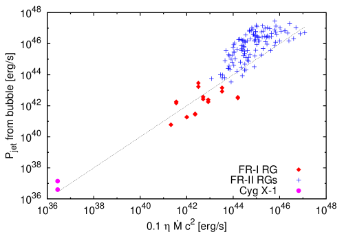
Figure 1: Jet power as a function of the accretion rate. We show the power injected into one jet as a function of the accretion rate as measured from the core radio emission. For Cyg X-1 and FR-I RGs we plot the jet power directly estimated from bubbles. For the FR-II RGs of the 3CRR sample we plot $0.1\eta\dot{M}c^{2}$ for both methods to estimates the accretion rate.

In Fig. 1, we show the jet powers determined for Cyg X-1 and the Allen et al. jets in comparison to our accretion measure. The solid line assumes that the power in one jet is $\approx 1/10$ of the available accretion power. Thus, if the kinetic jet power estimates from bubbles are correct, we find $q_{\mathrm{j}}\approx 0.2$ for the entire twin-jet system. This is consistent with the rough estimate of the jet power given in Körding et al. (2006b). The total jet power can therefore be estimated:

$$P_{jet}\approx 7.2\times 10^{36}\left(\frac{L_{\mathrm{Rad}}}{10^{30}\mbox{erg s}^{-1}}\right)^{12/17}\frac{\mbox{erg}}{\mbox{s}},$$ (2)

Recently, Binney, Bibi & Omma (2007) have reported simulations which indicate that jet powers derived from the pressure and volume of jet bubbles underestimate the true energy input by a factor of order 6. In this case the jets would carry at least half of the power liberated in the accretion disk. The accretion disk could then radiate only half of the accretion power. IF this is correct, all our accretion measure estimates remain applicable, only the jet power and any kinetic power estimate presented below has to be multiplied by a factor 6.

2.2 Accretion rates and jet powers from extended radio emission

2.2.1 Accretion rates

The bulk of the radio luminosity of powerful radio galaxies is emitted by extended lobes with unbeamed, steep-spectrum emission. Rawlings & Saunders (1991) have shown that the strength of this extended emission correlates with the narrow-line luminosity of the optical core. They used the correlation to argue for a common mechanism powering both the radio jets and the optical continuum and line emission. The reality of this correlation has been confirmed by many later studies. In particular, Willott et al. (1999) presented a refined analysis based on complete radio surveys with vastly different flux limits, ruling out distance effects as origin of the correlation. They found a correlation between rest-frame radio power at 151 MHz and narrow-line luminosity, and concluded that the jet power is within one order of magnitude of the radiative power of the accretion disc. As the disc luminosity directly measures the accretion rate, we can use the correlation to determine an accretion rate from 151 MHz radio luminosities for high-power jet sources.

To allow a direct comparison of the ARF generated from these “radio lobe” accretion rates with the ARF derived from the bolometric luminosity of all quasars (i.e., including the majority of quasars without strong radio lobes) by Hopkins et al. (2007), we do not directly use the result of Willott et al. (1999) but renormalize this relation using $B$-band luminosities together with the bolometric corrections of Hopkins et al..

We construct a sample of broad-line quasars with measured 74 MHz radio luminosities by cross-matching quasars from the SDSS DR5 (Schneider et al., 2007) with the VLA Low-frequency Sky Survey VLSS, Cohen et al., 2006, 2007 using a matching radius of 20″ (the histogram of radial separations between the closest matched sources has a local minimum at this matching radius). We use 74 MHz fluxes as this frequency is near the target of 151 MHz, especially for the large number of the quasars around $z\approx 2$, and as the VLSS provides an easily accessible deep survey of the full northern sky. The resulting matched list has a total of 919 entries. We apply the $i$-band emission-line and $K$-correction given in Richards et al. (2006, Table 4) and $K$-correct the VLSS data to 74 MHz rest-frame assuming a spectrum $f_{\nu}\propto\nu^{-0.7}$.

In Fig. 2 we show the 74 MHz luminosity against the absolute $i$-band magnitude. Following the nearly linear correlation between the narrow-line luminosity and the low-frequency radio luminosity found by Willott et al. (1999, see also ()), we fit a linear dependence between the optical $i$-band luminosity (which we assume is proportional to the ionizing luminosity, and hence to the narrow-line luminosity) and the radio luminosity to the data:

$$\log L_{74}=-0.4M_{i}+16.78$$ (3)

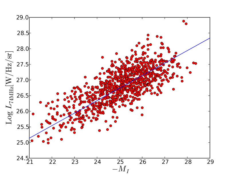
Figure 2: Normalizing the jet power measures from radio luminosities with sources of measured jet powers. On the ordinate ($y$-axis) we plot the 74 MHz radio luminosity and on the abscissa ($x$-axis) we give the absolute $i$-band magnitude. The line represents the linear relation fitted to the data (see text).

To convert the $i$-band magnitudes to $B$-band magnitudes, we assume a power-law spectrum with $\alpha=-0.5$ (see Richards et al., 2006) which yields $B-i=0.3$. For the B-band luminosity we find:

$$\log L_{\mathrm{B}}\left[\frac{\mbox{erg}}{\mbox{s}}\right]\approx\log L_{74}\left[\frac{\mbox{W}}{\mbox{Hz sr}}\right]+18.6.$$ (4)

Throughout this paper we mainly use cgs units. However, as most radio luminosity functions are given in W Hz^-1 sr^-1 we provide the conversion formulae from radio luminosity to accretion rate using these units on the right hand side of the equation. Hopkins et al. (2007) use a non-constant bolometric correction of the $B$-band flux. However, the bolometric correction deviates from a constant mainly at lower luminosities where we will not use the relation to obtain accretion rates. As we would like to obtain a simple relation between the low frequency radio luminosity and the bolometric luminosity we will use a constant bolometric correction of 10, i.e., $L_{bol}\approx 10L_{B}$. Within our uncertainties, this is in agreement with the value used by Hopkins et al. (2007). If we again assume that radio emission has a spectrum $f_{\nu}\propto\nu^{-0.7}$, we can translate the measured relation to:

$$\log L_{\mathrm{bol}}\left[\frac{\mbox{erg}}{\mbox{s}}\right]\approx\log L_{151}\left[\frac{\mbox{W}}{\mbox{Hz sr}}\right]+19.8.$$ (5)

To obtain the accretion rates we assume that the sources are accreting efficiently with a constant efficiency of $\eta=0.1$:

$$\log\dot{M}\left[\frac{\mbox{g}}{\mbox{s}}\right]=\log L_{151}\left[\frac{\mbox{W}}{\mbox{Hz sr}}\right]-0.15$$ (6)

The correlation between optical narrow-line luminosity and 151 MHz radio luminosity (Willott et al., 1999) has only been tested with a sample in the luminosity range of $10^{24.5}\leq L_{\rm 151MHz}/(\mbox{W Hz}^{-1}\mbox{sr}^{-1})\leq 10^{28.8}$. Therefore, we will only use it for extended radio emission brighter than $10^{24.5}$ W Hz^-1.

2.2.2 Jet power

If we assume that the ratio of jet power to accretion rate $q_{\mathrm{j}}$ is similar for hard-state and IMS objects, $q_{\mathrm{j}}\approx 0.2$, we can use the accretion rate determined from the extended low-frequency radio emission also as a measure of the jet power. Willott et al. (1999) and Hardcastle et al. (2007) report that

$$P_{\mathrm{jet}}\left[\frac{\mbox{erg}}{\mbox{s}}\right]\approx 3\times 10^{17}L_{151}\left[\frac{\mbox{W}}{\mbox{Hz sr}}\right]f^{3/2},$$ (7)

where $f$ parameterizes our uncertainty of the jet power compared to the minimum energy needed to account for the synchrotron emission from the lobes. Blundell & Rawlings (2000) suggest that $f\approx 10$ is applicable to FR-II RGs. We find:

$$\log P_{\mathrm{jet}}\left[\frac{\mbox{erg}}{\mbox{s}}\right]\approx 18.7+\log L_{151}\left[\frac{\mbox{W}}{\mbox{Hz sr}}\right].$$ (8)

Our normalization of the $L_{151}$-accretion rate correlation (eq. 5) together with $q_{\mathrm{j}}=0.2$ gives a normalization constant of 19.1 compared to 18.7 as estimated from Willott et al. (1999). The difference corresponds to a factor 2.5. This is well within the uncertainties of our accretion rate and jet power estimates, but may indicate that our normalization is slightly too high.

For the rest of this paper we will assume that the coupling constant of the jet is $q_{\mathrm{j}}=0.2$ and use this to estimate the jet power from the accretion rate for both low-luminosity and high-luminosity objects. Thus, our jet power measure from extended radio emission is:

$$\log P_{\mathrm{jet}}\left[\frac{\mbox{erg}}{\mbox{s}}\right]\approx 19.1+\log L_{151}\left[\frac{\mbox{W}}{\mbox{Hz sr}}\right].$$ (9)

2.3 Comparison of jet and accretion rate measures from both methods

In the preceding subsections we have presented two different accretion rate and jet power measures based on radio luminosities. As we will use these to obtain accretion rate functions, it is important that the estimates are consistent with each other.

To compare the accretion rate measures, we need a sample which has measured values both for the extended low-frequency radio flux and for the unresolved core flux, so that we can compute and compare both accretion rate measures for the same sample. The FR-II radio galaxy subsample of the 3CRR catalogue fulfills these criteria. We take 151 MHz radio fluxes from Laing et al. (1983) and core radio fluxes from the compilation by M. Hardcastle. Since the core fluxes of this sample are probably affected by beaming, we can at the same time assess the impact of beaming.

In Fig. 1 we show the 3CRR FR-II sample together with Cyg X-1 and the Allen et al. (2006) sample of sources with have jet powers inferred from X-ray bubbles. Most of the 3CRR sample lies above the expected line, i.e., the jet power estimated from the extended emission exceeds that estimated from core radio fluxes. While the core flux is affected by beaming, the extended emission is not. For a randomly orientated sample of sources, like the low-frequency selected 3CRR sample, the majority of sources will be deboosted, since they are beamed into a narrow cone (for $\Gamma\gtrsim 1.7$). This explains the lower average jet power estimated from the core.

An additional problem that may alter the relative distribution of the two accretion power estimates is that the extended emission of the lobes can only yield a measure of the jet power averaged over the lifetime of the lobes (several million years). In contrast, the core radio fluxes measures the instantaneous jet power. Thus, if a source changes from having a strong jet to having a quenched jet, but the relativistic particles in the lobes keep radiating for at least a synchrotron lifetime, this will reduce only the core power measure. The reverse effect, i.e., a starting jet, can also happen. However, as the 3CRR sample is selected using low-frequency radio emission those starting sources will not be in the sample.

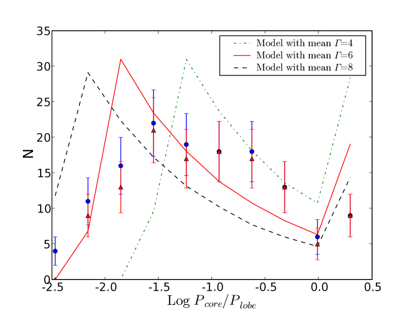
Figure 3: Beaming Statistics of the core radio measure compared to the accretion measure based on the extended emission: On the $x$-axis we show $\log P_{\mathrm{jet,core}}/P_{\mathrm{jet,lobe}}$ while the $y$-axis denotes the number of sources. The filled circles represent the measured histogram including upper limits and the triangles show only those sources with measured core fluxes. The lines describe a beaming model assuming a Gaussian distribution of Lorentz factors around $\Gamma=4,6,8$ with $\sigma=1$.

To verify that the ratios between the core jet power estimate and the lobe jet power estimates are consistent, we show a histogram of the measured ratios in Fig. 3. Some of the sources in the 3CRR catalogue have no measured core radio fluxes. We therefore present two histograms: In the first, we only include detected sources. In the second we include all non-detected sources at their detection limit. In addition to the measured distribution we also present the distribution expected from a randomly orientated sample of relativistic jets. Here, we assume that the observed luminosity is relativistically boosted as $L\sim D^{2.7}L_{0}$, where $L_{0}$ is the luminosity in the rest-frame of the jet and $D$ is the Doppler factor $D=1/[\gamma(1-\beta cos\theta)]$. We have assumed that the Lorentz factors are Gauss-distributed around a Lorentz factor $\Gamma_{0}$ with $\sigma=1$. We show the model for three different mean Lorentz factors: $\Gamma=4,6,8$. While the model assuming $\Gamma=4$ over-predicts the number of boosted objects ($P_{lobe}/P_{core}\geq 1$) it under-predicts the number of strongly deboosted sources. The model assuming $\Gamma=8$ strongly over-predicts the number of deboosted sources. The data is best represented by the model with $\Gamma=6$. This is consistent with the average Doppler factors found in BL Lac objects ($D\sim 7$; Ghisellini et al., 1993). The deviations can be attributed to the simplicity of the model, as well as to short-term changes in the accretion rate which only show in the accretion measure based on the core fluxes. We conclude that both accretion rate measures yield results which are in agreement with each other.

3 Results

We have constructed accretion and jet power measures from radio luminosities. We now use these to translate radio luminosity functions into accretion rate functions and compare those to the measured bolometric luminosity function of quasars (BLF) from Hopkins et al. (2007). For low-luminosity objects we use the local radio luminosity function of Filho et al. (2006). The high-luminosity end is obtained from the low-frequency radio luminosity function of Willott et al. (2001).

3.1 Local accretion rate functions

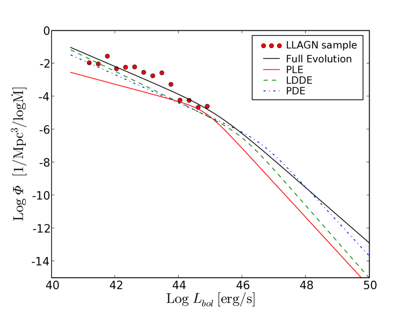
Figure 4: Different models for the cosmological evolution of the bolometric luminosity function extrapolated to $z=0$. The points represent the measured LLAGN radio luminosity function translated to accretion rates. To allow for an easy comparison with the bolometric luminosity function we show the accretion rates as an equivalent bolometric luminosity (0.1 $\dot{M}c^{2}$). To present the uncertainties due to the model of the cosmological evolution we show four different models: Full evolution, PLE, PDE and LDDE. Only the latter model is used in the remainder of this paper.

In Fig. 4 we show the local ARF of LLAGN-like jet sources obtained from our accretion rate measure together with several models of the BLF in the local universe (extrapolated to $z=0$, Hopkins et al. 2007). To compare the ARF with the BLF, we define an equivalent bolometric luminosity $L_{\mathrm{bol}}^{\mathrm{equiv}}=0.1\dot{M}c^{2}$, i.e., we plot the ARF as if the sources were accreting efficiently, with an efficiency of converting rest-mass energy into radiation of $\eta=0.1$. If the majority of the sources in the BLF are indeed accreting efficiently, we can compare the ARF and the BLF directly in this way. This assumption is likely to be true for the high-luminosity quasars. We will discuss the effects of inefficient accretion on the shape of the BLF in section 4.1.

Of the models given in Hopkins et al. (2007), we show the pure luminosity evolution (PLE) model, the pure density evolution (PDE) model, the luminosity dependent density evolution (LDDE) model and the full evolution model. The latter is basically a broken power law model where all parameters (both slopes and the break location) can have a different evolution (for the exact definitions of the different models see the original paper). We show the different models mainly to demonstrate the uncertainties of the modeling and will adopt the LDDE model for the rest of this paper as it currently seems to be the most widely used model and the 151 MHz luminosity function is fitted with an LDDE type model. The BLF has data reaching to $10^{42.1}$ erg/s, below that the models are extrapolated.

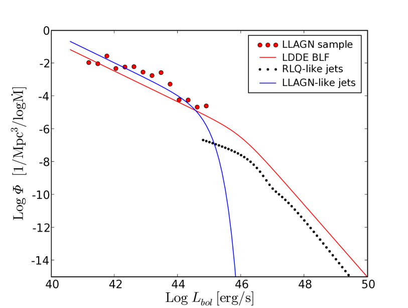
Figure 5: Bolometric luminosity function at $z=0$ ; we also show the measured ARF of “low”-power jet sources (LLAGN-sample) and RLQ-like jet sources (e.g., radio-loud quasars). The latter ARF is obtained from a 151 MHz luminosity function together with eq. (6). The fit to the “low”-power jets is the model of the BLF modified to include an exponential cut-off as seen in the black hole mass function – see text.

Our ARF obtained from the local radio luminosity function is in agreement with the BLF, within the uncertainties of the cosmological evolution. Thus, at low accretion rates there are similar numbers of radio jet-emitting sources and sources appearing in the BLF of Hopkins et al..

Our accretion measure using core radio fluxes is strongly affected by relativistic beaming. However, no AGN below a radio luminosity of $\approx 5\times 10^{22}$ W/Hz shows high apparent velocities (Cohen et al., 2007). This radio luminosity corresponds to a bolometric luminosity of $\approx 2\times 10^{44}$ erg/s. This supports the idea that the low-luminosity radio LF is not strongly affected by relativistic beaming. We mentioned that we expect LLAGN-like jets to exist predominantly below $\sim 2\%$ of the Eddington rate. For a $10^{8}$ M_⊙ BH this corresponds to a bolometric luminosity of $\sim 4\times 10^{44}$ erg s^-1. Thus, LLAGN-like jet are likely to be slower than RLQ-like jets.

The majority of the sources in the low-luminosity radio LF would not be classified as Quasars as they are faint in the optical band and/or do not show broad emission lines. Even though the BLF of Hopkins et al. (2007) is called a “Quasar LF”, it also contains lower-luminosity AGN in addition to Quasars. This partly explains why the ARF of LLAGN-like jets extends the BLF smoothly to lower accretion rates. This will be further discussed in Sect. 4.1.

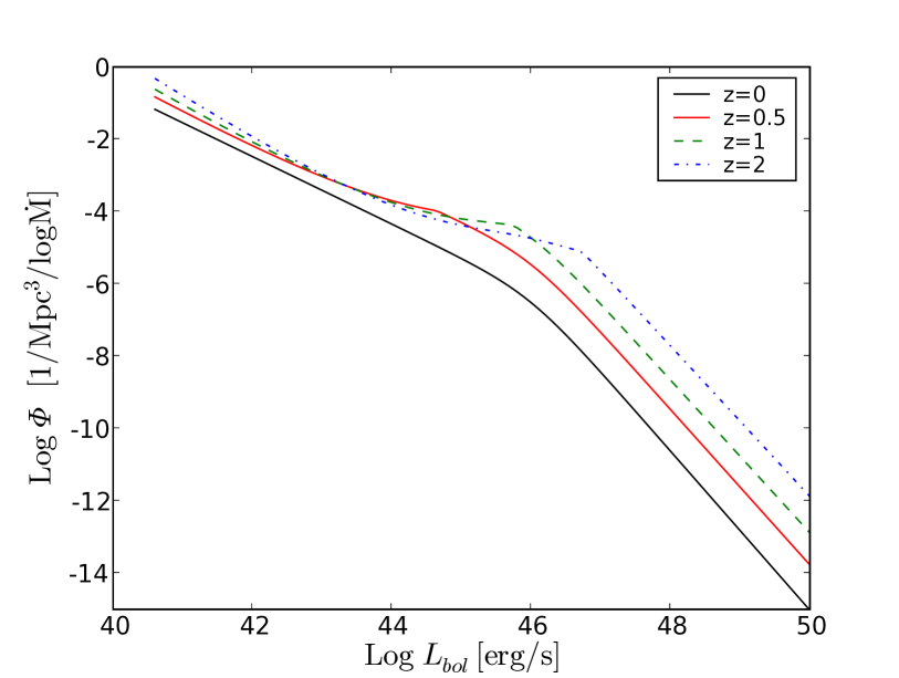
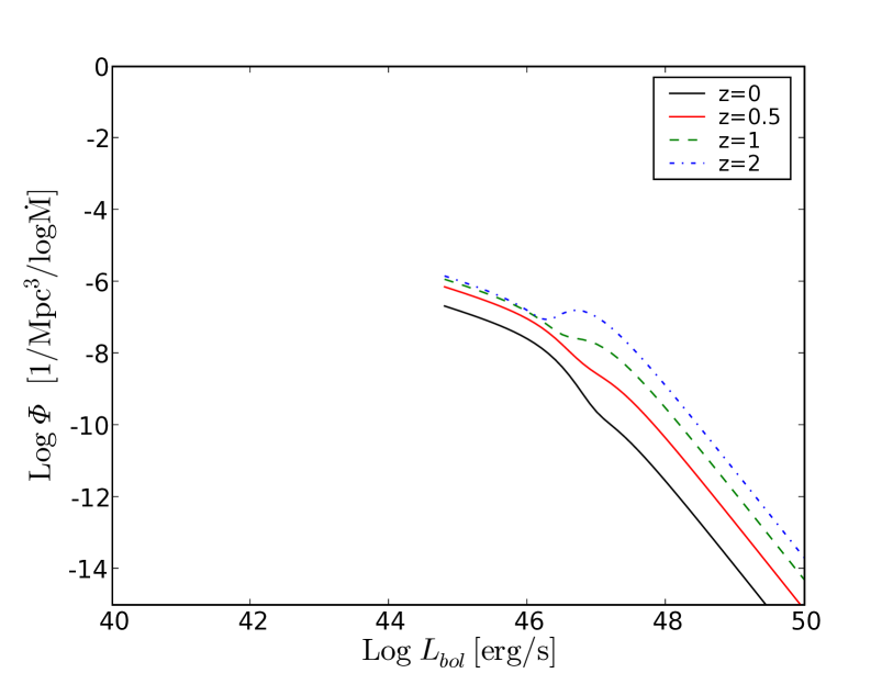
Figure 6: Luminosity function at different redshifts: In the left panel we show the evolution of the BLF at four different redshifts (0,0.5,1,2). This is a reproduction of the LDDE model given in Hopkins et al. (2007) to allow for a direct comparison with the ARF of RLQ-like jets. In the right panel we show the evolution of the ARF of RLQ-like jet sources. The ARF shown is based on the 151 MHz radio LF of Willott et al. (2001).

In Fig. 5 we show the measured ARF of the LLAGN-like jet sources together with the BLF and the ARF deduced from the 151 MHz radio luminosity function. The latter ARF describes the abundance of radio-loud Quasars with lobes, i.e., radio-quiet quasars will not be picked up. While jets of LLAGN-like sources do not seem to be highly relativistic, those of RLQ can be highly relativistic. We will refer to the ARF deduced from the 151 MHz LF also as the luminosity function of “RLQ-like” jets, and we will use the term “strongly jet emitting sources” to refer to all jet-emitting sources, whether the jet is RLQ-like or LLAGN-like. Sources without strong jets will be referred to as radio-quiet.

While the LLAGN-like jet ARF is roughly in agreement with the BLF, the RLQ-like jet ARF lies significantly below it. However, continuity demands that the overall ARF of all jet-emitting sources connects the RLQ-like jet LF smoothly to the LLAGN-like jet ARF. The exact shape of the ARF between the observed domains of LLAGN-like jets and RLQ-like jets is unknown. We attribute the LLAGN-like jet sources to the hard state, which exists predominantly below an accretion rate of $\sim 2\%$ Eddington. For a given accretion rate only black holes above a corresponding minimum mass will have an Eddington ratio below $\sim 2\%$ and always have LLAGN-like jets. Above that Eddington ratio it is likely that the majority of AGN will either show RLQ-like jets or be radio-quiet. Therefore, we can obtain constraints on the ARF of LLAGN-like jet sources from the mass function of supermassive black holes in the local universe.

Shankar et al. (2004) report that the mass function can be described by a power law with an exponential cutoff:

$$\Phi_{\mathrm{BH}}(M)=7.7\times 10^{-3}\left(\frac{M}{M_{*}}\right)^{-0.11}\exp\left[-\left(\frac{M}{M_{*}}\right)^{0.45}\right],$$ (10)

with $M_{*}=6.4\times 10^{7}M_{\odot}$. The BH mass function describes how many BHs can harbour LLAGN-like jets for any given accretion rate. The measured LLAGN-like jet ARF can be well described by a power law – similar to the BH mass function at low BH masses (albeit with a different power law index). As the BH mass function has an exponential cut-off the power law describing the LLAGN-like jet ARF has to cut-off at some point as well. If the majority of AGN with an Eddington ratio larger than $\sim 2\%$ does not show LLAGN-like jets, the BH mass function suggests that the cut-off of the ARF will be the same exponential translated to a luminosity corresponding to $\sim 2\%$ Eddington for BHs with mass $M_{*}$ (this luminosity is $\sim 10^{44.2}$ erg/s). As the LLAGN-like jet ARF is roughly in agreement with the BLF, we therefore describe the LLAGN-like jet ARF with the analytic model of the BLF with an additional exponential cutoff and a constant logarithmic offset. This model with an offset of 0.5 dex is shown in Fig. 5. The total ARF of jet-emitting sources is the sum of both radio ARFs derived from RLQ-like jets and LLAGN-like jets, respectively.

We can now revisit our assumption that the low-luminosity AGN have slow jets. If this assumption was wrong, we would have to correct the luminosity function for beaming. However, we are mainly interested in the low-luminosity end of the radio luminosity function. At the lowest luminosities the beaming correction would in fact increase the total number of sources (see e.g., Lister, 2003). However, the ARF already gives a density of $\sim 10^{-2}$ BHs per Mpc³ and $\log\dot{M}$ for accretion rates below an equivalent bolometric luminosity of $\sim 10^{43}$ erg s^-1. If the beaming correction increased this value significantly (e.g., a factor 10) this would suggest that there were more low-luminosity AGN than BHs in the local universe. Thus, even if there is a small beamed contribution to the luminosity of LLAGN, the beaming correction cannot be strong.

3.2 Redshift evolution of accretion rate functions

In Fig. 6 we show the redshift evolution of the BLF (left-hand panel) and the evolution of the ARF of RLQ-like jet objects (right-hand panel). As the LLAGN-like jet ARF at redshift zero is roughly in agreement with the BLF, we assume that this is also the case for other redshifts. In this case, its cosmological evolution is identical to that of the low-luminosity end of the BLF and we do not show it separately.

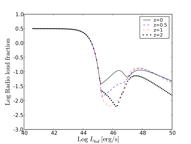
Figure 7: Fraction of radio-loud objects (i.e., volume ratio of radio-loud objects to the BLF) as function of accretion rate for various redshifts (0,0.5,1,2). At low luminosities all sources are likely to be radio-loud. No evolution is visible, as we assume that the radio-loud LLAGN extend the BLF at low luminosities. The evolution at high luminosities is low for moderate redshifts ($z<2$). Only at intermediate luminosities there seems to be a small region showing some evolution. However, this is likely an artifact of the choice of our models. Our accretion rate measures work best at the lowest and highest luminosities.

In Fig. 7 we show the fraction of strongly jet emitting objects for a given accretion rate per volume. The number of strong jet sources is the sum of the number of the LLAGN-like and the RLQ-like jets. At low accretion rates, nearly all sources are radio-loud. The radio ARF is in agreement with the low-luminosity end of the BLF, or lies slightly above it. At the high-luminosity end, the number of RLQ-like jet sources of a given accretion rate is significantly lower than the number of quasars ($\sim 1$ dex). The exact fraction of jet emitting sources is strongly dependent on the normalization of the accretion rate measure based on the extended radio emission. The slope of the BLF is $\sim-2.5$. Thus, all uncertainties in the estimation of the accretion rate enter at least quadratically in the radio-loud fraction. We found in Sect. 2.2.2 that our jet power estimates are slightly higher than those of Willott et al. (1999). If we overestimate the jet power by 0.2 dex, the true fraction of radio-loud objects at high luminosities is less than $3\%$, well in agreement with the values typically found.

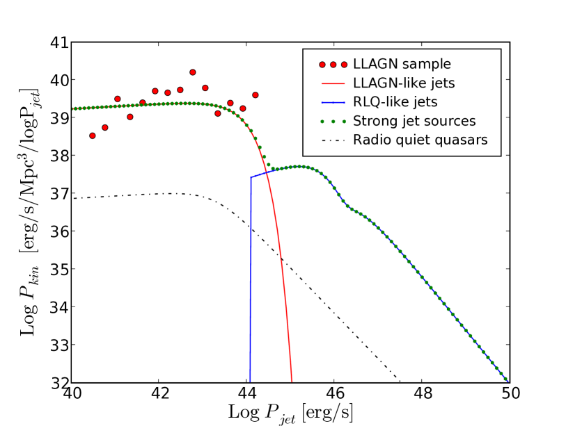
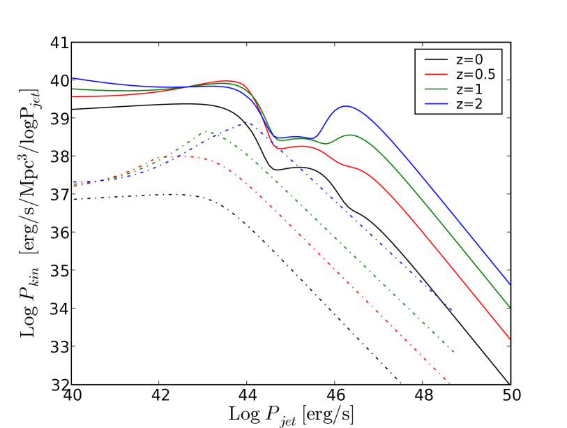
Figure 8: The kinetic luminosity function of jets shows the kinetic power injected into the ISM/IGM per Mpc³ and log${}_{10}P_{\mathrm{jet}}$ as a function of jet power $P_{\mathrm{jet}}$. The left-hand panel shows the different components of the kinetic luminosity function at redshift zero: LLAGN-like jet sources, RLQ-like sources as well as radio-quiet sources. The right-hand panel shows the evolution of the kinetic luminosity function of jet sources (RLQ-like and LLAGN-like jets, solid lines) and radio-quiet sources (dashed lines).

3.3 Jet kinetic luminosity functions

As our accretion measures from radio fluxes are based on the radio emission from the jet, they can also be used as a measure of the jet power (see Fig. 1). Thus, we can compute the kinetic luminosity function (KLF) for jets, i.e., measure how much power is injected into the interstellar or intergalactic medium (ISM/IGM) by jets from sources with a given accretion rate. In sect. 2.2.2, we found that roughly a fraction $q_{\mathrm{j}}=0.2$ of the accretion power is injected into the jet for all jet sources.

In radio-quiet quasars, usually a weak compact core is found. This suggests that there is still an active jet, albeit one of lower power. A typical quenching factor for the radio emission of radio-quiet jets is $\sim 100$ (e.g., Kellermann et al., 1989). If we assume that the radio emission is quenched by a factor 100, the jet powers in in radio-quiet sources (RQQ) are reduced by a factor 30 (assuming $L_{radio}\propto P_{jet}^{1.4}$, e.g., Körding et al. 2006b). We can compare the effect of the RQQ in the KLF to that of RLQs and LLAGN-like jet sources. As the fraction of radio-loud sources is small at high luminosities (a few percent, Fig. 7), the number of radio-quiet sources is approximately the number of all quasars.

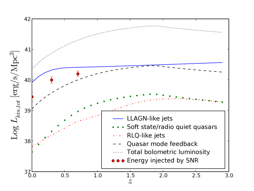
Figure 9: Total kinetic power injected into the ISM at a given redshift by AGN. We show the integrated kinetic energy injected into the IGM by LLAGN, by radio loud quasars and by radio quiet quasars as well as the power available for feedback during the quasar phase (e.g., as radiative feedback). The points denote the kinetic energy injected by supernovae. Additionally, we show the total bolometric luminosity, i.e. the total power liberated through accretion.

The resulting jet KLF is shown in the left-hand panel of Fig. 8. The LLAGN-like jet sources inject significantly more kinetic energy into the ISM than both radio-loud and radio-quiet quasars. The right-hand panel shows that this is true at all redshifts. This can be seen even better in Fig 9, where we plot the total jet power integrated over all accretion rates as a function of redshift. The LLAGN-like jet sources dominate the total kinetic jet power output by an order of magnitude. The contribution of the RLQ-like jet sources is just comparable to those of radio quiet sources. RLQ create jets that are roughly two orders of magnitude stronger than those of the RQQ, but only a few percent of quasars are radio-loud (RLQ-like jet sources). Both factors average out and we find that the contribution of the sample of RQQ and RLQ to the kinetic output is roughly similar.

In addition to the kinetic power injected by AGN, we show the energy available for “quasar-mode” feedback in Fig. 9, assuming that 5 $\%$ of the quasar’s bolometric luminosity is available to heat the surrounding gas (see Di Matteo et al., 2005, e.g.; we discuss the possible nature of the coupling between gas and radiation in sect. 4.2). Even including quasar-mode feedback, the population of low-luminosity AGN with their LLAGN-like jets dominates the total power available for feedback at low redshifts. As the cosmological evolution of the high-luminosity quasars is stronger than for the low-luminosity end, radiative feedback increases in importance until it reaches the same order of magnitude as kinetic feedback at a redshift close to 2. We note that it is not yet possible to observe an LLAGN ARF at $z=1$–$2$. The only hints to the evolution of the low-luminosity radio LF come from the fact that the LLAGN ARF smoothly extends the BLF to lower luminosities, which suggests that one can use evolution of the low-luminosity end of the BLF to estimate the evolution of all LLAGN.

It is now widely accepted that the kinetic energy input from supernovae has a profound impact on the formation and evolution of galaxies (see Efstathiou, 2000, e.g., and references therein). A typical supernova injects around $10^{51}$ erg of kinetic energy into the ambient medium (e.g., Chevalier, 1977; Korpi et al., 1999). Assuming that both core-collapse and type Ia supernovae create a kinetic energy of $10^{51}$ erg, we can estimate the kinetic power injected into the interstellar medium by supernovae, assuming the high-redshift supernova rates estimated from the “Great Observatories Origins Deep Survey” by Dahlen et al. (2004), and compare it to the power created by jets of supermassive black holes. In Fig. 9 we present our power estimate of jets, radiative processes and supernovae. While the contributions of high-power jets (i.e., radio-loud quasars) and radiative processes to the heating of the ambient medium are significantly below the supernova heating rate, LLAGN-like jet sources inject a similar amount of power into the interstellar/intergalactic medium as supernovae. Also the jets of stellar accreting black holes and neutron stars contribute to the kinetic power, albeit at lower rates (e.g., Fender et al., 2005).

Of course, the impact of jets on the galaxy formation process depends critically on the relative magnitude of the jet power, the duration of each jetted phase, the collimation and absolute jet power (see section 4.2), and the binding energy and cooling time of gas in the galaxy. Therefore, it would be highly desirable to derive Fig. 9 separately for different galaxy types, luminosities and black hole masses. This requires knowledge of the radio and bolometric luminosity functions separately for each subcategory, as well as reaching lower luminosities at higher redshifts than is presently possible, and is beyond the scope of this work.

4 Discussion

4.1 The break in the BLF and the missing LLAGN

In Sect. 3.1 we showed that the low-luminosity radio ARF is roughly in agreement with the AGN BLF. However, supermassive black holes at low accretion rate are likely to be radiatively inefficient and would not be classified as a quasar. Assuming the usual high radiative efficiency of quasars will then underestimate the accretion rate. At the lowest luminosities, this suggests that the radio ARF and the BLF should increasingly deviate from each other with decreasing accretion rates, with the radio ARF exceeding the AGN BLF significantly. This is not what we find in the ARFs we have derived (Figures 4 and 5). Here, we explain the observed break in the BLF as due to the onset of inefficient accretion and the “missing” radio LLAGN as due to the fact that there is only a finite number of supermassive BHs.

We have several constraints for modeling the accretion rate function of supermassive black holes. First, the local black-hole mass function has been estimated by Shankar et al. (2004). We can therefore write the accretion rate function as:

$$\Phi(\dot{M})=\int\Phi_{\mathrm{BH}}(M)\bar{\Phi}(M,\dot{M})d\log M,$$ (11)

where $\Phi(\dot{M})$ is the measured accretion rate function in units of Mpc${}^{-3}\ d\log_{10}\dot{M}^{-1}$. Secondly, as the number of AGN integrated over all accretion rates down to 0 has to be equal to the number of all supermassive black holes, it follows:

$$1=\int\bar{\Phi}(M,\dot{M})d\log\dot{M}.$$ (12)

The distribution $\bar{\Phi}(M,\dot{M})$ describes the probability to find a black hole of mass $M$ with an accretion rate $\dot{M}$. In principle that function can be an arbitrary function and there is no unique inversion that obtains $\bar{\Phi}(M,\dot{M})$ from eq. 11 with only the knowledge of $\Phi(\dot{M})$ and $\Phi_{\mathrm{BH}}(M)$. As a first approach, let us assume that the distribution depends only on $\dot{m}$, the accretion rate in Eddington units. This assumption is equivalent with a distribution $\bar{\Phi}(M,\dot{M})$ that separates into a function depending only on $\dot{M}$ and another one depending only on $M$: $\bar{\Phi}(M,\dot{M})=\Phi_{1}(M)\Phi_{2}(\dot{M})$. In astrophysical terms, this assumption means that the Eddington luminosity, i.e., the black-hole mass, sets the total power that is available for feedback from a given black-hole mass, independently of the host galaxy properties.

It is generally assumed that strongly accreting objects are radiatively efficient. As the BLF is well-described by a power law at high luminosities (above the break), it is likely that the distribution $\bar{\Phi}(\dot{m})$ is a power law at high Eddington ratios. However, as the power-law index of the luminosity function is steep ($\sim-2$), it has to have a cut-off towards low luminosities so that its integral does not diverge. As there are known strongly sub-Eddington sources (e.g., Sgr A^∗), a hard cut-off would not be appropriate, and we use a broken power law of the form:

$$\bar{\Phi}(\dot{m})\propto\left\{\begin{array}[]{ll}\dot{m}^{\gamma_{2}}&\mbox{for}\ \dot{m}_{\mathrm{break}}\leq\dot{m}\\ \left(\dot{m}/\dot{m}_{\mathrm{break}}\right)^{\gamma_{1}}\dot{m}^{\gamma_{2}}_{\mathrm{break}}&\mbox{for}\ \dot{m}\leq\dot{m}_{\mathrm{break}}.\end{array}\right.$$ (13)

As the function has to be integrable with respect to $d\log\dot{m}$ we require $\gamma_{1}\geq 0$. At high accretion rates, we truncate the power law at 10 Eddington rates. The distribution will be normalized according to eq. (12).

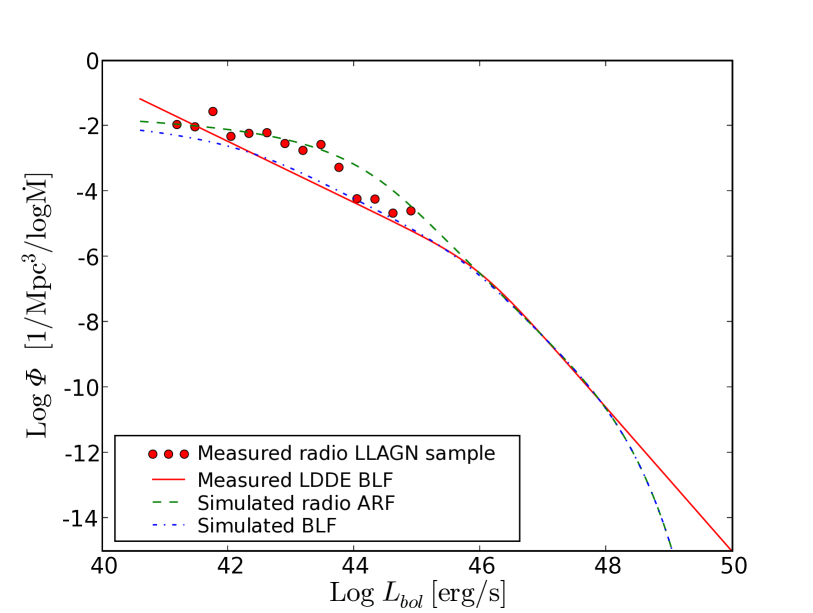
Figure 10: Measured ARF and BLF together with our model for the LFs. While the model for the ARF assumes that the accretion rate is directly measured we assume inefficient accretion below a critical accretion rate for the simulated BLF. We can reproduce both, the ARF and the BLF with our simple model.

While the ARF obtained from the radio estimates should directly measure $\Phi(\dot{M})$, the bolometric luminosity depends linearly on the accretion rate only for the high-accretion rate sources. For strongly sub-Eddington sources we have to translate the accretion rate to a bolometric luminosity. The analogy of AGN to XRBs suggests that the bolometric luminosity of an accreting BH can be described as:

$$L_{\mathrm{bol}}=\left\{\begin{array}[]{ll}L_{\mathrm{Edd}}\;\dot{m}&\mathrm{for}\ \dot{m}\geq\dot{m}_{\mathrm{crit}}\\ L_{\mathrm{Edd}}\;\dot{m}_{\mathrm{crit}}\left(\frac{\dot{m}}{\dot{m}_{\mathrm{crit}}}\right)^{2}&\mathrm{for}\ \dot{m}<\dot{m}_{\mathrm{crit}}\end{array}\right.$$ (14)

where $\dot{m}$ is the accretion rate in Eddington units and $\dot{m}_{\mathrm{crit}}\approx 0.05$. Note that the $\dot{m}_{\mathrm{break}}$ used in the previous paragraph has no direct relation to $\dot{m}_{\mathrm{crit}}$. The exact value of $\dot{m}_{\mathrm{crit}}$ seems to be different for the rise of each XRB outburst $(0.03\leq\dot{m}_{\mathrm{crit}}\leq 0.3)$. On the decline it seems to be more stable $(\dot{m}_{\mathrm{crit}}\sim 0.02)$. For our simple model we will use a constant critical accretion rate of $\dot{m}_{\mathrm{crit}}\sim 0.05$.

We can now combine the measured supermassive black hole function (eq. 10) with our assumptions about the accretion rate distribution (eq. 13) to obtain an accretion rate function, $\Phi(\dot{M})$. This function can be compared directly to the ARFs obtained from the radio emission. To obtain a BLF we include the description given in eq. 14 to translate from accretion rates to luminosities for sources of a given mass. The free parameters are $\gamma_{1,2}$ and the break ($\dot{m}_{\mathrm{break}}$) in the power-law distribution of $\dot{m}$, and to some extent the critical accretion rate $\dot{m}_{\mathrm{crit}}$. The latter is constrained from the observations of XRBs and the finding that this value seems to be similar in AGN (Jester, 2005; Körding et al., 2006b).

In this paper we only try to explain the small difference between the measured radio ARF and the BLF at low luminosities. Thus, we will not explicitly find a best-fit model to the data, but only compare a plausible model to the ARF and the BLF.

The high-luminosity slope of the ARF and the BLF is mainly affected by the power-law index $\gamma_{2}$ at high accretion rates. The position of the break in the accretion rate distribution ($\dot{m}_{\mathrm{break}}$) strongly affects the normalization of the BLF. If the break is too low, most BHs have a very low $\dot{m}$ and there are not enough bright quasars. Thus, both $\gamma_{2}$ and $\dot{m}_{\mathrm{break}}$ can be estimated from the high-luminosity end of the BLF above the break. The low-luminosity index $\gamma_{1}$ has a rather minor effect on both the ARF and the BLF as long as $\gamma_{1}>0$. In Fig. 10 we show the local radio ARF and the BLF together with one realization of our model ($\gamma_{2}=-1.9$, $\dot{m}_{\mathrm{break}}=2\times 10^{-3}$, and $\gamma_{1}=1$). Both the BLF and the radio ARF are reproduced.

The features in the BLF and ARF can be understood as follows. The break in the BLF is created by radiative inefficiency at low accretion rates (this effect of radiative inefficiency on the luminosity function of AGN was exploited by Jester 2005 to look for inefficiency in AGN). The flattening of the ARF at lower luminosity is due to the finite number of supermassive black holes – if the ARF did not flatten, there would need to be more low-luminosity AGN, not leaving enough black holes to account for the observed high-luminosity (quasar) population.

With the simple assumption that the distribution function of accretion rates $\bar{\Phi}(\dot{m})$ depends only on the accretion rate in Eddington units and can be described with a broken power law we seems to be able to reproduce the observed LFs. However, there are several suggestions that the distribution does depend on the black hole mass (e.g., Allen et al., 2006). If we relax our assumption that the distribution function $\bar{\Phi}(M,\dot{M})$ separates into distribution for the accretion rate and one for the black hole mass, we have enormous freedom to choose the distribution. We tried several functions, e.g., we explored if the break of the broken power law in the $\dot{m}$ distribution can depend on the mass, but were not able to improve the fits significantly above the simple model we presented.

Hopkins et al. (2006a) model the quasar luminosity function by considering the birth rate of quasars with a given peak luminosity and the subsequent evolution of the quasar light curve in their merger-driven model. They explain the break in the LF as a characteristic luminosity at which the birth rate peaks. Hopkins et al. (2006b) examine the evolution of the light curves in more detail and show that quasar light curves vary systematically with peak luminosity, i.e., an individual black hole’s accretion rate evolution depends on the peak accretion rate. In the framework of these models, $\bar{\Phi}(\dot{m})$ will vary with redshift depending on the age distribution and lightcurves of currently active black holes, and possibly in different ways from the variation we would require. A detailed comparison between our and the Hopkins et al. models woudld require knowledge of the high-redshift black-hole mass and LLAGN luminosity functions, which are however not yet available.

We note that our model suggests that the weakest LLAGN do not only have a small central BH but should also be fed at a strongly sub-Eddington (and even sub-Bondi) accretion rate (Yuan et al., 2003; Cuadra et al., 2006; Marrone et al., 2007, see, e.g., the simulations and model-fitting for Sgr A^∗ [).

4.2 Implications for feedback

4.2.1 Available feedback power as function of accretion rate

In sect. 3.3 we have confirmed earlier findings that AGN at lower luminosities (e.g., LINERs and low-luminosity FR-I RGs) are likely to dominate the total kinetic power output in the local universe with their LLAGN-like jets (Best et al., 2006; Heinz et al., 2007). Their total kinetic power is comparable to the power injected into the ISM by supernovae. The population of jets in radio-loud and quiet quasars carry more than an order of magnitude less power than the jets of low-luminosity AGN; in fact their total power is not much greater than that injected by jets of XRBs. At higher redshifts the power injected into the IGM by quasars increases more strongly than the power injected by the lower-luminosity objects. However, the low-luminosity objects still seem to dominate. If a fixed fraction of the luminosity of quasars is available for feedback even in the absence of strong jets (e.g. by direct radiative heating or via radiation pressure-driven winds), feedback from luminous quasars also increases with redshift. For a feedback fraction of 5%, this “quasar mode” would make a significant contribution to the total power available for feedback at redshifts close to 2, and even dominate the total feedback for fractions larger than 5%. This is certainly only true when summing over the entire population of all supermassive black holes; a different scenario is likely to be found in the center of clusters and in individual galaxies. Again, we stress that radio and bolometric luminosity extending to lower luminosities, higher redshifts, and separated by host galaxy type, are needed to assess the impact of feedback separately for galaxies of different galaxy type, luminosity, or black hole mass.

Nevertheless, from the models used to explain the measured radio accretion rate function, kinetic power function and the bolometric luminosity, we can deduce feedback properties of individual objects. The analogy of AGN with XRBs and our explanation of the break in the quasar LF in the preceding section suggest that all accreting black holes below a critical accretion rate around $3\times 10^{-2}$ of the Eddington rate are accreting inefficiently and in a jet-dominated mode. Above that critical accretion rate, a source can either be in the hard or hard intermediate state and continue to be strongly jet emitting, or the jet power is quenched by a factor $\sim 30$. With the efficiencies discussed above, we obtain the following approximations for the kinetic power available for feedback, as function of the fundamental parameters $\dot{m}$ and $L_{\mathrm{Edd}}$, i.e., $M_{\mathrm{BH}}$:

$$P_{\mathrm{kin}}=\left\{\begin{array}[]{ll}0.2\,\dot{m}\,L_{\mathrm{Edd}}&\mbox{if}\ \dot{m}\leq\dot{m}_{\mathrm{crit}}\\ 0.2\,\epsilon_{\mathrm{FR-II}}\,\dot{m}\,L_{\mathrm{Edd}}&\mbox{if}\ \dot{m}>\dot{m}_{\mathrm{crit}},\ \mbox{with jet}\\ 0.007\,\dot{m}\,L_{\mathrm{Edd}}&\mbox{if}\ \dot{m}>\dot{m}_{\mathrm{crit}},\ \mbox{no jet}\end{array}\right.$$ (15)

The “with jet” and “no jet” cases refer to radio-quiet quasars and radio-loud quasars/radio galaxies, respectively. For the latter category, it is unlikely that much of the power in the jet will be deposited inside the galaxy, as essentially all the energy is transported out into the lobes which can be located anything from tens of kiloparsecs to a few Megaparsecs away from the central galaxy. The additional efficiency factor $\epsilon_{\mathrm{FR-II}}$ accounts for this effect.

It is not yet certain if and how radio-quiet quasars actually provide energy to heat the ambient medium. One possibility is that a certain fraction of the bolometric luminosity couples to the gas through line driving (e.g., Fabian et al., 2006). Another possibility is that the quasar launches a wind that heats the gas through its kinetic power. It is likely that this process is also linearly coupled to the bolometric luminosity. According to the model used in this paper, low accretion-rate objects are inefficiently accreting up to the critical accretion rate. Accretion above that rate is radiatively efficient. The approximate dependence of the bolometric luminosity on accretion rate is given in eq. (14). It has been argued that roughly 5$\%$ of the bolometric luminosity is available to heat the surrounding gas (e.g., Di Matteo et al., 2005). We will use this model to compare the effects of radiative feedback to the kinetic heating due to jets, i.e., the radiative feedback is given by

$$P_{\mathrm{radfeed}}=0.05L_{\mathrm{bol}}.$$ (16)

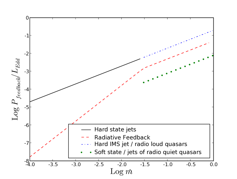
Figure 11: Power available for feedback as function of accretion rate, both in Eddington units (from eqns. 15 and 16). Sources are kinetically dominated at low accretion rates, but radiative feedback may dominate at high accretion rates. A simple linear dependency may correctly describe the total available power as function accretion rate within measurement uncertainties.

Figure 11 shows the power available from a single source (eqns. 15 and 16) via both feedback mechanisms, radiative and kinetic (setting $\epsilon_{\mathrm{FR-II}}=1$ for jet-active radio-loud quasars/radio galaxies), as function of accretion rate. At low accretion rates, the kinetic feedback of the jet dominates the total power output. At high accretion rates, the radiative feedback is efficient and contributes significantly to the total power. The jet is either quenched and the power in the jet is negligible compared to the power available via radiative feedback – or the source is still jet-active and radiative and kinetic feedback are comparable for our parameters. If most of the energy in the jet is injected into distant lobes and not deposited inside the galaxy and $\epsilon_{\mathrm{FR-II}}\ll 1$, as is very likely the case, the kinetic feedback of radio-loud quasars is actually much lower than the maximum available feedback energy shown in our figures.

At low accretion rates, the total power available for feedback is linearly dependent on the accretion rate and dominated by the kinetic power of the jets. At high accretion rates, the total power is either dominated by radiative feedback, or a combination of radiative and kinetic power. Again, the total feedback depends linearly on the accretion rate with a proportionality factor similar to that in the hard state. Thus, the assumption that the energy available for feedback is roughly $P_{\mathrm{feedback}}\sim 0.01\dot{M}c^{2}$, seems to be correct within a factor 2 for all accretion rates; i.e., $P_{\mathrm{feedback}}$ is 10% of $0.1\dot{M}c^{2}$, the power liberated by the accretion process.

4.2.2 Total jet feedback may exceed total supernova feedback

As mentioned, Binney et al. (2007) have suggested recently that the jet power estimates from bubbles underestimate the total jet power by a factor of order 6. In this case, all jet lines in Fig. 11 move up by a factor 6. The jet power would then be an order of magnitude above the power available via radiative feedback. Strongly jet emitting-sources (including both LLAGN and FR-II radio galaxies and quasars) would have significantly more power available for feedback than radio-quiet objects. As a population, LLAGN-like jet sources would inject significantly more power into the ISM than the kinetic power created by all supernovae.

5 Summary and conclusion

For both AGN and X-ray binaries, both the accretion rate and the jet power can be estimated from either the core radio luminosity (Körding et al., 2006b) or the extended low-frequency radio luminosity (Willott et al., 1999). Using these accretion rate estimates, we construct accretion rate functions (ARFs) of jet-emitting sources. The luminosity function (LF) of low-luminosity sources – which likely have slow jets – is roughly in agreement with the bolometric luminosity function (BLF) of AGN (Fig. 4) as determined by Hopkins et al. (2007). The ARF of RLQ-like jet sources is roughly 1 dex below the BLF (Fig. 7). This provides a measurement of the radio-loud fraction with a direct physical meaning: the ratio of volume densities of radio-loud and radio-quiet sources at a given accretion rate. However, the exact value is unfortunately strongly dependent on the normalizations used to derive accretion rates.

We have developed a simple model based on the universality of accretion physics in XRBs and AGN that reproduces both our ARF as well as the BLF. At low luminosities, all sources are radiatively inefficient and the luminosity depends quadratically on the accretion rate (eq. 14). Sources are radiatively efficient only at high luminosities ($\ga 3\%$ Eddington). In our model, we assumed that the distribution of accretion rates does not depend on the black-hole mass and can be written as a simple broken power law for the Eddington-scaled accretion rate (eq. 13). With this model we can reproduce the measured ARF as well as the local BLF (Fig. 10). Thus, this model can solve the problem that there seem to be too few LLAGN compared to the number of weak quasars. In this simple model the break in the luminosity function is due to the inefficient accretion at low accretion rates (compare Jester, 2005).

Using the corresponding jet power measures, we have calculated kinetic luminosity functions and their cosmological evolution. Our findings support the idea that the majority of the kinetic power is created by lower-luminosity AGN with their likely slow jets. The highly luminous radio-loud quasars do not contribute significantly due to their low number density. The total power injected into the ambient medium by jets from AGN is comparable or even exceeds the effect of supernovae (the situation may and will be different for individual objects). Only at high redshifts, “quasar-mode” feedback mechanisms provide a comparable amount of energy for heating the interstellar/intergalactic gas. Finally, we discuss the effects of the different feedback mechanisms and find that a roughly constant fraction (5-10$\%$) of the accretion power is available for feedback, independent of the nature of the AGN.

References

- Allen et al. (2006) Allen S. W., Dunn R. J. H., Fabian A. C., Taylor G. B., Reynolds C. S., 2006, MNRAS, 372, 21
- Belloni et al. (2005) Belloni T., Homan J., Casella P., van der Klis M., Nespoli E., Lewin W. H. G., Miller J. M., Méndez M., 2005, A&A, 440, 207
- Best et al. (2006) Best P. N., Kaiser C. R., Heckman T. M., Kauffmann G., 2006, MNRAS, 368, L67
- Binney et al. (2007) Binney J., Bibi F. A., Omma H., 2007, MNRAS, 377, 142
- Binney & Tabor (1995) Binney J., Tabor G., 1995, MNRAS, 276, 663
- Blundell & Rawlings (2000) Blundell K. M., Rawlings S., 2000, AJ, 119, 1111
- Chevalier (1977) Chevalier R. A., 1977, ARA&A, 15, 175
- Chiaberge et al. (2006) Chiaberge M., Gilli R., Macchetto F. D., Sparks W. B., 2006, ApJ, 651, 728
- Churazov et al. (2001) Churazov E., Brüggen M., Kaiser C. R., Böhringer H., Forman W., 2001, ApJ, 554, 261
- Cohen et al. (2007) Cohen A. S., Lane W. M., Cotton W. D., Kassim N. E., Lazio T. J. W., Perley R. A., Condon J. J., Erickson W. C., 2007, AJ, 134, 1245
- Cohen et al. (2006) Cohen A. S., Lane W. M., Kassim N. E., Lazio T. J. W., Cotton W. D., Perley R. A., Condon J. J., Erickson W. C., 2006, Astronomische Nachrichten, 327, 262
- Cohen et al. (2007) Cohen M. H., Lister M. L., Homan D. C., Kadler M., Kellermann K. I., Kovalev Y. Y., Vermeulen R. C., 2007, ApJ, 658, 232
- Corbel et al. (2000) Corbel S., Fender R. P., Tzioumis A. K., Nowak M., McIntyre V., Durouchoux P., Sood R., 2000, A&A, 359, 251
- Cowie & Binney (1977) Cowie L. L., Binney J., 1977, ApJ, 215, 723
- Cuadra et al. (2006) Cuadra J., Nayakshin S., Springel V., di Matteo T., 2006, MNRAS, 366, 358
- Dahlen et al. (2004) Dahlen T., et al., 2004, ApJ, 613, 189
- Di Matteo et al. (2005) Di Matteo T., Springel V., Hernquist L., 2005, Nature, 433, 604
- Efstathiou (2000) Efstathiou G., 2000, MNRAS, 317, 697
- Esin et al. (1997) Esin A. A., McClintock J. E., Narayan R., 1997, ApJ, 489, 865+
- Fabian et al. (2006) Fabian A. C., Celotti A., Erlund M. C., 2006, MNRAS, 373, L16
- Falcke et al. (2004) Falcke H., Körding E., Markoff S., 2004, A&A, 414, 895
- Fender et al. (1999) Fender R., et al., 1999, ApJ, 519, L165
- Fender (2001) Fender R. P., 2001, MNRAS, 322, 31
- Fender et al. (2004) Fender R. P., Belloni T. M., Gallo E., 2004, MNRAS, 355, 1105
- Fender et al. (2003) Fender R. P., Gallo E., Jonker P. G., 2003, MNRAS, 343, L99
- Fender et al. (2005) Fender R. P., Maccarone T. J., van Kesteren Z., 2005, MNRAS, 360, 1085
- Filho et al. (2006) Filho M. E., Barthel P. D., Ho L. C., 2006, A&A, 451, 71
- Gallo et al. (2005) Gallo E., Fender R., Kaiser C., Russell D., Morganti R., Oosterloo T., Heinz S., 2005, Nature, 436, 819
- Gallo et al. (2003) Gallo E., Fender R. P., Pooley G. G., 2003, MNRAS, 344, 60
- Ghisellini et al. (1993) Ghisellini G., Padovani P., Celotti A., Maraschi L., 1993, ApJ, 407, 65
- Giovannini et al. (2005) Giovannini G., Taylor G. B., Feretti L., Cotton W. D., Lara L., Venturi T., 2005, ApJ, 618, 635
- Gleissner et al. (2004) Gleissner T., et al., 2004, A&A, 425, 1061
- Haehnelt et al. (1998) Haehnelt M. G., Natarajan P., Rees M. J., 1998, MNRAS, 300, 817
- Hardcastle et al. (2007) Hardcastle M. J., Evans D. A., Croston J. H., 2007, MNRAS, 376, 1849
- Heinz & Merloni (2004) Heinz S., Merloni A., 2004, MNRAS, 355, L1
- Heinz et al. (2007) Heinz S., Merloni A., Schwab J., 2007, ApJ, 658, L9
- Ho (1999) Ho L. C., 1999, ApJ, 516, 672
- Homan & Belloni (2005) Homan J., Belloni T., 2005, Ap&SS, 300, 107
- Hopkins et al. (2006a) Hopkins P. F., Hernquist L., Cox T. J., Di Matteo T., Robertson B., Springel V., 2006a, ApJS, 163, 1
- Hopkins et al. (2006b) Hopkins P. F., Hernquist L., Cox T. J., Robertson B., Di Matteo T., Springel V., 2006b, ApJ, 639, 700
- Hopkins et al. (2007) Hopkins P. F., Richards G. T., Hernquist L., 2007, ApJ, 654, 731
- Ichimaru (1977) Ichimaru S., 1977, ApJ, 214, 840
- Jester (2005) Jester S., 2005, ApJ, 625, 667
- Kellermann et al. (1989) Kellermann K. I., Sramek R., Schmidt M., Shaffer D. B., Green R., 1989, AJ, 98, 1195
- King (2003) King A., 2003, ApJ, 596, L27
- Körding et al. (2006a) Körding E., Falcke H., Corbel S., 2006a, A&A, 456, 439
- Körding et al. (2006b) Körding E. G., Fender R. P., Migliari S., 2006b, MNRAS, 369, 1451
- Körding et al. (2006c) Körding E. G., Jester S., Fender R., 2006c, MNRAS, 372, 1366
- Korpi et al. (1999) Korpi M. J., Brandenburg A., Shukurov A., Tuominen I., 1999, A&A, 350, 230
- Laing et al. (1983) Laing R. A., Riley J. M., Longair M. S., 1983, MNRAS, 204, 151
- Lister (2003) Lister M. L., 2003, ApJ, 599, 105
- Livio et al. (2003) Livio M., Pringle J. E., King A. R., 2003, ApJ, 593, 184
- Maccarone (2003) Maccarone T. J., 2003, A&A, 409, 697
- Maccarone et al. (2003) Maccarone T. J., Gallo E., Fender R., 2003, MNRAS, 345, L19
- Maraschi & Tavecchio (2003) Maraschi L., Tavecchio F., 2003, ApJ, 593, 667
- Marrone et al. (2007) Marrone D. P., Moran J. M., Zhao J.-H., Rao R., 2007, ApJ, 654, L57
- Marulli et al. (2007) Marulli F., Branchini E., Moscardini L., Volonteri M., 2007, MNRAS, 375, 649
- Massey et al. (1995) Massey P., Johnson K. E., Degioia-Eastwood K., 1995, ApJ, 454, 151
- McClintock & Remillard (2006) McClintock J., Remillard R., 2006, in ”Compact Stellar X-ray Sources,” eds. W.H.G. Lewin and M. v an der Klis, Cambridge University Press
- McHardy et al. (2006) McHardy I. M., Koerding E., Knigge C., Uttley P., Fender R. P., 2006, Nature, 444, 730
- Meier (2001) Meier D. L., 2001, ApJ, 548, L9
- Merloni et al. (2003) Merloni A., Heinz S., Di Matteo T., 2003, MNRAS, 345, 1057
- Mirabel & Rodriguez (1998) Mirabel I. F., Rodriguez L. F., 1998, Nature, 392, 673
- Nagar et al. (2005) Nagar N. M., Falcke H., Wilson A. S., 2005, A&A, 435, 521
- Nowak (1995) Nowak M. A., 1995, PASP, 107, 1207+
- Rawlings & Saunders (1991) Rawlings S., Saunders R., 1991, Nature, 349, 138
- Rees et al. (1982) Rees M. J., Phinney E. S., Begelman M. C., Blandford R. D., 1982, Nature, 295, 17
- Richards et al. (2006) Richards G. T., et al., 2006, AJ, 131, 2766
- Robertson et al. (2006) Robertson B., Hernquist L., Cox T. J., Di Matteo T., Hopkins P. F., Martini P., Springel V., 2006, ApJ, 641, 90
- Russell et al. (2007) Russell D. M., Fender R. P., Gallo E., Kaiser C. R., 2007, MNRAS, 376, 1341
- Schneider et al. (2007) Schneider D. P., et al., 2007, AJ, 134, 102S
- Shakura & Sunyaev (1973) Shakura N. I., Sunyaev R. A., 1973, A&A, 24, 337
- Shankar et al. (2004) Shankar F., Salucci P., Granato G. L., De Zotti G., Danese L., 2004, MNRAS, 354, 1020
- Silk & Rees (1998) Silk J., Rees M. J., 1998, A&A, 331, L1
- Stirling et al. (2001) Stirling A. M., Spencer R. E., de la Force C. J., Garrett M. A., Fender R. P., Ogley R. N., 2001, MNRAS, 327, 1273
- Volonteri et al. (2006) Volonteri M., Salvaterra R., Haardt F., 2006, MNRAS, 373, 121
- Willott (2001) Willott C. J., 2001, in Rocca-Volmerange B., Sol H., eds, EAS Publications Series Radio-optical correlations in high-z radio galaxies and quasars. pp 109–118
- Willott et al. (1999) Willott C. J., Rawlings S., Blundell K. M., Lacy M., 1999, MNRAS, 309, 1017
- Willott et al. (2001) Willott C. J., Rawlings S., Blundell K. M., Lacy M., Eales S. A., 2001, MNRAS, 322, 536
- Yuan et al. (2003) Yuan F., Quataert E., Narayan R., 2003, ApJ, 598, 301