Operator Methods, Abelian Processes and Dynamic Conditioning

Abstract.

A mathematical framework for Continuous Time Finance based on operator algebraic methods offers a new direct and entirely constructive perspective on the field. It also leads to new numerical analysis techniques which can take advantage of the emerging massively parallel GPU architectures which are uniquely suited to execute large matrix manipulations.

This is partly a review paper as it covers and expands on the mathematical framework underlying a series of more applied articles. In addition, this article also presents a few key new theorems that make the treatment self-contained. Stochastic processes with continuous time and continuous space variables are defined constructively by establishing new convergence estimates for Markov chains on simplicial sequences. We emphasize high precision computability by numerical linear algebra methods as opposed to the ability of arriving to analytically closed form expressions in terms of special functions. Path dependent processes adapted to a given Markov filtration are associated to an operator algebra. If this algebra is commutative, the corresponding process is named Abelian, a concept which provides a far reaching extension of the notion of stochastic integral. We recover the classic Cameron-Dyson-Feynman-Girsanov-Ito-Kac-Martin theorem as a particular case of a broadly general block-diagonalization algorithm. This technique has many applications ranging from the problem of pricing cliquets to target-redemption-notes and volatility derivatives. Non-Abelian processes are also relevant and appear in several important applications to for instance snowballs and soft calls. We show that in these cases one can effectively use block-factorization algorithms. Finally, we discuss the method of dynamic conditioning that allows one to dynamically correlate over possibly even hundreds of processes in a numerically noiseless framework while preserving marginal distributions.

1. Introduction

The goal of this paper is to attempt to consolidate and present a number of mathematical methods developed over several years by myself and collaborators while addressing concrete problems in derivative pricing theory. The results scattered across a number of papers which are collected here have been complemented with a rigorous ab initio treatment and a few key theorems which make the framework mathematically self-contained. This results in a quite comprehensive approach to the theory of Stochastic Processes and Mathematical Finance which is novel in that it is fully constructive and perhaps has applications beyond the realm of Financial Engineering.

There are several traditions of Constructive Mathematics. One attempts to re-derive classical results of real and functional analysis based on a restrictive constructivist logic according to which no mathematical object can be considered unless one specifies explicitly how to construct it, see [BR1987] and [Bishop1967]. Along another tradition, Constructive Field Theory, see [GJ1987], aimed at establishing the existence of interacting quantum field theories by providing a constructive procedure for computing $n$-point functions and demonstrating that they satisfy a set of axioms. Measure theoretic probability and the related theory of stochastic processes, [Doob1953], does not seem to be understandable constructively. The PDE approach in [Feller] and the harmonic analysis approach in [Bochner1987] are instead essentially constructive but do not delve into the theory of stochastic integrals and path dependent processes and into lattice discretization schemes.

The main motivation that guided this research is the creation of an engineering framework for exotic financial derivatives. Efficient computability on current hardware has been and remains throughout this article our key motivating concern. To this end, we work towards an algebraization of Probability Theory that reduces all calculations to matrix manipulations which can be performed efficiently and in particular to matrix multiplications. Similarly to the standard framework of algebraic topology, [Spanier1966], we consider processes taking values in separable topological spaces and approximate continuous domains by means of simplicial sequences. To establish convergence in the continuous limit, we directly estimate convergence rates for probability transition kernels in the continuous space limit following an approach similar in spirit to Constructive Lattice Field Theory, see [GJ1987]. Similarly to constructive field theory, sets of axioms on $n$-point functions are used to identify processes and renormalization group transformations are used to control the continuous limit. Following [Naimark1959], the approach is grounded upon the algebraic theory of integration on locally compact Hausdorff separable topological spaces.

Calculations with stochastic processes are carried out using operator methods developed in Quantum Mechanics, [LandauLifshits] and systematized in Mathematical Physics references such as [ReedSimon]. In Finance, operator methods have been developed along two independent and non-overlapping streams of research, one by Ait-Sahalia, Hansen and Scheinkman who focused on econometric estimations in a series of papers reviewed in [AHS2005], see also [Ait-Sahalia96], [HST98], [HS95]. The second stream of research is by the author and collaborators who instead worked on derivative pricing for path dependent and correlation derivatives, see [ACDV], [AChen4], [AChen5], [AKusnetsov5], [AL2004], [ALoMijatovic], [ATrovato3], [ATrovato2], [AVidler], [AJones] and [AOsseiran]. In this paper, we attempt to systematize the mathematical framework of pricing theory in the operator formalism from our own viewpoint, reserving to future work the task of pursuing overlaps with the econometric literature.

The references quoted above are all relevant to our undertaking and provided motivations on many levels. However, in an effort to keep this writing self-contained, we are not going to assume any previous knowledge of the reader.

To ground the mathematical framework, we obtain sharp pointwise convergence estimates for probability kernels and its derivatives. More precisely, we show that probability kernels converge pointwise at rates of order $O(h^{2})$, where $h$ is the lattice spacing. The result applies to a large class of diffusion processes and extensions thereof including smooth space inhomogeneities, regime switching, finite activity jumps and some degree of time inhomogeneities. We also prove similar convergence results for the fast exponentiation method, our preferred numerical method for exponentiating Markov generators, showing that errors in this scheme are also of order $O(h^{2})$, in the sense of pointwise convergence for the probability kernel. In the particular case of Brownian motion, we show that similar $O(h^{2})$ pointwise error estimates apply also to derivatives of the probability kernels and that the power 2 in the $O(h^{2})$ bounds is actually sharp.

The interest in convergence estimates was prompted by the desire of understanding the mechanisms behind the empirically observed smoothness and robustness in the calculation of price sensitivities with the methods in our applied papers. We also observed empirically that the fast exponentiation algorithm is stable under single precision floating point arithmetics. We find that key to a high precision numerical framework for sensitivities is handling the time coordinate either as continuous or very finely discretized. A sufficiently fine discretization is defined as one for which explicit differentiation schemes are stable and typically correspond to a hourly time scale in applications. Typically, weekly time steps would permit stable implicit differentiation schemes but would not allow for as much stability in the calculation of price sensitivities and the probability kernels we require to evaluate and manipulate. This motivates us to avoid implicit differentiation schemes on coarse time intervals.

Measure changes and time changes are defined constructively and a version of the Fundamental Theorem of Finance is re-obtained. The Cameron-Martin-Girsanov’s theorem, see [CameronMartin], and Ito’s lemma, see [Ito1951], are proved twice in different ways with operator methods. We also derive the Feynman-Kac formula, see [Feynman1948] and [Kac1950]. One of the key results is an extension of the Feynman-Kac-Ito formula in three different directions. This formula concerns the characteristic function of a stochastic integral over a diffusion process. In our formalism, this formula becomes a block-diagonalization algorithm for large matrices associated to path-dependent processes. The extension we discuss (i) covers Markov processes more general than diffusions, (ii) allows for a class of path-dependent processes we name Abelian which extends the notion of stochastic integral and (iii) generalizes the harmonic analysis framework to include extensions of trigonometric Fourier transforms. The theory of Abelian processes finds numerous practical applications to path dependent options and is applicable to the great majority of path-dependent payoffs, from volatility swaps to cliquets, range accruals, lookback options, target redemption notes and more. We also give a version of Dyson’s formula to accelerate the pricing of path-dependent options given by Abelian processes by means of a moment expansion. Non-Abelian processes are more difficult to handle but we single out a class admitting block-factorizations (as opposed to a block-diagonalizing transformation) and which are also amenable to numerical analysis by matrix algebra. Finally, we illustrate the method of dynamic conditioning that allows one to correlate possibly numerous processes by means of kernel manipulations while preserving marginals and not incurring into dimensional explosion.

The mathematical methods in this article are particularly efficient as they lend themselves to transparent hardware acceleration on the emerging multi-core GPU hardware platforms. These massively parallel architectures are based on low-cost technologies that have been developed for the games and high definition markets and are uniquely suited to implement BLAS Level 3 routines such as matrix-matrix multiplications with high efficiency. See also [GotoGeijn] for a state of the art account on matrix-matrix multiplication software on CPUs.

The paper is organized as follows. In Section 2, we introduce the notion of simplicial sequence which is key to devising approximation schemes for continuous valued process by means of a sequence of Markov chains. In Section 3, we consider a general definition of path functional and in Section 4 we give a general description of a stochastic process by means of an $n$-point function. Markov Processes are introduced in Section 5, martingales and monotonic processes in Section 6. In Section 7, we derive the Fundamental Theorem of Arbitrage Free Pricing Theory. The classical results on weak convergence of Markov generators by Bernstein, Bochner, Kyntchine and Levy are re-obtained in Section 8. Time homogeneous Markov Processes, fast exponentiation and spectral methods are described in Section 9. In Section 10, we carry out a constructive analysis of Brownian motion and prove convergence estimates. In Section 11, we study the spectrum of diffusion generators. Sharp pointwise kernel estimates are extended to general diffusion processes in Section 12. In Section 13, we give estimates for the convergence rate of time discretisation schemes of the type we advocate for applications, i.e. based on fast exponentiation. Section 14 reviews the derivation of hypergeometric Brownian motion and particular cases such as the CEV model. In Section 15, we study stochastic integrals and obtain Ito’s formula for diffusion processes and of Girsanov’s theorem. Section 16 contains a derivation of the Feynman-Kac formula for bridges over general Markov processes. The general notion of Abelian process in continuous time is introduced in Section 17. In Section 18, we discuss the discrete time case. In this section, we introduce also the notion of non-resonant block-diagonalisation scheme which provides a numerically useful extension of Fourier analysis based on trigonometric functions. Dyson’s formula and moment expansions are in Section 19, covering the uni-variate case, and Section 20, covering the multivariate case. These two sections include applications to exotic volatility derivatives. Block factorizations and applications to snowballs and soft calls are in Section 21. Dynamic conditioning and multi-factor correlation modeling is discussed in Section 22. Conclusions end the paper.

2. Measure Theory on Simplicial Sequences

Let $d>0$ be an integer, consider the space ${\mathbb{R}}^{d}$ and the sequence of lattices $h_{m}{\mathbb{Z}}^{d}$ where $h_{m}=2^{-m}$.

Definition 1.

(Lattices.) If $A\subset h_{m}{\mathbb{Z}}^{d}$, the convex hull of $A$ in ${\mathbb{R}}^{d}$ is denoted by ${\rm Hull}(A)$. The interior of $A\subset h_{m}{\mathbb{Z}}^{d}$ is denoted with ${\rm Int}(A)$ and is defined as the set of all sites $x\in A$ contained in $A$ along with each one its neighbors in $h_{m}{\mathbb{Z}}^{d}$ at distance $h_{m}$.

Definition 2.

(Simplicial Sequences.) A bounded simplicial sequence is given by an integer $m_{0}>0$, and a sequence of subsets $A_{m}\in\ h_{m}{\mathbb{Z}}^{d}$ defined for all $m>m_{0}$ such that

• ${\rm Hull}(A_{m})\subset{\rm Hull}(A_{m^{\prime}})$ whenever $m<m^{\prime}$.

• for all $m>0$ and all internal points $x\in{\rm Int}(A_{m})$ there is a $M>0$ and an $\epsilon>0$ such that, for all $m^{\prime}>M$ and for all $y\in h_{m^{\prime}}{\mathbb{Z}}^{d}$ with $d(x,y)<\epsilon$ we have that $y\in A_{m^{\prime}}$ .

We follow a constructivist logic paradigm according to which in order to identify a set or a sequence of sets one has to explicitly state how to construct it, possibly with a recursive algorithm, and it must be possible to decide each step of the recursion in a finite number of logical steps.

Definition 3.

(Lattice Functions.) Let $A=(A_{m})$, $m\geq m_{0}$ be a bounded simplicial sequence. A real valued simplicial function, denoted by $f:A\to{\mathbb{R}}$, is defined as a sequence of functions $f_{m}:A_{m}\to{\mathbb{R}}$ such that $f_{m^{\prime}}(x)=f_{m}(x)$ for all $m^{\prime}>m\geq m_{0}$ and all $x\in{\rm Int}(A_{m})$. The function $f:A\to{\mathbb{R}}$ is said uniformly bounded if there is a constant $c>0$ such that $\lvert f_{m}(x)\lvert<c$ for all ${x\in A_{m}}$. The function $f:A\to{\mathbb{R}}$ is uniformly continuous if it is uniformly bounded and for all $\epsilon>0$ there is a $\delta>0$ such that if $x,y\in h_{m}{\mathbb{Z}}$ and $d(x,y)<\delta$ we have that $\lvert f(x)-f(y)\lvert<\epsilon$.

Definition 4.

(Equivalence of Lattice Functions.) Let $A=(A_{m})$, $m\geq m_{0}$, be a bounded simplicial sequence and $f=(f_{m})$ and $g=(g_{m})$ are two uniformly continuous real valued functions on $A$. We say that these series provide equivalent representations of the same function in case, for all $m>0$ and all all $x\in h_{m}{\mathbb{Z}}$ we have that $\lim_{m^{\prime}\to\infty}\lvert f_{m^{\prime}}(x)-g_{m^{\prime}}(x)\lvert=0$.

Let ${\mathcal{C}}(A)$ be the set of all continuous functions on $A$ endowed with the natural structure of $C^{*}$ algebra given by the operations of sum, multiplication by a scalar and pointwise multiplication.

Definition 5.

(Integrals.) Let $A=(A_{m})$, $m\geq m_{0}$, be a bounded simplicial sequence. An integral is given by a sequence $I=(I_{m})$ where $I_{m}$ is a linear functional on the linear space of functions $f_{m}:A_{m}\to{\mathbb{R}}$ such that

• $I_{m}(f_{m})\geq 0$ whenever $f_{m}(x)\geq 0$ for all $x\in A_{m}$.

• The following limit exists for all continuous functions $f=(f_{m})\in{\mathcal{C}}(A)$:

  (2.1) $$I(f)\equiv\lim_{m\to\infty}I_{m}(f_{m})$$

• The functionals $I_{m}(f_{m})$ defined above satisfies the following bound:

  (2.2) $$I_{m}(f_{m})\leq c\lvert\lvert f_{m}\lvert\lvert_{\infty}$$

  for some constant $c>0$ and all functions $f_{m}$.

An integral is said to correspond to a probability measure if $I_{m}(1)=1$.

Definition 6.

(Equivalent Integrals.) Let $A=(A_{m})$, $m\geq m_{0}$, be a bounded simplicial sequence and let $(I_{m})$ and $(J_{m})$ be two integrals. We say that these series provide equivalent representations of the same integral $I$ if $\lim_{m\to\infty}\lvert I_{m}(f_{m})-J_{m}(f_{m})\lvert=0$ for all uniformly continuous functions $(f_{m})$.

Given an integral $I$ on the simplicial sequence $A$, for all $p\geq 1$, one defines the following semi-norm on the space of continuous functions ${\mathcal{C}}(A)$:

(2.3) $$\lvert\lvert f\lvert\lvert_{p}=(I(\lvert f\lvert^{p}))^{1/p}.$$

Let $L^{p}(A;I)$ be the linear space obtained by completing ${\mathcal{C}}(A)$ with respect to the semi-norm $\lvert\lvert f\lvert\lvert_{I,p}$ and identifying equivalence classes of functions at zero distance. More precisely, $L^{p}(A;I)$ is the linear space of the Cauchy sequences $(f_{m})$ in ${\mathcal{C}}(A)$ with respect to the norm $\lvert\lvert f\lvert\lvert_{I,p}$ modulo the linear space of the Cauchy sequences converging to a limit of zero $L^{p}$-norm.

Definition 7.

(Summable Functions.) A function is called summable if it is in $L^{1}(A;I)$ and square summable if it is in $L^{2}(A;I)$.

Theorem 1.

(Monotonic Sequences.) Let $f_{k}$ be a non-decreasing sequence of summable functions and consider the function $f=\lim_{k\to\infty}f_{k}$ and the limit $\bar{I}=\lim_{k\to\infty}I(f_{k})$. Then either $\bar{I}=\infty$ or $f$ is summable and $\bar{I}=I(f)$.

Proof.

If $\bar{I}<\infty$, then whenever $k>j$ we have that $\lvert\lvert f_{k}-f_{j}\lvert\lvert_{1}=I(f_{k}-f_{j})$. Since the sequence $I(f_{k})$ is uniformly increasing, it is Cauchy. Hence the sequence $f_{k}$ is Cauchy in $L^{1}(A;I)$. Its limit $f$ therefore belongs to $L^{1}(A;I)$ since this space is complete. ∎

Definition 8.

(Measurable Functions.) A function is called measurable if it can be represented as the limit of a non-decreasing sequence of summable functions.

Theorem 2.

(Dominated Convergence.) Let $f_{k}$ be a sequence of measurable functions, suppose there is a summable function $g$ such that $\lvert f_{k}(x)\lvert\leq\lvert g(x)\lvert$ and suppose also that the limit $f(x)=\lim_{k\to\infty}f_{k}(x)$ exists in a pointwise sense. Then $f$ is a summable function and $I(f)=\lim_{k\to\infty}I(f_{k})$.

Proof.

Consider the sequence $u_{k}$ constructed iteratively so that $u_{1}=\min(u_{1},f)$ and $u_{k}=\max(u_{k-1},\min(f_{k},f))$. The sequence $u_{k}$ is uniformly non-decreasing and converges to $f(x)$. Furthermore, $I(\lvert u_{k}\lvert)\leq I(\lvert g\lvert)$ for all $k$. Hence $f$ is summable and $I(f)=\lim_{k\to\infty}I(f_{k})$. ∎

Let ${\mathcal{V}}$ be the linear space of all functions which can be expressed as the limit of a non-decreasing sequence of continuous functions $f(x)=\lim_{k\to\infty}f_{k}(x)$ such that the following norm is finite

(2.4) $$\lvert\lvert f\lvert\lvert_{\infty}=\lim_{k\to\infty}\lvert\lvert f_{k}\lvert\lvert_{\infty}.$$

$L^{\infty}(A;I)$ is defined as the completion of the linear space ${\mathcal{V}}$ with respect to the uniform norm.

Definition 9.

(Essentially Bounded Functions.) A function is called essentially bounded if it is in $L^{\infty}(A;I)$.

Definition 10.

(Absolute Continuity.) Let $I$ and $J$ be two integrals on the simplicial sequence $A=(A_{m})$. $I$ is said absolutely continuous with respect to $J$ if these two integrals admit simplicial representations $I=(I_{m})$ and $J=(J_{m})$ and there exists a $J-$summable function $g=(g_{m})$ such that $I_{m}(f_{m})=J_{m}(g_{m}f_{m})$ for all $I-$summable functions $f=(f_{m})$.

3. Path Functionals

To introduce processes we need to specify the notion of measure on a set of paths. One could possibly introduce simplicial sequences in space-time but we refrain from doing so and consider instead the time coordinate as a continuous variable. In the time direction, we are only going to be using Riemann integrals for piecewise smooth functions, so that the underlying time discretisation one might possibly imagine is quite straightforward and keeping track of it would only lead to notational complexities.

Let us consider a bounded simplicial sequence $A=(A_{m})$ and let $[T,T^{\prime}]\subset{\mathbb{R}}$ be a fixed finite time interval. Let us consider the sequence $\Lambda=(\Lambda_{m})$ where $\Lambda_{m}=A_{m}\times[T,T^{\prime}]$.

Given an integer $q\geq 0$, let ${\mathcal{H}}^{q}_{m}$ denote the set of all functions $y_{\cdot}:[T,T^{\prime}]\to A_{m}$ which are constant on a family of $q$ mutually disjoint sub-intervals of the form $[t_{k_{i}},t_{k_{i+1}}),i=0,..q$ with $t_{k_{0}}=0$ and $t_{k_{q+1}}=T^{\prime}$, spanning the interval $[T,T^{\prime}]$. Notice that $({\mathcal{H}}^{q}_{m})$ for $q$ fixed is itself a finite dimensional manifold with boundaries. In fact, a function $y\in{\mathcal{H}}^{q}_{m}$ is characterized by the ordered sequence $t_{0}=T\leq t_{1}\leq....\leq t_{q+1}=T^{\prime}$ of time points between which $y_{t}$ is constant and a set of values $y_{0},...y_{q-1}$ such that, $y_{s}=y_{i}$ for all $s\in[t_{i},t_{i+1})$ and for all $i=0,..q-1$.

The path spaces ${\mathcal{H}}^{q}_{m}$ for $q=0,1,...$ can be regarded as nested into each other ${\mathcal{H}}_{0}(T,T^{\prime})\subset{\mathcal{H}}_{1}(T,T^{\prime})\subset...$. In fact, a path $y_{t}$ in ${\mathcal{H}}^{q}_{m}$ is also a path in ${\mathcal{H}}_{m^{\prime}}(T,T^{\prime})$ if $m<m^{\prime}$. Let ${\mathcal{H}}(T,T^{\prime})=\cup_{m=0,1,..}{\mathcal{H}}^{q}_{m}$ be the union of all path spaces containing paths with a finite number of jumps.

Definition 11.

(Function Algebras.) Let us denote with $\mathbb{C}^{q}(\Lambda)$, the $C^{*}$ algebra of all uniformly continuous sequences of simplicial functions $F=F_{m}:{\mathcal{H}}^{q}_{m}\to{\mathbb{R}}$ endowed with the operations of sum, multiplication and with respect to the uniform norm defined as follows:

(3.1) $$\lvert\lvert F\lvert\lvert_{\infty}=\lim_{m\to\infty}\sup_{y_{\cdot}\in{\mathcal{H}}^{q}_{m}}\lvert F(y_{\cdot})\lvert.$$

Definition 12.

(Path Functionals.) A path functional is a sequence $F=(F^{q}),q=0,1,...$ of continuous simplicial functions $F^{q}=(F^{q}_{m})\in C^{q}(\Lambda)$ satisfying the following mutual compatibility condition:

(3.2) $$F^{q^{\prime}}_{m}(y_{\cdot})=F^{q}_{m}(y_{\cdot}),\;\;\;{\rm for\;all}\;\;\;\;y_{\cdot}\in{\mathcal{H}}^{q}_{m}\;\;\;{\rm and\;all}\;\;\;q^{\prime}>q.$$

Definition 13.

(Non-anticipatory Path Functionals.) Let $F(y_{\cdot},t)=(F^{q}(y_{\cdot},t))\;\;t\in[T,T^{\prime}]$ be a one-parameter family of path functionals. One says that this is a non anticipatory path functional if

(3.3) $$F^{q}_{m}(y_{\cdot},t)=F^{q}_{m}(y_{\cdot}^{\prime},t)$$

whenever $y_{s}=y_{s}^{\prime}$ for all $s\leq t$.

Intuitively, non-anticipatory path functionals are indifferent to information about the realization of the path $y_{\cdot}$ in the argument at future times $s>t$. An elementary example of non-anticipatory path functional is given by a function of two arguments

(3.4) $$F^{q}_{m}(y_{\cdot},t)=F_{0}(y_{t},t)$$

where $F_{0}:A_{\infty}\times[T,T^{\prime}]\to{\mathbb{R}}$ is a piecewise smooth one-parameter family of functions. Applications typically call for functions $F_{0}(y,t)$ which are piecewise smooth in $t$ for each $y\in\Lambda$ with possibly a discrete set of jump discontinuities. We follow the usual convention according to which if jumps occur, then the discontinuity is of cadlag type, i.e. right continuous and with a left limit.

A less elementary example of non-anticipatory path functional one often encounters is given by integrals of the form:

(3.5) $$F^{q}_{m}(y_{\cdot},t)\equiv\int_{T}^{t}ds_{1}...\int_{s_{k-1}}^{t}ds_{n}a(t;s_{1},....s_{k})F_{1}(y_{s_{1}},s_{1})...F_{k}(y_{s_{k}},s_{k}).$$

where the $F_{j}:A_{\infty}\times[T,T^{\prime}]\to{\mathbb{R}}$, $j=1,...k$, are one-parameter families of lattice functions and also $a(t;s_{0},....s_{k})$ is a function of the time coordinates. Applications typically call for functions $F_{j}(y,t)$ which are piecewise smooth in $t$ for each $y\in\Lambda$ with possibly a discrete set of jump discontinuities. Also in this case, we follow the convention according to which at the points of jump discontinuity the function is cadlag. The same regularity assumptions will be postulated for the functions $a(t;s_{0},....s_{k})$ with respect to each of its arguments. Although the regularity assumption for these path functionals is sufficient for applications, they are not strictly needed and can be relaxed by taking limits.

4. n-point Functions

Definition 14.

(Filtered Probability Spaces.) Consider the $C^{*}$ algebra ${\mathcal{P}}$ generated by the functionals of form (3.4) and (3.5) by taking linear combinations of finite products and completing the resulting normed space. A filtered probability space upon the lattice $\Lambda$ is defined as a bounded linear functional on the $C^{*}-$algebra ${\mathcal{P}}$.

A constructive definition of a stochastic process can be given with various degrees of generality. We don’t aim here at the utmost generality but instead at pedagogical simplicity and at ultimately explaining how to frame the theory of Markov processes. As a step toward this goal, we introduce here a family of time ordered $n-$point functions

(4.1) $$\Phi_{m}(y_{1},t_{1};...;y_{n},t_{n}\lvert y_{0})$$

defined for $y_{1},...y_{n}\in A_{m}$ and $t_{1},...t_{n}\in[T,T^{\prime}]$ which is assumed to be piecewise differentiable in the time coordinates. In addition, we assume that the following properties hold for all $T<t_{1}\leq...\leq t_{n}\leq T^{\prime}$:

$$({\rm SP1})\;\;\;\;\;\Phi(y_{1},t_{1};...;y_{n},t_{n}\lvert y_{0})\geq 0\;\;\;\;\;\forall y_{0},y_{1},..y_{n}\in\Lambda,$$

$$({\rm SP2})\;\;\;\;\;\sum_{y_{1},...y_{n}\in\Lambda}\Phi(y_{1},t_{1};...;y_{n},t_{n}\lvert y_{0})=1\;\;\;\;\;\forall y_{0}\in\Lambda,\;$$

$$({\rm SP3})\;\;\;\;\;\Phi(y_{1},t_{1};...;y_{i},t_{i};y_{i+1},t_{i+1};...;y_{n},t_{n}\lvert y_{0})=0$$

$$\hskip 113.81102pt{\rm if}\;t_{i}=t_{i+1}\;{\rm for\;some}\;i=1...n-1\;\;{\rm and\;if\;}y_{i}\neq y_{i+1}$$

$$({\rm SP4})\;\;\;\;\;\sum_{y_{i}}\Phi(y_{1},t_{1};...;y_{i-1},t_{i-1};y_{i},t_{i};y_{i+1},t_{i+1};...;y_{n},t_{n}\lvert y_{0})=$$

$$\hskip 113.81102pt\Phi(y_{1},t_{1};...;y_{i-1},t_{i-1};y_{i+1},t_{i+1};...;y_{n},t_{n}\lvert y_{0})\;\;\;\;\forall y_{1},..y_{n}\in\Lambda.$$

Notice that for each fixed starting point $y_{0}$ and fixed sequence $T<t_{1}\leq...\leq t_{n}\leq T^{\prime}$, the function $\Phi_{m}(y_{1},t_{1};...;y_{n},t_{n}\lvert y_{0})$ is a probability distribution function in the arguments $y_{1},...y_{n}$. This is interpreted as the probability distribution density for paths starting from the site $y_{0}$ at time $T$ and achieving the values $y_{1},...y_{n}$ at times $t_{1},...t_{n}$.

Definition 15.

(Stochastic Processes.) An adapted (stochastic) process is given by a non-anticipatory path functional $F\in{\mathcal{P}}$ and a measure on $P$ defined by a family of $n-$point functions $(\Phi)_{n=1,2..}$.

Given an adapted process of the form $F_{t}\equiv F(y_{t},t)\in{\mathcal{P}}$ and given a $t>T$, the expectation subject to the initial condition $y_{T}=y_{0}$ of the value attained by the process $F_{t}$ at time $t$ is given by

(4.2) $$E\big{[}F_{t}\lvert y_{T}=y_{0}\big{]}=\sum_{y_{1}\in\Lambda}\Phi(y_{1},t\lvert y_{0})F(y_{1},t).$$

For an adapted process of the form (3.5) instead, the conditional expectation is given by

(4.3) $$E\big{[}F_{t}\lvert y_{T}=y_{0}\big{]}=\sum_{y_{1},..y_{n}}\int_{T}^{t}ds_{1}...\int_{s_{n-1}}^{t}ds_{n}\Phi(y_{1},s_{1};...;y_{n},s_{n}\lvert y_{0})a(t;s_{1},...s_{n})F_{1}(y_{1},s_{1})...F_{n}(y_{n},s_{n}).$$

Also higher moments can be computed. To keep expressions simple, consider a path functional of the form

(4.4) $$F_{t}\equiv\int_{T}^{t}ds_{1}a(t;s_{1})F_{1}(y_{s_{1}},s_{1}).$$

The variance of this process at a future point in time conditional to the starting point at time $T$ is given by

(4.5) $$E\big{[}F_{t}^{2}\lvert y_{T}=y_{0}\big{]}=2\sum_{y_{1},y_{2}}\int_{T}^{t}ds_{1}\int_{s_{1}}^{t}ds_{2}\Phi(y_{1},s_{1};y_{2},s_{2}\lvert y_{0})a(t;s_{1})a(t;s_{2})F_{1}(y_{1},s_{1})F_{1}(y_{2},s_{2}).$$

Notice that the factor 2 compensates for the time-ordering needed to recast the expression in such a way that we can apply to it a 2-point function. This expression and its generalizations are used extensively in the applications to path-dependent options discussed below.

More generally, consider two path functionals $F_{t}$ and $G_{t}\in L^{1}({\mathcal{H}}(T,T^{\prime}),\mu)$, where $F_{t}$ is defined as in (3.5) and

(4.6) $$G_{t}\equiv\int_{T}^{t}ds_{1}...\int_{s_{q-1}}^{t}ds_{q}b(t;s_{1},....s_{q})G_{1}(y_{s_{1}},s_{1})...G_{q}(y_{s_{q}},s_{q}).$$

Then we can compute a mixed moment as follows:

$$E\big{[}F_{t}G_{t}\lvert y_{T}=y_{0}\big{]}=\sum_{y_{1},..y_{n+q}}\int_{T}^{t}ds_{1}...\int_{s_{n+q-1}}^{t}ds_{n+q}\;\;\;\Phi(y_{1},s_{1};....;y_{n+q},s_{n+q})$$

$$\hskip 99.58464pt\sum_{\pi}a(t;s_{\pi(1)},....s_{\pi(n)})F_{1}(y_{\pi(1)},s_{\pi(1)})...F_{n}(y_{\pi(n)},s_{\pi(n)})$$

$$\hskip 99.58464ptb(t;s_{\pi(n+1)},....s_{\pi(n+q)})G_{1}(y_{\pi(n+1)},s_{\pi(n+1)})...G_{q}(y_{\pi(n+q)},s_{\pi(n+q)}),$$

where the sum ranges over all the permutations $\pi$ of the time ordered sequence $s_{1}\leq...\leq s_{n+q}$ such that $s_{\pi(1)}\leq...\leq s_{\pi(n)}$ and $s_{\pi(n+1)}\leq...\leq s_{\pi(n+q)}$. Higher conditional moments of any path functional of the form above can be evaluated in a similar way.

$n$-point functions $\Phi(y_{1},s_{1};...;y_{n},s_{n}\lvert y_{0})$ are conditioned to the starting point $y_{0}$. It is straightforward to define variations of these $n$-point functions which reflect conditioning on an initial stretch of a path $y_{s}$ for $s\in[T,t)$, where $t>T$. Conditioning to a past history is equivalent to restricting the integral over each manifold ${\mathcal{H}}(T,T^{\prime})$ to a sub-manifold which is part of its boundary. In general, this results in rather clumsy expressions which are difficult to compute. In the next section we specialize to the Markovian case for the underlying lattice process and in this case there are no memory effects and conditioning is more straightforward.

Definition 16.

(Radon-Nykodim Derivative.) Consider two sequences of $n$-point functions on the simplicial sequence $A_{m}$ $\Phi^{1}_{m}(y_{1},t_{1};...;y_{n},t_{n}\lvert y_{0})$ and $\Phi^{2}_{m}(y_{1},t_{1};...;y_{n},t_{n}\lvert y_{0})$ , where $m=1,2,...$. The Radon-Nykodim derivative of $\Phi^{1}$ with respect to $\Phi^{2}$ is given by the path functional defined as follows:

(4.7) $$\rho(y_{\cdot})=\lim_{n\to\infty}{\Phi^{1}_{m}(y_{t_{1}},t_{1};...;y_{t_{n}},t_{n}\lvert y_{0})\over\Phi^{2}_{m}(y_{t_{1}},t_{1};...;y_{t_{n}},t_{n}\lvert y_{0})}$$

where $t_{i}=T+{i\over n}(T^{\prime}-T)$. Notice that the Radon-Nykodim derivative might possibly be infinite on some paths.

The measure in path space given by $(\Phi^{1}_{m})$ is said to be absolutely continuous with respect to $(\Phi^{2}_{m})$ if the Radon-Nykodim derivative is finite and summable.

Finally, a word on stopping times.

Definition 17.

(Stopping Times.) A stopping time is an adapted process $\tau_{t}=\tau(y_{\cdot},t)$ which can take only two values, by convention 0 and 1.

Stopping times are often used in conjunction with other adapted processes $F_{t}$ to construct stopped versions of it. If $F_{t}=F(y_{\cdot},t)$ is an adapted process and $R_{t}=R(y_{\cdot},t)$ is a second process, then a stopped version of $F_{t}$ corresponds to the adapted process of function $\bar{F}(y_{\cdot},t)$, where $\bar{F}(y_{\cdot},t)=F(y_{\cdot},t)$ if $\tau_{t}=0$ and $\bar{F}(y_{\cdot},t)=R(y_{\cdot},t)$ if $\tau_{t}=1$.

5. Markov Processes

Definition 18.

(Markov Propagator.) A Markov propagator on the simplicial sequence $A_{m},m\geq m_{0}$ is defined as a sequence of functions $U_{m}(y_{1},t_{1};y_{2},t_{2})$ where $y_{1},y_{2}\in A_{m}$ and $T\leq t_{1}\leq t_{2}\leq T^{\prime}$ satisfying the following Chapman-Kolmogorov axioms:

$$({\rm CK1})\;\;\;\;\;U_{m}(y_{1},t_{1};y_{2},t_{2})\geq 0\;\;\;\;\;\forall y_{1},y_{2}\in\Lambda,\;\;\;\forall t_{1}\leq t_{2}\in{\mathbb{R}},$$

$$({\rm CK2})\;\;\;\;\;U_{m}(y_{1},t_{1};y_{2},t_{1})=\delta_{y_{1}y_{2}}\;\;\;\;\;\forall y_{1},y_{2}\in\Lambda,\;\;\;\forall t_{1}\in{\mathbb{R}},$$

$$({\rm CK3})\;\;\;\;\;\sum_{y_{2}\in\Lambda}U_{m}(y_{1},t_{1};y_{2},t_{2})U_{m}(y_{2},t_{2};y_{3},t_{3})=U_{m}(y_{1},t_{1};y_{3},t_{3})$$

$$\hskip 227.62204pt\forall y_{1},y_{3}\in\Lambda,\;\;\forall t_{1}\leq t_{2}\leq t_{3}\in{\mathbb{R}}.$$

Given a Markov propagator $U_{m}(y_{1},t_{1};y_{2},t_{2})$, one can define a sequence of $n-$point function having all the necessary properties by setting

(5.1) $$\Phi_{m}(y_{1},t_{1};...;y_{n},t_{n}\lvert y_{0})=\prod_{j=1..n}U_{m}(y_{j-1},t_{j-1};y_{j},t_{j}).$$

where $t_{0}=T$.

Definition 19.

(Markov Process.) A filtered probability space generated by a Markov propagator is called Markovian and the corresponding stochastic process is called Markov process.

Definition 20.

(Markov Generator.) If the matrix elements $U_{m}(y_{1},t_{1};y_{2},t_{2})$ are differentiable functions of the time parameter $t_{2}$ in a right neighborhood of $t_{1}$, then one defines the Markov generator at time $t_{1}$ as the following right derivative:

(5.2) $${\mathcal{L}}_{m}(y_{1},y_{2};t_{1})=\lim_{t_{2}\downarrow t_{1}}{d\over dt_{2}}U_{m}(y_{1},t_{1};y_{2},t_{2})$$

Proposition 1.

If ${\mathcal{L}}_{m}(y_{1},y_{2};t_{1})$ is a Markov generator, then for all pairs $y_{1},y_{2}\in A_{m}$ the following two properties hold:

(5.3) $$({\rm MG1})\;\;\;\;\;{\mathcal{L}}_{m}(y_{1},y_{2};t)\geq 0\;\;\;\;\;{\rm if}\;\;y_{1}\neq y_{2},$$

(5.4) $$({\rm MG2})\;\;\;\;\;{\mathcal{L}}_{m}(y_{1},y_{1};t)=-\sum_{y_{2}\neq y_{1}}{\mathcal{L}}_{m}(y_{1},y_{2};t).$$

Viceversa, if ${\mathcal{L}}_{m}(y_{1},y_{2};t)$ is a differentiable one-parameter family of matrices satisfying conditions $(A)$ and $(B)$ above, then the differential equation (5.2) admits one and only one solution satisfying the initial condition $U_{m}(y_{1},t;y_{2},t)=\delta_{y_{1}y_{2}}$.

The propagator $U_{m}(y_{1},t_{1};y_{2},t_{2})$ defined by the differential equation in (5.2) can be represented by means of a so-called path-exponential defined as follows. Let $N>0$ be an integer and let us consider the product

(5.5) $$U^{N}_{m}(y_{1},t_{1};y_{2},t_{2})=\bigg{(}1+\delta t_{N}{\mathcal{L}}_{m}(t_{1})\bigg{)}\cdot....\cdot\bigg{(}1+\delta t_{N}{\mathcal{L}}_{m}(t_{N})\bigg{)}$$

where $\delta t_{N}={t_{2}-t_{1}\over N}$. If $N$ is so large that

(5.6) $$(\delta t)_{N}<\min_{y\in\Lambda,t\in[t_{1},t_{2}]}{\mathcal{L}}_{m}(y,y;t)^{-1},$$

then the operator product $U^{N}_{m}(y_{1},t_{1};y_{2},t_{2})$ in equation (5.5) is a probability kernel. Passing to the limit $N\to\infty$, we find

(5.7) $$\lim_{N\to\infty}U^{N}_{m}(y_{1},t_{1};y_{2},t_{2})=U_{m}(y_{1},t_{1};y_{2},t_{2}).$$

By expanding the product in (5.5) and passing to the limit, we arrive at the following:

Theorem 3.

(Dyson expansion.) The probability kernel can be represented as the following convergent series:

(5.8) $$U_{m}(y_{1},t_{1};y_{2},t_{2})=\bigg{(}1+\sum_{n=1}^{\infty}\int_{t_{1}}^{t_{2}}ds_{1}\int_{s_{1}}^{t_{2}}ds_{2}...\int_{s_{n-1}}^{t_{2}}ds_{n}{\mathcal{L}}_{m}(s_{1}){\mathcal{L}}_{m}(s_{2})....{\mathcal{L}}_{m}(s_{n})\bigg{)}(y_{1},y_{2}).$$

By differentiating with respect to the two time coordinates in the Dyson expansion, we also find the following two equations:

Theorem 4.

(Forward and backward equations.) The probability kernel satisfies the backward equation

(5.9) $${\partial\over\partial t_{1}}U_{m}(t_{1};t_{2})+{\mathcal{L}}_{m}(t_{1})U_{m}(t_{1};t_{2})=0$$

as well as the forward equation

(5.10) $${\partial\over\partial t_{2}}U_{m}(t_{1};t_{2})=U_{m}(t_{1};t_{2}){\mathcal{L}}_{m}(t_{2}).$$

A handy notation for this expansion is given by the following:

Definition 21.

(Path-ordered Exponential.) The equation (5.8) is written as a path ordered exponential

(5.11) $$U_{m}(y_{1},t_{1};y_{2},t_{2})={\rm Pexp}\bigg{(}\int_{t_{1}}^{t_{2}}{\mathcal{L}}_{m}(s)ds\bigg{)}(y1,y2)$$

where the operator $P$ formally acts as follows:

(5.12) $${\rm P}\bigg{(}\int_{t_{1}}^{t_{2}}{\mathcal{L}}_{m}(s)ds\bigg{)}^{n}=n!\int_{t_{1}}^{t_{2}}ds_{1}\int_{s_{1}}^{t_{2}}ds_{2}...\int_{s_{n-1}}^{t_{2}}ds_{n}{\mathcal{L}}_{m}(s_{1}){\mathcal{L}}_{m}(s_{2})....{\mathcal{L}}_{m}(s_{n}).$$

Using the Dyson expansion for the path-ordered exponential, one finds a path-integral representation of the probability kernel. Let us set the following definition:

Definition 22.

(Symbolic Path.) A symbolic path $\gamma=\{\gamma_{0},\gamma_{1},\gamma_{2},....\}$ is an infinite sequence of sites in $h_{m}{\mathbb{Z}}$ such that $\gamma_{j}\neq\gamma_{j-1}$ for all $j=1,...$. Let $\Gamma_{m}$ be the set of all symbolic paths in $h_{m}{\mathbb{Z}}$.

Theorem 5.

(Path-Integral Representation.) The propagator admits the following representation:

(5.13) $$U_{m}(x,T;y,T^{\prime})= \sum_{q=1}^{\infty}\sum_{\gamma\in\Gamma_{m}:\gamma_{0}=x,\gamma_{q}=y}\int_{T}^{T^{\prime}}ds_{1}\int_{s_{1}}^{T^{\prime}}ds_{2}...\int_{s_{q-1}}^{T^{\prime}}ds_{q}$$

(5.14) $$\exp\bigg{(}{\int_{0}^{s_{1}}{\mathcal{L}}_{m}(\gamma_{0},\gamma_{0};v_{0})dv_{0}}\bigg{)}\prod_{j=1}^{q}{\mathcal{L}}_{m}(\gamma_{j-1},\gamma_{j};s_{j})\exp\bigg{(}{\int_{s_{j}}^{s_{j+1}}{\mathcal{L}}_{m}(\gamma_{j},\gamma_{j};v_{j})dv_{j}}\bigg{)}$$

where $t_{q+1}=T$.

Notice that the total mass of the sector of path space ${\mathcal{H}}^{q}_{m}(y_{0},T;T^{\prime})$ consisting of lattice paths originating from $y_{0}\in\Lambda$ at time $T$ and attaining at most $q$ different values by time $T^{\prime}$ is given by

$$\mu({\mathcal{H}}^{q}_{m}(y_{0},T;T^{\prime}))=\sum_{\gamma\in\Gamma_{m}:\gamma_{0}=x}\int_{T}^{T^{\prime}}ds_{1}\int_{s_{1}}^{T^{\prime}}ds_{2}...\int_{s_{q-1}}^{T^{\prime}}ds_{q}\exp\bigg{(}{\int_{T}^{s_{1}}{\mathcal{L}}_{m}(\gamma_{0},\gamma_{0};v_{0})dv_{0}}\bigg{)}$$

$$\prod_{j=1}^{q}{\mathcal{L}}_{m}(\gamma_{j-1},\gamma_{j};s_{j})\exp\bigg{(}{\int_{s_{j}}^{s_{j+1}}{\mathcal{L}}_{m}(\gamma_{j},\gamma_{j};v_{j})dv_{j}}\bigg{)}.$$

where $s_{m+1}=T^{\prime}$. If $\lambda_{m}=\max_{x\in A_{m}}\lvert{\mathcal{L}}_{m}(x,x)\lvert$ and $c=\sup_{t\in[T,T^{\prime}]}\lvert\lvert{\mathcal{L}}_{m}(t)\lvert\lvert$ is the operator norm of the matrix ${\mathcal{L}}_{m}(t)$, then we have that

(5.15) $$\mu\big{[}{\mathcal{H}}^{q}_{m}(y_{0},T;T^{\prime})\big{]}\leq{c^{q}(T^{\prime}-T)^{q}\over q!}e^{-\lambda_{m}(T^{\prime}-T)}$$

This expression reaches a maximum as a function of $q$ at $q\approx c(T^{\prime}-T)$ and then declines at super-exponential rate. Hence, by discretizing the space coordinate, we ensure that the probability mass of the set of paths with $q$ changes decreases faster than any exponential in the limit as $q\to\infty$. This convergence is however not uniform as $m\to\infty$ and $h_{m}\to 0$.

Definition 23.

(Inverse lattice.) Let us consider the following lattice:

(5.16) $$B_{m}=\left\{-{2^{m-1}\pi\over L}+{k\pi\over L},k=0,..2^{m}-1\right\}$$

also called Brillouin zone or inverse lattice with respect to $A_{m}$.

Definition 24.

(Pseudo-differential Symbols.) The symbol of a Markov generator is defined as follows:

(5.17) $$\hat{\mathcal{L}}_{m}(x,p;t)=\sum_{y\in A_{m}}{\mathcal{L}}_{m}(x,y)e^{ip(y-x)}$$

where $p\in B_{m}$.

Two particularly important special examples of Markov processes are given by monotonic processes and diffusions.

Definition 25.

(Monotonic process.) A Markov process of generator ${\mathcal{L}}_{m}(x,y)$ on the simplicial sequence $A_{m}$ is said monotonic non-decreasing if

(5.18) $${\mathcal{L}}_{m}(x,y)=0\;\;\;\;{\rm whenever}\;\;\;y<x.$$

and monotonic non-increasing if

(5.19) $${\mathcal{L}}_{m}(x,y)=0\;\;\;\;{\rm whenever}\;\;\;y>x.$$

Definition 26.

(Diffusion Process.) A diffusion process is a Markov process with generator of the form

(5.20) $${\mathcal{L}}_{m}(x,y;t)=\mu_{m}(x;t)\nabla_{h_{m}}(x,y)+{\sigma_{m}(x;t)^{2}\over 2}\Delta_{h_{m}}(x,y)$$

where

(5.21) $$\nabla_{h}(x,y)={\delta_{y,x+h}-\delta_{y,x-h}\over 2h}\;\;\;\;{\rm and}\;\;\;\;\Delta_{h}(x,y)={\delta_{y,x+h}+\delta_{y,x-h}-2\delta_{y,x}\over h^{2}}.$$

and $\mu(x;t)=(\mu_{m}(x;t))$ and $\sigma(x;t)=(\sigma_{m}(x;t))$ are two simplicial functions which, for simplicity, we assume smooth in both arguments.

Proposition 2.

• The symbol of a diffusion process is given by

  (5.22) $$\hat{\mathcal{L}}_{m}(x,p;t)=\mu_{m}(x;t){\sin ph\over ih}+{\sigma_{m}(x;t)^{2}\over 2}{\cos ph-1\over h^{2}}.$$

• The path integral representation for a diffusion process has the form

  (5.23) $$U_{m}(x,T;y,T^{\prime})= \sum_{q=1}^{\infty}2^{-q}\sum_{\begin{matrix}\gamma\in\Gamma_{m}:\gamma_{0}=x,\gamma_{q}=y\\ \lvert\gamma_{j}-\gamma_{j-1}\lvert=1\;\;\forall j\geq 1\end{matrix}}W_{m}(\gamma,q;T,T^{\prime})$$

  where

  $$W_{m}(\gamma,q;T,T^{\prime})=\int_{T}^{T^{\prime}}ds_{1}\int_{s_{1}}^{T^{\prime}}ds_{2}...\int_{s_{q-1}}^{T^{\prime}}ds_{q}$$

  (5.24) $$\hskip 99.58464pte^{\int_{s_{q}}^{T^{\prime}}{\mathcal{L}}_{m}(y,y,v_{q})dv_{q}}\prod_{j=0}^{q-1}\bigg{(}e^{\int_{s_{j}}^{s_{j+1}}{\mathcal{L}}_{m}(\gamma_{j},\gamma_{j},v_{j})dv_{j}}2{\mathcal{L}}_{m}(\gamma_{j},\gamma_{j+1})\bigg{)}$$

  and $s_{0}=T$.

6. Martingales and Monotonic Processes

In this section we introduce the notion of piecewise smooth Markov process which covers a large family of models useful for applications. In this context, we define martingales and monotonic Markov processes.

Definition 27.

(Piecewise Smooth Markov Processes.) Consider the time interval $[T,T^{\prime}]$, the simplicial sequence $A_{m}$, $m\geq m_{0}$ and a finite number of time points $T=t_{0}<t_{1}<..<t_{n}=T^{\prime}$. A piecewise smooth Markov process is given by a family of Markov generators ${\mathcal{L}}^{i}_{m}(y_{1},y_{2};t)$ defined on each half open time interval $[t_{i},t_{i+1})$, where $i=0,1,...n-1$. In correspondence to each time point $t_{i},i=1,2,...n$, one also defines a mapping operator $U^{i}_{m}(x,y)$ such that

(6.1) $$({\rm MA1})\;\;\;\;\;U^{i}_{m}(y_{1},y_{2})\geq 0$$

(6.2) $$({\rm MA2})\;\;\;\;\;\sum_{y_{2}}U^{i}_{m}(y_{1},y_{2})=1\;\;\forall y_{1}\in\Lambda.$$

The Markov propagator for any pair of time points $t_{i}\leq s<s^{\prime}<t_{i+1}$ is defined as follows:

(6.3) $$U_{m}(y_{1},s;y_{2},s^{\prime})={\rm Pexp}\left(\int_{s}^{s^{\prime}}{\mathcal{L}}^{i}_{m}(v)dv\right)(y_{1},y_{2}).$$

Moreover, if $s^{\prime}=t_{i+1}$, then

(6.4) $$U_{m}(y_{1},s;y_{2},t_{i+1})=\sum_{y_{3}\in\Lambda}{\rm Pexp}\left(\int_{s}^{t_{i+1}}{\mathcal{L}}^{i}_{m}(v)dv\right)(y_{1},y_{3})U^{i}_{m}(y_{3},y_{2}).$$

More general Markov propagators are obtained by taking products of the ones above.

Definition 28.

(Attainable Sets.) Let $U_{m}$ be a piecewise smooth Markov process, $m\geq m_{0}$, $y\in A_{m}$ and $t\in[T,T^{\prime}]$. The attainable set ${\mathcal{D}}_{m}(U,t,y)\subset A_{m}$ is defined as follows: if $t\in(t_{i},t_{i+1})$ for some $i=0,..n-1$, then ${\mathcal{D}}_{m}(U,t,y)$ is the set of $\bar{y}\in\Lambda$ such that ${\mathcal{L}}_{i}(y,\bar{y};t)>0$. If instead $t=t_{i}$ for some $i=1,..n-1$, then ${\mathcal{D}}_{m}(U,t_{i},y)$ is defined as the set of the $\bar{y}\in\Lambda$ such that $U_{i}(y,\bar{y};t)>0$.

Definition 29.

(Equivalent Markov Processes.) Two piecewise smooth Markov propagators $U$ and $U^{\prime}$ are called equivalent if their attainable sets ${\mathcal{D}}_{m}(U,t,y)$ and ${\mathcal{D}}_{m}(U^{\prime},t,y)$ are equal for all $t\in[T,T^{\prime}]$ and all $y\in\Lambda$. If ${\mathcal{D}}_{m}(U,t,y)$ is a subset of ${\mathcal{D}}_{m}(U^{\prime},t,y)$ for all $t\in[T,T^{\prime}]$ and all $y\in\Lambda$, then one says that $U_{m}$ is absolutely continuous with respect to $U_{m}^{\prime}$.

Definition 30.

(Measure Changes.) Let $U_{m},m\geq m_{0}$ be a family of piecewise smooth Markov propagators. A measure change is characterized by a family of positive, non-zero functions $G_{m}^{yt}(y^{\prime})\geq 0$ indexed by $y\in A_{m}$ and $t\in[T,T^{\prime}]$, which is strictly positive for all $y^{\prime}\in{\mathcal{D}}_{m}(U,y,t)$ and zero otherwise. A measure change function defines a transformation of a Markov generator into an equivalent one according to the following formula:

(6.5) $${\mathcal{L}}^{\prime}(y,y^{\prime};t)={1\over G_{m}^{yt}(y)}{\mathcal{L}}(y,y^{\prime};t)G_{m}^{yt}(y^{\prime})-{1\over G_{m}^{yt}(y)}({\mathcal{L}}(t)G_{m}^{yt})(y)\delta_{yy^{\prime}}.$$

Notice that the specification of the function $G_{m}^{yt}(y^{\prime})$ at the point $y^{\prime}=y$ is immaterial in the sense that it does not affect the measure change transformation.

Definition 31.

(Time Changes.) A measure change is called time change if there is a function $\phi(y,t)$ such that $G_{m}^{yt}(y^{\prime})=\phi(y,t)$ for all $y\in A_{m}$, $y^{\prime}\in{\mathcal{D}}_{m}(U,y,t)$ and $t\in[T,T^{\prime}]$. The time change is called state independent if $\phi(y,t)\equiv\phi(t)$ is a function of the time coordinate only.

Theorem 6.

(Deterministic Time Changes.) If $\phi(t)$ defines a state independent time change corresponding to the measure change function $G_{m}^{yt}(y^{\prime})=\phi(t)$, then

(6.6) $$U_{m}^{\prime}(y,t;y^{\prime},t^{\prime})=U_{m}(y,\lambda(t);y^{\prime},\lambda(t^{\prime}))$$

where

(6.7) $$\lambda(t)=\int^{t}_{T}\phi(s)ds.$$

The following is a particularly interesting special case of measure change:

Definition 32.

(Numeraire Changes.) Consider a smooth (as opposed to just piece-wise smooth) Markov process of generator ${\mathcal{L}}_{m}(y;t)$. Let $g_{m}(y^{\prime};t)$ be a function satisfying the equation

(6.8) $${\partial g_{m}(y;t)\over\partial t}+({\mathcal{L}}_{m}g_{m})(y;t)=0.$$

The measure change given by the function $G_{m}^{yt}(y^{\prime})=g_{m}(y^{\prime};t)$ is called numeraire change and the Markov generator transforms as follows:

(6.9) $${\mathcal{L}}_{m}^{\prime}(y,y^{\prime};t)={g_{m}(y^{\prime};t)\over g_{m}(y;t)}{\mathcal{L}}_{m}(y,y^{\prime};t)+{1\over g_{m}(y;t)}{\partial g_{m}(y;t)\over\partial t}\delta_{yy^{\prime}}.$$

Notice that if $g_{m}(t)$ denotes the multiplication operator of kernel $g_{m}(y;t)\delta_{yy^{\prime}}$, then equation (13.4) can be written more compactly as follows:

(6.10) $${\mathcal{L}}_{m}^{\prime}(t)={1\over g_{m}(t)}{\mathcal{L}}_{m}(t)g_{m}(t)+{1\over g_{m}(t)}{\partial g_{m}(t)\over\partial t}.$$

Theorem 7.

(Numeraire Changes.) If $g_{m}$ satisfies equation (13.3) and defines a numeraire change, then

(6.11) $$U_{m}^{\prime}(y,t;y^{\prime},t^{\prime})={g_{m}(y^{\prime},t^{\prime})\over g_{m}(y,t)}U_{m}(y,t;y^{\prime},t^{\prime}).$$

Let $F_{t}=F(y_{\cdot},t)$ be an adapted process in the time interval $[T,T^{\prime}].$ Let us consider a fixed time $t\in[T,T^{\prime})$. Recall that, since $F_{t}$ is non-anticipatory, we have that $F(y_{\cdot},t)=F(y_{\cdot}^{\prime},t)$ for all pairs of paths such that $y_{s}=y_{s}^{\prime}$ for all $s\leq t$. If $\bar{y}\in{\mathcal{D}}_{m}(U^{\prime},t,y)$, let $\tilde{y}_{\cdot}={\rm Ext_{t}}(y_{\cdot},y_{t})$ be the constant extension path such that $\tilde{y}_{s}=y_{s}$ for all $s<t$ and $\tilde{y}_{s}=y_{t}$ for all $s\geq t$. With probability one, we have that

(6.12) $$\lim_{\delta t\downarrow 0}F(y_{\cdot},t+\delta t)=F({\rm Ext_{t}}(y_{\cdot},\bar{y}),t)$$

for some $\bar{y}\in{\mathcal{D}}_{m}(U,t,y)$.

Definition 33.

(Monotonic Processes.) Let $U$ be a piecewise smooth Markov propagator and let $F_{t}$ be an adapted process given by the non-anticipatory path functional $F(y_{\cdot},t)$. $F_{t}$ is said to be increasing at time $t$ if

• For all $\bar{y}\in{\mathcal{D}}_{m}(U,t,y)$ we have that

  (6.13) $$F({\rm Ext_{t}}(y_{\cdot},\bar{y}),t)-F(y,t)\geq 0.$$

• We have that

  (6.14) $${\partial F({\rm Ext_{s}}(y_{\cdot},y_{t-0}),s)\over\partial s}\bigg{\lvert}_{s=t}\geq 0$$

  where $y_{t-0}=\lim_{\delta t\downarrow 0}y_{t-\delta t}$.

• For all $y\in A_{m}$ and all $t\in[T,T^{\prime}]$, either the inequality in (i) holds in a strict sense for at least one $\bar{y}\in{\mathcal{D}}_{m}(U,t,y)$ or the inequality in (ii) holds in a strict sense.

In case the property (iii) fails but the other two still hold, the process is called non decreasing.

Theorem 8.

(Monotonic Processes.) Let $U_{m}$ and $U_{m}^{\prime}$ be two piecewise smooth Markov propagators and let $F(y_{\cdot},t)$ be a non-anticipatory path functional. If $U_{m}$ and $U_{m}^{\prime}$ are equivalent and if $F(y_{\cdot},t)$ regarded as an adapted process under the path measure generated by $U_{m}$ is increasing (non-decreasing), then also $F(y_{\cdot},t)$ regarded as an adapted process under $U_{m}^{\prime}$ is increasing (non-decreasing).

Proof.

This theorem descends from the fact that the definition of monotonicity depends only on the attainable sets. ∎

Definition 34.

(Martingale Processes.) A process $F_{t}$ is a martingale if for all times $t$ we have that

(6.15) $${\partial\over\partial t}\tilde{F}({\rm Ext_{t}}(y_{\cdot},y_{t-0}),t)+\sum_{\bar{y}\in{\mathcal{D}}(U,t,y_{t})}{\mathcal{L}}(y_{t},\bar{y},t)\big{(}F({\rm Ext_{t}}(y_{\cdot},\bar{y}),t)-F({\rm Ext_{t}}(y_{\cdot},y_{t-0}),t)\big{)}=0$$

The process $F_{t}$ is called an equivalent martingale if there is a second piecewise smooth Markov propagator $U^{\prime}$ for which the non-anticipatory path functional $F(y_{\cdot},t)$ is a martingale process.

Theorem 9.

(Equivalent Martingales.)

• If $F_{t}$ is an increasing adapted process then it is not an equivalent martingale. Otherwise stated, if $F_{t}$ is an equivalent martingale then it is not increasing.

• If $F_{t}$ is a non-decreasing adapted process and it is also an equivalent martingale, then it is a constant process with $F(y_{\cdot},t)={\rm const}$ for all $t\in[T,T^{\prime}]$.

Proof.

This theorem descends from the fact that monotonicity properties are preserved by measure changes. ∎

Martingales are particularly useful as they can be constructed by taking expectations.

Let $\Phi(y_{\cdot})$ be a continuous path-functional. From the modeling viewpoint, such a functional can represent future cash flow streams. For instance, one choice could be

(6.16) $$\Phi(y_{\cdot})=\Phi_{0}(y_{t^{\prime}})$$

where $\Phi_{0}$ is a continuous univariate function and $t^{\prime}\in[T,T^{\prime}]$ is fixed. In a more general example, one may consider a path functional of the form

(6.17) $$\Phi(y_{\cdot})\equiv\int_{T}^{T^{\prime}}ds_{1}...\int_{s_{n-1}}^{T^{\prime}}ds_{n}a(t;s_{1},....s_{n})F_{1}(y_{s_{1}},s_{1})...F_{n}(y_{s_{n}},s_{n})$$

with $a(t;s_{1},....s_{n})=0$ for $t\in[T,t^{\prime}]$. The path conditioned expectation of $\Phi(y_{\cdot})$ is the non-anticipatory path functional $F_{t}=F(y_{\cdot},t)$ such that

(6.18) $$F(y_{\cdot},t)=\int_{A(y_{\cdot},t)}\Phi(z_{\cdot})\mu[dz_{\cdot}]$$

where the integral is restricted to the set $A(y_{\cdot},t)=\{z_{\cdot}\lvert z_{s}=y_{s}\forall s\leq t\}$. The intersection of the set $A(y_{\cdot},t)$ with each of the spaces ${\mathcal{H}}^{q}_{mn}$ is a compact, finite dimensional submanifold with boundaries. To denote path conditioning, we also use the following notation:

(6.19) $$F_{t}=F(y_{\cdot},t)=E[\Phi(y_{\cdot})\lvert y_{s},s\leq t]=E_{t}[\Phi(y_{\cdot})].$$

Proposition 3.

The process $F_{t}$ in (6.19) is a martingale for $t<t_{1}$.

Proof.

Equation (6.15) descends from the backward equation in (5.9). ∎

7. The Fundamental Theorem of Finance

In this section, we derive the Fundamental Theorem of Finance in a context general enough to encompass most cases of practical relevance.

Definition 35.

(Financial Model.) Let $A_{m},m\geq m_{0},$ be a simplicial sequence. A financial model is given by a family $A_{m}^{k}(y_{\cdot},t),k=1,...n$ of adapted processes modeling asset prices and a non-decreasing adapted process $B_{m}(y_{\cdot},t)$ modeling the money-market account. For notational convenience, we set $A_{m}^{0}(y_{\cdot},t)=B_{m}(y_{\cdot},t)$. Let us introduce also the discounted asset price process defined as follows:

(7.1) $$\tilde{A}_{m}^{k}(y_{\cdot},t)={A_{m}^{k}(y_{\cdot},t)\over B_{m}(y_{\cdot},t)}.$$

Definition 36.

(Trading Strategies.) Given a financial model with $n$ assets, a trading strategy is given by a family of adapted processes $\zeta_{m}^{k}(y_{\cdot},t),k=0,....n$. The value process of a strategy is the adapted process

(7.2) $$\Pi_{m}(y_{\cdot},t)=\sum_{k=0}^{n}\zeta_{m}^{k}(y_{\cdot},t)A_{m}^{k}(y_{\cdot},t)$$

The discounted value process instead is given by

(7.3) $$\tilde{\Pi}_{m}(y_{\cdot},t)=\sum_{k=0}^{n}\zeta_{m}^{k}(y_{\cdot},t)\tilde{A}_{m}^{k}(y_{\cdot},t)$$

Definition 37.

(Self-Financing Condition.) An adapted trading strategy is called self-financing if the following two conditions hold:

(7.4) $$(SF1)\hskip 28.45274pt\sum_{k=0}^{n}{\partial\zeta^{k}_{m}\over\partial t}({\rm Ext_{t}}(y_{\cdot},y_{t-0}),t)\tilde{A}_{m}^{k}({\rm Ext_{t}}(y_{\cdot},y_{t-0}),t)=0$$

and if, for all $\bar{y}\in{\mathcal{D}}_{m}(U,t,y_{t})$, we have that

(7.5) $$(SF2)\hskip 28.45274pt\sum_{k=0}^{n}\big{(}\zeta^{k}_{m}({\rm Ext_{t}}(y_{\cdot},\bar{y}),t)-\zeta^{k}_{m}({\rm Ext_{t}}(y_{\cdot},y_{t-0}),t)\big{)}\tilde{A}_{m}^{k}({\rm Ext_{t}}(y_{\cdot},\bar{y}),t)=0.$$

Proposition 4.

If $\zeta^{k}_{m}(y_{\cdot},t)$ is a self-financing trading strategy, then the corresponding discounted value process satisfies

(7.6) $${\partial\tilde{\Pi}_{m}({\rm Ext_{t}}(y_{\cdot},y_{t-0}),t)\over\partial t}=\sum_{k=0}^{n}\zeta^{k}_{m}({\rm Ext_{t}}(y_{\cdot},y_{t-0}),t){\partial\tilde{A}_{m}^{k}({\rm Ext_{t}}(y_{\cdot},y_{t-0}),t)\over\partial t}$$

and for all $\bar{y}\in{\mathcal{D}}_{m}(U,t,y_{t})$, we have that

(7.7) $$\tilde{\Pi}_{m}({\rm Ext_{t}}(y_{\cdot},\bar{y}),t)-\tilde{\Pi}_{m}({\rm Ext_{t}}(y_{\cdot},y_{t-0}),t)$$

(7.8) $$\hskip 85.35826pt=\sum_{k=0}^{n}\zeta^{k}_{m}({\rm Ext_{t}}(y_{\cdot},\bar{y}),t)\big{(}\tilde{A}_{m}^{k}({\rm Ext_{t}}(y_{\cdot},\bar{y}),t)-\tilde{A}_{m}^{k}({\rm Ext_{t}}(y_{\cdot},y_{t-0}),t)\big{)}.$$

Definition 38.

(Arbitrage Strategies.) A self-financing strategy is called arbitrage at time $t$ if the corresponding discounted value process $\tilde{\Pi}_{m}(y_{\cdot},t)$ is increasing at time $t$.

Theorem 10.

(Fundamental Theorem of Finance.) If there is an equivalent measure with respect to which all discounted base asset price processes are martingales, then

• The discounted value process of any self-financing trading strategy under the same equivalent measure is a martingale.

• There is no arbitrage.

Conversely, if there is no arbitrage than there exists a measure change under which all discounted asset price processes become martingales.

Proof.

The first part of the theorem is a simple consequence of the definitions put forward. The converse instead requires a proof.

Let ${\mathcal{V}}_{m}(U,t,y_{t})$ be the vector space spanned by functions of the form $v(\bar{y})$ where $\bar{y}\in{\mathcal{D}}_{m}(U,t,y_{t})$. Let $K$ be the cone in ${\mathcal{V}}_{m}(U,t,y_{t})$ made up by all the vectors with non-negative components. Also, let us introduce the following vector $\xi^{k}_{m}\in{\mathcal{V}}_{m}(U,t,y_{t})$:

(7.9) $$\xi^{k}_{m}(\bar{y})=\delta_{\bar{y},y_{t-0}}{\partial\tilde{A}_{m}^{k}({\rm Ext_{t}}(y_{\cdot},y_{t-0}),t)\over\partial t}+\big{(}1-\delta_{\bar{y},y_{t-0}}\big{)}\big{(}\tilde{A}_{m}^{k}({\rm Ext_{t}}(y_{\cdot},\bar{y}),t)-A_{m}^{k}({\rm Ext_{t}}(y_{\cdot},y_{t-0}),t)\big{)}.$$

Notice that, in case $k=0$ and the asset is the money market account, then $\xi^{0}_{m}(\bar{y})=0$ for all $\bar{y}\in{\mathcal{D}}_{m}(U,t,y_{t})$.

Suppose there is no arbitrage and fix a time $t$. Assuming there does not exist a trading strategy with a strictly increasing value process, for all vectors $(v^{k})_{k=1,...n}\in{\mathcal{V}}_{m}(U,t,y_{t})$ there are two elements $y_{+},y_{-}\in{\mathcal{D}}_{m}(U,t,y_{t})$ such that

(7.10) $$\sum_{k=1}^{n}v^{k}\xi^{k}_{m}(\bar{y}_{+})>0\;\;\;\;{\rm while}\;\;\;\;\sum_{k=1}^{n}v^{k}\xi^{k}_{m}(\bar{y}_{-})<0.$$

If in equation (7.10) we set $v^{k}=\delta_{k1}$, we conclude that the vector $\big{(}\xi^{1}_{m}(\bar{y})\big{)}_{\bar{y}\in{\mathcal{D}}_{m}(U,t,y_{t})}$ has both positive and negative components. Hence, the the hyperplane $\Pi^{1}\subset{\mathcal{V}}_{m}(U,t,y_{t})$ orthogonal to the vector $\xi^{1}_{m}(\bar{y})\in{\mathcal{V}}_{m}(U,t,y_{t})$ intersects $K$.

Let $P_{1}$ be the orthogonal projection operator onto the hyperplane $\Pi^{1}$ and let us consider the vector

(7.11) $$(P_{1}\xi^{2}_{m})(\bar{y})=\xi^{2}_{m}(\bar{y})-{\sum_{\bar{z}\in{\mathcal{D}}_{m}(U,t,y_{t})}\xi^{2}_{m}(\bar{z})\xi^{1}_{m}(\bar{z})\over\sum_{\bar{z}\in{\mathcal{D}}_{m}(U,t,y_{t})}\xi^{1}_{m}(\bar{z})\xi^{1}_{m}(\bar{z})}\xi^{1}_{m}(\bar{y}).$$

for $i=2,...n$. Due to absence of arbitrage, there are two elements $y_{+},y_{-}\in{\mathcal{D}}_{m}(U,t,y_{t})$ such that

(7.12) $$(P_{1}\xi^{2}_{m})(\bar{y}_{+})>0\;\;\;\;{\rm while}\;\;\;\;(P_{1}\xi^{2}_{m})(\bar{y}_{-})<0.$$

Hence, the vector $P_{1}\xi^{2}_{m}$ is transversal to the octant $K$ of positive vectors. As a consequence, the hyperplane $\Pi_{2}\subset\Pi_{1}{\mathcal{V}}$ is orthogonal to both vectors $\xi^{1}_{m}$ and $\xi^{2}_{m}$, also intersects $K$.

The argument above can be iterated $n$ times, leading to the conclusion that there exists a strictly positive function $g^{yt}_{m}(\bar{y})>0,\bar{y}\in{\mathcal{D}}_{m}(U,t,y_{t})$, such that

(7.13) $$\sum_{\bar{y}\in{\mathcal{D}}_{m}(U,t,y_{t})}\xi_{m}^{k}(\bar{y})g^{yt}_{m}(\bar{y})=0$$

for all $k=0,...n$. In particular, this implies that there exists a measure change function $G^{yt}_{m}(\bar{y})$ such that

(7.14) $$\sum_{y\in h{\mathbb{Z}}^{d}}\big{(}\tilde{A}_{m}^{k}({\rm Ext_{t}}(y_{\cdot},\bar{y}),t)-A_{m}^{k}({\rm Ext_{t}}(y_{\cdot},y_{t-0}),t)\big{)}{\mathcal{L}}(y,\bar{y};t)G^{yt}_{m}(\bar{y})=0.$$

∎

8. Weak Convergence of Markov Generators

Consider a one dimensional Markov process defined on the simplicial sequence $A_{m},m\geq m_{0}$ and the time interval $[T,T^{\prime}]$. Many different specifications of Markov generators on $A_{m}$ may correspond to the same limit. In this section we identify a canonical sequence of generators under a few regularity hypotheses which imply the existence of a weak limit in distribution sense for the generator. This is a necessary first step to single out the general form of an admissible Markov generator. In the following sections, we then investigate convergence under the much finer criteria of pointwise convergence for probability kernels and their derivatives.

First consider the case when the limiting domain $A_{\infty}$ is bounded. Without restricting generality, let us suppose that $A_{\infty}=[-L,L]$.

Let ${\mathcal{L}}_{m}$ be a sequence of Markov generators. The first assumption we make is that the first two moments are finite, or more specifically

Hypothesis MG1. The sequences

(8.1) $$\mu_{m}(x,t)\equiv\sum_{y\in A_{m}}{\mathcal{L}}_{m}(x,y;t)(y-x),\hskip 28.45274pt\sigma_{m}(x,t)\equiv\sqrt{\sum_{y\in A_{m}}{\mathcal{L}}_{m}(x,y;t)(y-x)^{2}}$$

are uniformly bounded in absolute value as $m\to\infty$ and converge to limits for all $x\in A_{m}$ and all $t\in[T,T^{\prime}]$, i.e. the following limits exist:

(8.2) $$\mu(x,t)\equiv\lim_{m\to\infty}\mu_{m}(x,t),\hskip 28.45274pt\sigma(x,t)\equiv\lim_{m\to\infty}\sigma_{m}(x,t).$$

Notice that, due to the dominated convergence theorem, the functions $\mu_{m}(x,t)$ and $\sigma_{m}(x,t)$ regarded as piecewise constant functions on ${\mathcal{A}}_{\infty}$ converge weakly to the corresponding limits.

Hypothesis MG2. The following limits exist and are finite for all $m\geq m_{0}$ and all pairs $x,y\in A_{m}$ such that $\lvert x-y\lvert\geq 2h_{m}$:

(8.3) $$\lambda_{m}(x,y;t)=\lim_{m^{\prime}\to\infty}\sum_{z\in A_{m^{\prime}}:y-h_{m}<z\leq y+h_{m}}{\mathcal{L}}_{m^{\prime}}(x,z;t).$$

The family of functions $\lambda_{m}(x,y)$ can be represented in terms of the so called Levy measures specified as follows:

Theorem 11.

(Levy measures.) For all $x\in A_{m}$ there exists a measure $\nu_{xt}(d\xi)$ in $[-L,L]$ (called Levy measure) with the following two properties:

• (8.4) $$\int_{-L}^{L}\nu_{xt}(d\xi)\xi^{2}<\infty$$

• For all $y\in A_{m}$ with $\lvert x-y\lvert\geq 2h_{m}$ the following representation is valid:

  (8.5) $$\lambda_{m}(x,y)=\lim_{\varepsilon\downarrow 0}\int_{y-h_{m}/2+\varepsilon}^{y+h_{m}/2}\nu_{xt}(d\xi).$$

Definition 39.

(Finite activity jumps.) A Markov process is said to have finite activity jumps if for all $m\geq m_{0}$ and all $x\in A_{m}$ we have that

(8.6) $$\int_{-L}^{L}\nu_{xt}(d\xi)<\infty$$

Notice that given $MG1$ and $MG2$ we have

(8.7) $$\limsup_{m\to\infty}\sum_{y}\lambda_{m}(x,y;t)(y-x)^{2}\leq\sum_{y}{\mathcal{L}}_{m}(x,y;t)(y-x)^{2}<\infty.$$

More generally, if $\phi\in{\mathcal{D}}({\mathbb{R}})$ is a test function such that $\phi(0)=0$ and $\phi^{\prime}(0)=0$, then we have that

(8.8) $$\limsup_{m\to\infty}\sum_{y}\lambda_{m}(x,y;t)\phi(y-x)<\infty.$$

Although the above sequence is bounded, the limit may not exist in general. We thus need to stipulate this as a separate assumption:

Hypothesis MG3. For all test functions $\phi\in{\mathcal{D}}({\mathbb{R}})$ such that $\phi(0)=\phi^{\prime}(0)=0$ and all $x\in A_{m}$, the sequence $\sum_{y}\lambda_{m^{\prime}}(x,y;t)\phi(y-x)$ admits a limit as $m^{\prime}\to\infty$.

Let us introduce the following notations:

(8.9) $$\mu^{0}_{m}(x;t)=\sum_{y}\lambda_{m}(x,y;t)(y-x),\;\;\;\;\;\sigma^{0}_{m}(x;t)=\sqrt{\sum_{y}\lambda_{m}(x,y;t)(y-x)^{2}}.$$

Notice that the sequence $\sigma^{0}_{m}(x,t)$ is non-negative and is uniformly bounded as a function of $m$. More precisely

(8.10) $$0\leq\sigma^{0}_{m}(x,t)\leq\sigma_{m}(x,t).$$

On the other hand, we cannot conclude in general that $\mu^{0}_{m}(x,t)$ is necessarily uniformly bounded. In fact, the difference $\mu^{m}(x,t)-\mu^{0}_{m}(x,t)$ could diverge as $m\to\infty$ while being compensated by terms concentrated at $y=x\pm 1$ which in turn also diverge in the limit as $m\to\infty$ while keeping the total drift $\mu^{m}(x,t)$ uniformly bounded. An exception to this general situation is found in case the following condition is satisfied:

Hypothesis MG4. For all $m\geq m_{0}$ and all $x\in A_{m}$ we have that

(8.11) $$\int_{-L}^{L}\lvert x\lvert\nu_{xt}(d\xi)<\infty$$

Two particularly important situations in which this condition $MG4$ holds are given in the following:

Theorem 12.

(MG4.) Assuming $MG1,MG2,MG3$, if the Markov process is either monotonic or has finite activity jumps, then $MG4$ holds.

Under the three assumptions $MG1,MG2,MG3$, the sequence ${\mathcal{L}}_{m}$ of Markov generators can be mapped into an equivalent canonical sequence of Markov generators ${\mathcal{L}}^{C}$. More precisely, we set

(8.12) $${\mathcal{L}}_{m}^{C}(x,y;t)=\lambda(x,y;t)$$

in case $\lvert x-y\lvert\geq 2h_{m}$. Furthermore, we set

(8.13) $${\mathcal{L}}_{m}^{C}(x,x\pm h_{m};t)=\tilde{\mu}_{m}(x;t)\nabla_{h_{m}}(x,x\pm 1)+{\tilde{\sigma}_{m}(x;t)^{2}\over 2}\Delta_{h_{m}}(x,x\pm 1)$$

where

(8.14) $$\tilde{\mu}_{m}(x;t)=\mu_{m}(x)-\mu^{0}_{m}(x),\;\;\;\;\;\tilde{\sigma}_{m}(x;t)^{2}=\sigma_{m}(x;t)^{2}-\sigma_{m}^{0}(x;t)^{2}.$$

and the operators $\nabla_{h}$ and $\Delta_{h}$ are defined as in equation (5.21). Finally,

(8.15) $${\mathcal{L}}_{m}^{C}(x,x;t)=\sum_{y\in A_{m},y\neq x}{\mathcal{L}}_{m}^{C}(x,y;t)$$

Theorem 13.

(Canonical Representations of Markov Generators.) For all smooth functions of compact support $\phi\in{\mathcal{D}}(A_{\infty})$ and all $x\in A_{m}$ we have that

(8.16) $$\lim_{m^{\prime}\to\infty}\sum_{y\in A_{m^{\prime}}}{\mathcal{L}}^{C}_{m^{\prime}}(x,y)\phi(y)=\lim_{m^{\prime}\to\infty}\sum_{y\in A_{m^{\prime}}}{\mathcal{L}}_{m^{\prime}}(x,y)\phi(y).$$

A compact representation for a canonical generator summarizing these definition is obtained by considering the symbol as specified in Definition (24).

Theorem 14.

(Levy-Khintchine representation.) Under the hypothesis $MG1,MG2,MG3$ above and in case $A_{\infty}=[-L,L]$ is bounded, the symbol of a generator in canonical form can be expressed as follows:

(8.17) $$\hat{\mathcal{L}}^{C}_{m}(x,p;t)=i\mu(x;t){\sin ph\over h}+\tilde{\sigma}(x;t)^{2}{\cos ph-1\over h^{2}}+\sum_{y\in A_{m}}\left(e^{ip(y-x)}-1-i{\sin ph\over h}(y-x)\right)\lambda_{m}(x,y;t).$$

The following limit converges in the weak topology:

(8.18) $$\lim_{m\to\infty}\hat{\mathcal{L}}^{C}_{m}(x,p;t)=i\mu(x;t)p-{\tilde{\sigma}^{2}(x;t)\over 2}p^{2}+\int_{-L}^{L}(e^{ip\xi}-1-ip\xi)\nu_{xt}(d\xi),$$

where $\nu_{xt}(d\xi)$ is the Levy measure. Moreover, if also $MG4$ is satisfied, then the symbol of a generator in canonical form can be expressed as follows:

(8.19) $$\hat{\mathcal{L}}^{C}_{m}(x,p;t)=i\tilde{\mu}(x;t){\sin ph\over h}+\tilde{\sigma}(x;t)^{2}{\cos ph-1\over h^{2}}+\sum_{y\in A_{m}}\left(e^{ip(y-x)}-1\right)\lambda_{m}(x,y;t).$$

The following limit converges in the weak topology:

(8.20) $$\lim_{m\to\infty}\hat{\mathcal{L}}^{C}_{m}(x,p;t)=i\tilde{\mu}(x;t)p-{\tilde{\sigma}^{2}(x;t)\over 2}p^{2}+\int_{-L}^{L}(e^{ip\xi}-1)\nu_{xt}(d\xi).$$

9. Fast Exponentiation and Spectral Methods

Numerical analysis of pricing models in the operator formalism depend on the ability to compute the propagator for a given generator ${\mathcal{L}}(t)$. Time homogenous Markov generators ${\mathcal{L}}_{m}(y_{1},y_{2})$ represent a privileged special case of particular importance. In this case, the associated propagator solving the differential equation in (5.2) is given by the matrix exponential

(9.1) $$U_{m}(y_{1},s;y_{2},s^{\prime})=\exp((s^{\prime}-s){\mathcal{L}}_{m})(y_{1},y_{2}).$$

Matrix exponentiation can be defined in several equivalent ways, such as by Taylor expansion

(9.2) $$\exp(t{\mathcal{L}}_{m})=\sum_{j=0}^{\infty}{t^{j}\over j!}{\mathcal{L}}_{m}^{j}$$

or by means of Neper’s formula

(9.3) $$\exp(t{\mathcal{L}}_{m})=\lim_{N\to\infty}\left(1+{t\over N}{\mathcal{L}}_{m}\right)^{N}$$

We find that the most efficient and robust method for exponentiating Markov generators is the so called fast exponentiation algorithm. Let us fix a Markov generator ${\mathcal{L}}(x,y)$ and a time horizon $t$. Let $\delta t>0$ be the largest time interval for which both of the following properties are satisfied:

$$({\rm FE1})\;\;\;\;\;\min_{y\in\Lambda}(1+\delta t{\mathcal{L}}(y,y))\geq{1/2}$$

$$({\rm FE1})\;\;\;\;\;\log_{2}{t\over\delta t}=n\in{\mathbb{N}}.$$

To compute $e^{t{\mathcal{L}}}(x,y)$, we first define the elementary propagator

(9.4) $$u_{\delta t}(x,y)=\delta_{xy}+\delta t{\mathcal{L}}(x,y)$$

and then evaluate in sequence $u_{2\delta t}=u_{\delta t}\cdot u_{\delta t}$, $u_{4\delta t}=u_{2\delta t}\cdot u_{2\delta t}$, … $u_{2^{n}\delta t}=u_{2^{n-1}\delta t}\cdot u_{2^{n-1}\delta t}$.

As we show in the next few sections, this algorithm approximates probability kernels with errors with respect to the continuous time kernel density which, in fairly general cases, are of order $O(h_{m}^{2}\lvert\log h_{m}\lvert^{3})$. This is the same order by which the continuous time kernel density differs from its continuous limit also according to estimates below. In the case of Brownian motion, a sharp convergence estimates of ordered $O(h_{m}^{2})$ can also be proven.

Matrix multiplication is accomplished numerically by invoking the routine ${\tt dgemm}$ in Level-3 BLAS. Very efficient, processor specific version of ${\tt dgemm}$ are now available along with implementations on massively parallel GPU chipsets. It turns out that the standard measure of algorithmic complexity as the number of floating point operations required to accomplish a certain task, is not simply proportional and scales non-linearly with respect to execution time. Using blocking and cache optimizations and distributing the load across many cores, execution time for medium to large matrices appears to scales much better than the naive $n^{3}$ scaling one would obtain by triple looping [GotoGeijn].

A more general method that allows to compute not only exponentials but also other functions of a Markov generator is full diagonalization. Unfortunately, unless the Markov generator is symmetrizable, diagonalization algorithms can possibly run into serious instabilities within double precision arithmetics because of the phenomenon of pseudo-spectrum [TE2006]. This makes it impossible to diagonalize exactly within the limits of double-precision arithmetics and forces one to resort to expedients such as for instance spectral truncations. Since the fast exponentiation method has much better scaling properties than full diagonalization and is entirely stable, we recommend that it be used in all situations where a matrix exponentiation is required. However, it often arises the necessity to define and compute also other functions of a given time independent Markov generator and for this purpose diagonalization can be usefully employed, especially when the target matrix is symmetrizable.

Not all Markov generators are diagonalizable but most are and it is safe to take diagonalizability for granted in numerical applications. To make this statement more precise, one sets out the following definitions:

Definition 40.

(Generic Properties.) A dense $G_{\delta}$ of a topological space is a countable intersection of dense open subsets. If a property is valid on a dense $G_{\delta}$ one says that it is valid generically, or that it is generic. Instead, if the same topological set is endowed of a measure and a property is valid on a full measure set of parameters, one says that it is valid almost surely with respect to that particular measure.

We have that

Proposition 5.

Markov generators are diagonalizable both generically and almost surely.

Let $u_{n}(x)$ and $\lambda_{n}$, $n=1,..N$, be eigenfunctions and eigenvalues of the Markov generator ${\mathcal{L}}$, i.e.

(9.5) $${\mathcal{L}}u_{n}=\lambda_{n}u_{n}.$$

Let $U$ be the matrix whose columns are given by the vectors $u_{n}(x)$ and let $\Lambda$ be the diagonal matrix with the eigenvalues $\lambda_{n}$ on the diagonal. Hence

(9.6) $${\mathcal{L}}U=U\Lambda.$$

We have that ${\mathcal{L}}=U\Lambda U^{-1}$ and $e^{t{\mathcal{L}}}=Ue^{t\Lambda}U^{-1}$. This equation expressed in components reads as follows:

(9.7) $$e^{t{\mathcal{L}}}(x,x^{\prime})=\sum_{n=1}^{N}e^{\lambda_{n}t}u_{n}(x)v_{n}(y)$$

where $v_{n}(y)$ is the $n-$th row vector of the inverse matrix $V=U^{-1}$.

One may extend the above definition to other functions of a Markov generator. If $\psi(\lambda)$ is a function, one may define $\psi({\mathcal{L}})$ as the operator whose matrix is given by

(9.8) $$\psi({\mathcal{L}})(x,x^{\prime})=\sum_{n=1}^{N}\psi(\lambda_{n})u_{n}(x)v_{n}(y)$$

An important example of functional calculus is found to express the Markov generator of processes obtained by stochastic time change, whereby the time-change process has independent, uniformly distributed increments. Processes in this class are called Bochner subordinators. Because of time and space homogeneity, Bochner subordinators can be constructed starting from a process on simplicial sequence $h_{m}{\mathbb{Z}}$ and are characterized by a Markov generator of the form ${\mathcal{L}}_{m}(x,y)={\ell}_{h_{m}}(y-x)$.

Theorem 15.

(Bochner Subordinators.) If the limit $\lim_{h\downarrow 0}{\ell}_{h}={\ell}$ exists in weak sense on ${\mathcal{D}}^{\prime}({\mathbb{R}})$ then the limit kernel has the following form

(9.9) $$\int{\ell}(x)\phi(x)dx=\mu\phi^{\prime}(0)+\int_{0}^{\infty}(\phi(x)-\phi(0))\nu(dx)$$

where $\nu(dx)$ is a positive measure supported on ${\mathbb{R}}_{+}$ and is such that

(9.10) $$\int_{0}^{\infty}x\nu(dx)<\infty.$$

The characteristic function of the process defined as the Fourier transform of the Markov generator is thus

(9.11) $$\epsilon(k)=\lim_{h\downarrow 0}\sum_{x}e^{ikx}{\ell}_{h}(x)=i\mu k+\int_{0}^{\infty}(e^{ikx}-1)\nu(dx).$$

The Laplace transform instead is given by

(9.12) $$\phi(\lambda)\equiv-\epsilon(i\lambda)=-\lim_{h\downarrow 0}\sum_{x}e^{-\lambda x}{\ell}_{h}(x)=\mu\lambda+\int_{0}^{\infty}(1-e^{-\lambda x})\nu(dx).$$

A function of this form is called Bernstein function.

Bernstein functions may be used to express Laplace transform of the transition probability kernel of time-homogeneous monotonic processes as follows:

(9.13) $$\int_{0}^{\infty}e^{t{\mathcal{L}}}(0,x)e^{-\lambda x}dx=e^{-t\phi(\lambda)}.$$

In turn, we may also express the transition probability kernel in terms of the characteristic function, i.e.

(9.14) $$e^{t{\mathcal{L}}}(0,x)=\int_{-\infty}^{\infty}e^{it\epsilon(k)+ikx}{dk\over 2\pi}.$$

Notice that since $\phi(-ik)=-\epsilon(k)$, the last formula may also be interpreted as the Fourier-Mellin inversion of the previous one.

Example 1.

(Poisson Process) The Poisson process corresponds to

(9.15) $$\phi_{P}(\lambda;c)=c(1-e^{-\lambda})=c\int_{0}^{\infty}(1-e^{-\lambda t})\delta(t-1)dt.$$

Example 2.

(Stable Process) The stable subordinator with index $\alpha\in(0,1)$ is given by

(9.16) $$\phi_{S}(\lambda;\alpha)=\lambda^{\alpha}={\alpha\over\Gamma(1-\alpha)}\int_{0}^{\infty}(1-e^{-\lambda t})t^{-1-\alpha}dt.$$

Example 3.

(Gamma Process) The Gamma subordinator with variance rate $\nu>0$ is given by

(9.17) $$\phi_{VG}(\lambda;\nu)={1\over\nu}\log(1+\nu\lambda)={1\over\nu}\int_{0}^{\infty}(1-e^{-\lambda t})t^{-1}e^{-t/\nu}dt.$$

To add jumps to a diffusion process one can use the method of independent stochastic subordination. Namely let $F_{t}$ be the diffusion process with drift function $\mu(F)$ and volatility function $\sigma(F)$ and let ${\mathcal{L}}^{d}(y_{1},y_{2};\mu,\sigma)$ be the corresponding Markov generator. Consider the generator

(9.18) $${\mathcal{L}}_{VG}(\mu,\sigma,\nu)=-\phi_{VG}(-{\mathcal{L}}^{d}(\mu,\sigma);\nu).$$

The propagator for ${\mathcal{L}}^{j}(\mu,\sigma,\nu)$ satisfies the following equation:

(9.19) $$\exp\big{(}t{\mathcal{L}}_{VG}(\mu,\sigma,nu)\big{)}(y_{1},y_{2})=E_{0}\big{[}\exp\big{(}T_{t}^{\nu}{\mathcal{L}}^{d}(\mu,\sigma)\big{)}(y_{1},y_{2})\big{]}=\sum_{n=1}^{N}e^{-\phi_{VG}(-\lambda_{n};\nu)t}u_{n}(x)v_{n}(y)$$

where $T_{t}^{\nu}$ are the paths of the monotonic process in Example 3, the $u_{n}(x)$ are the eigenfunctions of the diffusion generator ${\mathcal{L}}^{d}(\mu,\sigma)$, $\lambda_{n}$ are the corresponding eigenvalues and the functions $v_{n}(x)$ are defined as in (9.7). Hence, the generator ${\mathcal{L}}_{VG}(\mu,\sigma,\nu)$ identifies the time-changed process with paths $F_{T_{t}^{\nu}}$.

To model asymmetric jumps one can follow several strategies. A simple one is to specify the two different variance rates $\nu_{+}$ and $\nu_{-}$ for the up and down jumps and compute separately two Markov generators

(9.20) $${\mathcal{L}}_{VG}(\mu,\sigma,\nu_{\pm})=-\phi_{VG}(-{\mathcal{L}}^{d}(\mu,\sigma);\nu_{\pm}).$$

The new generator for our process with asymmetric jumps is obtained by combining the two generators above

(9.21) $${\mathcal{L}}_{VG}(y_{1},y_{2};\mu,\sigma,\nu_{+},\nu_{-})=\begin{cases}{\mathcal{L}}_{VG}(y_{1},y_{2};\mu,\sigma,\nu_{-})\;\;\;\;\;{\text{if}}\;\;F(y_{1})<F(y_{2})\\ {\mathcal{L}}_{VG}(y_{1},y_{2};\mu,\sigma,\nu_{+})\;\;\;\;\;{\text{if}}\;\;F(y_{1})>F(y_{2})\\ -\sum_{y_{2}\neq y_{1}}{\mathcal{L}}_{VG}(y_{1},y_{2};\mu,\sigma,\nu_{+},\nu_{-}).\end{cases}$$

The construction can also be localized. If $\phi_{x}(\lambda)$ is a family of Bernstein functions indexed by the state variable $x\in\Lambda_{m}$, then one can consider the Markov generator of matrix

(9.22) $$\tilde{\mathcal{L}}(x,y)=-\phi_{x}(-{\mathcal{L}}^{d}(\mu,\sigma))(x,y).$$

This construction allows one to model state dependent jumps.

10. Construction of Brownian Motion

This section is based on work in collaboration with Alex Mijatovic, see [AlbaneseMijatovicBM].

Let $A=(A_{m}),m=m_{0},m_{0}+1,...$ be a simplicial sequence converging to an interval $\lim_{m\to\infty}A_{m}=[-L,L]\subset{\mathbb{R}}$, where $0<L<\infty$. Let $\mu$ and $\sigma$ be two constants.

The generator of a Brownian motion on $A_{m}$ has the form

(10.1) $${{\mathcal{L}}_{m}}=\mu\nabla_{h_{m}}+{1\over 2}\sigma^{2}\Delta_{h_{m}}$$

for all interior points $x\in Int(A_{m})$. We assume that $m_{0}$ is large enough so that

(10.2) $${\sigma^{2}\over 2h_{m}^{2}}>{\lvert\mu\lvert\over 2h_{m}}$$

for all $m\geq m_{0}$.

If $x$ is a boundary point, i.e. $x\in\partial(A_{m})$, then several definitions of the operator ${{\mathcal{L}}_{m}}$ are possible depending on the choice of boundary conditions. Absorbing boundary conditions correspond to the choice

(10.3) $${{\mathcal{L}}_{m}}(x,y)=0\;\;\;\;\forall y\in A_{m}.$$

Reflecting boundary conditions correspond to

(10.4) $${{\mathcal{L}}_{m}}(x,x) =\mu\nabla_{h_{m}}(x,x)+{1\over 2}\sigma^{2}\Delta_{h_{m}}(x,x)$$

(10.5) $${{\mathcal{L}}_{m}}(x,y) =-{{\mathcal{L}}_{m}}(x,x)$$

where $y\in Int(A_{m})$ is the closest point to $x$ in the interior of $A_{m}$, while ${{\mathcal{L}}_{m}}(x,y)=0$ for all other points $y$. Periodic boundary conditions are implemented by setting

(10.6) $${{\mathcal{L}}_{m}}(x,y) =\mu\nabla_{h_{m}}(x,y)+{1\over 2}\sigma^{2}\Delta_{h_{m}}(x,y)$$

if $y=x$ or $y\in Int(A_{m})$ is the closest point to $x$ in the interior of $A_{m}$, and also

(10.7) $${{\mathcal{L}}_{m}}(x,x^{\prime}) =\mu\nabla_{h_{m}}(x,y)+{1\over 2}\sigma^{2}\Delta_{h_{m}}(x,y)$$

where $x^{\prime}\in\partial(A_{m})$ is the boundary point at the opposite extreme of the simplex $A_{m}$. Finally, mixed boundary conditions can also be defined by taking a convex linear combination of the generators satisfying one of the three boundary conditions above.

Theorem 16.

(Convergence Estimates for Brownian Motion.) Consider a Brownian motion defined as the process with generator in (10.1) where $\mu$ and $\sigma$ are constants satisfying the bounds in (10.2) for all $m\geq m_{0}$ and we assume periodic boundary conditions. Let us consider the kernels

(10.8) $$U_{m}(x,0;y,T)\equiv e^{T{\mathcal{L}}_{m}}(x,y)$$

and

(10.9) $$U_{m}^{\delta t}(x,0;y,T)\equiv\bigg{(}1+\delta t{\mathcal{L}}_{m}\bigg{)}^{T\over\delta t}(x,y).$$

If $\delta t$ is such that $0<\delta t\leq{1\over 2}{h^{2}\over 2\sigma^{2}-h\lvert\mu\lvert}$ and $m_{0}$ is large enough, then there is a constant $c>0$ such that for all $m^{\prime}\geq m\geq m_{0}$ we have the following inequalities:

• (10.10) $$\lvert h_{m}^{-1}U_{m}(x,0;y,T)-h_{m^{\prime}}^{-1}U_{m^{\prime}}(x,0;y,T)\lvert\leq ch_{m}^{2}$$

• (10.11) $$\lvert h_{m}^{-1}\nabla_{h_{m}}U_{m}(x,0;y,T)-h_{m^{\prime}}^{-1}\nabla_{h_{m^{\prime}}}U_{m^{\prime}}(x,0;y,T)\lvert\leq ch_{m}^{2}$$

• (10.12) $$\lvert h_{m}^{-1}\Delta_{h_{m}}U_{m}(x,0;y,T)-h_{m^{\prime}}^{-1}\Delta_{h_{m^{\prime}}}U_{m^{\prime}}(x,0;y,T)\lvert\leq ch_{m}^{2}$$

• (10.13) $$\lvert h_{m}^{-1}U_{m}(x,0;y,T)-h_{m}^{-1}U_{m}^{\delta t}(x,0;y,T)\lvert\leq ch_{m}^{2}$$

Proof.

It suffices to show this inequality for $m^{\prime}=m+1$. Let us assume for simplicity that $L=2^{m_{0}}h_{m_{0}}$ and $A_{m}=\{x=h_{m}i,i=0,....2^{m}\}$ for all $m\geq m_{0}$. The argument extends to more general lattice geometry but the consideration of these more general cases would obscure the simplicity of the proof with needless detail and will thus be omitted.

Let $B_{m}$ be the Brillouin zone as defined in equation (5.16). Let ${\mathcal{F}}_{m}:\ell^{2}(A_{m})\to\ell^{2}(B_{m})$ be the Fourier transform operator defined so that:

(10.14) $$\hat{f}(p)\equiv{\mathcal{F}}_{m}(f)(p)=h_{m}\sum_{x\in A_{m}}f(x)e^{-ipx}$$

for all $p\in B_{m}$. The inverse Fourier transform is given by

(10.15) $${\mathcal{F}}_{m}^{-1}(\hat{f})(x)={1\over 2L}\sum_{p\in B_{m}}\hat{f}(p)e^{ipx}.$$

The Fourier transformed generator is diagonal and is given by the operator of multiplication by

(10.16) $$\hat{\ell}_{m}(p)={\mathcal{F}}_{m}{{\mathcal{L}}_{m}}{\mathcal{F}}_{m}^{-1}(p,p)=-i\mu{\sin h_{m}p\over h_{m}}+{\sigma^{2}}{\cos h_{m}p-1\over h_{m}^{2}}.$$

We have

(10.17) $$h_{m}^{-1}U_{m}(x,0;y,T)={1\over 2L}\sum_{p\in B_{m}}e^{T\hat{\ell_{m}}(p)}e^{ip(y-x)}.$$

Using this Fourier series representation, we find

$$\big{\lvert}h_{m}^{-1}U_{m}(x,0;y,T)-h_{m+1}^{-1}U_{m+1}(x,0;y,T)\big{\lvert}$$

$$\leq{1\over 2L}\bigg{\lvert}\sum_{p\in B_{m}}\bigg{(}e^{T{\hat{\ell}_{m}}(p)}-e^{T{\hat{\ell}_{m+1}}(p)}\bigg{)}e^{ip(y-x)}\bigg{\lvert}+{1\over 2L}\bigg{\lvert}\sum_{p\in B_{m+1}\setminus B_{m}}e^{T{\hat{\ell}_{m+1}}(p)}e^{ip(y-x)}\bigg{\lvert}.$$

Let

(10.19) $$K_{m}=\sqrt{\lvert\log h_{m+1}\lvert\over\sigma^{2}T}.$$

If $h_{m}$ is small enough, i.e. if $m_{0}$ is sufficiently large, we have that

$${1\over 2L}\bigg{\lvert}\sum_{p\in B_{m},\lvert p\lvert\geq K_{m}}e^{T{\hat{\ell}^{m}}(p)}e^{ip(y-x)}\bigg{\lvert}\leq{1\over 2L}\sum_{p\in B_{m},\lvert p\lvert\geq K_{m}}e^{T\Re(\hat{\ell}^{m}(p))}\leq c\exp\bigg{(}T\sigma^{2}{\cos h_{m}K_{m}-1\over h_{m}^{2}}\bigg{)}\leq ch_{m}^{2}.$$

where $\Re(a)$ denotes the real part of $a\in{\mathbb{C}}$ and $c$ denotes a generic constant. Similarly

$${1\over 2L}\bigg{\lvert}\sum_{p\in B_{m+1},\lvert p\lvert\geq K_{m}}e^{T{\hat{\ell}_{m+1}}(p)}e^{ip(y-x)}\bigg{\lvert}\leq{1\over 2L}\sum_{p\in B_{m},\lvert p\lvert\geq K_{m}}e^{T\Re(\hat{\ell}_{m+1}(p))}$$

$$\leq c\exp\bigg{(}T\sigma^{2}{\cos h_{m+1}K-1\over h_{m+1}^{2}}\bigg{)}\leq ch_{m+1}^{2}$$

Since

(10.22) $${1\over 2}h^{2}p^{3}-{1\over 8}h^{4}p^{5}\leq{\sin hp\over h}-{\sin 2hp\over 2h}\leq{1\over 2}h^{2}p^{3}$$

and

(10.23) $$-{1\over 8}h^{2}p^{4}\leq{\cos hp-1\over h^{2}}-{\cos 2hp-1\over(2h)^{2}}\leq-{1\over 8}{h^{2}p^{4}}+{1\over 48}h^{4}p^{6}.$$

we find that if $\lvert p\lvert\leq{\sqrt{2}\over h}$ then

(10.24) $$\lvert\hat{\ell}_{m}(p)-\hat{\ell}_{m+1}(p)\lvert\leq{\mu\over 4}h^{2}\lvert p\lvert^{3}+{\sigma^{2}\over 16}h^{2}p^{4}.$$

Moreover, since

(10.25) $$-{1\over 2}p^{2}\leq{\cos hp-1\over h}\leq-{1\over 2}p^{2}+{1\over 24}h^{2}p^{4}$$

we conclude that in case $\lvert p\lvert\leq h^{-1}\sqrt{2\over 3}$, the following inequality holds:

(10.26) $${\cos hp-1\over h}\leq-{1\over 4}{p^{2}}$$

Hence, if $m_{0}$ is large enough, we find

$${1\over 2L}\bigg{\lvert}\sum_{p\in B_{m},\lvert p\lvert\leq K}\bigg{(}e^{T{\hat{\ell}_{m}}(p)}- e^{T{\hat{\ell}_{m+1}}(p)}\bigg{)}e^{ip(y-x)}\bigg{\lvert}$$

$$\leq{1\over 2L}\sum_{p\in B_{m},\lvert p\lvert\leq K}e^{-{1\over 4}{p^{2}}}\bigg{(}e^{{\mu T\over 4}h_{m}^{2}\lvert p\lvert^{3}+{\sigma^{2}T\over 16}h_{m}^{2}p^{4}}-1\bigg{)}$$

(10.27) $$\leq{1\over 2L}\sum_{p\in B_{m},\lvert p\lvert\leq K}e^{-{1\over 4}{p^{2}}}\bigg{(}{\mu T\over 4}h_{m}^{2}\lvert p\lvert^{3}+{\sigma^{2}T\over 16}h_{m}^{2}p^{4}\bigg{)}\leq ch_{m}^{2}$$

for some constant $c>0$ independent of $m$. This concludes the proof of the bound in (10.10).

To estimate the sensitivity in (10.11) notice that

(10.28) $$h_{m}^{-1}\nabla U_{m}(x,0;y,T)={1\over L}\sum_{p\in B_{m}}e^{T\hat{\ell_{m}}(p)}{\sin ph_{m}\over h_{m}}e^{ip(y-x)}.$$

and

$$\big{\lvert}h_{m}^{-1}U_{m}(x,0;y,T)-h_{m+1}^{-1}U_{m+1}(x,0;y,T)\big{\lvert}$$

$$\leq{1\over 2L}\bigg{\lvert}\sum_{p\in B_{m}}\bigg{(}e^{T{\hat{\ell}_{m}}(p)}{\sin ph_{m}\over h_{m}}-e^{T{\hat{\ell}_{m+1}}(p)}{\sin ph_{m+1}\over h_{m+1}}\bigg{)}e^{ip(y-x)}\bigg{\lvert}$$

$$+{1\over 2L}\bigg{\lvert}\sum_{p\in B_{m+1}\setminus B_{m}}e^{T{\hat{\ell}_{m+1}}(p)}e^{ip(y-x)}\bigg{\lvert}.$$

Let

(10.30) $$K_{m}=2\sqrt{\lvert\log h_{m+1}\lvert\over\sigma^{2}T}.$$

If $h_{m}$ is small enough, we have that

$${1\over 2L}\bigg{\lvert}\sum_{p\in B_{m},\lvert p\lvert\geq K_{m}}e^{T{\hat{\ell}_{m}}(p)}{\sin ph_{m}\over h_{m}}e^{ip(y-x)}\bigg{\lvert}\leq{1\over 2L}\sum_{p\in B_{m},\lvert p\lvert\geq K_{m}}e^{T\Re(\hat{\ell}^{m}(p))}{\sin ph_{m}\over h_{m}}$$

$$\hskip 113.81102pt\leq c\bigg{\lvert}{\sin Kh_{m}\over h_{m}}\bigg{\lvert}\exp\bigg{(}T\sigma^{2}{\cos Kh_{m}-1\over h_{m}^{2}}\bigg{)}\leq ch_{m}^{2}.$$

where $c$ denotes a generic constant. Similarly

(10.32) $${1\over 2L}\bigg{\lvert}\sum_{p\in B_{m+1},\lvert p\lvert\geq K_{m}}e^{T{\hat{\ell}_{m+1}}(p)}e^{ip(y-x)}\bigg{\lvert}\leq ch^{2}.$$

If $m$ is large enough, we also find

$${1\over 2L}\bigg{\lvert} \sum_{p\in B_{m},\lvert p\lvert\leq K_{m}}\bigg{(}{\sin ph_{m}\over h_{m}}e^{T{\hat{\ell}_{m}}(p)}-{\sin ph_{m+1}\over h_{m+1}}e^{T{\hat{\ell}_{m+1}}(p)}\bigg{)}e^{ip(y-x)}\bigg{\lvert}$$

$$\leq{1\over 2L}\sum_{p\in B_{m},\lvert p\lvert\leq K_{m}}\bigg{\lvert}{\sin ph_{m}\over h_{m}}\bigg{\lvert}e^{-{1\over 4}{p^{2}}}\bigg{(}e^{{\mu T\over 4}h_{m}^{2}\lvert p\lvert^{3}+{\sigma^{2}T\over 16}h_{m}^{2}p^{4}}-1\bigg{)}$$

$$+e^{-{1\over 4}{p^{2}}}\bigg{\lvert}{\sin ph_{m+1}\over h_{m+1}}-{\sin ph_{m}\over h_{m}}\bigg{\lvert}\leq ch_{m}^{2}$$

for some constant $c>0$ independent of $m$. This concludes the proof of the bound in (10.11). The bound in (10.12) can be derived in a similar way.

Finally, consider the following Fourier representation for the discretized kernel

(10.34) $$h_{m}^{-1}U_{m}^{\delta t}(x,0;y,T)={1\over L}\sum_{p\in B_{m}}\bigg{(}1+\delta t\hat{\ell_{m}}(p)\bigg{)}^{T\over\delta t}e^{ip(y-x)}.$$

Consider the formula

(10.35) $$\bigg{(}1+\delta t\hat{\ell_{m}}(p)\bigg{)}^{T\over\delta t}=\exp\bigg{(}T\log\big{(}1+\hat{\ell_{m}}(p)\big{)}\bigg{)}.$$

and let’s represent the difference between kernels in (10.13) as follows:

$$\lvert h_{m}^{-1} U_{m}(x,0;y,T)-h_{m}^{-1}U_{m}^{\delta t}(x,0;y,T)\lvert$$

$$\leq{1\over 2L}\bigg{\lvert}\sum_{p\in B_{m}}\bigg{(}\exp\big{(}T{\hat{\ell}_{m}}(p)\big{)}-\exp\bigg{(}{T\over\delta t}\log\big{(}1+\delta t{\hat{\ell}}_{m}(p)\big{)}\bigg{)}e^{ip(y-x)}\bigg{\lvert}$$

$$\leq{1\over 2L}\sum_{p\in B_{m},p\leq K_{m}}e^{-{1\over 4}p^{2}}\bigg{\lvert}\exp\bigg{(}{T\over\delta t}\log\big{(}1+\delta t{\hat{\ell}}_{m}(p)\big{)}-T{\hat{\ell}_{m}}(p)\bigg{)}-1\bigg{\lvert}$$

$$\hskip 28.45274pt{1\over 2L}\sum_{p\in B_{m},p\geq K_{m}}\bigg{\lvert}\exp\big{(}T{\hat{\ell}_{m}}(p)\big{)}\bigg{\lvert}+{1\over 2L}\sum_{p\in B_{m},p\geq K_{m}}\bigg{\lvert}\exp\bigg{(}{T\over\delta t}\log\big{(}1+\delta t{\hat{\ell}}_{m}(p)\big{)}\bigg{)}\bigg{\lvert}$$

where $K_{m}$ is chosen as in (10.19). The very same bounds above lead to the conclusion that this difference is $\leq ch_{m}^{2}$.

∎

11. Kernel Convergence Estimates for Diffusion Processes

Diffusions are a particularly important class of Markov processes which generalize Brownian motions to allow for space dependent drifts and volatility. In this section we find kernel convergence estimates for the one-dimensional case following [AlbaneseKernelEsimtatesA].

Let $A=(A_{m}),m=m_{0},m_{0}+1,...$ be a simplicial sequence converging to an interval $\lim_{m\to\infty}A_{m}=[-L,L]\subset{\mathbb{R}}$, where $0<L<\infty$. Let $\mu(x)$ and $\sigma(x)$ be smooth functions defined in a neighborhood of $[-L,L]$. The generator of a diffusion on $A_{m}$ has the form

(11.1) $${{\mathcal{L}}_{m}}=\mu(x)\nabla_{h_{m}}+{1\over 2}\sigma(x)^{2}\Delta_{h_{m}}.$$

We assume that $m_{0}$ is large enough so that

(11.2) $${\sigma^{2}(x)\over 2h_{m}^{2}}>{\lvert\mu(x)\lvert\over 2h_{m}}$$

for all $m\geq m_{0}$ and all $x\in A_{m}$. The definition of the generators at boundary points can be extended by imposing one of the boundary conditions in the previous section, i.e. reflecting, absorbing, periodic or mixed.

Theorem 17.

(Convergence Estimates for Diffusions.) Consider a diffusion process defined as in (11.1) where $\mu(y)$ and $\sigma(y)$ are smooth functions satisfying the bounds in (11.2) for all $m\geq m_{0}$. Assume that boundary conditions are either periodic or absorbing. Then there is a constant $c>0$ such that

(11.3) $$\lvert h_{m}^{-1}U_{m}(x,0;y,T)-h_{m^{\prime}}^{-1}U_{m^{\prime}}(x,0;y,T)\lvert\leq ch_{m}^{2}$$

for all $m^{\prime}\geq m$ and all $y\in A_{m}$.

It suffices to establish the above inequality in the case $m^{\prime}=m+1$. In fact, given this particular case, the general statement can be derived with an iterative argument. Let $h=h_{m+1}$ so that $h_{m}=2h$.

Recall that the path integral representation for a diffusion process has the form in equation (11.4). In the special case of a time-homogeneous process, this expansion reads as follows:

(11.4) $$U_{m}(x,0;y,T)= \sum_{q=1}^{\infty}2^{-q}\sum_{\begin{matrix}\gamma\in\Gamma_{m}:\gamma_{0}=x,\gamma_{q}=y\\ \lvert\gamma_{j}-\gamma_{j-1}\lvert=1\;\;\forall j\geq 1\end{matrix}}W_{m}(\gamma,q,T)$$

where

(11.5) $$W_{m}( \gamma,q,T)=\int_{0}^{T}ds_{1}\int_{s_{1}}^{T}ds_{2}...\int_{s_{q-1}}^{T}ds_{q}e^{(T-s_{q}){\mathcal{L}}_{m}(y,y)}\prod_{j=0}^{q-1}\bigg{(}e^{(s_{j+1}-s_{j}){\mathcal{L}}_{m}(\gamma_{j},\gamma_{j})}{\mathcal{L}}_{m}(\gamma_{j},\gamma_{j+1})\bigg{)}$$

where $s_{0}=0$.

Let us introduce the following two constants characterizing the volatility function:

(11.6) $$\Sigma_{0}=\inf_{x\in A_{m}}\sigma(x),\;\;\;\;\;\Sigma_{1}=\sup_{x\in A_{m}}\sqrt{\sigma(x)^{2}+h_{m}\lvert\mu(x)\lvert}.$$

and let

(11.7) $$M=\sup_{x\in A_{m}}\lvert\mu(x)\lvert.$$

Since our interval is bounded, we have that $\Sigma_{0}>0$ and $\Sigma_{1},M<\infty$.

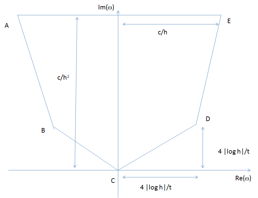
Figure 1. Contour of integration for the integral in (11.9). ${\mathcal{C}}_{+}$ is the countour joining the point $D$ to the points $E,A,B$. ${\mathcal{C}}_{-}$ is the countour joining the point $B$ to $C$ to $D$.

Let us introduce the following Green’s function:

(11.8) $$G_{m}(x,y;\omega)=\int_{0}^{\infty}U_{m}(x,0;y,t)e^{-i\omega t}dt={1\over\mathcal{L}+i\omega}(x,y).$$

The propagator can be expressed as the following contour integral

(11.9) $$U_{m}(x,0;y,T)=\int_{{\mathcal{C}}_{-}}{d\omega\over 2\pi}G_{m}(x,y;\omega)e^{i\omega T}+\int_{{\mathcal{C}}_{+}}{d\omega\over 2\pi}G_{m}(x,y;\omega)e^{i\omega T}.$$

Here, ${\mathcal{C}}_{+}$ is the contour joining the point $D$ to the points $E,A,B$ in Fig. 1, while ${\mathcal{C}}_{-}$ is the contour joining the point $B$ to $C$ to $D$. By design, each point $\omega$ on the upper path ${\mathcal{C}}_{+}$ is separated from the spectrum of $\mathcal{L}$.

Lemma 1.

For $m$ sufficiently large, there is a constant $c>0$ such that

(11.10) $$\bigg{\lvert}\int_{{\mathcal{C}}_{+}}{d\omega\over 2\pi}G_{m}(x,y;\omega)e^{i\omega T}\bigg{\lvert}\leq ch^{3}.$$

Proof.

The proof is based on the geometric series expansion

(11.11) $$G_{m}(\omega)={1\over{\mathcal{L}}^{m}+i\omega}=\sum_{j=0}^{\infty}{1\over{1\over 2}\sigma^{2}\Delta^{m}+i\omega}\bigg{[}\mu\nabla^{m}{1\over{1\over 2}\sigma^{2}\Delta^{m}+i\omega}\bigg{]}^{j}$$

whose convergence for $\omega\in{\mathcal{C}}_{+}$ can be established by means of a Kato-Rellich relative bound, see [Ka1976]. More precisely, for any $\alpha>0$, one can find a $\beta>0$ such that the operators $\nabla^{m}$ and $\Delta^{m}$ satisfy the following relative bound estimate:

(11.12) $$\lvert\lvert\nabla^{m}f\lvert\lvert_{2}\leq\alpha\lvert\lvert\Delta^{m}f\lvert\lvert_{2}+\beta\lvert\lvert f\lvert\lvert_{2}.$$

for all periodic functions $f$ and all $m\geq m_{0}$. This bound can be derived by observing that $\nabla^{m}$ and $\Delta^{m}$ can be diagonalized simultaneously by a Fourier transform, as done in the previous section, and by observing that for any $\alpha>0$, one can find a $\beta>0$ such that

(11.13) $$\bigg{\lvert}{\sin h_{m}p\over h_{m}}\bigg{\lvert}\leq\alpha\bigg{\lvert}{\cos h_{m}p-1\over h_{m}^{2}}\bigg{\lvert}+\beta$$

for all $m\geq m_{0}$ and all $p\in B_{m}$.

Under the same conditions, we also have that

(11.14) $$\big{\lvert}\big{\lvert}\mu\nabla^{m}f\big{\lvert}\big{\lvert}_{2}\leq{2M\alpha\over\Sigma_{0}^{2}}\bigg{\lvert}\bigg{\lvert}{1\over 2}\sigma^{2}\Delta^{m}f\bigg{\lvert}\bigg{\lvert}_{2}+\beta\lvert\lvert f\lvert\lvert_{2}.$$

Hence

(11.15) $$\bigg{\lvert}\bigg{\lvert}\mu\nabla^{m}{1\over{1\over 2}\sigma^{2}\Delta^{m}+i\omega}f\bigg{\lvert}\bigg{\lvert}_{2}\leq{2M\alpha\over\Sigma_{0}^{2}}\bigg{\lvert}\bigg{\lvert}{1\over 2}\sigma^{2}\Delta^{m}{1\over{1\over 2}\sigma^{2}\Delta^{m}+i\omega}f\bigg{\lvert}\bigg{\lvert}_{2}+\beta\bigg{\lvert}\bigg{\lvert}{1\over{1\over 2}\sigma^{2}\Delta^{m}+i\omega}f\bigg{\lvert}\bigg{\lvert}_{2}<1$$

where the last inequality holds if $\omega\in{\mathcal{C}}_{+}$, if $\alpha$ is chosen sufficiently small and if $m$ is large enough. In this case, the geometric series expansion converges in (11.11) converges in $L^{2}$ operator norm. The uniform norm of the kernel $\lvert G_{m}(x,y;\omega)\lvert$ is pointwise bounded from above by $h_{m}^{-1}$.

Since the points $B$ and $D$ have imaginary part equal at height $4{\lvert\log h_{m}\lvert\over T}$, the integral over the contour ${\mathcal{C}}_{+}$ converges also and is bounded from above by $ch_{m}^{3}$ in uniform norm.

∎

Lemma 2.

If $q\geq{e^{2}\Sigma_{1}^{2}T\over 2h_{m}^{2}}$ we have that

(11.16) $$W_{m}(\gamma,q;0,T)\leq\sqrt{q\over 2\pi}\exp\left(-{\Sigma_{0}^{2}T\over 2}-q\right).$$

Proof.

Let us define the function

(11.17) $$\phi(t)={\Sigma_{1}^{2}\over 2h_{m}^{2}}\;e^{-{\Sigma_{0}^{2}t\over 2h_{m}^{2}}}\;1(t\geq 0)$$

where $1(t\geq 0)$ is the characteristic function of ${\mathbb{R}}_{+}$. We have that

(11.18) $$W_{m}(\gamma,q;0,T)\leq\phi^{\star q}(T)$$

where $\phi^{\star q}$ is the $q-$th convolution power, i.e. the $q-$fold convolution product of the function $\phi$ by itself. The Fourier transform of $\phi(t)$ is given by

(11.19) $$\hat{\phi}(\omega)={\Sigma_{1}^{2}\over 2h_{m}^{2}}\int_{0}^{\infty}e^{-i\omega t-{\Sigma_{0}^{2}t\over 2h_{m}^{2}}}dt={\Sigma_{1}^{2}\over 2i\omega h_{m}^{2}+\Sigma_{0}^{2}}.$$

The convolution power is given by the following inverse Fourier transform:

(11.20) $$\phi^{\star q}(T)=\int_{0}^{\infty}\hat{\phi}(\omega)^{q}e^{i\omega T}=\left({\Sigma_{1}\over\Sigma_{0}}\right)^{2q}\int_{-\infty}^{\infty}\left(1+{2i\omega h_{m}^{2}\over\Sigma_{0}^{2}}\right)^{-q}e^{i\omega T}{d\omega\over 2\pi}.$$

Introducing the new variable $z=1+{2i\omega h_{m}^{2}\over\Sigma_{0}^{2}}$, the integral can be recast as follows

(11.21) $$\phi^{\star q}(T)={\Sigma_{0}^{2-2q}\Sigma_{1}^{2q}\over 4\pi ih_{m}^{2}}\lim_{R\to\infty}\int_{{\mathcal{C}}_{R}}z^{-q}\exp\left({\Sigma_{0}^{2}T\over 2h_{m}^{2}}(z-1)\right)dz$$

where ${\mathcal{C}}_{R}$ is the contour in Fig. 2. Using the residue theorem and noticing that the only pole of the integrand is at $z=0$, we find

(11.22) $$\phi^{\star q}(T)={1\over(q-1)!}\left({\Sigma_{1}^{2}T\over 2h_{m}^{2}}\right)^{q}\exp\left(-\Sigma_{0}^{2}T\over 2h_{m}^{2}\right).$$

Making use of Stirling’s formula $q!\approx\sqrt{2\pi}q^{q+{1\over 2}}e^{-q}$, we find

(11.23) $$\phi^{\star q}(T)\approx\sqrt{q\over 2\pi}\exp\left(-{\Sigma_{0}^{2}T\over 2h_{m}^{2}}+q\log{\Sigma_{1}^{2}T\over 2h_{m}^{2}}+q(1-\log q)\right).$$

If $\log q\geq\log{\Sigma_{1}^{2}T\over 2h_{m}^{2}}+2$, then we arrive at the bound in (11.16).

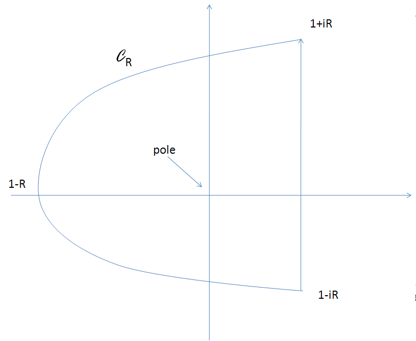
Figure 2. Contour of integration ${\mathcal{C}}_{R}$ for the integral in (11.21).

∎

Definition 41.

(Decorating Paths.) Let $m\geq m_{0}$ and let $\gamma=\{y_{0},y_{1},y_{2},....\}$ be a symbolic sequence in $\Gamma_{m}$. A decorating path around $\gamma$ is defined as a symbolic sequence $\gamma^{\prime}=\{y_{0},y_{1}^{\prime},y_{2}^{\prime},....\}$ with $y_{i}^{\prime}\in h_{m+1}{\mathbb{Z}}$ containing the sequence $\gamma$ as a subset and such that if $y_{j}^{\prime}=y_{i}$ and $y_{k}^{\prime}=y_{i+1}$, then all elements $y_{n}^{\prime}$ with $j<n<k$ are such that $\lvert y_{n}^{\prime}-y_{j}^{\prime}\lvert\leq h_{m+1}$. Let ${\mathcal{D}}_{m+1}(\gamma)$ be the set of all decorating sequences around $\gamma$. The decorated weights are defined as follows:

(11.24) $${\tilde{W}}_{m}(\gamma,q;0,T)=\sum_{q^{\prime}=q}^{\infty}\sum_{\begin{matrix}\gamma^{\prime}\in{\mathcal{D}}_{m+1}(\gamma)\\ \gamma^{\prime}_{q^{\prime}}=\gamma_{q}\end{matrix}}W_{m+1}(\gamma^{\prime},q^{\prime};0,T).$$

Finally, let us introduce also the following Fourier transform:

(11.25) $$\hat{W}_{m}(\gamma,q;\omega)=\int_{0}^{\infty}W_{m}(\gamma,q;0,t)e^{i\omega t}dt,\;\;\;\;\hat{\tilde{W}}_{m}(\gamma,q;\omega)=\int_{0}^{\infty}\tilde{W}_{m}(\gamma,q;0,t)e^{i\omega t}dt.$$

Definition 42.

(Notations.) In the following, we set $h=h_{m+1}$ so that $h_{m}=2h$. We also use the Landau notation $O(h^{n})$ to indicate a function $f(h)$ such that $h^{-n}f(h)$ is bounded in a neighborhood of $(0)$.

Lemma 3.

Let $x,y\in A_{m}$ and let ${\mathcal{C}_{-}}$ be an integration contour as in Fig. 1. Then

(11.26) $$\bigg{\lvert}\bigg{(}\int_{{\mathcal{C}}_{-}}2G_{m+1}(x,y;\omega)-G_{m}(x,y;\omega)\bigg{)}e^{i\omega T}{d\omega\over 2\pi}\bigg{\lvert}=O(h^{3}).$$

Proof.

We have that

(11.27) $$2G_{m+1}(x,y;\omega)-G_{m}(x,y;\omega)= \sum_{q=1}^{\infty}2^{-q}\sum_{\begin{matrix}\gamma\in\Gamma_{m}:\gamma_{0}=x,\gamma_{q}=y\\ \lvert\gamma_{j}-\gamma_{j-1}\lvert=1\forall j\geq 1\end{matrix}}\left(2\hat{\tilde{W}}_{m}(\gamma,q;\omega)-\hat{W}_{m}(\gamma,q;\omega)\right).$$

The number of paths over which the summation is extended is

(11.28) $$N(\gamma,q;x,y)\equiv\sharp\{\gamma\in\Gamma_{m}:\gamma_{0}=x,\gamma_{q}=y,\lvert\gamma_{j}-\gamma_{j-1}\lvert=1\forall j\geq 1\}=\left(\begin{matrix}q\\ {q\over 2}+k\end{matrix}\right)$$

where $k={\lvert y-x\lvert\over h_{m}}.$ Applying Stirling’s formula we find

(11.29) $$N_{\gamma}\lesssim 2^{q}\sqrt{2\over\pi q}.$$

Hence

$$\bigg{\lvert}\int_{{\mathcal{C}}_{-}}\bigg{(}2G_{m+1}(x,y;\omega)-G_{m}(x,y;\omega)\bigg{)}e^{i\omega T}{d\omega\over 2\pi}\bigg{\lvert}$$

$$\leq c\sum_{q=1}^{\infty}\sqrt{1\over q}\max_{\begin{matrix}\gamma\in\Gamma_{m}:\gamma_{0}=x,\gamma_{q}=y\\ \lvert\gamma_{j}-\gamma_{j-1}\lvert=1\forall j\geq 1\end{matrix}}\bigg{\lvert}\int_{{\mathcal{C}}_{-}}\bigg{(}2\hat{\tilde{W}}_{m}(\gamma,q;\omega)-\hat{W}_{m}(\gamma,q;\omega)\bigg{)}e^{i\omega T}{d\omega\over 2\pi}\bigg{\lvert}.$$

for some constant $c\approx\sqrt{2\over\pi}>0$. It suffices to extend the summation over $q$ only up to

(11.31) $$q_{\rm max}\equiv{e^{2}\Sigma_{1}^{2}T\over 2h^{2}}.$$

To resum beyond this threshold, one can use the previous lemma. More precisely, we have that

$$\bigg{\lvert}\int_{{\mathcal{C}}_{-}}\bigg{(}2G_{m+1}(x,y;\omega)-G_{m}(x,y;\omega)\bigg{)}e^{i\omega T}{d\omega\over 2\pi}\bigg{\lvert}$$

$$\leq c\sqrt{q_{\rm max}}\max_{\begin{matrix}q,\gamma\in\Gamma_{m}:\gamma_{0}=x,\gamma_{q}=y\\ \lvert\gamma_{j}-\gamma_{j-1}\lvert=1\forall j\geq 1\end{matrix}}\bigg{\lvert}\int_{{\mathcal{C}}_{-}}\bigg{(}2\hat{\tilde{W}}_{m}(\gamma,q;\omega)-\hat{W}_{m}(\gamma,q;\omega)\bigg{)}e^{i\omega T}{d\omega\over 2\pi}\bigg{\lvert}.$$

Let $v(x)=\sigma(x)^{2}$. To evaluate the resummed weight function, let us form the matrix

(11.33) $$\bar{\mathcal{L}}(x;h)=\left(\begin{matrix}-{v\left(x+h\right)\over h^{2}}&&{v\left(x+h\right)\over 2h^{2}}-{\mu(x+h)\over 2h}&&0\\ {v\left(x\right)\over 2h^{2}}+\mu(x)/(2h)&&-{v\left(x\right)\over h^{2}}&&{v\left(x\right)\over 2h^{2}}-{\mu(x)\over 2h}\\ 0&&{v\left(x-h\right)\over 2h^{2}}+{\mu(x-h)\over 2h}&&-{v\left(x-h\right)\over h^{2}}\end{matrix}\right)$$

and decompose it as follows:

(11.34) $$\bar{\mathcal{L}}(x;h)={1\over h^{2}}\bar{\mathcal{L}}_{0}(x)+{1\over h}\bar{\mathcal{L}}_{1}(x)+\bar{\mathcal{L}}_{2}(x)+h\bar{\mathcal{L}}_{3}(x)+O(h^{2}).$$

where

(11.35) $$\bar{\mathcal{L}}_{0}(x)=\left(\begin{matrix}-v(x)&&{1\over 2}{v(x)}&&0\\ {1\over 2}{v(x)}&&-{v(x)}&&{1\over 2}{v(x)}\\ 0&&{1\over 2}{v(x)}&&-{v(x)}\end{matrix}\right),$$

(11.36) $$\bar{\mathcal{L}}_{1}(x)=\left(\begin{matrix}-v^{\prime}(x)&&{1\over 2}v^{\prime}(x)-{1\over 2}\mu(x)&&0\\ {1\over 2}\mu(x)&&0&&-{1\over 2}\mu(x)\\ 0&&-{1\over 2}v^{\prime}(x)+{1\over 2}\mu(x)&&v^{\prime}(x)\end{matrix}\right),$$

(11.37) $$\bar{\mathcal{L}}_{2}(x)=\left(\begin{matrix}-{1\over 2}v^{\prime\prime}(x)&&{1\over 4}v^{\prime\prime}(x)-{1\over 2}\mu^{\prime}(x)&&0\\ 0&&0&&0\\ 0&&{1\over 4}v^{\prime\prime}(x)-{1\over 2}\mu^{\prime}(x)&&-{1\over 2}v^{\prime\prime}(x)\end{matrix}\right).$$

and

(11.38) $$\bar{\mathcal{L}}_{3}(x)=\left(\begin{matrix}-{1\over 6}v^{\prime\prime\prime}(x)&&{1\over 12}v^{\prime\prime\prime}(x)-{1\over 4}\mu^{\prime\prime}(x)&&0\\ 0&&0&&0\\ 0&&-{1\over 12}v^{\prime\prime\prime}(x)+{1\over 4}\mu^{\prime\prime}(x)&&{1\over 6}v^{\prime\prime\prime}(x)\end{matrix}\right).$$

Let us introduce the sign variable $\tau=\pm 1$, the functions

(11.39) $$\phi_{0}(t,x,\tau) \equiv 2{\mathcal{L}}_{m}(x,x+2\tau h)e^{t{\mathcal{L}}_{m}(x,x)}1(t\geq 0)$$

(11.40) $$\phi_{1}(t,x,\tau) \equiv 2{\mathcal{L}}_{m+1}(x+\tau h,x+2\tau h)e^{t\bar{\mathcal{L}}(x;h)}(x,x+\tau h)1(t\geq 0)$$

and their Fourier transforms

$$\hat{\phi}_{0}(\omega,x,\tau) =\left({v(x)\over 4h^{2}}+\tau{\mu(x)\over 2h}\right)\left({v(x)\over 4h^{2}}+i\omega\right)^{-1}$$

$$\hat{\phi}_{1}(\omega,x,\tau) =\left({v(x)\over h^{2}}+\tau{\mu(x)+v^{\prime}(x)\over h}+{v^{\prime\prime}(x)+\mu^{\prime}(x)\over 2}+\left({v^{\prime\prime\prime}(x)\over 6}+{\mu^{\prime\prime}(x)\over 2}\right)\tau h+O(h^{2})\right)$$

(11.41) $$\hskip 227.62204pt<x\lvert\left(-\bar{\mathcal{L}}(x;h)+i\omega\right)^{-1}\lvert x+\tau h>.$$

where

(11.42) $$\lvert x>=\left(\begin{matrix}0\\ 1\\ 0\end{matrix}\right),\;\;\;\;{\rm and}\;\;\;\;\lvert x+\tau h>=\left(\begin{matrix}\delta_{\tau,1}\\ 0\\ \delta_{\tau,-1}\end{matrix}\right).$$

We also require the functions

(11.43) $$\psi_{0}(t,x)\equiv e^{t{\mathcal{L}}_{m}(x,x)}1(t\geq 0),\;\;\;\;\;\;\psi_{1}(t,x)\equiv e^{t\bar{\mathcal{L}}(y;h)}(x,x)1(t\geq 0)$$

and the corresponding Fourier transforms

(11.44) $$\hat{\psi}_{0}(\omega,x)=\left({v(x)\over 4h^{2}}+i\omega\right)^{-1},\;\;\;\;\;\hat{\psi}_{1}(\omega,x)=<x\lvert\left(-\bar{\mathcal{L}}(x;h)+i\omega\right)^{-1}\lvert x>.$$

If $\gamma$ is a symbolic sequence, then

(11.45) $$\hat{W}_{m}(\gamma,q;\omega) =\hat{\psi}_{0}(\omega,\gamma_{q})\prod_{j=0}^{q-1}\hat{\phi}_{0}(\omega;\gamma_{j},{\rm sgn}(\gamma_{j+1}-\gamma_{j}))$$

(11.46) $$\hat{\tilde{W}}_{m}(\gamma,q;\omega) =\hat{\psi}_{1}(\omega,\gamma_{q})\prod_{j=0}^{q-1}\hat{\phi}_{1}(\omega;\gamma_{j},{\rm sgn}(\gamma_{j+1}-\gamma_{j})).$$

Let us estimate the difference between the functions $\hat{\phi}_{1}(\omega,x,\tau)$ and $\hat{\phi}_{2}(\omega,x,\tau)$ assuming that $\omega$ is in the contour ${\mathcal{C}}_{-}$ in Fig. 2. Retaining only terms up to order up to $O(h^{3})$, we find

$$\hat{\phi}_{0}(\omega,x,\tau)=1+{2\mu(x)\tau h\over v(x)}-{4i\omega h^{2}\over v(x)}-8\mu(x){i\omega\tau h^{3}\over v(x)^{2}}-{16\omega^{2}h^{4}\over v(x)^{2}}+O(h^{5}).$$

A lengthy but straightforward calculation which is best carried out using a symbolic manipulation program, gives

$$\hat{\phi}_{1}(\omega,x,\tau)=1+{2\mu(x)\tau h\over v(x)}-{4i\omega h^{2}\over v(x)}-\big{[}8\mu(x)-v^{\prime}(x)\big{]}{i\omega\tau h^{3}\over v(x)^{2}}$$

$$\hskip 170.71652pt+r(x)\cdot h^{3}\tau+i\omega h^{4}p(x)-{14\omega^{2}h^{4}\over v(x)^{2}}+O(h^{5})$$

where

$$r(x)={1\over 2v(x)^{3}}\big{[}\mu^{\prime\prime}(x)v(x)-4\mu(x)^{3}+2v^{\prime}(x)\mu(x)^{2}-2v^{\prime}(x)v(x)\mu^{\prime}(x)$$

$$\hskip 170.71652pt-\big{(}2\mu(x)\mu^{\prime}(x)+v^{\prime\prime}(x)v(x)-2v^{\prime}(x)^{2}\big{)}\mu(x)\big{]}.$$

$$p(x)={1\over v(x)^{3}}\big{[}4\mu(x)^{2}-2v^{\prime}(x)\mu(x)+4v(x)\mu^{\prime}(x)+v^{\prime\prime}(x)v(x)-2v^{\prime}(x)^{2}\big{]}.$$

We have that

$$\sum_{j=0}^{q-1}\bigg{(}\log\hat{\phi}_{0}(\omega;\gamma_{j},{\rm sgn}(\gamma_{j+1}-\gamma_{j}))-\log\hat{\phi}_{1}(\omega;\gamma_{j},{\rm sgn}(\gamma_{j+1}-\gamma_{j}))\bigg{)}$$

$$=\sum_{j=0}^{q-1}\bigg{(}{i\omega v^{\prime}(\gamma_{j})\over v(\gamma_{j})^{2}}+r(\gamma_{j})\bigg{)}h^{3}{\rm sgn}(\gamma_{j+1}-\gamma_{j})+\big{(}\lvert\omega\lvert\lvert\lvert p\lvert\lvert_{\infty}+2\lvert\omega\lvert^{2}\lvert\lvert v^{-2}\lvert\lvert_{\infty}\big{)}O(h^{4}q)$$

$$=i\omega h^{2}\log\bigg{(}{v(\gamma_{q})\over v(\gamma_{0})}\bigg{)}+h^{2}\big{(}R(\gamma_{q})-R(\gamma_{0})\big{)}+\big{(}\lvert\omega\lvert\lvert\lvert p\lvert\lvert_{\infty}+2\lvert\omega\lvert^{2}\lvert\lvert v^{-2}\lvert\lvert_{\infty}\big{)}O(h^{4}q)$$

where $R(x)$ is a primitive of $r(x)$, i.e.

(11.51) $$R(x)=\int^{x}r(z)dz.$$

We conclude that there is a constant $c>0$ such that

(11.52) $$\bigg{\lvert}\int_{{\mathcal{C}}_{-}}\bigg{(}\prod_{j=0}^{q-1}\hat{\phi}_{0}(\omega;\gamma_{j},{\rm sgn}(\gamma_{j+1}-\gamma_{j}))-\prod_{j=0}^{q-1}\hat{\phi}_{1}(\omega;\gamma_{j},{\rm sgn}(\gamma_{j+1}-\gamma_{j}))\bigg{)}e^{i\omega T}{d\omega\over 2\pi}\bigg{\lvert}\leq ch^{2}.$$

for all $q\leq q_{\max}$. Here we use the decay of $e^{i\omega T}$ in the upper half of the complex $\omega$ plane to offset the $\omega$ dependencies in the integrand. Similar calculations lead to the following expansions:

(11.53) $$\hat{\psi}_{0}(\omega,y)={4h^{2}\over v(y)}+O(\omega h^{4}),\;\;\;\;\;\hat{\psi}_{1}(\omega,y)={2h^{2}\over v(y)}+O(\omega h^{4})={1\over 2}\hat{\psi}_{0}(\omega,y)+O(\omega h^{4}).$$

Since $q<ch^{-2}$ and $\omega\leq\lvert\log h\lvert$, we find

(11.54) $$\bigg{\lvert}\int_{{\mathcal{C}}_{-}}\bigg{(}2G_{m+1}(x,y;\omega)-G_{m}(x,y;\omega)\bigg{)}e^{i\omega T}{d\omega\over 2\pi}\bigg{\lvert}\leq c{q_{\rm max}}^{1\over 2}h^{4}\leq ch^{3}.$$

This completes the proof of the Lemma and of the Theorem. ∎

12. Convergence of Time Discretization Schemes

In this section we analyze the convergence of the time discretized kernel that is obtained by means of fast exponentiation.

Let $A=(A_{m}),m=m_{0},m_{0}+1,...$ be a simplicial sequence converging to an interval $\lim_{m\to\infty}A_{m}=[0,L]\subset{\mathbb{R}}$, where $0<L<\infty$. Let $\mu(x)$ and $\sigma(x)$ be functions on $[0,L]$ satisfying all the conditions in the previous section and consider the generator of a diffusion on $A_{m}$ of the form

(12.1) $${\mathcal{L}}_{m}=\mu(x)\nabla_{h_{m}}+{1\over 2}\sigma(x)^{2}\Delta_{h_{m}}.$$

Theorem 18.

(Convergence Estimates for Fast Exponentiation.) Let $\delta t>0$ and consider the discretized kernel

(12.2) $$U^{\delta t}_{m}(x,0;y,T)=\left(1+\delta t{\mathcal{L}}_{m}\right)^{T\over\delta t}(x,0;y,T).$$

where ${\mathcal{L}}_{m}$ is the operator in (12.1) and $\delta t_{m}$ is so small that

(12.3) $$\min_{x\in A_{m}}1+\delta t_{m}{\mathcal{L}}_{m}(x,x)>0$$

Assume that boundary conditions are either periodic or absorbing and that the ratio ${T\over\delta t}=N$ is an integer. Then there is a constant $c>0$ such that

(12.4) $$\lvert h_{m}^{-1}U_{m}(x,0;y,T)-h_{m}^{-1}U_{m}^{\delta t}(x,0;y,T)\lvert\leq ch_{m}^{2}$$

for all $m\geq m_{0}$ and all $y\in A_{m}$.

Proof.

A Dyson expansion can also be obtained for the time-discretized kernel and has the form

$$U_{m}^{\delta t}(y_{1},0;y_{2},T)= \sum_{q=1}^{\infty}\sum_{\gamma\in\Gamma_{m}:\gamma_{0}=x,\gamma_{q}=y}\sum_{k_{1}=1}^{N}\sum_{k_{2}=k_{1}+1}^{N}...\sum_{k_{q}=k_{q-1}+1}^{N}$$

(12.5) $$\bigg{(}1+\delta t{\mathcal{L}}_{m}(\gamma_{0},\gamma_{0})\bigg{)}^{k_{1}-1}(\delta t)^{q}\prod_{j=1}^{q}{\mathcal{L}}_{m}(\gamma_{j-1},\gamma_{j})\bigg{(}1+\delta t{\mathcal{L}}_{m}(\gamma_{j},\gamma_{j})\bigg{)}^{k_{j+1}-k_{j}-1}$$

where $t_{q+1}=T$ and $k_{q+1}=N$. In this case, the propagator can be expressed through a Fourier integral as follows:

(12.6) $$U_{m}^{\delta t}(y_{1},0;y_{2},T)=\int_{-{\pi\over\delta t}}^{\pi\over\delta t}G_{m}^{\delta t}(y_{1},y_{2};\omega)e^{i\omega t}{d\omega\over 2\pi}$$

where

(12.7) $$G_{m}^{\delta t}(y_{1},y_{2};\omega)=\delta t\sum_{j=0}^{T\over\delta t}U_{m}^{\delta t}(y_{1},0;y_{2},j\delta t)e^{-i\omega j\delta t}.$$

The propagator can also be represented as the limit

(12.8) $$U_{m}^{\delta t}(y_{1},0;y_{2},T)=\lim_{H\to\infty}\int_{{\mathcal{C}}_{H}}G_{m}^{\delta t}(y_{1},y_{2};\omega)e^{i\omega t}{d\omega\over 2\pi}$$

where ${\mathcal{C}}_{H}$ is the contour in Fig. 3. This is due to the fact that the integral along the segments $BC$ and $DA$ are the negative of each other, while the integral over $CD$ tends to zero exponentially fast as $\Im(\omega)\to\infty$, where $\Im(\omega)$ is the imaginary part of $\omega$. Using Cauchy’s theorem, the contour in Fig. 3 can be deformed into the contour in Fig. 1. To estimate the discrepancy between the time-discretized kernel and the continuous time one, one can thus compare the Green’s function along such contour. Again, the only arc that requires detailed attention is the arc $BCD$, as the integral over rest of the contour of integration can be bounded from above as in the previous section.

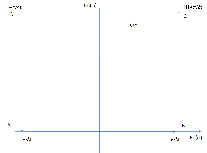
Figure 3. Contour of integration for the integral in (12.8).

Let $h=h_{m}$ and let us introduce the two functions

(12.9) $$\phi_{0}(t,x,\tau) \equiv 2{\mathcal{L}}_{m}(x,x+\tau h)e^{t{\mathcal{L}}_{m}(x,x)}1(t\geq 0),$$

(12.10) $$\phi_{\delta t}(j,x,\tau) \equiv 2{\mathcal{L}}_{m}(x,x+\tau h)\big{(}1+\delta t{\mathcal{L}}_{m}(x,x)\big{)}^{j-1}.$$

and the corresponding Fourier transforms

(12.11) $$\hat{\phi}_{0}(\omega,x,\tau) =\int_{0}^{\infty}\phi_{0}(t,x,\tau)e^{-i\omega t}{d\omega\over 2\pi}=\left({v(x)\over h^{2}}+\tau{\mu(x)\over h}\right)\left({v(x)\over h^{2}}+i\omega\right)^{-1}$$

(12.12) $$\hat{\phi}_{\delta t}(\omega,x,\tau) =\sum_{j=0}^{t\over\delta t}\phi_{\delta t}(j,x,\tau)e^{-i\omega j\delta t}=\left({v(x)\over h^{2}}+\tau{\mu(x)\over h}\right)\left(e^{i\omega\delta t}-1+\delta t{v(x)\over h^{2}}\right)^{-1}.$$

We have that

$$\hat{\phi}_{\delta t}(\omega,x,\tau) =\left({v(x)\over h^{2}}+\tau{\mu(x)\over h}\right)\left(i\omega+{v(x)\over h^{2}}-{\omega^{2}\over 2}\delta t+O(\delta t^{2})\right)^{-1}$$

(12.13) $$=\hat{\phi}_{0}(\omega,x,\tau)+{\omega^{2}\over 2v(x)}h^{2}\delta t+O(h^{2}\delta t^{2}).=\hat{\phi}_{0}(\omega,x,\tau)+O(h^{4}),$$

where the last step uses the fact that $\delta t=O(h^{2})$.

Let us also introduce the functions

(12.14) $$\psi_{0}(t,x,\tau) \equiv e^{t{\mathcal{L}}_{m}(x,x)}1(t\geq 0),\hskip 28.45274pt\psi_{\delta t}(j,x,\tau)\equiv\sum_{k=1}^{j}\big{(}1+\delta t{\mathcal{L}}_{m}(x,x)\big{)}^{j-1}.$$

and the corresponding Fourier transforms

(12.15) $$\hat{\psi}_{0}(\omega,x,\tau) =\left({v(x)\over h^{2}}+i\omega\right)^{-1},\hskip 28.45274pt\hat{\psi}_{\delta t}(\omega,x,\tau)=\left(e^{i\omega\delta t}-1+\delta t{v(x)\over h^{2}}\right)^{-1}.$$

Again we find that

(12.16) $$\hat{\psi}_{0}(\omega,x,\tau)=\hat{\psi}_{\delta t}(\omega,x,\tau)+O(h^{4}).$$

If $\gamma$ is a symbolic sequence, then let us set

(12.17) $$\hat{W}_{m}(\gamma,q;\omega) =\hat{\psi}_{0}(\omega,\gamma_{q})\prod_{j=0}^{q-1}\hat{\phi}_{0}(\omega;\gamma_{j},{\rm sgn}(\gamma_{j+1}-\gamma_{j}))$$

(12.18) $$\hat{W}_{m}^{\delta t}(\gamma,q;\omega) =\hat{\psi}_{\delta t}(\omega,\gamma_{q})\prod_{j=0}^{q-1}\hat{\phi}_{\delta t}(\omega;\gamma_{j},{\rm sgn}(\gamma_{j+1}-\gamma_{j})).$$

We have that

(12.19) $$G^{\delta t}_{m}(x,y;\omega)-G_{m}(x,y;\omega)= \sum_{q=1}^{\infty}2^{-q}\sum_{\begin{matrix}\gamma\in\Gamma_{m}:\gamma_{0}=x,\gamma_{q}=y\\ \lvert\gamma_{j}-\gamma_{j-1}\lvert=1\forall j\geq 1\end{matrix}}\left(\hat{W}_{m}^{\delta t}(\gamma,q;\omega)-\hat{W}_{m}(\gamma,q;\omega)\right).$$

The integration over the contour in Fig. 1 can again be split into an integration over the countour ${\mathcal{C}}_{-}$ and an integration over ${\mathcal{C}}_{+}$. The integral over ${\mathcal{C}}_{+}$ can be bounded from above thanks to Lemma 3. Furthermore, we have that

$$\bigg{\lvert}\int_{{\mathcal{C}}_{-}}\bigg{(}G^{\delta t}_{m}(x,y;\omega)-G_{m}(x,y;\omega)\bigg{)}e^{i\omega T}{d\omega\over 2\pi}\bigg{\lvert}$$

$$\leq c\sqrt{q_{\rm max}}\max_{\begin{matrix}q,\gamma\in\Gamma_{m}:\gamma_{0}=x,\gamma_{q}=y\\ \lvert\gamma_{j}-\gamma_{j-1}\lvert=1\forall j\geq 1\end{matrix}}\bigg{\lvert}\int_{{\mathcal{C}}_{-}}\bigg{(}\hat{W}_{m}^{\delta t}(\gamma,q;\omega)-\hat{W}_{m}(\gamma,q;\omega)\bigg{)}e^{i\omega T}{d\omega\over 2\pi}\bigg{\lvert}.$$

(12.20) $$\leq ch^{3}$$

∎

13. Hypergeometric Brownian Motion

This section is based on work in collaboration with Joe Campolieti, Peter Carr and Alex Lipton, see [ACCL2002].

In this section we pose the problem of constructing driftless diffusion models which reduce to a given diffusion by means of a combination of a measure change and a coordinate transformation.

Consider a Markov process on the simplicial sequence $A_{m}\subset{\mathbb{R}}^{d}$ with generator ${\mathcal{L}}_{m}(x,x^{\prime};t)$. Let $\rho$ be a real valued parameter and suppose $f_{m}^{1}(x)$ and $f_{m}^{2}(x)$ are two linearly independent solutions of the equation

(13.1) $$\sum_{x^{\prime}\in A_{m}}{\mathcal{L}}_{m}(x,x^{\prime};t)f_{m})(x^{\prime})=\rho f_{m}(x)$$

for all $x\in Int(A_{m})$. Notice that on the boundary $\partial(A_{m})$ these equations may fail and, in actual applications, they will indeed as a rule fail. Consider the function

(13.2) $$g_{m}(x;t)=e^{-\rho t}\big{(}c_{1}f_{m}^{1}(x)+c_{2}f_{m}^{2}(x)\big{)}$$

for some choice of constants $c_{1},c_{2}$ such that this function is strictly positive. This function satisfies the equation

(13.3) $${\partial g_{m}(x;t)\over\partial t}+({\mathcal{L}}_{m}g_{m})(x;t)=0.$$

Hence $g_{m}(x;t)$ defines a measure change and one can construct a new Markov generator by setting

(13.4) $${\mathcal{L}}_{m}^{g}(x,x^{\prime};t)={g_{m}(x^{\prime};t)\over g_{m}(x;t)}{\mathcal{L}}_{m}(x,x^{\prime};t)+{1\over g_{m}(x;t)}{\partial g_{m}(x;t)\over\partial t}\delta_{xx^{\prime}}.$$

Consider the linear fractional transformation

(13.5) $$Y_{m}(x)={c_{3}f_{m}^{1}(x)+c_{4}f_{m}^{2}(x)\over c_{1}f_{m}^{1}(x)+c_{2}f_{m}^{2}(x)}.$$

for some choice of constants $c_{3},c_{4}$.

Theorem 19.

(Linear Fractional Transformations.) The process $Y(x_{t})$ satisfies the martingale condition

(13.6) $$\lim_{s\downarrow 0}{1\over s}E_{t}\bigg{[}{Y_{m}(x_{t+s})-Y_{m}(x_{t})\over s}\bigg{]}=0.$$

for all $x_{t}\in Int(A_{m})$.

Proof.

We have that

$$\hskip-113.81102pt\lim_{s\downarrow 0}{1\over s}E_{t}\bigg{[}{Y_{m}(x_{t+s})-Y_{m}(x_{t})\over s}\bigg{]}=\sum_{x^{\prime}\in A_{m}}{\mathcal{L}}_{m}^{g}(x,x^{\prime})\big{(}Y_{m}(x^{\prime})-Y_{m}(x)\big{)}$$

$$={1\over g_{m}(x,t)}\bigg{(}\sum_{x^{\prime}\in A_{m}}{\mathcal{L}}_{m}(x,x^{\prime})\big{(}c_{3}f_{m}^{1}(x^{\prime})+c_{4}f_{m}^{2}(x^{\prime})\big{)}\bigg{)}+{1\over g_{m}(x,t)^{2}}{\partial g_{m}(x;t)\over\partial t}\big{(}c_{3}f_{m}^{1}(x)+c_{4}f_{m}^{2}(x)\big{)}$$

$$\hskip-248.96161pt=e^{\rho t}{\partial\over\partial t}\bigg{[}{e^{-\rho t}(c_{3}f_{m}^{1}(x)+c_{4}f_{m}^{2}(x))\over g_{m}(x,t)}\bigg{]}=0$$

∎

This Theorem provides a general methodology for constructing a process which is nearly a martingale out of a Markov process. In the particular case of one-dimensional diffusion processes, the construction gives rise to families with up to 7 adjustable parameters of analytically solvable diffusions with drift equal to zero within the interior of the domain of definition. What makes the case of one-dimensional diffusions special is the fact that the function $Y_{m}(x)$ is invertible in the limit as $m\to\infty$, i.e. either monotone increasing or monotone decreasing in this limit.

More specifically, consider the diffusion with Markov generator:

(13.8) $${\mathcal{L}}_{m}=\delta(x)\nabla_{h_{m}}+{1\over 2}\nu(x)^{2}\Delta_{h_{m}}.$$

where $x\in{\mathbb{R}}$. Two important cases are the CIR process (reducing to the Bessel equation in the continuous limit) for which

(13.9) $$\delta(x)=(\lambda_{0}+\lambda_{1}x),\;\;\;\;\;\nu(x)=\nu_{0}\sqrt{x}$$

with $x\in{\mathbb{R}}_{+}$ and the Jacobi process (reducing to a gaussian hypergeometric polynamials of type ${}_{2}F_{1}$) for which

(13.10) $$\delta(x)=(\lambda_{0}+\lambda_{1}x),\;\;\;\;\;\nu(x)=\nu_{0}\sqrt{x(1-x)}$$

and $x\in[0,1]$.

The construction above admits a continuous limit if the simplicial functions $f_{m}^{j}(x),j=1,2,3,4$ converge to twice differentiable functions $f^{j}(x),j=1,2,3,4$ and satisfy the equation

(13.11) $${\mathcal{L}}f=\rho f$$

within the interior of the domain $A=\lim_{m\to\infty}A_{m}$. Here

(13.12) $${\mathcal{L}}=\delta(x){\partial\over\partial x}+{1\over 2}\nu(x)^{2}{\partial^{2}\over\partial x^{2}}.$$

Theorem 20.

(Invertibility.) Let $f^{j}(x),j=1,2,3,4$ be functions satisfying equation 13.12 in the interior of the corresponding domain of definition and let

(13.13) $$Y(x)={c_{3}f^{1}(x)+c_{4}f^{2}(x)\over c_{1}f^{1}(x)+c_{2}f^{2}(x)}.$$

for some choice of constants $c_{1},c_{2},c_{3},c_{4}$ such that the denominator in this equation has no zeros. Then we have that

(13.14) $$Y(x)=\int^{x}{W(y)\over g(y)^{2}}dy+{\rm const}$$

where

(13.15) $$W(x)=\pm{\rm\sigma_{0}}\exp\bigg{(}-\int^{x}{2\delta(y)\over\nu(y)^{2}}dy\bigg{)}$$

where either sign would be allowed and $\sigma_{0}$ is a positive constant. In particular, the function $Y(x)$ is invertible.

Proof.

Let us introduce the Wronskian

(13.16) $$W(x)={dh(x)\over dx}g(x)-{dg(x)\over dx}h(x)$$

such that

(13.17) $$g(x)=c_{1}f^{1}(x)+c_{2}f^{2}(x),\;\;\;\;\;h(x)=c_{3}f^{1}(x)+c_{4}f^{2}(x).$$

A direct calculation shows that

(13.18) $${d\over dx}Y(x)=W(x)Y(x)$$

and

(13.19) $${d\over dx}W(x)=-{2\delta(x)\over\nu(x)^{2}}W(x).$$

Hence, (13.15) gives the solution to the equation in (13.19). ∎

Let $X(y)$ be the inverse of the function $Y(x)$, we have that

(13.20) $${dy\over\sigma(y)}=\pm{dX(y)\over\nu(X(y))}$$

where

(13.21) $$\sigma(y)=Y^{\prime}(X(y))\nu(X(y))={\sigma_{0}\nu(X(y))\exp\left({-2\int^{X(y)}{\delta(s)ds\over\nu(s)^{2}}}\right)\over g(X(y),\rho)^{2}}$$

Theorem 21.

(Kernel mapping.) In the limit $m\to\infty$, the propagator density for the process $Y_{t}$ with zero drift and volatility as in (13.21) is given by

(13.22) $$U(y_{0},0;y,t)={\nu(X(y))\over\sigma(y)}{g(X(y),\rho)\over g(X(y_{0}),\rho)}e^{-\rho t}u(X(y_{0}),0;X(y),t)$$

where $u(x_{0},0;x,t)$ is the propagator density for the process of generator (13.12).

Let us consider in detail the case of the CIR model in (13.9). If $\lambda_{1}=0$, then the pricing kernel for the state variable is expressed in terms of modified Bessel functions as follows:

(13.23) $$u(x,t;x_{0},0)=\left({x\over x_{0}}\right)^{{1\over 2}({2\lambda_{0}\over\nu_{0}^{2}}-1)}{e^{-2(x+x_{0})/\nu_{0}^{2}t}\over\nu_{0}^{2}t/2}I_{{2\lambda_{0}\over\nu_{0}^{2}}-1}\left({4\sqrt{xx_{0}}\over\nu_{0}^{2}t}\right)\,.$$

The generating function is

(13.24) $$\hat{v}(x,\rho)=x^{{1\over 2}(1-{2\lambda_{0}\over\nu_{0}^{2}})}\bigg{[}q_{1}I_{{2\lambda_{0}\over\nu_{0}^{2}}-1}\left(\sqrt{8\rho x\over\nu_{0}^{2}}\right)+q_{2}K_{{2\lambda_{0}\over\nu_{0}^{2}}-1}\left(\sqrt{8\rho x\over\nu_{0}^{2}}\right)\bigg{]}\,,$$

with arbitrary constants $q_{1}$,$q_{2}$. Here $I_{\nu}(z)$ is the modified Bessel function of order $\nu$ and $K_{\nu}(z)$ is the associated McDonalds function. In this case we obtain a dual family with 6 adjustable parameters.

In case $\lambda_{1}<0$. the propagator density for the state variable $x$ can still be expressed in terms of modified Bessel functions as follows:

(13.25) $$u(x,t;x_{0},0)=c_{t}\bigg{(}{xe^{-\lambda_{1}t}\over x_{0}}\bigg{)}^{{1\over 2}({2\lambda_{0}\over\nu_{0}^{2}}-1)}\exp\left[-c_{t}(x_{0}e^{\lambda_{1}t}+x)\right]I_{{2\lambda_{0}\over\nu_{0}^{2}}-1}\bigg{(}2c_{t}\sqrt{xx_{0}e^{\lambda_{1}t}}\bigg{)}\,,$$

where $c_{t}\equiv 2\lambda_{1}/(\nu_{0}^{2}(e^{\lambda_{1}t}-1))$. For a derivation see [Giorno88]. The general solution of equation (13.1) reduces to Whittaker’s equation and generating functions have the general form

(13.26) $$\hat{v}(x,\rho)=x^{-\lambda_{0}/\nu_{0}^{2}}e^{-\lambda_{1}x/\nu_{0}^{2}}\bigg{[}q_{1}W_{k,m}\bigg{(}-{2\lambda_{1}\over\nu_{0}^{2}}x\bigg{)}+q_{2}M_{k,m}\bigg{(}-{2\lambda_{1}\over\nu_{0}^{2}}x\bigg{)}\bigg{]}$$

for arbitrary constants $q_{1}$,$q_{2}$. Here $W_{k,m}(\cdot)$ and $M_{k,m}(\cdot)$ are Whittaker functions which can also be expressed in terms of confluent hypergeometric functions or in terms of Kummer functions.[Abramowitz] This construction gives rise to a dual family with 7 free parameters where

(13.27) $$k={\lambda_{0}\over\nu_{0}^{2}}+{\rho\over\lambda_{1}}\,,\,\,m={\lambda_{0}\over\nu_{0}^{2}}-{1\over 2}\,.$$

The 7 parameter family which reduces to the CIR model has a local volatility function defined on either an interval or on a half line and behaves asymptotically as the CEV volatility on one hand and as a quadratic model on the other. This hybrid shape allows for greater flexibility.

Next, we show that classic exact solutions in the literature, namely quadratic and CEV models, can all be rediscovered as particular cases of our general formula for the Bessel family where we make use of the above solutions to the underlying $x$ space process with $\beta={1\over 2}$, $\lambda_{1}=0$ and $\lambda\equiv\lambda_{0}$. Without loss of generality, we can fix $\nu_{0}=2$. Let’s specialize further to the case where

(13.28) $$Y(x)=\bar{y}-a{K_{{\lambda\over 2}-1}(\sqrt{2\rho x})\over I_{{\lambda\over 2}-1}(\sqrt{2\rho x})}$$

which leads to a transformed process $y_{t}=Y(x_{t})$ with volatility

(13.29) $$\sigma(y)={a\over\sqrt{X(y)}\big{[}I_{{\lambda\over 2}-1}(\sqrt{2\rho X(y)})\big{]}^{2}},$$

where $x=X(y)$ is the inverse of the function in equation (13.28). In this family, $a$ and $\rho$ are positive, $\bar{y}$ is arbitrary and $\lambda>2$. The function $Y(x)$ maps the half line $x\in[0,\infty)$ into $y\in(-\infty,\bar{y}]$, where $Y(x)$ is a strictly monotonically increasing function with $dY(x)/dx=\sigma(Y(x))/\nu(x)$. This solution region can be inverted so that $y\in[\bar{y},\infty)$. This is accomplished by either replacing $a$ by $-a$ in equation (13.28) or by applying a linear change of variables that maps $y$ into $2\bar{y}-y$. In this special case, we make use of the generating function in equation (13.24), with the choice $q_{2}=0$, and formula (13.22) reduces to

(13.30) $$U(y,t;y_{0},0)={e^{-\rho t-(X(y)+X(y_{0}))/2t}\over at}{X(y)\big{[}I_{{\lambda\over 2}-1}(\sqrt{2\rho X(y)})\big{]}^{3}\over I_{{\lambda\over 2}-1}(\sqrt{2\rho X(y_{0})})}I_{{\lambda\over 2}-1}\left({\sqrt{X(y)X(y_{0})}\over t}\right).$$

We note that this density integrates exactly to unity in $y$ space (i.e. no absorption).

Example 4.

(Quadratic volatility models) Pricing kernels for quadratic volatility models are readily obtained as a subset of the above general family with the special choice of parameter $\lambda=3$. After making the substitution $y\to 2\bar{y}-y$ and setting $a=(\bar{y}-\bar{\bar{y}})/\pi$ the transformation function $Y(x)$ becomes

(13.31) $$Y(x)=\bar{y}+{(\bar{y}-\bar{\bar{y}})\over\pi}{K_{1\over 2}(\sigma_{0}\sqrt{x}/2)\over I_{1\over 2}(\sigma_{0}\sqrt{x}/2)}=\bar{y}+{(\bar{y}-\bar{\bar{y}})\over\exp(\sigma_{0}\sqrt{x})-1}$$

where $\sigma_{0}>0$. Here, we assume that $\bar{y}>\bar{\bar{y}}$. The inverse transformation $X(y)$ is given by

(13.32) $$X(y)=(1/\sigma_{0}^{2})\log^{2}[1+(\bar{y}-\bar{\bar{y}})/(y-\bar{y})],$$

and the volatility function $\sigma(y)$ is obtained by insertion into equation (13.29) while using the Bessel function of order ${1\over 2}$,

(13.33) $$\sigma(y)={\sigma_{0}\over(\bar{y}-\bar{\bar{y}})}(y-\bar{y})(y-\bar{\bar{y}}).$$

Inserting the expression (13.32) into equation (13.30), one obtains the pricing kernel

(13.34) $$U(y,t;y_{0},0)={2e^{-\sigma_{0}^{2}t/8}\over\sigma(y)\sqrt{2\pi t}}\sqrt{(y_{0}-\bar{y})(y_{0}-\bar{\bar{y}})\over(y-\bar{y})(y-\bar{\bar{y}})}e^{-(\phi(y)^{2}+\phi(y_{0})^{2})/2\sigma_{0}^{2}t}\sinh\bigg{(}{\phi(y_{0})\phi(y)\over\sigma_{0}^{2}t}\bigg{)}$$

where $\phi(y)\equiv\log((y-\bar{\bar{y}})/(y-\bar{y}))$. In the special case of a volatility function with a double root, i.e.

(13.35) $$\sigma(y)=\sigma_{0}(y-\bar{y})^{2}$$

the pricing kernel is computed by taking the limit as $\bar{\bar{y}}\to\bar{y}$, and one finds

$$U(y,t;y_{0},0)={1\over\sigma_{0}\sqrt{2\pi t}}{(y_{0}-\bar{y})\over(y-\bar{y})^{3}}\bigg{[}e^{-\big{(}(y-\bar{y})^{-1}-(y_{0}-\bar{y})^{-1}\big{)}^{2}/2\sigma_{0}^{2}t}$$

(13.36) $$-e^{-\big{(}(y-\bar{y})^{-1}+(y_{0}-\bar{y})^{-1}\big{)}^{2}/2\sigma_{0}^{2}t}\bigg{]}.$$

Example 5.

(Lognormal models) The pricing kernel for the log-normal Black-Scholes model with $\sigma(y)=\sigma_{0}y$ is a particular case of the above formula for the quadratic model. The derivative with respect to $y$ of the quadratic volatility function in (13.33), evaluated at $y=\bar{y}$, is $\sigma_{0}$. Taking the limit $\bar{\bar{y}}\to-\infty$ (or $\bar{\bar{y}}<<\bar{y}$), while holding the other parameters fixed, one obtains $\sigma(y)=\sigma_{0}(y-\bar{y})$. The pricing kernel in (13.34) gives the kernel for the log-normal model in the limit $\bar{\bar{y}}\to-\infty$, i.e.

(13.37) $$U(y,t;y_{0},0)={1\over\ (y-\bar{y})\sigma_{0}\sqrt{2\pi t}}\exp\bigg{[}-\bigg{(}\log((y_{0}-\bar{y})/(y-\bar{y}))-{\sigma_{0}^{2}\over 2}t\bigg{)}^{2}\bigg{/}2\sigma_{0}^{2}t\bigg{]}.$$

Example 6.

(CEV model) The constant-elasticity-of-variance (CEV) model is recovered in the limiting case as $\rho\to 0$. Assume $\lambda>2$ and let $\theta>0$ be defined so that $\lambda=\theta^{-1}+2$. The transformation $y=Y(x)$

(13.38) $$Y(x)=\bar{y}+(\sigma_{0}^{2}x)^{-(2\theta)^{-1}}$$

has inverse $x=X(y)$ given by

(13.39) $$X(y)=\sigma_{0}^{-2}(y-\bar{y})^{-2\theta},$$

for any constant $\bar{y}$. The volatility function for this model is

(13.40) $$\sigma(y)={\sigma_{0}\over\lvert\theta\rvert}(y-\bar{y})^{1+\theta}.$$

In the limit $\rho\to 0$, the Laplace transform $\hat{v}(X(y),0)=1$, which implies that the numeraire change is trivial in this case. The pricing kernel can be evaluated by substitution into the general formula (13.22), and after collecting terms, it turns out to be

$$U(y,t;y_{0},0)={\lvert\theta\rvert\over\sigma_{0}^{2}t}{(y_{0}-\bar{y})^{1\over 2}\over(y-\bar{y})^{{3\over 2}+2\theta}}e^{-\big{(}(y-\bar{y})^{-2\theta}+(y_{0}-\bar{y})^{-2\theta}\big{)}/2\sigma_{0}^{2}t}$$

(13.41) $$I_{1\over 2\theta}\bigg{(}{\big{(}(y-\bar{y})(y_{0}-\bar{y})\big{)}^{-\theta}\over\sigma_{0}^{2}t}\bigg{)}.$$

This formula was derived in the case $\theta>0$, for which the limiting value $y=\bar{y}$ is not attained and the density is easily shown to integrate to unity (i.e. no absorption occurs and the density also vanishes at the endpoint $y=\bar{y}$). We note that the same formula solves the propagator equation for $\theta<0$, leading to the same Bessel equation of order $\pm(2\theta)^{-1}$. In the range $\theta<0$, however, the properties of the above pricing kernel are generally more subtle. In particular, one can show that the density integrates to unity for all values $\theta<-1/2$, hence no absorption occurs for $\theta\in(-\infty,-1/2)$. The boundary conditions for the density can be shown to be vanishing at $y=\bar{y}$ (i.e. paths do not attain the lower endpoint) for all $\theta<-1$. In contrast, for $\theta\in(-1,-1/2)$ the density becomes singular at the lower endpoint $y=\bar{y}$ (hence this corresponds to the case that the density has an integrable singularity for which paths can also attain the lower endpoint, but are not absorbed). For the special case of $\theta=-1/2$ the formula gives rise to absorption. [Note that only for the range $\theta\in(-1/2,0)$ the above pricing kernel is not useful since it gives rise to a density that has a non-integrable singularity at $y=\bar{y}$. In this case, however, another solution that is integrable is obtained by only replacing the order $(2\theta)^{-1}$ by $-(2\theta)^{-1}$ in the Bessel function. The latter solution for the density does not integrate to unity and hence gives rise to absorption which can be of use to price options in a credit setting.] The special case of $\theta=-1$ gives a nonzero constant value at the lower endpoint, and recovers the Wiener process with reflection and no absorption on the interval $[\bar{y},\infty)$ with

(13.42) $$U(y,t;y_{0},0)={1\over\sigma_{0}\sqrt{2\pi t}}\bigg{(}e^{-(y-y_{0})^{2}/2\sigma_{0}^{2}t}+e^{-(y+y_{0}-2\bar{y})^{2}/2\sigma_{0}^{2}t}\bigg{)}.$$

14. Stochastic Integrals for Diffusion Processes

This section provides a new derivation of a theorem by Cameron, Feynman, Girsanov, Ito, Kac and Martin, see [CameronMartin], [Ito1951], [Feynman1948] and [Kac1950]. This result is at the center of stochastic calculus and in the following sections, we derive far reaching extensions and applications.

Theorem 22.

(Cameron-Feynman-Girsanov-Ito-Kac-Martin.) Consider a diffusion process on the simplicial sequence $A_{m}\subset{\mathbb{R}}$ and of generator

(14.1) $${\mathcal{L}}_{m}=\mu(x,t)\nabla_{h_{m}}+{\sigma(x,t)^{2}\over 2}\Delta_{h_{m}}.$$

Consider also the process given by the integral

(14.2) $$I_{t}=\int_{0}^{t}a(x_{s},s)dx_{s}+b(x_{s},s)ds$$

where $a(x,t)$ and $b(x,t)$ are smooth functions in both arguments. Let us introduce also the function $\phi(x,t)=\int^{x}_{0}a(y,t)dy$. We have that

• Ito’s Lemma in integral form.

  (14.3) $$I_{t}=\phi(x_{t},t)-\phi(x_{0},0)+J_{t}+O(h).$$

  where

  (14.4) $$J_{t}=\int_{0}^{t}\bigg{(}b(x_{s},s)-{1\over 2}\sigma(x_{s},s)^{2}a^{\prime}(x_{s},s)-{\dot{\phi}}(x_{s},s)\bigg{)}ds.$$

  where $\dot{\phi}(x,t)={\partial\over\partial t}\phi(x,t)$ and $a^{\prime}(x,t)={\partial\over\partial x}a(x,t)$.

• Feynman-Kac formula. The characteristic function of $J_{t}$ on the bridge leading from $x$ to $y$ is given by

  (14.5) $$E_{0}\big{[}e^{ipJ_{t}}\delta(x_{t}=y)\lvert x_{0}=x\big{]}=P\exp\bigg{(}\int_{0}^{t}\bigg{(}{\mathcal{L}}(s)+ipb(s)-{ip\over 2}\sigma^{2}(s)a^{\prime}(s)-ip\dot{\phi}(s)+O(h)\bigg{)}\bigg{)}(x,y).$$

• Ito’s Lemma in differential form. Let $\phi(x,t)$ be a smooth function in both arguments. Then we have that

  $$\lim_{s\downarrow 0}E_{t}\left[s^{-1}(\phi(x_{t+s},t+s)-\phi(x_{t},t))\lvert x_{t}=x\right]$$

  (14.6) $$\hskip 85.35826pt={\partial\phi\over\partial t}(x,t)+\mu(x,t){\partial\phi\over\partial x}(x,t)+{\sigma(x,t)^{2}\over 2}{\partial^{2}\phi\over\partial x^{2}}(x,t)+O(h_{m})$$

  and

  (14.7) $$\lim_{s\downarrow 0}E_{t}\left[s^{-1}(\phi(x_{t+s},t+s)-\phi(x_{t},t))^{2}\lvert x_{t}=x\right]=\sigma(x,t)^{2}\left({\partial\phi\over\partial t}(x,t)\right)^{2}+O(h_{m}).$$

  For all $n\geq 3$ instead we have that

  (14.8) $$\lim_{h\downarrow 0}\lim_{s\downarrow 0}E_{t}\left[s^{-1}(\phi(x_{t+s},t+s)-\phi(x_{t},t))^{n}\lvert x_{t}=x\right]=0.$$

Proof.

Consider a discretization of the process $I_{t}=(\Delta I)n_{t}$. This can be accomplished by introducing a simplicial complex of one more dimension. Eventually in the proof, we shall take the limit as $\Delta I\to 0$ while leaving $h>0$ constant.

Consider the lifted generator

$$\tilde{\mathcal{L}}(x,n;x^{\prime},n^{\prime};t)=\left({\sigma(x)^{2}\over 2h^{2}}+{\mu(x,t)\over 2h}\right)\delta_{x^{\prime},x+h}\delta\bigg{(}n^{\prime}-n-\bigg{[}{a(x,t)h\over\Delta I}\bigg{]}\bigg{)}$$

$$+\left({\sigma(x,t)^{2}\over 2h^{2}}-{\mu(x,t)\over 2h}\right)\delta_{x^{\prime},x-h}\delta\bigg{(}n^{\prime}-n+\bigg{[}{a(x,t)h\over\Delta I}\bigg{]}\bigg{)}$$

(14.9) $$-{\sigma(x,t)^{2}\over h^{2}}\delta_{x^{\prime}x}\delta(n-n^{\prime})+{b(x,t)\over\Delta I}\big{(}\delta_{n^{\prime},n+1}-\delta_{n^{\prime}n}\big{)}$$

where $[a]$ stands for the nearest integer to $a$. The partial Fourier transform in the $n$ variable of this kernel is

$$\tilde{\mathcal{L}}_{p}(x,x^{\prime};t) = \sum_{n}\tilde{\mathcal{L}}(x,0;x^{\prime},n;t)e^{-i\Delta Ipn}$$

$$= \left({\sigma(x,t)^{2}\over 2h^{2}}+{\mu(x,t)\over 2h}\right)\exp\left(-i\left[{ha(x,t)\over\Delta I}\right]\Delta Ip\right)\delta_{x^{\prime},x+h}$$

$$+ \left({\sigma(x,t)^{2}\over 2h^{2}}-{\mu(x,t)\over 2h}\right)\exp\left(i\left[{ha(x,t)\over\Delta I}\right]\Delta Ip\right)\delta_{x^{\prime},x-h}$$

(14.10) $$- {\sigma(x,t)^{2}\over h^{2}}\delta_{x^{\prime}x}\delta(n-n^{\prime})+{b(x,t)\over\Delta I}\big{(}e^{ip\Delta I}-1\big{)}$$

In the limit as $\Delta I\to 0$ we find

$$\hskip-85.35826pt\tilde{\mathcal{L}}_{p}(x,x^{\prime};t)={\sigma(x,t)^{2}\over 2}\Delta_{h}+\left(\mu(x,t)-ip\sigma(x,t)^{2}a(x,t)\right)\nabla_{h}$$

(14.11) $$\hskip 85.35826pt-ipa(x,t)\mu(x,t)-{1\over 2}p^{2}\sigma(x,t)^{2}a(x,t)^{2}-ipb(x,t)+O(h).$$

Introducing the function $\phi(x,t)$ defined above, we find that

(14.12) $$e^{ip\phi(x,t)}{\mathcal{L}}(x,x^{\prime};t)e^{-ip\phi(x^{\prime},t)}=\tilde{\mathcal{L}}_{p}(x,x^{\prime};t)+ipb(x,t)\delta_{xx^{\prime}}-{ip\over 2}\sigma(x,t)^{2}a^{\prime}(x,t)\delta_{xx^{\prime}}+O(h).$$

This equality can be rearranged as follows:

(14.13) $$e^{-ip\phi(x,t)}\tilde{\mathcal{L}}(x,x^{\prime};t)e^{ip\phi(x^{\prime},t)}+ip\dot{\phi}(x,t)\delta_{xx^{\prime}}=$$

$$\hskip-113.81102pt{\mathcal{L}}_{p}(x,x^{\prime};t)-ipb(x,t)\delta_{xx^{\prime}}+{ip\over 2}\sigma(x,t)^{2}a^{\prime}(x,t)\delta_{xx^{\prime}}+ip\dot{\phi}(x,t)\delta_{xx^{\prime}}+O(h).$$

Hence

$$\hskip-284.52756ptP\exp\bigg{(}\int_{0}^{t}\tilde{\mathcal{L}}_{p}(s)ds\bigg{)}(x,x^{\prime})=$$

$$e^{ip(\phi(x,0)-\phi(x^{\prime},t))}P\exp\bigg{(}\int_{0}^{t}ds\big{(}{\mathcal{L}}(s)-ip\big{(}b(s)-{1\over 2}\sigma(s)^{2}a^{\prime}(s)-\dot{\phi}(s)+O(h)\big{)}\bigg{)}(x,x^{\prime}).$$

The joint kernel is thus given by

$$\hskip-270.30118ptP\exp\bigg{(}\int_{0}^{t}ds\tilde{\mathcal{L}}(s)\bigg{)}(x,I;x^{\prime},I^{\prime})=$$

$$\int{dp\over 2\pi}e^{ip[I^{\prime}-I-\phi(x^{\prime},t)+\phi(x,0)]}P\exp\bigg{(}\int_{0}^{t}ds\big{(}{\mathcal{L}}(s)-ip\big{(}b(s)-{1\over 2}\sigma(s)^{2}a^{\prime}(s)-\dot{\phi}(s)+O(h)\big{)}\bigg{)}(x,x^{\prime}).$$

This formula proves both statements in the Theorem. ∎

When in Definition (30) we introduced the notion of measure change, convergence and smoothness in the continuum limit of the measure change function $G_{y}(y^{\prime};t)$ was not emphasized. However, this concept is important, as it is stressed by Girsanov’s theorem below, of which we give two independent proofs.

Theorem 23.

(Girsanov.) Consider two lattice diffusions on the simplicial sequence $A_{m}$ with generators

(14.16) $${{\mathcal{L}}_{m}}=\mu(x,t)\nabla_{h}+{\sigma(x,t)^{2}\over 2}\Delta_{h},\;\;\;\bar{{\mathcal{L}}_{h}}=\bar{\mu}(x,t)\nabla_{h}+{\sigma(x,t)^{2}\over 2}\Delta_{h},$$

respectively. Here $\mu(x,t),\bar{\mu}(x,t),\sigma(x,t)$ are assumed to be smooth functions. Then the Markov generators ${\mathcal{L}}_{m}$ and $\bar{\mathcal{L}}_{m}$ are related by the smooth measure change with function

(14.17) $$G_{m}^{xt}(x^{\prime})=\exp\left({(\bar{\mu}(x,t)-\mu(x,t))\over\sigma(x,t)^{2}}(x^{\prime}-x)\right)$$

and the Radon-Nykodym derivative is given by

(14.18) $$\rho(x_{\cdot})=\exp\bigg{\{}\int_{T}^{T^{\prime}}{\bar{\mu}(x_{t},t)-\mu(x_{t},t)\over\sigma(x_{t},t)^{2}}dy_{t}-{\bar{\mu}(x_{t},t)^{2}-\mu(x_{t},t)^{2}\over 2\sigma(x_{t},t)^{2}}dt+O(h)\bigg{\}}.$$

First Proof. Let $v(x,t)=\bar{\mu}(x,t)-\mu(x,t)$ and let $a(x,t)={v(x,t)\over\sigma(x,t)^{2}}$. Consider the measure change with

(14.19) $$G_{m}^{xt}(x^{\prime})=e^{a(x,t)(x^{\prime}-x)}.$$

The off-diagonal elements of the transformed Markov generator are

(14.20) $$\bar{\mathcal{L}}(x,x\pm h;t)=\left({\sigma(x,t)^{2}\over 2h^{2}}\;\pm\;{\mu(x,t)\over 2h}\right)e^{\pm{v(x,t)\over\sigma(x,t)^{2}}h}={\sigma(x,t)^{2}\over 2h^{2}}\pm{\bar{\mu}(x,t)\over 2h}+{v(x,t)^{2}\over 4\sigma(x,t)^{2}}+{\mu(y,t)v(x,t)\over 2\sigma(x,t)^{2}}+O(h).$$

The diagonal elements instead change as follows

(14.21) $$\bar{\mathcal{L}}(x,x;t)={\mathcal{L}}(x,x;t)-{v(x,t)^{2}\over 2\sigma(x,t)^{2}}-{\mu(x,t)v(x,t)\over\sigma(x,t)^{2}}+O(h).$$

Second Proof. Let us consider two generators differing by the drift term

(14.22) $${\mathcal{L}}(t)={\sigma(x,t)^{2}\over 2}\Delta_{h}+\mu(x,t)\nabla_{h},\hskip 28.45274pt\bar{\mathcal{L}}(t)={\sigma(x,t)^{2}\over 2}\Delta_{h}+\bar{\mu}(x,t)\nabla_{h}$$

and consider the formula

$$\hskip-227.62204ptE\big{[}e^{\int_{0}^{t}a(x_{s},s)dx_{s}+b(x_{s},s)ds}\delta(x_{t}=y)\lvert x_{0}=x\big{]}=$$

$$e^{(\phi(y,t)-\phi(x,0))}P\exp\bigg{(}\int_{0}^{t}ds\bigg{(}{\mathcal{L}}(s)+b(s)-{1\over 2}\sigma(s)^{2}a^{\prime}(s)+O(h)\bigg{)}\bigg{)}(x,y).$$

To derive Girsanov’s theorem, let us ask for what choice of the functions $a(x,t),b(x,t)$ the right-hand side equals $e^{t\bar{\mathcal{L}}}(x,y;t)$ up to terms of order $O(h)$. Since

(14.24) $$e^{\phi}\bigg{(}{\mathcal{L}}+b-{1\over 2}\sigma^{2}a^{\prime}\bigg{)}e^{-\phi}={\sigma(x)^{2}\over 2}\Delta_{h}+(a(x)\sigma(x)^{2}+\mu(x))\nabla_{h}+{\sigma(x)^{2}\over 2}a(x)^{2}+\mu(x)a(x)+b(x)+O(h)$$

we see that the right hand side equals $\bar{\mathcal{L}}$ up to terms of order $O(h)$ if

(14.25) $$a(x)={\bar{\mu}(x)-\mu(x)\over\sigma(x)^{2}},\hskip 85.35826ptb(x)={\mu(x)^{2}-\bar{\mu}(x)^{2}\over 2\sigma(x)^{2}}.$$

15. Markov Bridges

A first simple application of this general framework leads to an extension of the results in the previous section to the case of a general Markov generator.

Consider a Markov process on the simplicial sequence $A_{m}=h_{m}{\mathbb{Z}}\cap[-L,L]\subset{\mathbb{R}}$. According to theorem (14) and assuming that hypothesis MG1, MG2, MG3, MG4 hold, the symbol of a Markov generator in canonical form can be expressed as follows:

$$\hat{\mathcal{L}}_{m}(x,p;t)=i\tilde{\mu}(x;t){\sin ph\over h}+\tilde{\sigma}(x;t)^{2}{\cos ph-1\over h^{2}}+\sum_{y\in A_{m}}\left(e^{ip(y-x)}-1-i{\sin ph\over h}(y-x)\right)\tilde{\lambda}(x,y;t).\\$$

Although not necessary for the validity of the calculation and the convergence in the limit $h\to 0$, we restrict to the special case where the generator has the form

(15.1) $${\mathcal{L}}_{m}(x,y;t)=i\mu(x;t)\nabla_{h}+\sigma(x;t)^{2}\Delta_{h}+h_{m}\lambda_{m}(x,y;t)$$

where the functions $\mu(x;t)$ and $\sigma(x;t)$ are smooth in both arguments and $\lambda_{m}(x,y;t)\geq 0$ is smooth and non-negative for $x\neq y$ and we have that

(15.2) $$\lambda_{m}(x,x;t)=-\sum_{y\neq x\in A_{m}}\lambda_{m}(x,y;t).$$

Consider a stochastic integral of the form

(15.3) $$I_{t}=\int_{0}^{t}a(x_{s},s)dx_{s}+b(x_{s},s)ds$$

where $a(x,t)$ and $b(x,t)$ are smooth functions in both arguments. Let $\phi(x,t)=\int^{x}_{0}a(y,t)dy$. The following result holds:

Theorem 24.

(Markov Bridges.) The joint probability distribution function for $I_{t}$ and the underlying process on the bridge leading from $x$ to $x^{\prime}$ is given by

$$\hskip-284.52756ptP\exp\bigg{(}\int_{0}^{t}\tilde{\mathcal{L}}_{m}(s)ds\bigg{)}(x,I;x^{\prime},I^{\prime})$$

$$=\int{dp\over 2\pi}e^{ip[I^{\prime}-I-\phi(x^{\prime})+\phi(x)]}P\exp\bigg{(}\int_{0}^{t}\big{(}{\mathcal{L}}_{m}(s)-ipb(s)+{ip\over 2}\sigma^{2}a^{\prime}(s)-\dot{\phi}(s)+\kappa_{m,p}(s)+O(h)\big{)}ds\bigg{)}(x,x^{\prime}).$$

(15.4)

where $\kappa_{m,p}(t)$ is the operator of matrix elements

(15.5) $$\kappa_{m,p}(x,x^{\prime};t)=h_{m}\lambda_{m}(x,x^{\prime};t)\exp\bigg{(}-ip\big{[}a(x,t)(x^{\prime}-x)+\phi(x,t)-\phi(x^{\prime},t)\big{]}\bigg{)}.$$

Proof.

Consider again a discretization of the process $I_{t}=(\Delta I)n_{t}$ and the lifted generator

$$\tilde{\mathcal{L}}_{m}(x,n;x^{\prime},n^{\prime})={\mathcal{L}}_{m}(x;x^{\prime})\delta\bigg{(}n^{\prime}-n-\bigg{[}{a(x)(x^{\prime}-x)\over(\Delta I)}\bigg{]}\bigg{)}+{b(x)\over(\Delta I)}\big{(}\delta_{n^{\prime},n+1}-\delta_{n^{\prime}n}\big{)}$$

where $[a]$ stands for the nearest integer to $a$. The partial Fourier transform in the $n$ variable of this kernel is

(15.7) $$\tilde{\mathcal{L}}_{m,p}(x,x^{\prime}) = \sum_{n}\tilde{\mathcal{L}}(x,0;x^{\prime},n)e^{-i(\Delta I)pn}$$

$$= {\mathcal{L}}_{m}(x;x^{\prime})\exp\bigg{(}-i(\Delta I)p\bigg{[}{a(x)(x^{\prime}-x)\over(\Delta I)}\bigg{]}\bigg{)}+{b(x)\over(\Delta I)}\big{(}e^{ip(\Delta I)}-1\big{)}$$

In the limit as $(\Delta I)\to 0$ we find

$$\tilde{\mathcal{L}}_{m,p}(x,x^{\prime})={\sigma(x)^{2}\over 2}\Delta_{h}+\left(\mu(x)-ip\sigma(x)^{2}a(x)\right)\nabla_{h}-ipa(x)\mu(x)-{1\over 2}p^{2}\sigma(x)^{2}a(x)^{2}-ipb(x)$$

$$+h_{m}\lambda_{m}(x,x^{\prime};t)e^{-ipa(x)(x^{\prime}-x)}+O(h)$$

(15.8) .

Introducing the function $\phi(x,t)$ defined above, we find that

$$e^{ip\phi(x,t)}{\mathcal{L}}_{m}(x,x^{\prime};t)e^{-ip\phi(x^{\prime},t)}=\tilde{\mathcal{L}}_{m,p}(x,x^{\prime};t)+ipb(x,t)\delta_{xx^{\prime}}-{ip\over 2}\sigma(x,t)^{2}a^{\prime}(x,t)\delta_{xx^{\prime}}$$

(15.9) $$+h_{m}\lambda_{m}(x,x^{\prime};t)\exp\bigg{(}-ip\big{[}a(x,t)(x^{\prime}-x)+\phi(x,t)-\phi(x^{\prime},t)\big{]}\bigg{)}+O(h_{m}).$$

Hence

$$\hskip-327.20668pt\exp\big{(}t\tilde{\mathcal{L}}_{m,p}\big{)}(x,x^{\prime};t)$$

$$=^{ip(\phi(x,t)-\phi(x^{\prime},t))}P\exp\bigg{(}\int_{0}^{t}\big{(}{\mathcal{L}}_{m}(s)-ipb(s)+{ip\over 2}\sigma(s)^{2}a^{\prime}(s)-\dot{\phi}(s)+\kappa_{m,p}(s)+O(h_{m})\big{)}ds\bigg{)}(x,x^{\prime}).$$

The joint kernel is thus given by (16.14). ∎

16. Abelian Processes in Continuous Time

This section is based on work in collaboration with Harry Lo and Alex Mijatovic, see [ALoMijatovic].

Abelian processes are path-dependent processes which provide an extension of the notion of stochastic integral for which one can extend the Feynman-Kac theorem and Ito’s formula in Section (14).

Let $A_{m},m\geq m_{0}$ be a simplicial sequence, consider a time interval $[T,T^{\prime}]$ and a stochastic process described by the Markov generator ${\mathcal{L}}_{m}(y_{1};y_{2};t)$. To numerically exponentiate, it is crucial in most application examples to first reduce dimensionality by means of block diagonalisations, or else the multiplication of the lifted generators would not be feasible. It turns out that this is possible for the payoffs of the type above as these two fall in the general class outlined by the following definition:

Definition 43.

(Markov Generator.) Let ${\mathcal{L}}(y_{1};y_{2};t)$ be a Markov generator and let us consider a lifting of the form

(16.1) $$\bar{\mathcal{L}}(y_{1},k_{1};y_{2},k_{2};t)={\mathcal{L}}(y_{1};y_{2};t)\delta_{k_{1}k_{2}}+{\mathcal{A}}(y_{1},k_{1};y_{2},k_{2};t).$$

where $k=0...K$. This lifting is called Abelian if the operators $A(y_{1};y_{2};t)$ defined for each pair $y_{1},y_{2}\in\Lambda$ and all times $t\in[T,T^{\prime}]$ as the linear operators of matrix elements

(16.2) $$A(y_{1};y_{2};t)_{k_{1},k_{2}}\equiv{\mathcal{A}}(y_{1},k_{1};y_{2},k_{2};t)$$

are mutually commuting in the sense that

(16.3) $$A(y_{1},y_{2})A(y_{3},y_{4})=A(y_{3},y_{4})A(y_{1},y_{2})$$

for all $y_{1},y_{2},y_{3},y_{4}\in\Lambda$ and all $t\in[T,T^{\prime}]$.

Lemma 4.

If all the matrices $A(y_{1};y_{2};t)_{k_{1},k_{2}}$, $y_{1},y_{2}\in\Lambda$, $t\in[T,T^{\prime}]$ are mutually commuting and if furthermore they are all diagonalizable, then they can be diagonalized simultaneously at any given point in time, i.e. there exists a time dependent matrix $V(k,i;t),i=0,..K$ such that $V(t)^{-1}{\mathcal{A}}(y_{1};y_{2};t)V(t)=\Lambda(y_{1};y_{2};t)$, where $\Lambda(y_{1};y_{2};t)$ is a diagonal matrix of the form $(\lambda(y_{1};y_{2};t)\delta_{i_{1},i_{2}})$ for any $t\in[T,T^{\prime}]$.

Proof.

Fix a $t\in[T,T^{\prime}]$. If $y_{1},y_{2},y_{3},y_{4}\in\Lambda$ and $A(y_{1};y_{2};t)\psi(t)=\lambda(y_{1};y_{2};t)\psi(t)$ for some vector $\psi(t)$, then

(16.4) $$A(y_{3};y_{4};t)A(y_{1};y_{2};t)\psi=A(y_{1};y_{2};t)A(y_{3};y_{4};t)\psi(t)=\lambda(y_{1};y_{2};t)A(y_{3};y_{4};t)\psi(t).$$

Hence if $\psi(t)$ is an eigenvector of $A(y_{1};y_{2};t)$ also $A(y_{3};y_{4};t)\psi(t)$ is an eigenvector of $A(y_{1};y_{2};t)$. If $\psi(t)$ is an eigenvector of multiplicity one, this shows that $\psi(t)$ is also an eigenvector of $A(y_{3};y_{4};t)$ for all $y_{3},y_{4}$. Otherwise, we conclude that the eigenspace of $A(y_{1};y_{2};t)$ of eigenvalue $\lambda$ is invariant under $A(y_{3},y_{4})$ for any $y_{3},y_{4}$. Iterating the argument above to this eigenspace one can constructively obtain a common set of invariant eigenspaces shared by all the operators ${\mathcal{A}}(y_{1};y_{2};t)$ for $y_{1},y_{2}\in\Lambda$. Hence, for any given $t\in[T,T^{\prime}]$, these operators can be diagonalized simultaneously by the matrix whose column vectors span bases for all the common eigenspaces. ∎

Let $V(k,i;t),i=0,..K$ be a matrix which diagonalizes simultaneously all members of the family of operators $T(k_{1},k_{2};y_{1}t)$, so that $V(t)^{-1}T(y_{1};t)V(t)=\Lambda(y_{1};t)$ is diagonal. Consider the lifted matrix ${\mathcal{V}}(k,y_{1};i,y_{2};t)=V(k;i;t)\delta_{y_{1}y_{2}}$ and the transformed lifted Markov generator

(16.5) $$({\mathcal{V}}(t)^{-1}\bar{\mathcal{L}}{\mathcal{V}}(t))(y_{1},i_{1};y_{2},i_{2};t)={\mathcal{L}}(y_{1};y_{2};t)\delta_{i_{1}i_{2}}+\Lambda(y_{1};t)_{i_{1}}\delta_{y_{1},y_{2}}\delta_{i_{1}i_{2}}.$$

Since this matrix is block-diagonal, the problem of exponentiating it is reduced to the problem of exponentiating $K$ blocks separately. This reduces the overall numerical complexity and makes it comparable with the complexity of evaluating propagators on $K$ different time points. As a further simplification, to exponentiate this block-diagonal matrix it is necessary to hold in memory only the blocks, and not the entire matrix. Notice that the blocks are in general complex matrices. Hence to fast exponentiate them one needs to invoke the complex matrix-matrix multiplication routine ${\tt sgemm}$ or ${\tt cgemm}$ of Level-3 BLAS, depending on whether the block-diagonalizing transformation is real or complex valued.

Example 7.

(Stochastic Integrals) Stochastic integrals over diffusion processes provide examples of Abelian process. This was already used in the previous section but it is worthwhile here to stress the link between the computability of the characteristic functions for the path dependent process on a bridge with the block-diagonalizability under partial Fourier transforms of the lifted generator. Working directly with Markov generators, one can also generalize the results in the previous sections.

Consider the integral

(16.6) $$I_{t}=I(y_{\cdot},t)\equiv\int_{T}^{t}\bigg{(}\phi(y_{s};s)+\chi(y_{s-0},y_{s};s)\lim_{t\downarrow 0}{\psi(y_{s};s)-\psi(y_{s-t};s-t)\over t}\bigg{)}ds$$

where $\phi(y;s)$, $\psi(y;s)$ and $\chi(y_{1};y_{2};s)$ are continuous functions. Consider the problem of finding its distribution on a bridge for the underlying Markov process $y_{t}$. Introducing the discretisation

(16.7) $$I_{t}\approx(\Delta I)m_{t}$$

where $m_{t}\in[0,..N]$ and $(\Delta I)>0$, the lifted generator for the pair of processes $(y_{t},(\Delta I)m_{t})$ is

$$\bar{\mathcal{L}}(y_{1},m_{1};y_{2},m_{2};t)={\mathcal{L}}(y_{1};y_{2};t)\delta\big{(}m_{2}-m_{1}-[(\Delta I)^{-1}\chi(y_{1};y_{2};t)(\psi(y_{2};t)-\psi(y_{1};t))]\big{)}$$

$$+{\delta_{y_{1},y_{2}}\over(\Delta I)}\phi(y_{1};t)\delta_{m_{1}+1,m_{2}}.$$

Theorem 25.

(Abelian Bridges.) The joint kernel of $I_{t}$ and the underlying process on the bridge leading from $y_{1}$ to $y_{2}$ is given by

$$Pe^{\int_{0}^{t}\tilde{\mathcal{L}}_{m}(s)}(y_{1},I_{1};y_{2},I_{2};s)=\int{dp\over 2\pi}e^{ip(I_{2}-I_{1})}P\exp\bigg{(}\int_{0}^{t}\big{(}{\mathcal{L}}_{m}(s)-ip\phi(s)+\kappa_{m,p}(s)+O(h)\big{)}\bigg{)}(x,x^{\prime}).$$

(16.9)

where $\kappa_{m,p}(t)$ is the operator with matrix elements

(16.10) $$\kappa_{m,p}(y_{1},y_{2};t)={\mathcal{L}}_{m}(y_{1},y_{2};t)\bigg{(}\exp\bigg{(}-ip\chi(y_{1},y_{2},t)(\psi(y_{2},t)-\psi(y_{1},t))\bigg{)}-1\bigg{)}.$$

Notice that this theorem extends the result in the previous section on Markov bridges as it includes multifactor processes such as processes with stochastic volatility and, more generally, regime switching.

Example 8.

(Double Liftings) There are situations that emerge in practice where one has to track two integrals over paths, one of form (16.6) and a similar one of form

(16.11) $$I_{t}^{\prime}=I^{\prime}(y_{\cdot},t)\equiv\int_{T}^{t}\bigg{(}\phi^{\prime}(y_{s},s)+\chi^{\prime}(y_{s-0},y_{s},s)\lim_{t\downarrow 0}{\psi^{\prime}(y_{s},s)-\psi^{\prime}(y_{s-t},s-t)\over t}\bigg{)}ds$$

In this case one can introduce a similar approximation

(16.12) $$I^{\prime}_{t}\approx\bar{I}^{\prime}_{t}=(\Delta I^{\prime})n_{t}$$

where $n_{t}\in[0,..N]$ and a double lifting for the generator

$$\bar{\mathcal{L}}(y_{1},m_{1},n_{1};y_{2},m_{2},n_{2};t)=$$

$${\mathcal{L}}(y_{1};y_{2};t)\delta\bigg{(}m_{2}-m_{1}-\bigg{[}{\chi(y_{1};y_{2};t)(\psi(y_{2};t)-\psi(y_{1};t))\over(\Delta I)}\bigg{]}\bigg{)}\delta\bigg{(}n_{2}-n_{1}-\bigg{[}{\chi^{\prime}(y_{1};y_{2};t)(\psi^{\prime}(y_{2};t)-\psi^{\prime}(y_{1};t))\over(\Delta I^{\prime})}\bigg{]}\bigg{)}$$

$$\hskip 113.81102pt+{\delta_{y_{1},y_{2}}\over(\Delta I)}\phi(y_{1};t)\delta_{m_{1}+1,m_{2}}\delta_{n_{1},n_{2}}++{\delta_{y_{1},y_{2}}\over(\Delta I^{\prime})}\phi^{\prime}(y_{1};t)\delta_{n_{1}+1,n_{2}}\delta_{m_{1},m_{2}}.$$

Theorem 26.

(Multifactor Bridges.) The joint kernel of $I_{t},I_{t}^{\prime}$ and the underlying process on the bridge leading from $y_{1}$ to $y_{2}$ is given by the double Fourier transform

$$\hskip-142.26378pte^{t\tilde{\mathcal{L}}_{m}}(y_{1},I_{1};y_{2},I_{2})=\int{dp\over 2\pi}e^{ip(I_{2}-I_{1})}\int{dp^{\prime}\over 2\pi}e^{ip^{\prime}(I_{2}^{\prime}-I_{1}^{\prime})}$$

$$P\exp\bigg{(}\int_{0}^{t}\big{(}{\mathcal{L}}_{m}(s)-ip\phi(s)-ip^{\prime}\phi^{\prime}(s)+\kappa_{m,p,p^{\prime}}(s)+O(h)\big{)}\bigg{)}(x,x^{\prime}).$$

(16.14)

where $\kappa_{m,p,p^{\prime}}(t)$ is the operator with matrix elements

(16.15) $$\kappa_{m,p,p^{\prime}}(y_{1};y_{2};t)={\mathcal{L}}_{m}(y_{1};y_{2};t)\big{(}e^{-ip\chi(y_{1};y_{2};t)(\psi(y_{2};t)-\psi(y_{1};t))}-1\big{)}\big{(}e^{-ip^{\prime}\chi^{\prime}(y_{1};y_{2};t)(\psi^{\prime}(y_{2};t)-\psi^{\prime}(y_{1};t))}-1\big{)}.$$

Example 9.

(The Max Process) Consider the path dependent quantity given by the maximum attained by a given Markov process, i.e.

(16.16) $$K_{t}=K(y_{t},t)\equiv\max_{[T,t]}\chi(y_{s};s)ds$$

Let’s introduce the approximation

(16.17) $$K_{t}\approx\bar{K}_{t}=\alpha k_{t},$$

where $\alpha$ is a constant and $k_{t}$ is an integer value process $m_{t}$ whose paths take values in $k_{t}\in\{0...M\}$. The dynamics for the joint process $(y_{t},k_{t})$ is defined by the lifted generator $\bar{\mathcal{L}}$ on $\bar{\Lambda}$ such that:

(16.18) $$\bar{\mathcal{L}}(y_{1},k_{1};y_{2},k_{2};t)={\mathcal{L}}(y_{1};y_{2};t)\delta_{k_{1},k_{2}}+{\mathcal{A}}(y_{1})_{k_{1},k_{2}}\delta_{y_{1}y_{2}}$$

where

(16.19) $${\mathcal{A}}(y_{1})_{k_{1},k_{2}}=\begin{cases}A\;\;\;\;{\rm if}\;\;\;\chi(y_{1})>\alpha k_{1}\;\;\;\;{\rm and}\;\;\;k_{2}=\left[\chi(y_{1})/\alpha\right]\\ 0\;\;\;\;{\rm otherwise}.\end{cases}$$

where $[a]$ stands for the nearest integer to $a$ and $A>0$ is a fixed number. Typically, $A$ is chosen to be a large number as the approximation converges in the limit at $A\to\infty$ and $\alpha\to 0$. A direct calculation shows that the operators ${\mathcal{A}}(y_{1})_{k_{1},k_{2}}$ commute and hence the maximum of the underlying process is itself an Abelian path dependent process.

17. Abelian Processes in Discrete Time and non-Resonance Conditions

This section is based on work in collaboration with Manlio Trovato [ATrovato2] and Paul Jones, see [AJones].

An important class of path-dependent options requires computing the joint distribution of the underlying lattice process and of a discrete sum of the following form:

(17.1) $$J_{t}=J(y_{t},t)\equiv\sum_{i=1}^{n}\psi(y_{t_{i-1}},y_{t_{i}};t_{i})$$

where $n$ is an integer, $t_{i}=i\Delta T$ and $t=n\Delta T$. Suppose that the Markov generator ${\mathcal{L}}$ is time homogenous in the interval $[t_{0},t_{n}]$ and consider the elementary propagator

(17.2) $$U_{i}(y_{1},y_{2})=P\exp\bigg{(}\int_{t_{i}}^{t_{i+1}}{\mathcal{L}}(s)ds\bigg{)}(y_{1},y_{2}).$$

To find the joint transition probability, one can again discretize the variable $J_{t}$ so that

(17.3) $$J_{t}\approx(\Delta J)n_{t}.$$

As opposed to lifting the generator as in the continuous time case discussed in the previous section, here we lift the elementary propagator itself and form the joint propagator

(17.4) $$\tilde{U}_{i}(y_{1},k_{1};y_{2},k_{2})=U_{i}(y_{1},y_{2})\delta\big{(}k_{1}-k_{2}+[\psi_{i}(y_{1},y_{2})(\Delta J)^{-1}]\big{)}.$$

This operator can be block-diagonalized by means of a partial Fourier transform [ATrovato2].

Theorem 27.

Consider the Fourier transform operator $\bar{U}_{i,p}$ of matrix elements

(17.5) $$\tilde{U}_{i,p}(y_{1};y_{2})=U_{i}(y_{1},y_{2})e^{-ip\psi_{i}(y_{1},y_{2})}.$$

Then we have that

(17.6) $$\bigg{(}P\prod_{i=0}^{n-1}\tilde{U}_{i}\bigg{)}(y_{1},J_{1};y_{2},J_{2})=\int{dp\over 2\pi}e^{ip(J_{2}-J_{1})}\bigg{(}P\prod_{i=0}^{n-1}\tilde{U}_{i,p}\bigg{)}(y_{1},y_{2})$$

This case also falls under a more general class of Abelian liftings.

Definition 44.

(Propagator Liftings.) Let $U_{i}(y_{1},y_{2})$ be a family of Markov propagators indexed by $i=0,1,...n-1$ defined over the time intervals $[t_{i},t_{i+1}]$. Consider a propagator lifting of the form

(17.7) $$\bar{U}_{i}(y_{1},k_{1};y_{2},k_{2})=U_{i}(y_{1},y_{2})Q_{i}(y_{1},y_{2})_{k_{1}k_{2}}.$$

where $k_{1},k_{2}=0...K$. This lifting is called Abelian if the operators $Q_{i}(y_{1},y_{2})$ satisfy the following commutation condition:

(17.8) $$Q_{i}(y_{1},y_{2})Q_{i}(y_{1}^{\prime},y_{2}^{\prime})-Q_{i}(y_{1}^{\prime},y_{2}^{\prime})Q_{i}(y_{1},y_{2})=0$$

for all $y_{1},y_{2},y_{3},y_{4}\in A_{m}$ and all time intervals $i=0,...n-1$.

Let $V(k,j),j=0,..K$ be a matrix that simultaneously diagonalizes all operators of the family $Q(y_{1},y_{2})_{k_{1}k_{2}}$ so that $V^{-1}Q(y_{1},y_{2})V=\Lambda(y_{1},y_{2})$ is diagonal. Consider the lifted matrix ${\mathcal{V}}(k,y_{1};j,y_{2})=V(k,j)\delta_{y_{1}y_{2}}$ and the transformed lifted Markov generator

(17.9) $$({\mathcal{V}}^{-1}\bar{U}_{i}{\mathcal{V}})(y_{1},j_{1};y_{2},j_{2})=\bar{U}_{i}(y_{1};y_{2})\Lambda_{i}(y_{1},y_{2})\delta_{j_{1}j_{2}}.$$

Since this matrix is block-diagonal, the evaluation of the time-ordered product

(17.10) $$P\prod_{i=0}^{n-1}\bar{U}_{i}={\mathcal{V}}\bigg{(}P\prod_{i=0}^{n-1}({\mathcal{V}}^{-1}\bar{U}_{i}{\mathcal{V}})\bigg{)}{\mathcal{V}}^{-1}$$

involves only multiplying blocks whose dimension equals the size of the lattice $A_{m}$. The reader will recognize that the formula in (17.10) is yet another generalization and extension of the Cameron-Feynman-Girsanov-Ito-Kac-Martin formulas discussed above.

The non-singular linear transformation that accomplished the block-diagonalization can be a Fourier transform or a more general transformation. Several possibilities are open and the optimal choice depends on the objective. When using transforms more general than the Fourier transform, one has to keep present that the simultaneous diagonalization of the matrices $Q(y_{1},y_{2})_{k_{1}k_{2}}$ above can possibly result in a numerically ill-conditioned problem. An example of this phenomenon arises when one attempts to use a non-homogeneous discretization of the path process coordinate. To seize the benefit of inhomogeneous lattices, one needs to be careful when discretizing and avoid resonances.

Consider a lattice for the path dependent process defined as follows $\Omega=\{\omega_{1},\omega_{1},....\omega_{K}\}$ where $\omega_{1}<\omega_{2}<...<\omega_{K}$. Consider the shift operator ${\mathcal{R}}$ of matrix elements

(17.11) $$R_{k_{1}k_{2}}=(1-p_{k_{1}})\delta_{k_{1}k_{2}}+p_{k_{1}}\delta_{k_{2},k_{1}+1},$$

if $k_{1}<k_{2}$ and $R_{KK}=0$. Here we assume that $0<p_{k}<1$, for $k=1,..n$. The eigenvalues of ${\mathcal{R}}$ are given by the diagonal elements $\rho_{k}=1-p_{k}$. Diagonalizing this sort of matrix is potentially a seriously ill-conditioned especially if the matrix is large and the eigenvalues are degenerate of nearly degenerate. For practical application, one thus needs to achieve non resonance conditions and keep the eigenvalues $\rho_{i}$ as far apart from each other as possible.

Given a non-resonant choice of transition probabilities such as the one above, one can then fix a $\omega_{0}$ and a $\Delta\omega>0$ and determine the lattice $\Omega$ in such a way that

(17.12) $$\sum_{k_{2}=1}^{K}R_{k_{1}k_{2}}\omega_{k_{2}}=\omega_{k_{1}}+\Delta\omega$$

for all $k_{1}=1,....K-1$.

To obtain a non-resonant spectrum, one may choose the lattice $\omega_{k}$ so that

(17.13) $$\omega_{k}=\omega_{0}\cdot Z^{k}$$

where $\omega_{0}>0$ and $Z>1$. For this discretization to be acceptable, the resulting transition probabilities

(17.14) $$p_{k}={\Delta\omega\over\omega_{0}Z^{k}(Z-1)}$$

ought to be between 0 and 1. Hence $Z$ must satisfy the additional constraint

(17.15) $$Z(Z-1)>{\Delta\omega\over\omega_{0}}.$$

We interpolate between the transition kernels $\mathcal{R}$ to obtain the relevant kernels of all possible values of $\psi(x_{1},x_{2})$. We construct the relevant kernels $\Lambda_{\psi}$ as follows:

$$Q(y_{1},y_{2})=([\psi(y_{1},y_{2})]+1-\psi(y_{1},y_{2})){\mathcal{R}}^{[\psi(y_{1},y_{2})]}+(\psi(y_{1},y_{2})-[\psi(y_{1},y_{2})]){\mathcal{R}}^{[\psi(y_{1},y_{2})]+1},$$

for all $y_{1}$ and $y_{2}$ in $A_{m}$, where $\left[\psi(y_{1},y_{2})\right]$ represents the integer part of the functional $\psi$ at $(y_{1},y_{2})$. In the representation in which the operator ${\mathcal{R}}$ is diagonal, the operators $Q(y_{1},y_{2})$ are also diagonal and the lifted propagator is block-diagonal.

18. Univariate Moment Expansions on Bridges

This section is based on work in collaboration with Adel Osseiran, see [AOsseiran].

A second methodology that applies to most Abelian path dependent options is is based on obtaining only a few moments of an Abelian process on any given bridge with respect to the underlying Markov process, as opposed to reconstructing the entire conditional distribution.

Consider a time interval $[T,T^{\prime}]$ and a Markov generator ${\mathcal{L}}(y_{1},y_{2};t)$. Consider again the integral $I_{t}$ in (16.6). Let’s introduce the following one parameter family of deformed Markov operators parameterized by $\epsilon\in{\mathbb{R}}$

(18.1) $${\mathcal{L}}_{\epsilon}(y_{1},y_{2};t)={\mathcal{L}}(y_{1},y_{2};t)+\epsilon V(y_{1},y_{2};t)$$

where

(18.2) $$V(y_{1},y_{2};t)=\phi(y_{1};t)\delta_{y_{1},y_{2}}+{\mathcal{L}}(y_{1},y_{2};t)\chi(y_{1},y_{2};t)(\psi(y_{2};t)-\psi(y_{1};t))$$

Theorem 28.

(Dyson Formula.) We have that

(18.3) $$\left({d\over d\epsilon}\right)^{n}\bigg{\lvert}_{\epsilon=0}P\exp\bigg{(}\int_{T}^{t}{\mathcal{L}}_{\epsilon}(s)ds\bigg{)}(y_{1},y_{2})=E_{T}\big{[}I_{t}^{n}\delta(y_{t}-y_{2})\lvert y_{T}=y_{1}\big{]}.$$

Proof.

Consider Neper’s formula for the propagator

(18.4) $$P\exp\bigg{(}\int_{T}^{t}{\mathcal{L}}_{\epsilon}(s)ds\bigg{)}=\lim_{N\to\infty}P\prod_{i=1}^{N}\left(1+{t-T\over N}({\mathcal{L}}(t_{i})+\epsilon\phi(t_{i}))\right)^{N}$$

where $t_{i}=T+{it\over N}$. By collecting similar powers in $\epsilon$, one finds Dyson’s formula

(18.5) $$P\exp\bigg{(}\int_{T}^{t}{\mathcal{L}}_{\epsilon}(s)ds\bigg{)} =\exp((t-T){\mathcal{L}}+$$

(18.6) $$\epsilon\int_{T}^{t}ds_{1}\bigg{(}e^{(s_{1}-T){\mathcal{L}}}V(s_{1})e^{(t-s_{1}){\mathcal{L}}}\bigg{)}+$$

(18.7) $$\sum_{n=2}^{\infty}\epsilon^{n}\int_{T}^{t}ds_{1}...\int_{s_{n-1}}^{t}ds_{n}\bigg{(}e^{(s_{1}-T){\mathcal{L}}}V(s_{1})e^{(s_{2}-s_{1}){\mathcal{L}}}....V(s_{n})e^{(t-s_{n}){\mathcal{L}}}\bigg{)}.$$

The time-ordered integrals above are proportional to conditional moments, i.e.

(18.8) $$P\exp\bigg{(}\int_{T}^{t}{\mathcal{L}}_{\epsilon}(s)ds\bigg{)}(y_{1},y_{2})=\sum_{n=0}^{\infty}{\epsilon^{n}\over n!}E_{T}\big{[}I_{t}^{n}\delta\big{(}y_{t}-y_{2}\big{)}\lvert y_{T}=y_{1}\big{]}.$$

Here, the factorials originate from the time ordering. ∎

A technique which is numerically stable in many situations of practical relevance is to numerically differentiate with respect to $\epsilon$ the deformed propagators $P\exp\bigg{(}\int_{T}^{t}{\mathcal{L}}_{\epsilon}(s)ds\bigg{)}(y_{1},y_{2})$ and evaluate at $\epsilon=0$. This technique can be used to obtain the first moments of $I_{t}$ on any given bridge for the underlying Markov process. In most applications, we find that two moments suffice to extrapolate the probability distribution function to sufficient accuracy. To do so, it is convenient to choose from among the probability distribution functions which are analytically tractable. For instance, starting from the first two moments only, one can use either the log-normal or the chi-square distribution.

The standard chi-square distribution is given by

$$f(x)=\frac{1}{2\Gamma\left(\frac{a}{2}\right)}\left(\frac{x}{2}\right)^{a/2-1}e^{-x/2}$$

where $a$ is the number of degrees of freedom. The first and second (raw) moments of this distribution are

$$E[x]=a\,,\,\,\,\,\,\,\,\,\,\,\,\,\,E[x^{2}]=a(a+2)$$

To match the pre-assigned first and second moments $m_{1}$, $m_{2}$, respectively, one can pass to the new variable

$$\xi=\frac{m_{1}}{a}x$$

and chose

$$a=\frac{2m_{1}^{2}}{m_{2}-m_{1}^{2}}$$

Let $\xi$ be a log-normally distributed random variable with probability distribution function

$$f(x;\mu,\sigma)=\frac{1}{x\sigma\sqrt{2\pi}}e^{-(\ln x-\mu)^{2}/2\sigma^{2}}$$

The first two moments are given by

$$E[x]=e^{\mu+\sigma^{2}/2}\,\,\,\,\,\,\,\,\,\,\,\textrm{and}\,\,\,\,\,\,\,\,\,\,\,E[x^{2}]=e^{2\mu+2\sigma^{2}}$$

The parameters $\mu$ and $\sigma$ can be reconstructed from two pre-assigned first and second moments, $m_{1}$ and $m_{2}$ respectively, by setting

$$\mu=\log\left(\frac{m_{1}^{2}}{\sqrt{m_{2}}}\right)\,\,\,\,\,\,\,\,\,\,\textrm{and}\,\,\,\,\,\,\,\,\,\,\,\sigma^{2}=\log\left(\frac{m_{2}}{m_{1}^{2}}\right).$$

The log-normal and the chi-square distributions allow one to match the first two moments. More general distributions available in closed form allow one to match higher moments also. The Pearson Type III distribution for instance has a probability distribution function given by

$$f(x)=\frac{1}{b\Gamma(p)}\left(\frac{x-a}{b}\right)^{p-1}e^{-(x-a)/b}$$

and extends over the half line $[a,+\infty)$. The special case of this distribution when $a=0$, $b=2$ and $p$ is half of an integer, gives the Chi-Squared distribution. In general, the moments are given by

$$E[x]=a+bp$$

$$E[x^{2}]=(a+bp)^{2}+b^{2}p$$

$$E[x^{3}]=(a+bp)^{3}+3b^{2}p(a+bp)+2b^{3}p$$

and matching these with our pre-assigned moments $m_{1},m_{2}$ and $m_{3}$ and computing the values of $a,b$ and $p$ in terms of these moments we get

$$a=m_{1}-\frac{2(m_{2}-m_{1}^{2})^{2}}{m_{3}+2m_{1}^{3}-3m_{1}m_{2}}$$

$$b=\frac{m_{3}+2m_{1}^{3}-3m_{1}m_{2}}{2(m_{2}-m_{1}^{2})}$$

$$p=\frac{4(m_{2}-m_{1}^{2})^{3}}{(m_{3}+2m_{1}^{3}-3m_{1}m_{2})^{2}}$$

Example 10.

(Volatility contracts) As an example, consider variance and volatility swaps. Variance swaps of maturity $T^{\prime}$ and time of issuance $T$ have a payoff given by

$$\mathrm{min}\left(\int_{T}^{T^{\prime}}v(y_{s-0},y_{s})ds,f\cdot SR^{2}\right)-SR^{2}$$

where $SR$ is the swap rate and $f$ is a factor, a typical value being $f=6.2$. Here, $v(y_{1},y_{2},t)$ is the instantaneous variance defined as follows:

(18.9) $$v(y_{1},y_{2})={\mathcal{L}}(y_{1},y_{2};t)\log^{2}\left(\frac{S(y_{2})}{S(y_{1})}\right)$$

if $y_{1}$ is such that $x(y_{1})\neq 0$. Otherwise, if $x(y_{1})=0$ then $v(y_{1},t)=\infty$. The variance swap is said to be at equilibrium if its price is $0$. The payoff of a volatility swap is

$$\mathrm{min}\left(\sqrt{\int_{T}^{T^{\prime}}v(y_{s},s)ds},SR\right)-SR$$

Here, $SR$ is the volatility swap rate.

To price these contracts it suffices to evaluate the distribution of realized variance on a bridge, i.e. of the functional

(18.10) $$RV(y_{2})=\delta\left(y_{T^{\prime}}-y_{2}\right)\int_{T}^{T^{\prime}}v(y_{s},s)ds$$

By approximating the distribution of $RV(y)$ with the chi-squared distribution, and using the CDF

$$F(x;a)=\frac{\gamma\left(\frac{a}{2},\frac{x}{2}\right)}{\Gamma\left(\frac{a}{2}\right)}$$

where $\Gamma(z)$ and $\gamma(z,a)$ are the gamma and incomplete gamma functions respectively, i.e:

$$\Gamma(z)=\int_{0}^{\infty}s^{z-1}e^{-s}ds\,,\,\,\,\,\,\gamma(z,a)=\int_{0}^{a}s^{z-1}e^{-s}ds$$

we find

$$E_{t}\left[\mathrm{min}(RV,RV_{\mathrm{max}})\,\delta(y_{T^{\prime}}-y_{2})\right]=\frac{m_{1}}{a}\left[K(1-F(K;a))+aF(K;a+2)\right]$$

and

$$E_{t}\left[\mathrm{min}(\sqrt{RV},\sqrt{RV_{\mathrm{max}}})\,\delta(y_{T^{\prime}}-y_{2})\right]=\sqrt{\frac{m_{1}}{a}}\left[\sqrt{K}(1-F(K;a))+\frac{\sqrt{2}\gamma\left(\frac{a+1}{2},\frac{K}{2}\right)}{\Gamma\left(\frac{a}{2}\right)}\right]$$

where

$$a=a(y_{1},y_{2})=\frac{2m_{1}(y_{1},y_{2})^{2}}{m_{2}(y_{1},y_{2})-m_{1}(y_{1},y_{2})^{2}}\,,\,\,\,\,K=K(y_{1},y_{2})=\frac{a(y_{1},y_{2})}{m_{1}(y_{1},y_{2})}RV_{\mathrm{max}}$$

Since the dependency on the swap rate in both cases is non-linear, an exact calculation requires using a root finder.

Using instead the log-normal distribution to extrapolate, we find

$$\hskip-227.62204ptE_{t}[\mathrm{min}(RV,RV_{\mathrm{max}})\,\delta(y_{T^{\prime}}-y_{2})]$$

$$=e^{\mu+\sigma^{2}/2}{\mathcal{N}}\left(\frac{\log(RV_{\mathrm{max}})-\mu-\sigma^{2}/2}{\sigma}\right)+RV_{\mathrm{max}}\,{\mathcal{N}}\left(\frac{\log(RV_{\mathrm{max}})-\mu}{\sigma}\right).$$

For volatility swaps instead, we find

$$\hskip-227.62204ptE_{t}\left[\mathrm{min}(\sqrt{RV},\sqrt{RV_{\mathrm{max}}})\,\delta(y_{T^{\prime}}-y_{2})\right]$$

$$=e^{\frac{1}{8}(4\mu+\sigma^{2})}{\mathcal{N}}\left(\frac{\log(RV_{\mathrm{max}})-\mu-\sigma^{2}/2}{\sigma}\right)+\sqrt{RV_{\mathrm{max}}}\,{\mathcal{N}}\left(\frac{\log(RV_{\mathrm{max}})-\mu}{\sigma}\right)$$

where $\mu$ and $\sigma$ are specified above in terms of $m_{1}$ and $m_{2}$.

Finally, in case the Pearson Type 3 distribution is used, we can express these expectations in terms of the chi-square cumulative distribution function $F(x;a)$ as follows:

$$E_{t}[\mathrm{min}(RV,RV_{\mathrm{max}})\,\delta(y_{T^{\prime}}-y_{2})]=(a+bp-RV_{\mathrm{max}})F_{\mathrm{Chi}}\left(2p,2\frac{RV_{\mathrm{max}}-a}{b}\right)$$

(18.13) $$-b\left(\frac{RV_{\mathrm{max}}-a}{b}\right)^{p}\frac{e^{-\frac{RV_{\mathrm{max}}-a}{b}}}{\Gamma(p)}+(2RV_{\mathrm{max}}-a-bp).$$

19. Bivariate Moment Expansions on Bridges

This section is based on work in collaboration with Adel Osseiran, see [AOsseiran].

Consider a time interval $[T,T^{\prime}]$ and a Markov generator ${\mathcal{L}}(y_{1},y_{2};t)$. We are interested in the joint distribution on any given bridge for the underlying process of two stochastic integrals

(19.1) $$I_{1,t}=I(y_{\cdot},t)\equiv\int_{T}^{t}\bigg{(}\phi_{1}(y_{s};s)+\chi_{1}(y_{s-0},y_{s};s)\lim_{t\downarrow 0}{\psi_{1}(y_{s};s)-\psi_{1}(y_{s-t};s-t)\over t}\bigg{)}ds$$

and

(19.2) $$I_{2,t}=I(y_{\cdot},t)\equiv\int_{T}^{t}\bigg{(}\phi_{2}(y_{s};s)+\chi_{2}(y_{s-0},y_{s};s)\lim_{t\downarrow 0}{\psi_{2}(y_{s};s)-\psi_{2}(y_{s-t};s-t)\over t}\bigg{)}ds.$$

To handle this problem using the moment method, we introduce the following two-parameter family of deformed Markov operators parameterized by $\epsilon,\epsilon^{\prime}\in{\mathbb{R}}$

(19.3) $${\mathcal{L}}_{\epsilon_{1},\epsilon_{2}}(y_{1},y_{2};t)={\mathcal{L}}(y_{1},y_{2};t)+\epsilon_{1}V_{1}(y_{1},y_{2};t)+\epsilon_{2}V_{2}(y_{1},y_{2};t)$$

where

(19.4) $$V_{1}(y_{1},y_{2};t)=\phi_{1}(y_{1};t)\delta_{y_{1},y_{2}}+{\mathcal{L}}(y_{1},y_{2};t)\chi_{1}(y_{1},y_{2};t)(\psi_{1}(y_{2};t)-\psi_{1}(y_{1};t))$$

and

(19.5) $$V_{2}(y_{1},y_{2};t)=\phi_{2}(y_{1};t)\delta_{y_{1},y_{2}}+{\mathcal{L}}(y_{1},y_{2};t)\chi_{2}(y_{1},y_{2};t)(\psi_{2}(y_{2};t)-\psi_{2}(y_{1};t))$$

Theorem 29.

(Dyson Formula.) We have that

(19.6) $$\left({\partial^{n_{1}+n_{2}}\over\partial\epsilon_{1}^{n_{1}}\partial\epsilon_{2}^{n_{2}}}\right)\bigg{\lvert}_{\epsilon_{1}=0,\epsilon_{2}=0}P\exp\bigg{(}\int_{T}^{t}L_{\epsilon_{1},\epsilon_{2}}(s)ds\bigg{)}(y_{1},y_{2})=E_{T}\big{[}I_{1,t}^{n_{1}}I_{2,t}^{n_{2}}\delta(y_{t}-y_{2})\lvert y_{t}=y_{1}\big{]}.$$

Proof.

The proof is a simple extension of the proof in the univariate case and will be left to the reader. ∎

Consider a bi-variate log-normally distributed variable

$$\left(\begin{array}[]{c}Y_{1}\\ Y_{2}\\ \end{array}\right)=\left(\begin{array}[]{c}\log(X_{1})\\ \log(X_{2})\\ \end{array}\right)\sim N\left(\left(\begin{array}[]{c}\mu_{1}\\ \mu_{2}\\ \end{array}\right),\left(\begin{array}[]{c}\sigma_{1}\\ \sigma_{2}\\ \end{array}\right)\right)$$

whereby $X_{1}$ and $X_{2}$ are correlated normally distributed variables of joint distribution

(19.7) $$f(x_{1},x_{2})=\frac{1}{2\pi\sigma_{1}\sigma_{2}\sqrt{1-\rho^{2}}x_{1}x_{2}}\cdot$$

$$\exp\left\{-\frac{1}{2(1-\rho^{2})}\left[\left(\frac{\log x_{1}-\mu_{1}}{\sigma_{1}}\right)^{2}-2\rho\frac{(\log x_{1}-\mu_{1})(\log x_{2}-\mu_{2})}{\sigma_{1}\sigma_{2}}+\left(\frac{\log x_{2}-\mu_{2}}{\sigma_{2}}\right)^{2}\right]\right\},$$

where $\rho$ is a correlation parameter. Both $X_{1}$ and $X_{2}$ are log-normally distributed with

$$E[X_{i}]=e^{\mu_{i}+\sigma_{i}^{2}/2}\,,\,\,\,\,\,\,\,\mathrm{and}\,\,\,\,\,\,E[X_{i}^{2}]=e^{2\mu_{i}+2\sigma_{i}^{2}}\,,\,\,\,\,i=1,2.$$

Matching these with the pre-assigned moments, and solving for $\mu_{i}$ and $\sigma_{i}$ we find

$$\mu_{i}=\log\left(E\left[I_{t}^{(i)}\right]^{2}\Big{/}\,\sqrt{E\left[\left(I_{t}^{(i)}\right)^{2}\right]}\right)\,\,\,\,\,\,\,\textrm{and}\,\,\,\,\,\,\,\,\,\sigma_{i}^{2}=\log\left(E\left[\left(I_{t}^{(i)}\right)^{2}\right]\Big{/}\,E\left[\left(I_{t}^{(i)}\right)\right]^{2}\right)$$

Moreover, the mixed term is

$$E\left[X_{1}X_{2}\right]=E\left[e^{Y_{1}+Y_{2}}\right]=e^{\mu_{1}+\mu_{2}+\frac{1}{2}(\sigma_{1}^{2}+\sigma_{2}^{2}+2\rho\sigma_{1}\sigma_{2})}=E[X_{1}]E[X_{2}]\,e^{\rho\sigma_{1}\sigma_{2}}$$

which gives $\rho$ (in terms of the pre-assigned moments):

(19.8) $$\rho=\frac{1}{\sigma_{1}\sigma_{2}}\log\frac{E\left[I_{t}^{(1)}I_{t}^{(2)}\right]}{E\left[I_{t}^{(1)}\right]E\left[I_{t}^{(2)}\right]}$$

Example 11.

(Conditional Variance Swaps) The payoff of a conditional variance swap is given by the ratio

(19.9) $$\frac{\int_{T}^{T^{\prime}}v(y_{s},s)\,\mathbf{1}(L<S(y_{s})<H)ds}{\int_{T}^{T^{\prime}}\mathbf{1}(L<S(y_{s})<H)ds}-SR^{2}$$

To apply the moment method to this case, the first thing to note is that essentially we are modelling the two integrals appearing in the payoff at the same time. We are going to need a Bi-variate distribution to do this. Firstly let’s write:

$$I_{t}^{(1)}=\int_{T}^{T^{\prime}}v(y_{s},s)\,\mathbf{1}(L<S(y_{s})<H)ds$$

$$I_{t}^{(2)}=\int_{T}^{T^{\prime}}\mathbf{1}(L<S(y_{s})<H)ds$$

and in order to compute the expectation

(19.10) $$E\left[\frac{I_{t}^{(1)}}{I_{t}^{(2)}}\right]$$

we’ll need the following expectations:

$$E\left[I_{t}^{(1)}\right]\,,\,\,\,\,E\left[I_{t}^{(2)}\right]\,,\,\,\,\,E\left[\left(I_{t}^{(1)}\right)^{2}\right]\,,\,\,\,\,E\left[\left(I_{t}^{(2)}\right)^{2}\right]\,,\,\,\,\,\mathrm{and}\,\,\,\,\,\,E\left[I_{t}^{(1)}I_{t}^{(2)}\right]$$

To tackle this problem consider the operator

(19.11) $${\mathcal{L}}_{\epsilon_{1},\epsilon_{2}}(y_{1},y_{2})={\mathcal{L}}(y_{1},y_{2})+\epsilon_{1}\phi(y_{1})\delta_{y_{1}y_{2}}+\epsilon_{2}\,\psi(y_{1})\delta_{y_{1}y_{2}}$$

where

(19.12) $$\phi(y_{1},t)=\sum_{y_{2}}{\mathcal{L}}(y_{1},y_{2};t)\log^{2}\left(\frac{S(y_{2})}{S(y_{1})}\right)\mathbf{1}(L<S(y_{1})<H)$$

and

(19.13) $$\psi(y_{1})=\mathbf{1}(L<S(y_{1})<H).$$

We have that

$$\left.\frac{\partial}{\partial\epsilon_{1}}\right|_{\epsilon_{1}=0}e^{((t^{\prime}-t){\mathcal{L}}_{\epsilon_{1},\epsilon_{2}})}(y_{1},y_{2})=E\left[\left.I_{t}^{(1)}\right|y_{t}=y_{1},y_{t^{\prime}}=y_{2}\right]$$

and

$$\left.\frac{\partial^{2}}{\partial\epsilon_{1}^{2}}\right|_{\epsilon_{1}=0}e^{((t^{\prime}-t){\mathcal{L}}_{\epsilon_{1},\epsilon_{2}})}(y_{1},y_{2})=E\left[\left.\left(I_{t}^{(1)}\right)^{2}\right|y_{t}=y_{1},y_{t}^{\prime}=y_{2}\right]$$

similarly (but with respect to $\epsilon_{2}$) for

$$E\left[\left.I_{t}^{(2)}\right|y_{t}=y_{1},y_{t^{\prime}}=y_{2}\right]\,\,\,\,\,\,\,\mathrm{and}\,\,\,\,\,\,\,E\left[\left.\left(I_{t}^{(2)}\right)^{2}\right|y_{t}=y_{1},y_{t^{\prime}}=y_{2}\right]$$

The joint expectation will involve the mixed derivative:

(19.14) $$E\left[I_{t}^{(1)}I_{t}^{(2)}\right]=\left.\frac{\partial^{2}}{\partial\epsilon_{1}\partial\epsilon_{2}}\right|_{\epsilon_{1},\epsilon_{2}=0}e^{((t^{\prime}-t){\mathcal{L}}_{\epsilon_{1},\epsilon_{2}})}(y_{1},y_{2})$$

and once computed, we make use of these expectations to match a bivariate distribution. For simplicity of notation we leave out the conditional part of these expectations, noting that all the moments we obtain are conditional to the initial and final points.

To evaluate the expectation $E\left[I_{t}^{(1)}\Big{/}\,I_{t}^{(2)}\right]$, let us notice that

$$E\left[\frac{X_{1}}{X_{2}}\right]=E\left[e^{Y_{1}-Y_{2}}\right]=E\left[e^{Y_{1}+Y^{{}^{\prime}}_{2}}\right]$$

where $Y^{{}^{\prime}}_{2}=-Y_{2}$ is also be normally distributed $\sim N(-\mu_{2},\sigma_{2}^{2})$. Hence

$$E\left[\frac{X_{1}}{X_{2}}\right]=e^{\mu_{1}+\frac{1}{2}\sigma_{1}^{2}}\,e^{-\mu_{2}+\frac{1}{2}\sigma_{2}^{2}}\,e^{-\rho\sigma_{1}\sigma_{2}}$$

and the expectation (19.10) is given by

(19.15) $$E\left[\frac{I_{t}^{(1)}}{I_{t}^{(2)}}\right]=E\left[I_{t}^{(1)}\right]\cdot\frac{E\left[\left(I_{t}^{(2)}\right)^{2}\right]}{E\left[I_{t}^{(2)}\right]^{3}}\cdot\frac{E\left[I_{t}^{(1)}\right]E\left[I_{t}^{(2)}\right]}{E\left[I_{t}^{(1)}I_{t}^{(2)}\right]}=\frac{E\left[I_{t}^{(1)}\right]^{2}E\left[\left(I_{t}^{(2)}\right)^{2}\right]}{E\left[I_{t}^{(2)}\right]^{2}E\left[I_{t}^{(1)}I_{t}^{(2)}\right]}$$

moreover

$$E\left[\left(\frac{X_{1}}{X_{2}}\right)^{2}\right]=e^{2\mu_{1}+2\sigma_{1}^{2}}\,e^{-2\mu_{2}+2\sigma_{2}^{2}}\,e^{-4\rho\sigma_{1}\sigma_{2}}=E\left[\frac{X_{1}}{X_{2}}\right]^{4}e^{-2\mu_{1}}e^{2\mu_{2}}$$

so

(19.16) $$E\left[\left(\frac{I_{t}^{(1)}}{I_{t}^{(2)}}\right)^{2}\right]=\frac{E\left[I_{t}^{(1)}\right]^{4}E\left[\left(I_{t}^{(2)}\right)^{2}\right]^{3}E\left[\left(I_{t}^{(1)}\right)^{2}\right]}{E\left[I_{t}^{(2)}\right]^{4}E\left[I_{t}^{(1)}I_{t}^{(2)}\right]^{4}}$$

To compute a payoff we will need the expectation $E\left[\mathrm{min}\left(\frac{X_{1}}{X_{2}},CV_{\mathrm{Max}}\right)\right]$ for the payoff of the conditional variance swap.

(19.17) $$E\left[\mathrm{min}\left(\frac{X_{1}}{X_{2}},CV_{\mathrm{Max}}\right)\right]=\int_{0}^{\infty}\int_{0}^{X_{2}CV_{\mathrm{Max}}}\left(\frac{X_{1}}{X_{2}}-CV_{\mathrm{Max}}\right)f(X_{1},X_{2})dX_{1}dX_{2}+CV_{\mathrm{Max}}$$

This double integral will need to be evaluated numerically. As the first one has finite bounds and the second has an infinite upper bound it would make sense to use two types of Gaussian quadratures: a Gauss-Legendre quadrature on the inner integral and a Gauss-Laguerre quadrature on the outer one.

20. Block Factorizations

Although most path dependent processes emerging in applications to Finance are Abelian, some aren’t. If the Abelian property fails, the propagator cannot be block-diagonalized by the methods discussed above and also moment methods generally fail. In several relevant situations one can still achieve a numerically viable framework by using block-factorizations instead of diagonalizations.

Let $U_{i}(y_{1},y_{2})$ be a family of Markov propagator indexed by $i=0,1,...n-1$ defined over the time intervals $[t_{i},t_{i+1}]$. Consider a propagator lifting of the form

(20.1) $$\bar{U}_{i}(y_{1},k_{1};y_{2},k_{2})=U_{i}(y_{1},y_{2})Q_{i}(y_{1},y_{2})_{k_{1}k_{2}}.$$

where $k_{1},k_{2}=0...K$.

Definition 45.

(Block-Factorization.) We say that the propagators in (20.1) admit a block-factorization if they can be represented in the form:

(20.2) $$\bar{U}_{i}=\Pi_{i}\cdot\big{(}U_{i}\otimes{\mathbb{I}}\big{)}$$

Here $\Pi_{i},i=0,...n-1$ is a family of permutation matrices, i.e. matrices with the property that for each pair $(y_{1},k_{1})$ we have that

(20.3) $$\Pi_{i}(y_{1},k_{1};y_{2},k_{2})=0$$

for all pairs $(y_{2},k_{2})$ except for one single pair $(Y(y_{1},k_{1}),K(y_{1},k_{1}))$ for which we have instead

(20.4) $$\Pi_{i}(y_{1},k_{1};Y(y_{1},k_{1}),K(y_{1},k_{1}))=1.$$

Furthermore, the tensor product notation in equation (20.2) stands for the operator with the following matrix elements:

(20.5) $$\big{(}U_{i}\otimes{\mathbb{I}}\big{)}(y_{1},k_{1};y_{2},k_{2})=U_{i}(y_{1},y_{2})\delta_{k_{1}k_{2}}.$$

If a block-factorization exists, then an efficient backward induction algorithm can be setup. Namely, if $v$ is a vector, then we can value the following path ordered products

(20.6) $$v_{i}=P\prod_{j=i}^{n-1}\bar{U}_{j}v_{n}=P\prod_{j=i}^{n}\Pi_{j}\cdot\big{(}U_{j}\otimes{\mathbb{I}}\big{)}v_{n}$$

iteratively in $i$ from $i=n-1$ down to $i=0$. At the first step one applies the operator $\big{(}U_{n-1}\otimes{\mathbb{I}}\big{)}$ to $v_{n}$, followed by the permutation $\Pi_{n-1}$ to obtain $v_{n-1}$ and then iterate. Due to the tensor product structure of the first operator, it is convenient to apply by regarding the vector $v_{i}$ as a matrix of elements $v_{i}(y,k)$. This representation makes it possible to leverage on numerical efficiencies and to re-interpret a high dimensional BLAS level 2 matrix-vector multiplication as a lower dimensional BLAS level 3 matrix-matrix multiplication. Applying a permutation operator is then quite straightforward from the numerical viewpoint and is an operation whose complexity scales linearly with respect to the dimension of the vector $v$.

Example 12.

(Snowballs) Here we follow [AIRmodel2007]. Consider the case of a valuing a snowballs for which the structured coupon at time $T_{i}=T+(\Delta T)i$ has the following form:

(20.7) $$C_{T_{i}}=fC_{T_{i-1}}+\Phi_{i}(y_{T_{i-1}})$$

where the factor $f$ is a fixed parameter and $\Phi_{i}(y_{T_{i-1}})$ is a given function. Since the coupon amount at a given time affects the coupon amou/nt in the next period, the process is not Abelian, in fact it is path-dependent. However, block-factorizations are still possible.

Consider discretizing the coupon dimension in intervals $\Delta C$, so that a generic coupon can be approximated as follows

(20.8) $$C_{T_{i}}=(\Delta C)k_{T_{i}}$$

where $k_{T_{i}}=0,1,....N-1$ is a discrete time, integer value process. A strategy to implement the backward induction scheme is to organize the payoff function $v(y,k)$ at maturity in a matrix with $N$ columns, each one indexed by the state variable $y$ and representing the price conditional to the discretized value of the previous coupon paid. One can then iterate backward by applying the pricing kernel to this matrix of conditional pricing functions. After each step in the iteration, one needs to reshuffle the pricing functions in such a way that the conditioning relation on each column is satisfied. More precisely, we set

(20.9) $$v_{i-1}(y_{1},k)=\sum_{y_{2}}U_{i}(y_{1},y_{2})v_{i}(y_{2},[(f(\Delta C)\cdot k_{1}+\Phi_{i}(y_{1}))/(\Delta C)])=\bigg{[}\Pi_{i}\cdot\big{(}U_{i}\otimes{\mathbb{I}}\big{)}v_{i}\bigg{]}(y_{1},k)$$

where

(20.10) $$\Pi_{i}(y_{1},k_{1};y_{2},k_{2})=\delta(y_{2}-y_{1})\delta(k_{2}-K(y_{1},k_{1}))$$

and

(20.11) $$K(y_{1},k_{1})=[(f(\Delta C)\cdot k_{1}+\Phi_{i}(y_{1}))/(\Delta C)].$$

Notice that this backward induction scheme can accommodate callability provisions.

Example 13.

(Soft Calls) Soft calls provide another interesting example of a non-Abelian process. In this case, a call decision depends on the fraction of time the process spends above a given barrier level during a fixed time period prior to the decision itself. By restricting times at which one makes observations to the discrete sequence of time points $t_{i}=T+i\delta t,i=0,...M$, the pricing function takes the form

(20.12) $$v_{i}(y,\overrightarrow{\sigma})$$

where

(20.13) $$\overrightarrow{\sigma}=(\sigma_{1},...,\sigma_{N})\in\{0,1\}^{N}.$$

Here the variable $\sigma_{j}$ equals 1 if $y_{t_{i-N+j}}$ satisfies the barrier condition and 0 otherwise. We model this dependency by means of a generic function notation

(20.14) $$\sigma_{j}=\Sigma_{i}(y_{t_{i-N+j}}).$$

The sequences $\overrightarrow{\sigma}$ can be arranged in an ordered sequence of $2^{N}$ integers so that the data structure $v_{i}(y,\overrightarrow{\sigma})$ appears as a matrix with $2^{N}$ columns. A backward induction scheme involves evaluating

(20.15) $$v_{i-1}(y_{1},\overrightarrow{\sigma})=\sum_{y_{2}}U_{i}(y_{1},y_{2})v_{i}(y_{2},\Phi_{i}(\overrightarrow{\sigma},y_{1}))$$

where

(20.16) $$\Phi_{i}(\overrightarrow{\sigma},y_{1})=\{\sigma_{2},...\sigma_{N-1},\Sigma(t_{i},t_{i-1},y_{1})\}$$

This form is block-factorized as

(20.17) $$v_{i-1}(y_{1},\overrightarrow{\sigma})=\bigg{[}\Pi_{i}\cdot\big{(}U_{i}\otimes{\mathbb{I}}\big{)}v_{i}\bigg{]}(y_{1},k)$$

where $\Pi_{i}$ is the permutation operator of matrix

(20.18) $$\Pi_{i}(y_{1},\overrightarrow{\sigma}_{1};y_{2},\overrightarrow{\sigma}_{2})=\delta(y_{2}-y_{1})\delta\big{(}(\overrightarrow{\sigma}_{2})_{N}-\Sigma_{i}(y_{1})\big{)}\prod_{j=1}^{N-1}\delta\big{(}(\overrightarrow{\sigma}_{2})_{j}-(\overrightarrow{\sigma}_{1})_{j+1}\big{)}.$$

More general types of useful block-factorizations can be imagined, although they might be numerically less efficient. An example is set forth by the following definition:

Definition 46.

(State Dependent Block-Factorization.) We say that the propagators in (20.1) admit a state dependent block-factorization if they can be represented in the form:

(20.19) $$\bar{U}_{i}=\Pi_{i}\cdot\bigoplus_{k=1}^{K}U_{i,k}$$

Here $\Pi_{i},i=0,...n-1$ is a family of permutation matrices as above. The direct sum notation in equation (20.19) stands for the operator with the following matrix elements:

(20.20) $$\big{(}\bigoplus_{k_{0}=1}^{K}U_{i,k_{0}}\big{)}(y_{1},k_{1};y_{2},k_{2})=U_{i,k_{1}}(y_{1},y_{2})\delta_{k_{1}k_{2}}.$$

A backward induction in this case is still a lower dimensional problem but since the lower dimensional propagator is state dependent this reduces to a sequence of matrix-vector multiplications as opposed to a single matrix-matrix multiplication. The scheme is thus numerically less efficient. Still it would be useful in cases for instance such as GARCH type models and extensions, see [Engle1982].

21. Dynamic Conditioning

This section is based on work in collaboration with Alicia Vidler, see [AVidler].

Modeling correlations between several processes has sometimes been considered a problem affected by the so-called curse of dimensionality which causes the numerical complexity to explode exponentially, see [Bellman1957]. This motivates the recourse to Monte Carlo methods while calibrating using closed form solutions.

Here we deviate substantially from this framework and aim at building models viable from the engineering deployment viewpoint and specified semi-parametrically or even non-parametrically without any restriction imposed by analytical tractability. The method of fast exponentiation allows one to calibrate single name models without recurring to analytic solvability thanks to providing smooth sensitivities. Although Monte Carlo schemes could in principle be employed in a model constructed non-parametrically and calibrated with operator methods, in many circumstances important for applications this can be avoided by using the technique of dynamic conditioning discussed in this section. This technique can be regarded as a dynamic copula whereby the single factor marginal distributions are preserved and the numerical complexity grows linearly with the number of factors, similarly to what happens with Monte Carlo methods. But, unlike Motecarlo methods, dynamic conditioning is numerically noiseless as there is no sampling, no variance reduction scheme is needed and even features such as callability are numerically treatable.

Dynamic conditioning is based on constructing a hierarchy of conditioning relations. At the base of the hierarchy we have continuous time lattice models for single factor marginal distributions. Next, one introduces a binomial process for each risk factor to condition the corresponding Markov chain. Next one finds a hierarchy of binomial processes to condition the former conditioning lattices. See figure (4).

To describe the technique of dynamic conditioning in detail, consider a particular risk factor described by a lattice process whose filtered probability space is engendered by a Markov propagator $U(y_{1},t_{1};y_{2},t_{2})$. For each such single factor, we introduce a conditioning binomial process $h_{t}\in{\mathbb{Z}}$, which is constant over the time intervals $[T_{i},T_{i+1})$ where $T_{i}=T+i\Delta T$, $i=0,1,2,...N$ and $\Delta T=(T^{\prime}-T)/N$. At initial time we set $h_{T}=0$ while for all $i>0$ we have that $h_{T_{i}}-h_{T_{i-1}}=\pm 1$. The elementary propagator for the process $h_{t}$ across neighboring time points $T_{i}$ is

(21.1) $$V(h_{i},T_{i};h_{i+1},T_{i+1})=q_{1}(h_{i},i)\delta_{h_{i}+1,h_{i+1}}+q_{-1}(h_{i},i)\delta_{h_{i}-1,h_{i+1}}$$

where $q_{1}(h_{i},i),q_{-1}(h_{i},i)>0$ and $q_{1}(h_{i},i)+q_{-1}(h_{i},i)=1$. On a general time interval $[T_{i},T_{j}]$, we have that

(21.2) $$V(h_{i},T_{i};h_{j},T_{j})=\sum_{h_{t}:h_{T_{i}}=h_{i},h_{T_{j}}=h_{j}}\prod_{k=i}^{j-1}V(h_{T_{k}},T_{k};h_{T_{k+1}},T_{k+1}).$$

Figure 4. Dynamic conditioning scheme: a binomial process conditions each risk factor and is in turn conditioned by another binomial process. The latter is also conditioned by a hierarchy of binomial processes.

Next we define a lifted conditional propagator $\bar{U}(y_{i},h_{i},T_{i};y_{j},h_{j},T_{j})$ in such a way to preserve unconditional transition probabilities from the starting time at $T$, i.e. so that

(21.3) $$\sum_{h_{j}}\bar{U}(y_{0},0,T;y_{j},h_{j},T_{j})=U(y_{0},T;y_{j},T_{j}).$$

To do so, one strategy is to define two propagators for each node $(h,T_{i})$, namely to choose a pair of operators $U_{1}(y_{i},h_{i},T_{i};y_{i+1},h_{i}+1,T_{i+1})$ and $U_{-1}(y_{i},h_{i},T_{i};y_{i+1},h_{i}-1,T_{i+1})$ so that

$$U(y_{i},T_{i};y_{i+1},T_{i+1}) =q_{1}(h,i)U_{1}(y_{i},h,T_{i};y_{i+1},h+1,T_{i+1})+$$

$$\hskip 56.9055ptq_{-1}(h,i)U_{-1}(y_{i},h,T_{i};y_{i+1},h-1,T_{i+1}).$$

The operator $\bar{U}(y_{0},0,T;y_{j},h_{j},T_{j})$ satisfying (21.3) is defined as the following sum:

$$\bar{U}(y_{0},h_{0},T_{0};y_{j},h_{j},T_{j}) =\sum_{h_{t}:h_{T}=0,h_{T_{j}}=h_{j}}\sum_{y_{1},..y_{j-1}}\prod_{k=1..j}q_{h_{T_{k}}-h_{T_{k-1}}}(h_{T_{k-1}})\times$$

$$\hskip 56.9055ptU_{h_{T_{k}}-h_{T_{k-1}}}(y_{k-1},h_{T_{k-1}},T_{k-1};y_{k},h_{T_{k}},T_{k}).$$

Since the operators $U_{1}$ and $U_{-1}$ do not commute with each other, if not in trivial situations, each path $h_{t}$ in the summation on the right hand side of this equation represents a different operator. In many situations one can however avoid the numerical complexities of a non-recombining tree by finding modified versions of such operators so that the kernels

$$U_{h_{\cdot}}(y_{0},y_{k})=\sum_{y_{1},..y_{j-1}}\prod_{k=1..j}q_{h_{T_{k}}-h_{T_{k-1}}}(h_{T_{k-1}})\bar{U}(y_{k-1},h_{T_{k-1}},T_{k-1};y_{k},h_{T_{k}},T_{k})$$

are all equal to each other, for all paths $h_{t}:h_{T}=0,h_{T_{j}}=h_{j}$ and at least one single fixed starting point $y_{0}=\bar{y}_{0}$. This will be referred to as conditional recombination property.

The reasons why we focus on the initial point $y_{0}=\bar{y}_{0}$ only are manifold. Firstly, in applications one needs to condition marginal distributions only to spot values, as the price of options in the hypothetical case asset prices were different is not known. Secondly, if we insisted on the same property being valid for all initial starting points we would end up with a seriously ill posed problem of difficult solution. Because of these reasons, we settle for the more modest objective of conditional recombination.

Namely, on each node $(h_{i},T_{i})$ with $i>0$ we define

(21.4) $$\bar{U}(y_{i-1},h_{i-1},T_{i-1};y_{i},h_{i},T_{i})=U_{h_{i}-h_{i-1}}(y_{i-1},h_{i-1},T_{i-1};y_{i},h_{i},T_{i})$$

in case $h_{i}=\pm i$. Otherwise, we determine this operator so that

$$\bar{U} (\bar{y}_{0},h_{0},T_{0};y_{i},h_{i},T_{i})=$$

$$\hskip 56.9055pt\sum_{y_{i-1}\in\Lambda}\bar{U}(\bar{y}_{0},h_{0},T_{0};y_{i-1},h_{i-1},T_{i-1})\bar{U}(y_{i-1},h_{i-1},T_{i-1};y_{i},h_{i},T_{i})$$

for all $y_{i}\in\Lambda$ and a fixed $\bar{y}_{0}$. This can be achieved in more than one way. As a guideline, it is advisable to deviate the least possible from the definition (21.4).

As a next step in the construction, consider a second binomial process $c_{t}$ which is piecewise constant across neighboring time points $T_{i}$. The dynamics of $c_{t}$ is by construction correlated to that of $h_{t}$. More precisely, the propagator for the joint process is

$$W(h_{i}, c_{i},T_{i};h_{i+1},c_{i+1},T_{i+1})=$$

$$q_{++}(h_{i},c_{i},i)\delta_{h_{i}+1,h_{i+1}}\delta_{c_{i}+1,c_{i+1}}+q_{+-}(h_{i},c_{i},i)\delta_{h_{i}+1,h_{i+1}}\delta_{c_{i}-1,c_{i+1}}$$

$$+q_{-+}(h_{i},c_{i},i)\delta_{h_{i}-1,h_{i+1}}\delta_{c_{i}+1,c_{i+1}}+q_{--}(h_{i},c_{i},i)\delta_{h_{i}-1,h_{i+1}}\delta_{c_{i}-1,c_{i+1}}$$

where $q_{\pm\pm}(h_{i},c_{i},i)\geq 0$ and

(21.5) $$q_{++}(h_{i},c_{i},i)+q_{+-}(h_{i},c_{i},i)+q_{-+}(h_{i},c_{i},i)+q_{--}(h_{i},c_{i},i)=1.$$

Due to the conditional recombination property, if $y_{0}=\bar{y}_{0}$, then the conditional propagators resum with a simple formula

$$\sum_{h_{t}:h_{T}=0,h_{T_{j}}=h_{j}}\sum_{y_{1},..y_{j-1}}\prod_{k=1..j}W(h_{i},c_{i},T_{i};h_{i+1},c_{i+1},T_{i+1})\times$$

$$\hskip 28.45274ptq_{h_{T_{k}}-h_{T_{k-1}}}(h_{T_{k-1}})\bar{U}_{h_{T_{k}}-h_{T_{k-1}}}(y_{k-1},h_{T_{k-1}},T_{k-1};y_{k},h_{T_{k}},T_{k})$$

$$\hskip 28.45274pt=\sum_{h_{j}}W(0,0,T_{0};h_{j},c_{j},T_{j})\bar{U}(y_{0},0,T_{0};y_{j},h_{j},T_{j})$$

$$\hskip 28.45274pt\equiv\tilde{U}(y_{0},0,T_{0};y_{j},c_{j},T_{j}).$$

As a next step, the construction above is repeated for a number of different risk factors associated to $N$ lattice processes $y_{t}^{(\alpha)}$, where $\alpha=1,..N$ all correlated to the process $c_{t}$, possibly in different ways. Then, conditioned to starting all processes at fixed lattice points $y_{0}^{(\alpha)}=\bar{y}_{0}^{(\alpha)}$ and conditioned to $c_{T_{j}}=c_{j}$, the multi-factor propagator factorizes into the product of conditional single factor propagators

(21.6) $$\prod_{\alpha=1...N}\tilde{U}(y_{0}^{(\alpha)},0,T_{0};y_{j}^{(\alpha)},c_{j},T_{j})$$

This is the key formula which we use to correlate processes while ensuring that numerical complexity increases only linearly with the number of factors $N$.

The construction can obviously be iterated and we can have a whole hierarchy of binomial processes conditioning each other to model multi-factor correlations.

22. Conclusion

We reviewed a new framework for Mathematical Finance and the theory of stochastic processes based on operator methods. The framework grew over the years through applied research and solving specific concrete problems in derivative pricing. As wrong ideas were weeded out, a coherent framework emerged and is now summarized in this review paper. From the numerical viewpoint, the methods rely on the ability to multiply efficiently large matrices as the main computational engine. Technologies for matrix manipulation are currently being developed at great pace. The emerging multi-core GPU chipsets will soon provide affordable teraflop performance for algorithms based on matrix-matrix manipulations such as ours. To both set the theory of stochastic processes on firm theoretical grounds and justify the empirically observed convergence rates, we derive pointwise kernel convergence estimates of a new type which explain the observed smoothing properties of the method. We introduce the notion of Abelian process to generalize the concept of stochastic integral and extend the classic Cameron-Feynman-Girsanov-Ito-Kac-Martin theorem in multiple directions. This theorem is here reinterpreted as a block-diagonalization scheme for large matrices corresponding to Abelian processes. We outline solution methods for Abelian path dependent options, a class we identified and which comprises the great majority of the path-dependent options currently traded. Important non-Abelian processes are also considered and discussed by means of a weaker but still effective method of block-factorizations. Furthermore, we also discuss a method for dynamic conditioning which applies to correlation products such as baskets and hybrid derivatives.

References

[1]\harvarditem[Abramowitz and Stegun]Abramowitz and Stegun1972Abramowitz
Abramowitz, M. and I.A. Stegun (1972). Handbook of Mathematical
Functions. Dover, New York.
[2]\harvarditem[Ait-Sahalia]Ait-Sahalia1996Ait-Sahalia96
Ait-Sahalia, Y. (1996). Nonparametric Pricing of Interest Rate
Derivative Securities. Econometrica.
[3]\harvarditem[Ait-Sahalia et al.]Ait-Sahalia et al.2005AHS2005
Ait-Sahalia, Y., L.P. Hansen and J. A. Scheinkman (2005). Operator Methods
for Continuous Time Markov Processes. Journal of Economic
Theory.
[4]\harvarditem[Albanese]Albanese2007aAIRmodel2007
Albanese, C. (2007a). Callable Swaps, Snowballs and Videogames.
preprint.
[5]\harvarditem[Albanese]Albanese2007bAlbaneseKernelEsimtatesA
Albanese, C. (2007b). Kernel Convergence Estimates for Diffusions
with Continuous Coefficients. arXiv:0711.0132v1 [math.NA].
[6]\harvarditem[Albanese and Kusnetsov]Albanese and Kusnetsov2005AKusnetsov5
Albanese, C. and A. Kusnetsov (2005). Transformations of Markov Processes
and Classification Scheme for Solvable Driftless Diffusions. preprint.
[7]\harvarditem[Albanese and Mijatovic]Albanese and
Mijatovic2006AlbaneseMijatovicBM
Albanese, C. and A. Mijatovic (2006). Convergence Rates for Diffusions on
Continuous-Time Lattices. preprint, available at
www.level3finance.com.
[8]\harvarditem[Albanese and Osseiran]Albanese and Osseiran2007AOsseiran
Albanese, C. and A. Osseiran (2007). Moment Methods for Exotic
Volatility Derivatives. preprint.
[9]\harvarditem[Albanese and Vidler]Albanese and Vidler2007AVidler
Albanese, C. and A. Vidler (2007). A Structural Credit-Equity Model
for Bespoke CDOs. Wilmott Magazine.
[10]\harvarditem[Albanese and Trovato]Albanese and Trovato2005ATrovato2
Albanese, C. and M. Trovato (2005). A Stochastic Volatility Model for
Callable cms Swaps and Translation Invariant Path Dependent
Derivatives. preprint.
[11]\harvarditem[Albanese and Trovato]Albanese and Trovato2006ATrovato3
Albanese, C. and M. Trovato (2006). An Interest Rate Process with
Stochastic Monetary Policy, Volatility Cube Calibration and
Callable CMS Spread Range Accruals. to be released.
[12]\harvarditem[Albanese and Jones]Albanese and Jones2007AJones
Albanese, C. and P. Jones (2007). Non-resonant block diagonalizations for
abelian processes. preprint.
[13]\harvarditem[Albanese and Lawi]Albanese and Lawi2004AL2004
Albanese, C. and S. Lawi (2004). Laplace Transforms for Integrals of
Markov Processes. To appear in Markov Processes and Functional
Analysis.
[14]\harvarditem[Albanese and Chen]Albanese and Chen2004aAChen4
Albanese, C. and X.O. Chen (2004a). Credit Barrier Models on a
Continuous Time Lattice. to appear in Quantitative Finance.
[15]\harvarditem[Albanese and Chen]Albanese and Chen2004bAChen5
Albanese, C. and X.O. Chen (2004b). Pricing Equity Default Swaps.
preprint.
[16]\harvarditem[Albanese et al.]Albanese et al.2001ACCL2002
Albanese, C., G. Camplolieti, P. Carr and A. Lipton (2001). Black-Scholes
goes hypergeometric. Risk14(12), 99–103.
[17]\harvarditem[Albanese et al.]Albanese et al.2006aALoMijatovic
Albanese, C., H. Lo and A. Mijatovic (2006a). Spectral Methods for
Volatility Derivatives. preprint.
[18]\harvarditem[Albanese et al.]Albanese et al.2005-2006bACDV
Albanese, C., O. Chen, A. Dalessandro and A. Vidler (2005-2006b).
Dynamic Credit Correlation Modelling. preprint.
[19]\harvarditem[Bellman]Bellman1957Bellman1957
Bellman, R.E. (1957). Dynamic Programming. Princeton University
Press.
[20]\harvarditem[Bishop]Bishop1967Bishop1967
Bishop, E. (1967). Foundations of Constructive Analysis.
McGraw-Hill.
[21]\harvarditem[Bochner]Bochner1955Bochner1987
Bochner, S. (1955). Harmonic Analysis and the Theory of
Probability. University of California Press.
[22]\harvarditem[Bridges and Richman]Bridges and Richman1987BR1987
Bridges, D. and F. Richman (1987). Varieties of Constructive
Mathematics. Cambridge University Press.
[23]\harvarditem[Cameron and Martin]Cameron and Martin1949CameronMartin
Cameron, R.H. and W.T Martin (1949). Transformations of Wiener Integrals
by Non-Linear Transformations. Trans. Amer. Math. Soc.
[24]\harvarditem[Doob]Doob1953Doob1953
Doob, J.L. (1953). Stochastic Processes. John Wiley and Sons.
[25]\harvarditem[Engle]Engle1982Engle1982
Engle, R. F. (1982). Autoregressive Conditional Heteroscedasticity, with
Estimates of the Variance of United Kingdom Inflation. Econometrica50, 987–1007.
[26]\harvarditem[Feller]Feller1961Feller
Feller, W. (1961). An Introduction to Probability Theory and its
Applications. Wiley, New York.
[27]\harvarditem[Feynman]Feynman1948Feynman1948
Feynman, R.P. (1948). Space-Time Approach to Non-Relativistic
Quantum Mechanics. Rev. Modern Phys.
[28]\harvarditem[Giorno et al.]Giorno et al.1988Giorno88
Giorno, V., A.G. Nobile, L.M. Ricciardi and L. Sacerdote (1988). Some remarks
on the rayleigh process. Journal of Applied Probability.
[29]\harvarditem[Glimm and Jaffe]Glimm and Jaffe1987GJ1987
Glimm, J. and A. Jaffe (1987). Quantum Physics. A Functional
Integral Point of View. Springer.
[30]\harvarditem[Goto and van de Geijn]Goto and van de Geijnto
appearGotoGeijn
Goto, K. and R. van de Geijn (to appear). Anatomy of High-Performance
Matrix Multiplication. ACM Trans. Math. Soft.
[31]\harvarditem[Hansen and Scheinkman]Hansen and Scheinkman1995HS95
Hansen, L. P. and J. Scheinkman (1995). Back to the Future: Generating
Moment Implications for Continuous-Time Markov Processes. Econometrica.
[32]\harvarditem[Hansen et al.]Hansen et al.1998HST98
Hansen, L. P., J. Scheinkman and N. Touzi (1998). Spectral Methods for
Identifying Scalar Diffusion Processes. Journal of
Econometrics.
[33]\harvarditem[Ito]Ito1949Ito1951
Ito, K. (1949). On a Formula Concerning Stochastic Differentials. Trans. Amer. Math. Soc.
[34]\harvarditem[Kac]Kac1948Kac1950
Kac, M. (1948). On Some Connections Between Probability Theory and
Differential Equations. Rev. Modern Phys.
[35]\harvarditem[Kato]Kato1976Ka1976
Kato, T. (1976). Perturbation theory for linear operators.
Springer-Verlag, Berlin.
[36]\harvarditem[Landau and Lifshits]Landau and Lifshits1977LandauLifshits
Landau, L. D. and E. M. Lifshits (1977). Quantum Mechanics:
Non-relativistic Theory (3rd ed.). Pergamon, London.
[37]\harvarditem[Naimark]Naimark1959Naimark1959
Naimark, M.A. (1959). Normed Rings. Noordhoff, Groningen.
[38]\harvarditem[Reed and Simon]Reed and Simon1980ReedSimon
Reed, M. and B. Simon (1980). Methods of Modern Mathematical
Physics, Vol I-IV. Academic Press.
[40]\harvarditem[Trefethen and Embree]Trefethen and Embree2006TE2006
Trefethen, Lloyd N. and Mark Embree (2006). Spectra and Pseudospectra:
The Behavior of Nonnormal Matrices and Operators. Princeton University
Press.