High-frequency X-ray variability as a mass estimator of stellar and supermassive black holes

Abstract

There is increasing evidence that supermassive black holes in active galactic nuclei (AGN) are scaled-up versions of Galactic black holes. We show that the amplitude of high-frequency X-ray variability in the hard spectral state is inversely proportional to the black hole mass over eight orders of magnitude. We have analyzed all available hard-state data from RXTE of seven Galactic black holes. Their power density spectra change dramatically from observation to observation, except for the high-frequency ($\ga$ 10 Hz) tail, which seems to have a universal shape, roughly represented by a power law of index -2. The amplitude of the tail, $C_{M}$ (extrapolated to 1 Hz), remains approximately constant for a given source, regardless of the luminosity, unlike the break or QPO frequencies, which are usually strongly correlated with luminosity. Comparison with a moderate-luminosity sample of AGN shows that the amplitude of the tail is a simple function of black hole mass, $C_{M}=C/M$, where $C\approx 1.25$ M_⊙ Hz^-1. This makes $C_{M}$ a robust estimator of the black hole mass which is easy to apply to low- to moderate-luminosity supermassive black holes. The high-frequency tail with its universal shape is an invariant feature of a black hole and, possibly, an imprint of the last stable orbit.

1 Introduction

Astrophysical black holes are very simple objects, completely characterized by their mass and spin. Hence, the gravitational potential around a black hole simply scales with its mass. An important question in high-energy astrophysics is whether the accretion flow properties scale with the black hole mass in a simple manner, or, more specifically, whether active galactic nuclei (AGN) are scaled-up versions of Galactic black hole binaries (BHB).

One of the ways of tackling this problem is to study X-ray variability, which is observed in accreting black holes of all masses. Recent advances in mass estimates of AGN central black holes lead to discovery of dependence of the observed variability properties on mass. Long X-ray monitoring campaigns allowed to construct power density spectra (PDS) of accreting supermassive black holes which turned out to have a roughly of (broken) power-law shape. The variability amplitude (the excess variance; e.g. Lu & Yu 2001; Markowitz & Edelson 2001) and the frequency of the break (e.g. M^cHardy et al. 2004, 2006) can depend on the black hole mass.

In order to use the X-ray variability for mass measurement we need a property which scales only with the black hole mass, and does not change with accretion rate. The break frequency does not satisfy this condition, as it changes significantly with the accretion rate, in X-ray binaries (e.g. Done & Gierliński 2005). M^cHardy et al. (2006) showed that a more general relation holds between the break frequency, $\nu_{b}$, and the black hole mass, $M$: $\nu_{b}=AL_{\rm bol}^{B}/M^{C}$, where $A$, $B$ and $C$ are constants. This relation includes a significant dependence on the source bolometric luminosity, $L_{\rm bol}$.

It was already suggested by Hayashida et al. (1998) that measuring the normalization of the high-frequency tail of the power spectrum, well above the high-frequency break, is an interesting possibility for black hole mass measurement. Equivalently, one can use the excess variance, $\sigma^{2}_{\rm NXS}$, measured for short data sets. This general line was followed by Czerny et al. (2001), Papadakis (2004), Nikołajuk, Papadakis & Czerny (2004, hereafter N04) and Nikołajuk et al. (2006, hereafter N06). However, the method was not reliably checked against the dependence on the source accretion rate.

In this paper we put the idea of $\sigma^{2}_{NXS}\propto M^{-1}$ correlation to the test. We use an extensive set of BHB observations to see if and when $\sigma^{2}_{\rm NXS}$ is constant for a given mass and whether it anticorrelates with the black hole mass.

2 High-frequency power

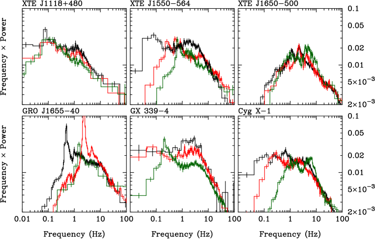
Figure 1: Power density spectra of black hole X-ray binaries. Each panel shows three spectra in the low/hard spectral state, selected from the data analyzed in Sec. 3. The selection demonstrates that despite dramatic changes in the PDS shape at lower frequencies (including variable QPO), the high-frequency part ($\ga$10 Hz) of the PDS remains relatively constant.

Power density spectra of many AGN can be approximated by a broken power law, with power $P_{\nu}\propto\nu^{-1}$ below and $P_{\nu}\propto\nu^{-2}$ above the break frequency, $\nu_{b}$ (e.g. Markowitz et al. 2003b), where $P_{\nu}$ is the power spectral density normalized to the mean and squared. A second break at lower frequencies, below which the power is roughly $P_{\nu}\propto\nu^{0}$, has been also observed (e.g. Pounds et al. 2001; Markowitz, Edelson & Vauhgan 2003a). At the zeroth order of approximation this is consistent with the PDS observed in stellar-mass BHB in the hard spectral state. Fig. 1 shows a sample of PDS from Galactic BHB in the hard state (details of the data reduction are described in Section 3). Plainly, these spectra are much more complex that a doubly-broken power law, with multiple broad and narrow noise components, usually well described by a series of Lorentzians (e.g. Pottschmidt et al. 2003). However, despite this complexity, the entire spectral shape roughly resembles a (doubly) broken power law.

N04 assumed that the break frequency is inversely proportional to the black hole mass, while the $P_{\nu}\propto\nu^{-1}$ part of the PDS below the break (the ‘flat top’ in $\nu P_{\nu}$ diagrams) has constant normalization, independent of the black hole mass. Yet inspection of several BHB power spectra clearly shows that neither of these is constant for a given source. The break frequency is known to change with accretion rate (e.g. Done & Gierliński 2005). The ‘flat top’ normalization can change as well, as one can see in GX 339–4 spectra in Fig. 1.

There is, however, one feature of these power spectra that remains remarkably invariant: the high-frequency spectral shape, above $\nu_{b}$. For a given source it can be roughly described by a single power law with constant index of 1.5–2.0, and constant normalization for various observations differing in luminosity by more than one order of magnitude. In this paper we test the idea that the high-frequency part of the PDS remains fairly constant for a given source and scales with the black hole mass. This is a simple refinement of the idea proposed by N04 and later developed by N06.

Here we do not make any assumptions about how the characteristic frequencies (e.g. break frequency) depend on black hole mass. Instead, we assume that the the PDS above the break frequency (the high-frequency tail) has a universal spectral shape (roughly $\propto\nu^{-2}$) with normalization depending on the black hole mass. This can be written as

$$P_{\nu}=C_{M}(\nu/\nu_{0})^{-2},$$ (1)

where $\nu_{0}$ is an arbitrary frequency which we chose to be $\nu_{0}$ = 1 Hz. Thus, $C_{M}$ (in units of Hz^-1) is the normalization of the (extrapolated) high-frequency tail at 1 Hz.

The assumption that $C_{M}$ is unique function of the black hole mass would directly correspond to the original assumption of N04 about constancy of $P(\nu_{b})\nu_{b}$ if $\nu_{b}$ were constant for a given black hole mass. Due to limited statistics it is often difficult to study details of the high-frequency shape of the PDS. Therefore, we simplify the situation by calculating the amplitude, or the excess variance, of variability in a given frequency band significantly above the break. This can be done directly from a light curve or by integrating the PDS. The excess variance calculated between frequencies $\nu_{1}$ and $\nu_{2}$ (both greater than $\nu_{b}$) is:

$$\sigma_{\rm NXS}^{2}=\int_{\nu_{1}}^{\nu_{2}}P_{\nu}d\nu=C_{M}\nu_{0}\left({\nu_{0}\over\nu_{1}}-{\nu_{0}\over\nu_{2}}\right).$$ (2)

The key assumption, which we want to test in this paper, is that $C_{M}$ is inversely proportional to the black hole mass, $C_{M}=C/M$, where $C$ is a constant. We note that our $C$ is the same constant as constant $C$ defined by N04 in eq. 4, divided by $\nu_{0}^{2}$.

3 Data reduction and selection

Source Name	Start	End
XTE J1118+480	2000-03-29	2000-08-08
	2005-01-13	2005-02-26
4U 1543–47	2002-06-17	2002-10-11
XTE J1550–564	1998-09-07	1999-05-20
	2000-04-10	2000-07-16
	2001-01-28	2001-04-29
	2002-01-10	2002-03-05
	2003-03-27	2003-05-16
XTE J1650–500	2001-09-06	2002-04-21
GRO J1655–40	2005-02-20	2005-11-11
GX 339–4	2002-04-02	2003-05-06
	2003-12-28	2005-08-12
Cyg X-1	1996-02-12	2006-01-12

Table 1: Log of RXTE observations. Each set of data corresponds to one transient outburst. For Cyg X-1 we used all data publicly available in February 2007.

We used publicly available Rossi X-ray Timing Explorer (RXTE) Proportional Counter Array (PCA) data of seven black hole binaries, listed in Table 1. First, we extracted background-corrected energy spectra from Standard-2 data (top layer, detector 2 only) for each pointed observation. These were used to create hardness-intensity diagrams (HID). Intensity is defined as the total 2–60 keV count rate and the hardness ratio is the ratio of count rates in energy bands 6.3–10.5 and 3.8–6.3 keV. We also calculated power density spectra (PDS) for each observation from full-band (2–60 keV) data in 0.0039–128 Hz frequency band. We subtracted the Poissonian noise from the PDS, corrected them for dead-time effects (Revnivtsev, Gilfanov & Churazov 2000) and background (Berger & van der Klis 1994)

We used HIDs to identify hard state spectra. In transients these spectra lie on the vertical branch of the diagram at hardness ratio $\ga$0.8, corresponding to the rise or decay of the outburst. While in GX 339–4 the transition from the vertical hard branch into intermediate horizontal branch is abrupt and well defined, in XTE J1550–564, XTE J1650–500 and GRO J1655–40 we also included a few points from the part of the HID where the hard branch turns into intermediate, as they have sufficiently large hardness ratio to be (potentially) classified as the hard state. In Cyg X-1 we arbitrarily selected observations with hardness ratio greater than 0.9. We also arbitrarily rejected all data with average count rate less than 10 counts per s per PCU as they did not have enough statistics to robustly calculate the high-frequency power. All the selections are shown in Figs. 2 and 3.

For a given source (and separately for each outburst in case of GX 339–4 and XTE J1550–564) we measured the high-frequency power, $\sigma^{2}_{{\rm NXS}}$, with their statistical errors, $\alpha$, for each pointed observation in the hard state. The power (or excess variance) was measured by integrating the PDS over the frequency band 10–128 Hz (eq. 2). Then, we computed the mean amplitude, $\langle C_{M}\rangle$ for a given source (or a particular outburst of the source) weighted by errors of $C_{M}$. The error of $\langle C_{M}\rangle$ was estimated from $\chi^{2}$ statistics for $\Delta\chi^{2}=2.7$, i.e. corresponding to 90 per cent confidence limits.

Despite the initial count rate selection, some data sets (in particular from short observations) gave high-frequency power with large errors. We discarded all these, setting an arbitrary upper limit on error, $\alpha<0.3\sigma^{2}_{{\rm NXS}}$.

4 Results

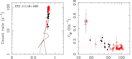
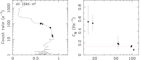
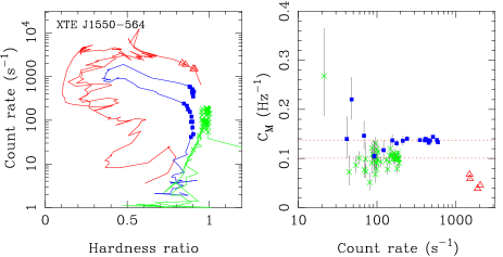
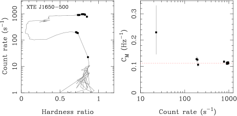
Figure 2: Panels on the left show hardness-intensity diagrams. Solid line shows the entire outburst of a given source, while the data points correspond to the hard-state selection of pointed observations, used for further analysis. Diagrams on the right show the high-frequency variability amplitude, $C_{M}$ (eq. 1), as a function of count rate, for selected hard-state observations. The horizontal line shows the weighted average of $C_{M}$ for the entire outburst. XTE J1118+480 shows data from two outbursts: 2000 (red triangles) and 2005 (black filled squares). XTE J1550–564 diagram shows data from five outbursts: 1998/1999 (red open triangles), 2000 (blue squares) and 2001, 2002 and 2003 together (green crosses). The circled point in XTE J1118+480 panel was used to estimate background effects (see Section 4).

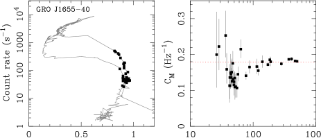
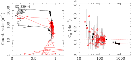
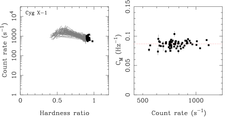
Figure 3: Continuation of Fig. 2. GX 339–4 diagrams shows two outbursts: 2002/2003 (black squares) and 2004 (red triangles).

Figs. 2 and 3 show selection of hard-state data (hardness-intensity diagrams on the left) and measured amplitude of the high-frequency tail, $C_{M}$ in the right-hand panels. It is obvious from these diagrams that $C_{M}$ is not constant for a given source and varies from one pointed observation to another. These variations are not very significant, though. With very few exceptions (2 observations of GRO J1655–40 and 3 of GX 339–4) individual $C_{M}$ measurements are within 3$\sigma$ of the mean. The dispersion is higher in Cyg X-1 where statistics is better and errors on $C_{M}$ smaller. Generally, we find that $C_{M}$ does not significantly depend on the source brightness (count rate).

Source Name	Outburst	$\langle C_{M}\rangle$ (Hz-1)	$T_{\rm hard}$ (days)
XTE J1118+480	2000	$0.098\pm 0.005$	130*
	2005	$0.14\pm 0.02$	26*
4U 1543–47	2002	$0.14\pm 0.01$	–
XTE J1550–564	1998	$\sim$0.05	3
	2000	$0.137\pm 0.002$	14
	2001	$0.095\pm 0.001$	90*
	2002	$0.104\pm 0.004$	50*
	2003	$0.101\pm 0.002$	50*
XTE J1650–500	2001	$0.113\pm 0.001$	8
GRO J1655–40	2005	$0.179\pm 0.003$	12
GX 339–4	2002	$0.088\pm 0.001$	20
	2004	$0.121\pm 0.003$	180
Cyg X-1 (hard)	–	$0.0868\pm 0.0003$	–
Cyg X-1 (soft)	–	$0.139\pm 0.004$	–

Table 2: Mean amplitude of the high-frequency power, $\langle C_{M}\rangle$ (eq. 1). We show data for each outburst separately. $T_{\rm hard}$ is approximate duration of the initial hard state during the rise of the outburst. Asterisks denote hard-state only outbursts. 4U 1543–47 was not observed in the initial hard state and Cyg X-1 is a persistent source.

More significant differences can be found for different outbursts of a given source. We have analyzed five outbursts of XTE J1550–564. The three hard-state outbursts between 2001 and 2003 (see Table 2) were similar in all properties, so we analyzed them together. They yield mean $\langle C_{M}\rangle=0.101\pm 0.002$ Hz^-1. The hard state in 2000 outburst gave higher $\langle C_{M}\rangle=0.137\pm 0.002$ Hz^-1. However, the 1998 outburst was very different, with much lower and quickly changing high-frequency power, $C_{M}\sim 0.05$ Hz^-1. We have excluded the onset of 1998 outburst from further analysis, as it might have represented a different accretion state (we discuss this in detail in Sec. 7). Similarly, GX 339–4 and XTE J1118+480 showed different $C_{M}$ during different outbursts, though at least in the case of the latter one this could have been due to systematic effects at low count rates, which we discuss later in this section.

We looked into the dependence of $C_{M}$ on the hardness ratio, which can be regarded as a crude indicator of the spectral state. We did not find any clear general trend, as illustrated in Fig. 4.

Additionally, we found variability amplitude for three other black hole candidates with no black hole mass estimates. The relatively high value of $\langle C_{M}\rangle=0.15_{-0.04}^{+0.03}$ Hz^-1 obtained for XTE J1720–318 seems to be consistent with a rather low black hole mass of 5 M_⊙, as also suggested by Cadolle Bel (2004) from disc spectral fitting. For H1743–322 (=XTE J1746–322) and XTE J1748-288 we found $\langle C_{M}\rangle=0.090\pm 0.015$ and $0.056\pm 0.008$ Hz^-1, respectively.

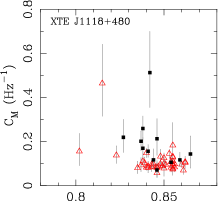
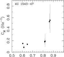
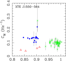
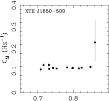
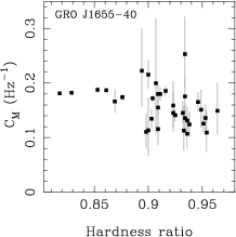
Figure 4: Dependence of amplitude of high-frequency variability, $C_{M}$, on the hardness ratio. There is no clear trend of $C_{M}$ as a function of spectral states.

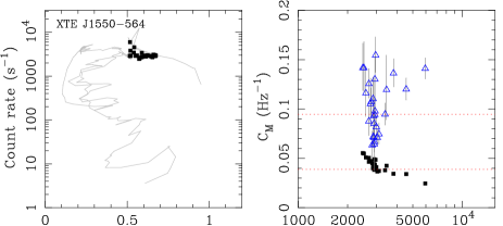
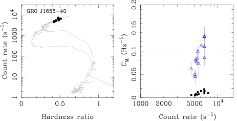
Figure 5: Same as in Figs. 2 and 3, but for the very high (steep power law) spectral state. Black filled squares represent $C_{M}$ calculated from 2–60 keV PCA data, grey (blue in colour) open triangles show the high-energy data (roughly 14–60 keV).

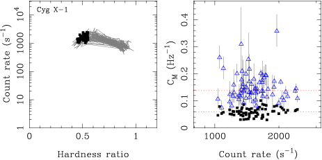
Figure 6: Same as in Fig. 5, but for the soft spectral state of Cyg X-1.

The hard X-ray spectral state, which we study in this paper, is dominated by Comptonized emission. It would be very interesting to see if similar behaviour can be seen in the other spectral state dominated by Comptonization, the very high (or steep power law) state. We have selected the very high state data from hardness-intensity diagrams of XTE J1550–564 and GRO J1655–40, as shown in Fig. 5. These observations have significantly less variability at frequencies $>$10 Hz then the hard state data, so the resulting $C_{M}$ is small (black squares in Fig. 5). But we must remember that the soft X-ray part of the spectrum (where PCA has highest sensitivity) has strong contribution from the cold accretion disc, which can dilute the variability coming from Comptonization (e.g. Done & Gierliński 2005) hence suppressing the observed power. Therefore, we extracted additional power spectra at higher energies (above PCA channel 36, roughly corresponding to energy of 14 keV), where the disc influence is negligible. The high-frequency variability amplitude from these data is much higher, as shown in blue triangles in Fig. 5. Though there is a large scatter in $C_{M}$ from individual observations, the mean $\langle C_{M}\rangle$ is of order of 0.1 Hz^-1 in both sources, consistent with the hard state results. Therefore, the high-frequency variability from Comptonization appears to be very similar in both hard and very high states (but see discussion in Sec. 7).

The soft-state data from our BHB sample are strongly dominated by the disc emission. The only source with reasonable count rates at higher energies in the soft state is Cyg X-1. We applied the same approach to Cyg X-1 soft-state data (arbitrarily chosen hardness ratio in the range 0.45–0.55), as to the very high state data in the previous paragraph. The result can be seen in Fig. 6. The scatter in individual data points in significant, with mean $\langle C_{M}\rangle=0.138\pm 0.004$ Hz^-1. Since the fit of the constant to the data is rather poor, $\chi^{2}_{\nu}$ = 156/73, the error on $\langle C_{M}\rangle$ is indicative only.

5 Caveats

We tested our results for possible systematic effects. Many of our observations have low count rate, which can affect the resulting power spectra. At low count rates, PCA channels 0–7 can create artificial power due to problems with the on-board computer (Revnivtsev, private communication). To test the effect of this we have removed PCA channels 0–7, where PCA configuration allowed for that, and calculated new values of $C_{M}$. We found that this had a negligible effect on our results.

The white noise level was subtracted from the power spectra during data reduction. If the white noise level was not estimated correctly, this could have influenced the amplitude of variability and the resulting $C_{M}$. To test this we have selected observations where high timing resolution was available and calculated power spectra up to 1024 Hz. As we do not expect any significant power above a few hundred Hz from black holes (Sunyaev & Revnivtsev 2000), we assumed that the 512–1024 Hz power could be used as a good white noise estimator. We reanalyzed these data and calculated new values of $C_{M}$. Again, the effect on our results turned out to be negligible.

Background effects can be potentially important for estimating the amplitude of variability, which is defined as $({\rm rms}/{\rm mean})^{2}$. Our power spectra were calculated from light curves not corrected for background, so their power is $[{\rm rms}/(R_{s}+R_{b})]^{2}$, where $R_{s}$ and $R_{b}$ are source and background mean count rates, respectively. These PDS were then multiplied by $[(R_{s}+R_{b})/R_{s}]^{2}$, where source and background count rates were estimated from light curves. In the dimmest observations $R_{s}$ and $R_{b}$ are comparable. To estimate possible background inaccuracy (which is modelled in the PCA rather then measured) we extracted one PCA and HEXTE spectrum (using standard HEASARC reduction techniques, adding 1 per cent systematic errors in the PCA) of XTE J1118+480, corresponding to a high-$C_{M}$ and low count rate point circled in Fig. 2 (ID 90111-01-02-07, observed on 2005-01-24). We have fitted the joined PCA/HEXTE spectrum with a simple Comptonization model (see Done & Gierliński 2003 for details), using PCA in 3–40 and HEXTE in 20–200 keV band. The fit was good ($\chi^{2}=137/145$) with no strong residuals. Then we changed the level of PCA background by $\pm$10 per cent. The fit with 90 per cent of background was only marginally worse ($\chi^{2}=142/145$), while the 110 per cent background resulted in a rather poor fit ($\chi^{2}=171/145$). In both cases there were strong residuals in the PCA and disagreement with HEXTE data above $\sim$25 keV. This shows that the background in the low count rate data is estimated with accuracy much better then 10 per cent. Hence, the uncertainty on $C_{M}$ due to background estimation is no more than a few per cent. The increase of $C_{M}$ by factor 2–5 at low count rates seen in Fig. 2 cannot be caused by incorrect background. Since we see this effect in most sources below the same count rate of $\sim$20 s^-1 (regardless of the distance, hence at different luminosities) it must be of (unknown) instrumental origin. We would like to stress, however, that the increase is not statistically significant, typically less then 2$\sigma$.

The high-frequency variability is known to depend on energy in some sources (e.g. Nowak et al. 1999). This is important when comparing BHB with AGN, as we look at different parts of the Comptonized spectrum, AGN data showing higher scattering orders than BHB. We have tested our data for energy dependence. This was possible only in bright observations from XTE J1550-564, GX 339–4 and Cyg X-1, where statistics at higher energies was good enough. The high-energy (above $\sim$14 keV) data give $\langle C_{M}\rangle=0.13\pm 0.01$ Hz^-1 for the 2000 outburst of XTE J1550–564 and $\langle C_{M}\rangle=0.09\pm 0.01$ Hz^-1 for the 2002 outburst of GX 339–4. These values are consistent with the broad-band data, which in the PCA is dominated by soft X-rays (see Table 2), which suggests that the high-frequency amplitude is not energy-dependent in these sources. On the other hand, similar approach to Cyg X-1 gave $\langle C_{M}\rangle=0.109\pm 0.001$ Hz^-1, higher by about 25 per cent higher then the broad-band data.

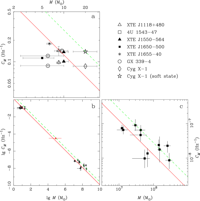
Figure 7: Dependence of $C_{M}$ on black hole mass. Data in the upper left panel show the results of this paper for X-ray binaries. Black hole masses, with references, are listed in Table 3. The lower right panel shows the sample of Seyfert 1 galxies from N06. Black hole masses are obtained from reverberation method (Peterson et al. 2004). The lower left panel show an overview of stellar and supermassive black holes. The red cross in the middle of the diagram represent NGC 4395. The solid red diagonal line shows the best-fitting relation $C_{M}=C/M$, with $C=1.25$ M_⊙ Hz^-1. The green dashed line corresponds to the soft state of Cyg X-1, with $C=2.77$ M_⊙ Hz^-1.

Source Name	$M$ (M⊙)	Reference
XTE J1118+480	8.5 (7.9–9.1)	Gelino et al. (2006)
4U 1543–47	9.4 (7.4–11.4)	Park et al. (2004)
XTE J1550–564	10 (9.7–11.6)	Orosz et al. (2002)
XTE J1650–500	5 (2.7–7.3)	Orosz et al. (2004)
GRO J1655–40	6.3 (5.8–6.8)	Greene, Bailyn & Orosz (2001)
GX 339–4	6 (2.5–10)	Cowley et al. (2002)
Cyg X-1	20 (13.5–29)	Ziółkowski (2005)

Table 3: Black hole masses in X-ray binaries, used in this paper.

6 Dependence on mass

Fig. 7($a$) shows the dependence of $C_{M}$ on black holes mass. We used best currently available mass estimates of black holes in X-ray binaries, as summarized in Table 3. XTE J1650–500 does not have good mass estimate, though Orosz et al. (2004) found an upper limit of 7.4 M_⊙. We assumed the mass function, 2.7 M_⊙, as the lower limit and we adopted the actual mass in the middle of this interval, at 5 M_⊙. We show data from different outbursts of XTE 1118+480, XTE J1550–564 and GX 339–4 separately.

Clearly, there is no apparent correlation between black hole mass and $C_{M}$, though we must bear in mind that mass estimates in X-ray binaries are not very accurate. Moreover, different outbursts giving slightly different $\langle C_{M}\rangle$ create additional dispersion. Hence, the overall uncertainties are rather large, so the expected relation $C_{M}=C/M$ cannot be robustly confirmed from X-ray binaries. To do this, we need to extend our studies to supermassive black holes. N06 compared masses of a sample of Seyfert 1 galaxies measured by reverberation method with masses from high-frequency variability, using the value of constant $C$ derived from Cyg X-1 observations. Here we use the same sample of AGN in order to compare them with our much larger sample of BHB, constrain the $C_{M}=C/M$ relation better and get a ‘big picture’ overview of variability properties for all masses of black holes. In Fig. 7($c$) we plotted the sample of of N06; panel $b$ shows the overview of stellar-mass and supermassive black holes.

The red diagonal line in the diagrams represents the best-fitting function $C_{M}=C/M$, with $C$ = 1.25$\pm 0.06$ M_⊙ Hz^-1. We would like to point out that this particular value depends on the selection of X-ray binary data, as different outbursts can give different $\langle C_{M}\rangle$. Also, errors on mass are non-Gaussian in many cases, so the error on $C$, given here, is indicative only. It is interesting to notice that the constant $C$ is 1.24$\pm$0.06 M_⊙ Hz^-1 for X-ray binaries only and 1.51${}_{-0.29}^{+0.37}$ M_⊙ Hz^-1 for AGN only; both values are consistent within error limits. We also plotted a line (green dashed) corresponding to the soft state of Cyg X-1, for comparison (with $C$ = 2.77 M_⊙ Hz^-1). Some of the AGN are consistent with the soft-state line.

We also tested whether the relation between variability and mass is really linear. We fitted a more general form of a power-law dependence, $C_{M}=C_{f}(M/$M${}_{\odot})^{-\alpha}$ to all BHB and AGN data and found $C_{f}=1.19\pm 0.05$ Hz^-1 and index $\alpha=0.98\pm 0.01$ very close to linear relation. Hence, we opt for the simpler solution and regard the linear relation as well established.

The $C_{M}=C/M$ relation is in excellent agreement with the data spanning over eight orders of magnitude in mass. It gives us robust confirmation of our hypothesis that the high-frequency power is inversely correlated with black hole mass. Even more firm confirmation would come from objects with intermediate black holes mass, filling the big gap in Fig. 7($b$). One category of sources potentially useful for testing this is the ultra-luminous X-ray sources (ULX) with possible masses of hundreds of M_⊙. Alas, they are most likely in the very high spectral state, with soft X-ray emission dominated by the disc. Besides, there are no reliable high-frequency power spectra available from ULX. An interesting source for comparison turns out to be a dwarf galaxy NGC 4395, with black hole mass estimates between 0.13 and 3.6$\times 10^{5}$ M_⊙ (Kraemer et al. 1999; Ho 2002; Filippenko & Ho 2003; Vaughan et al. 2005; Greene & Ho 2006). The luminosity is low, $L/L_{\rm Edd}\la 0.1$ (Vaughan et al. 2005). We analyzed its ASCA observations of 2000-05-24 and 2000-05-26 and found the excess variance for this source and $C_{M}=3.2_{-1.1}^{+1.4}\times 10^{-5}$ Hz^-1. We show the range of masses and $C_{M}$ for NGC 4395 in Fig. 7($b$). They are in excellent agreement with our mass-variability relation! We can also give an independent estimate of the black hole mass in NGC 4395 based on the best-fitting value of $C$: $M\approx 3.9\times 10^{4}$ M_⊙.

7 Discussion

We have analyzed all available hard-state data from seven Galactic black hole systems and found that the amplitude of the high-frequency tail, $C_{M}$, is roughly constant for a given source, changing by no more than a factor two. There is no apparent dependence of $C_{M}$ on luminosity or hardness ratio. This contrasts QPO or break frequency behaviour, which typically show a strong correlation with luminosity. The scale of change of $C_{M}$ is also much less than the observed span of QPO/break frequency, which can be one order of magnitude within the hard state. This makes $C_{M}$ much more invariant feature of a given black hole and a robust estimator of its mass.

There are, certainly, some departures from this rule. Different outbursts of the same transient can have slightly different high-frequency tail amplitudes. Most of the sources show an increase in $C_{M}$ below count rate of $\sim$20 s^-1 per PCU. This might be attributed to systematic instrumental effects at low count rates. Due to large errors this has a negligible effect on our results. But, if this effect extends to higher count rates, than the difference between 2000 and 2005 outbursts of XTE J1118+480 (increase of $C_{M}$ below 40 s^-1, see Fig. 2) could be of instrumental origin.

XTE J1550–564 gives a much clearer exception to this rule. The first outburst in 1998 had a very short initial hard state with the high-frequency tail amplitude much lower than in the next outbursts. In contrast, the three hard-state only outbursts in 2001, 2002 and 2003 produced very consistent results. The explanation of this phenomenon might lie in the stability of the accretion flow. The spectral state during the onset of the 1998 outburst was changing faster than in any other outburst analyzed here and took a different track on the colour-colour diagram (Done & Gierliński 2003). It is possible that the accretion flow during such a rapid transition was in a different state than in slower transitions, possibly due to higher ionization state of the reflector (Wilson & Done 2001; Done & Gierliński 2003). Clearly, this also affected its variability properties, decreasing the high-frequency power. This particular hard state was different in many aspects, so we rejected it from our sample. The more stable hard-state only outbursts give probably a better estimate of $C_{M}$. Similarly, the persistent source, Cyg X-1, gave a very stable and robust high-frequency power.

Thus, fast transitions, characterized by an unstable and quickly changing accretion flow, can apparently break the $C_{M}=C/M$ law. In Table 2 we show the approximate duration of the initial hard state after the onset of the outburst. XTE J1650–500 showed a rather quick transition, so might have suffered from a similar instability, as XTE J1550–564 in 1998. On the other hand, the tail amplitude was very stable and returned to the same level in the hard state at the end of the outburst (see Fig. 2). The 2004/2005 outburst of GX 339–4 had a much longer hard state than the 2002/2003 outburst, so perhaps it was a better estimate of the high-frequency power.

In this work we assumed the constant power-law high-frequency tail with the spectral index of -2. This is not necessarily true and detailed fits to PDS of X-ray binaries, where statistics is sufficient, show indices between 1.5 and 2.0. We note that the particular choice of the spectral index does not affect the overall result of our paper, as different index would only introduced a constant offset in $C_{M}$. Scatter in spectral indices from one observation to another might introduce some additional uncertainty, though this would be very difficult to estimate for AGN.

The luminosities of the Seyfert 1 sample used in this paper are generally low, $\la$5 per cent of $L_{\rm Edd}$, except for 3C120 and NGC 7469, which are significantly brighter. The 3–10 keV photon power-law indices are $\Gamma\sim$ 1.5–1.8 (Nandra et al. 1997). This suggests that these sources are in the hard X-ray spectral state. On the other hand, the spectral index of Comptonized component alone is not enough to establish the X-ray spectral state. Many BHB show soft-state disc-dominated spectra with a flat ($\Gamma\approx 2$) power-law Comptonized tail, while measuring the intrinsic spectral index in AGN is not straightforward due to presence of complex absorption and/or reflection (Gierliński & Done 2004). We cannot rule out (in particular for brighter AGN) that some of the sources in the sample are actually in the soft X-ray spectral state. Despite that the mass-variability amplitude correlation seems to hold well for all of them. Some of the objects are more consistent with the soft-state Cyg X-1 line in Fig. 7($c$). On the other hand, the brightest 3C120 and NGC 7469 lay below the hard-state line. Clearly, the dependence of high-frequency amplitude on luminosity and spectral state in AGN requires further studies.

Our analysis of the very high (steep power law) state shows that after a simple bandwidth correction the tail power is consistent with the hard-state results. This is very encouraging, showing that perhaps the universal shape of the high-frequency tail is the inherent property of Comptonization, regardless of the spectral state. Narrow-line Seyfert 1 galaxies (NLS1) are most likely the supermassive counterparts of Galactic sources in the bright very high state (e.g. Pounds, Done & Osborne 1995). N04, and later Nikołajuk, Gurynowicz & Czerny (2007) showed that the excess variance from the NLS1 sample is by a factor $\sim$20 larger than expected from $C_{M}=C/M$ correlation established for moderate-luminosity AGN. NLS1 have also systematically higher break frequencies for a given mass, so the luminosity dependence of the break frequency (M^cHardy et al. 2006) can perhaps be related to the increase in $C_{M}$. One explanation could be a bandpass effect. The seed photons in X-ray binaries in the very high state are at $\sim$1 keV, while in AGN they are at much lower energies, $\la$10 eV. Therefore, we see a different part of the Comptonized spectrum in X-rays. Gierliński & Zdziarski (2005) showed that the variability amplitude strongly increases with energy in the very high state, while it is almost constant in the hard state. As we see higher orders of scattering in NLS1 than in the very-high-state stellar mass black holes, we expect higher variability in the former ones, as observed. Another possible explanation is contribution from complex absorption to the observed variability, which can significantly increase the rms at energies $\sim$1–2 keV (Markowitz et al. 2003a; Gierliński & Done 2006). We expect more complex absorption from bright NLS1 sources with strong outflows. The low- and moderate-luminosity AGN are less likely to be affected by this additional variability.

Fig. 7 shows that the amplitude of the high-frequency tail in the PDS scales very well with the black hole mass. The correlation holds for over seven orders of magnitude. Thus, the high-frequency power in accreting black holes in the hard spectral states seems to be universal. This part of the PDS corresponds to the shortest timescales producing power in the accretion flow. Features (e.g. QPOs) occasionally observed at higher frequencies (e.g. Strohmayer 2001) have much less power. We do not understand the origin of rapid X-ray variability from accretion flows very well. It might be created by fluctuations propagating in the accretion flow (Lyubarskii 1997). The closer to the centre, the shorter characteristic timescales of fluctuations. Inevitable, there is a final barrier for propagation, the last stable orbit, which acts as a low-pass filter, removing all frequencies higher than a certain limit. The limiting frequency is inversely proportional to the radius of the last stable orbit and hence to the black hole mass. With a certain shape of the filter any initial spectrum of fluctuations will be truncated to a similar shape at higher frequencies. This might (at least qualitatively) explain the observed universal shape of the high-frequency tail (Done, Gierliński & Kubota 2007).

Obviously, the size of the last stable orbit depends not only on the black hole mass, but also on its spin. Higher spin would shrink the last stable orbit as if the black hole mass was smaller. This would increase $C_{M}$ by factor 4.8 for a maximally spinning Kerr black hole with respect to a Schwarzschild one. Alas, the black hole spin is notoriously difficult to measure (compare, e.g., McClintock et al. 2006 and Middleton, Done & Gierliński 2006). The potentially highly spinning GRS 1915+105 has never been observed in the low-luminosity hard spectral state. Another culprit is XTE J1650–500, in which a broad iron line, suggesting high black hole spin, has been reported (Miller et al. 2002, but see also Done & Gierliński 2006). However, as one can see in Fig. 7 $C_{M}$ of this source is well below the $C/M$ line, so its high spin does not seem to be supported by our data. On the other hand the mass of black hole in this source is not very well established, so we cannot make any strong statements about it. Fig. 7 shows that the scatter in $C_{M}$ for all sources is only factor two, so we do not expect large scatter in black hole spins in the sample.

Yet another factor that might influence the results is the inclination of the disc with respect to the observer. If rapid X-ray variability is produced in flares or fluctuations corotating with the disc, then it is affected by Doppler effects for highly inclined discs. Życki & Niedźwiecki (2005) calculated these effects and predicted that high inclinations would give rise to strong increase in the high-frequency power. However, the additional signal appears above $\sim$100 Hz and would not be easily detected in PDS. We calculated $C_{M}$ from 10–128 Hz band, so our results should not be affected by the inclination.

8 Comparison with break-frequency scaling

An alternative approach of linking variability with black hole mass is the mass-luminosity-break frequency scaling, $\nu_{b}=AL_{\rm bol}^{B}/M^{C}$ (M^cHardy et al. 2006; Körding et al. 2007), where the three observables: mass, luminosity and break frequency form a ‘fundamental plane’ along which the BHB and AGN data correlate.

We would like to point out few advantages of the method proposed in this paper over the break-frequency scaling. Generally, it is easier to find variability amplitude than the break frequency, as the latter requires modelling of the power spectrum (but see Pessah 2007). The amplitude method does not involve luminosity or accretion rate, so it doesn’t require distance to the source, which in case of many Galactic black holes is poorly constrained. Another advantage of this approach is its simplicity, as it relates amplitude of variability with black hole mass directly, with just one scaling constant. The break-frequency method requires three independent constants. This suggests that high-frequency variability amplitude is more fundamental in nature.

One of the drawbacks of the amplitude method is its limitation to the hard X-ray spectral state in BHB. Another state dominated by Comptonization, the very high (steep power law) state is potentially useful, but its application to bright AGN requires better understanding of energy dependence of rms. Soft-state spectra of BHB are strongly diluted by the (stable) disc and good-statistics high-energy data, required to establish $C_{M}$ reliably, is not available (except for Cyg X-1 and, perhaps, GRS 1915+105). But most of the AGN spectra in the 2–10 keV band are dominated by Comptonization, so this method might be valid in the soft state. The same problem seems to affect the break-frequency scaling. Körding et al. (2007) point out that their method is mostly limited to the hard state, as measuring and defining the break frequency in soft and very high states is very difficult.

Both break-frequency and amplitude correlations require a shift in the relation when applied to Cyg X-1 in the soft spectral state (Körding et al. 2007), though this is rather difficult to extend to soft states of other BHB.

The high-frequency amplitude depends, to some extend, on energy, while the break-frequency is energy-independent. Another potential disadvantage of the amplitude method is additional variability introduced by ionized smeared absorption or reflection in some sources, which is most pronounced around 1–2 keV (Markowitz et al. 2003b; Gierliński & Done 2006; Crummy et al. 2006).

9 Conclusions

Black hole X-ray binaries have a universal shape of the high-frequency tail (above the break frequency) in their PDS, as illustrated in Fig. 1. Though the exact shape of the tail is not easy to establish, it can be approximated by a power law, $P_{\nu}=C_{M}(\nu/\nu_{0})^{-2}$. The amplitude, $C_{M}$ of the tail is remarkably constant for any given BHB in the hard state, regardless of the luminosity. When extended to supermassive black holes in moderate luminosity AGN, the tail amplitude scales very well with black hole mass, $C_{M}=C/M$. The best-fitting value of the scaling constant from our sample of BHB and AGN is $C$ = 1.25$\pm 0.06$ M_⊙ Hz^-1. This method can be applied to estimate black hole masses in many AGN. If the universal shape of the high-frequency tail is an inherent property of Comptonization, it might be applied to other spectral states. We speculate that the constancy of the tail is an imprint of the last stable orbit around the black hole.

References

- [\citeauthoryearBerger & van der Klis1994] Berger M., van der Klis M., 1994, A&A, 292, 175
- [\citeauthoryearCadolle Bel et al.2004] Cadolle Bel M., et al., 2004, A&A, 426, 659
- [\citeauthoryearCowley et al.2002] Cowley A. P., Schmidtke P. C., Hutchings J. B., Crampton D., 2002, AJ, 123, 1741
- [\citeauthoryearCrummy et al.2006] Crummy J., Fabian A. C., Gallo L., Ross R. R., 2006, MNRAS, 365, 1067
- [\citeauthoryearCzerny et al.2001] Czerny B., Nikołajuk M., Piasecki M., Kuraszkiewicz J., 2001, MNRAS, 325, 865
- [\citeauthoryearDone & Gierliński2003] Done C., Gierliński M., 2003, MNRAS, 342, 1041
- [\citeauthoryearDone & Gierliński2005] Done C., Gierliński M., 2005, MNRAS, 364, 208
- [\citeauthoryearDone & Gierliński2006] Done C., Gierliński M., 2006, MNRAS, 367, 659
- [\citeauthoryearDone, Gierlinski, & Kubota2007] Done C., Gierliński M., Kubota A., 2007, A&AR, in press, arXiv:0708.0148
- [Filippenko & Ho(2003)] Filippenko, A. V., & Ho, L. C. 2003, ApJ, 588, L13
- [\citeauthoryearGelino et al.2006] Gelino D. M., Balman Ş., Kızıloğlu Ü., Yılmaz A., Kalemci E., Tomsick J. A., 2006, ApJ, 642, 438
- [\citeauthoryearGierliński & Done2004] Gierliński M., Done C., 2004, MNRAS, 349, L7
- [\citeauthoryearGierliński & Zdziarski2005] Gierliński M., Zdziarski A. A., 2005, MNRAS, 363, 1349
- [\citeauthoryearGierliński & Done2006] Gierliński M., Done C., 2006, MNRAS, 371, L16
- [Greene & Ho(2006)] Greene, J. E., & Ho, L. C. 2006, ApJ, 641, L21
- [\citeauthoryearGreene, Bailyn, & Orosz2001] Greene J., Bailyn C. D., Orosz J. A., 2001, ApJ, 554, 1290
- [\citeauthoryearHayashida et al.1998] Hayashida K., Miyamoto S., Kitamoto S., Negoro H., Inoue H., 1998, ApJ, 500, 642
- [Ho(2002)] Ho, L. C. 2002, ApJ, 564, 120
- [\citeauthoryearKörding et al.2007] Körding E. G., Migliari S., Fender R., Belloni T., Knigge C., McHardy I., 2007, MNRAS, 380, 301
- [Kraemer et al.(1999)] Kraemer, S. B., Ho, L. C., Crenshaw, D. M., Shields, J. C., & Filippenko, A. V. 1999, ApJ, 520, 564
- [\citeauthoryearLu & Yu2001] Lu Y., Yu Q., 2001, MNRAS, 324, 653
- [\citeauthoryearLyubarskii1997] Lyubarskii Y. E., 1997, MNRAS, 292, 679
- [\citeauthoryearMarkowitz & Edelson2001] Markowitz A., Edelson R., 2001, ApJ, 547, 684
- [\citeauthoryearMarkowitz & Uttley2005] Markowitz A., Uttley P., 2005, ApJ, 625, L39
- [\citeauthoryearMarkowitz, Edelson, & Vaughan2003] Markowitz A., Edelson R., Vaughan S., 2003a, ApJ, 598, 935
- [\citeauthoryearMarkowitz et al.2003] Markowitz A., et al., 2003b, ApJ, 593, 96
- [\citeauthoryearMcClintock et al.2006] McClintock J. E., Shafee R., Narayan R., Remillard R. A., Davis S. W., Li L.-X., 2006, ApJ, 652, 518
- [\citeauthoryearMcHardy et al.2004] McHardy I. M., Papadakis I. E., Uttley P., Page M. J., Mason K. O., 2004, MNRAS, 348, 783
- [\citeauthoryearMcHardy et al.2006] McHardy I. M., Koerding E., Knigge C., Uttley P., Fender R. P., 2006, Natur, 444, 730
- [\citeauthoryearMiddleton et al.2006] Middleton M., Done C., Gierliński M., Davis S. W., 2006, MNRAS, 373, 1004
- [\citeauthoryearMiller et al.2002] Miller J. M., et al., 2002, ApJ, 570, L69
- [\citeauthoryearNandra et al.1997] Nandra K., George I. M., Mushotzky R. F., Turner T. J., Yaqoob T., 1997, ApJ, 477, 602
- [\citeauthoryearNikołajuk, Papadakis, & Czerny2004] Nikołajuk M., Papadakis I. E., Czerny B., 2004, MNRAS, 350, L26 (N04)
- [] Nikołajuk M., Gurynowicz P., Czerny B., 2007, preprint, astro-ph/0612376
- [\citeauthoryearNikołajuk et al.2006] Nikołajuk M., Czerny B., Ziółkowski J., Gierliński M., 2006, MNRAS, 370, 1534 (N06)
- [\citeauthoryearNowak et al.1999] Nowak M. A., Vaughan B. A., Wilms J., Dove J. B., Begelman M. C., 1999, ApJ, 510, 874
- [\citeauthoryearOrosz et al.2002] Orosz J. A., et al., 2002, ApJ, 568, 845
- [\citeauthoryearOrosz et al.2004] Orosz J. A., McClintock J. E., Remillard R. A., Corbel S., 2004, ApJ, 616, 376
- [\citeauthoryearPapadakis2004] Papadakis I. E., 2004, MNRAS, 348, 207
- [\citeauthoryearPark et al.2004] Park S. Q., et al., 2004, ApJ, 610, 378
- [\citeauthoryearPessah2007] Pessah M. E., 2007, ApJ, 655, 66
- [Peterson et al.(2005)] Peterson, B. M., et al. 2005, ApJ, 632, 799
- [\citeauthoryearPottschmidt et al.2003] Pottschmidt K., et al., 2003, A&A, 407, 1039
- [\citeauthoryearPounds, Done, & Osborne1995] Pounds K. A., Done C., Osborne J. P., 1995, MNRAS, 277, L5
- [\citeauthoryearRevnivtsev, Gilfanov, & Churazov2000] Revnivtsev M., Gilfanov M., Churazov E., 2000, A&A, 363, 1013
- [\citeauthoryearStrohmayer2001] Strohmayer T. E., 2001, ApJ, 552, L49
- [\citeauthoryearSunyaev & Revnivtsev2000] Sunyaev R., Revnivtsev M., 2000, A&A, 358, 617
- [\citeauthoryearVaughan et al.2005] Vaughan S., Iwasawa K., Fabian A. C., Hayashida K., 2005, MNRAS, 356, 524
- [\citeauthoryearWilson & Done2001] Wilson C. D., Done C., 2001, MNRAS, 325, 167
- [\citeauthoryearZiółkowski2005] Ziółkowski J., 2005, MNRAS, 358, 851
- [\citeauthoryearŻycki & Niedźwiecki2005] Życki P. T., Niedźwiecki A., 2005, MNRAS, 359, 308