The Initial-Final Mass Relationship from white dwarfs in common proper motion pairs^⋆

Abstract

Context. The initial-final mass relationship of white dwarfs, which is poorly constrained, is of paramount importance for different aspects in modern astrophysics. From an observational perspective, most of the studies up to now have been done using white dwarfs in open clusters.

Aims. In order to improve the initial-final mass relationship we explore the possibility of deriving a semi-empirical relation studying white dwarfs in common proper motion pairs. If these systems are comprised of a white dwarf and a FGK star, the total age and the metallicity of the progenitor of the white dwarf can be inferred from the detailed analysis of the companion.

Methods. We have performed an exhaustive search of common proper motion pairs containing a DA white dwarf and a FGK star using the available literature and crossing the SIMBAD database with the Villanova White Dwarf Catalog. We have acquired long-slit spectra of the white dwarf members of the selected common proper motion pairs, as well as high resolution spectra of their companions. From these observations, a full analysis of the two members of each common proper motion pair leads to the initial and final masses of the white dwarfs.

Results. These observations have allowed us to provide updated information for the white dwarfs, since some of them were misclassified. In the case of the DA white dwarfs, their atmospheric parameters, masses, and cooling times, have been derived using appropriate white dwarf models and cooling sequences. From a detailed analysis of the FGK stars spectra we have inferred the metallicity. Then, using either isochrones or X-ray luminosities we have obtained the main-sequence lifetime of the progenitors, and subsequently their initial masses.

Conclusions. This work is the first one in using common proper motion pairs to improve the initial-final mass relationship, and has also allowed to cover the poorly explored low-mass domain. As in the case of studies based on white dwarfs in open clusters, the distribution of the semi-empirical data presents a large scatter, which is higher than the expected uncertainties in the derived values. This suggests that the initial-final mass relationship may not be a single-valued function.

1 Introduction

White dwarfs are the final remnants of low- and intermediate-mass stars. About 95% of main-sequence stars will end their evolutionary pathways as white dwarfs and, hence, the study of the white dwarf population provides details about the late stages of the life of the vast majority of stars. Since white dwarfs are long-lived objects, they also constitute useful objects to study the structure and evolution of our Galaxy (Liebert et al. 2005a; Isern et al. 2001). For instance, the initial-final mass relationship (IFMR), which connects the properties of a white dwarf with those of its main-sequence progenitor, is of paramount importance for different aspects in modern astrophysics. It is required as an input for determining the ages of globular clusters and their distances, for studying the chemical evolution of galaxies, and also to understand the properties of the Galactic population of white dwarfs. Despite its relevance, this relationship is still poorly constrained, both from the theoretical and the observational points of view.

The first attempt to empirically determine the initial-final mass relationship was undertaken by Weidemann (1977), who also provides a recent review on this subject (Weidemann 2000). It is still not clear how this function depends on the mass and metallicity of the progenitor, its angular momentum, or the presence of a strong magnetic field. The total age of a white dwarf can be expressed as the sum of its cooling time and the main-sequence lifetime of its progenitor. The latter depends on the metallicity of the progenitor of the white dwarf, but it cannot be determined from observations of single white dwarfs. This is because white dwarfs have such strong surface gravities that gravitational settling operates very efficiently in their atmospheres, and any information about their progenitors (e.g. metallicity) is lost in the very early evolutionary stages of the cooling track. Moreover, the evolution during the AGB phase of the progenitors is essential in determining the size and composition of the atmospheres of the resulting white dwarfs, since the burning processes that take place in H and He shells determine their respective thicknesses and their detailed chemical compositions, which are crucial ingredients for determining the evolutionary cooling times.

A promising approach to circumvent the problem, and also to directly test the initial-final mass relationship, is to study white dwarfs for which external constraints are available. This is the case of white dwarfs in open and globular clusters (Ferrario et al. 2005, Dobbie et al. 2006) or in non-interacting binaries, for instance, common proper motion pairs (Wegner 1973, Oswalt et al. 1988). Focusing on the latter, it is sound to assume that the members of a common proper motion pair were born simultaneously and with the same chemical composition. Since the components are well separated (100 to 1000 AU), mass exchange between them is unlikely and it can be considered that they have evolved as isolated stars. Thus, important information of the white dwarf, such as its total age or the metallicity of the progenitor, can be inferred from the study of the companion. In particular, if the companion is an F, G or K type star the metallicity can be derived with high accuracy from detailed spectral analysis. On the other hand, the age can be obtained using different methods. In particular, we will use stellar isochrones when the star is moderately evolved, or the X-ray luminosity if the star is very close to the ZAMS.

The purpose of this work is to present our spectroscopic analysis of both members of some common proper motion pairs containing a white dwarf, and the semi-empirical intial-final mass relationship that we have derived from this study. The paper is organized as follows. In §2 we present the observations done so far and describe the data reduction. Section 3 is devoted to discuss the classification and the analysis of the observed white dwarfs, whereas in §4 we present the analysis of the companions. This is followed by §5 where we present our main results and finally in §6 we elaborate our conclusions.

2 Observations and data reduction

The sample of common proper motion pairs to be observed was chosen from the available literature, mainly from the papers of Silvestri et al. (2001) and Wegner & Reid (1991), and from a cross-correlation of the SIMBAD database and the Villanova White Dwarf Catalog. We selected the pairs taking into account different requirements. Firstly, the white dwarf component should be classified as a DA (i.e., with the unique presence of Balmer lines), so that the fitting procedure is sufficiently accurate to derive realistic values for the effective temperature and surface gravity. Secondly, the other component of the pair should be a star of spectral type F, G or K for an accurate determination of the metallicity, and moderately evolved or very close to the ZAMS in order to be able to estimate its age. The complete list of targets is given in Table 1.

The observations were carried out during different campaigns between the summer of 2005 and the spring of 2007. In Table 2 we give details of the telescope-instrument configurations employed, as well as the resolution and spectral coverage of each setup.

For the white dwarf members we performed long-slit low-resolution spectroscopic observations covering some of the main Balmer lines (from H$\beta$ to H$8$). WD0315$-$011 was kindly observed for us by T. Oswalt with the RC spectrograph at the 4 m telescope at Kitt Peak National Observatory with a resoltuion of about $1.5$ Å  FWHM. We performed as many exposures as necessary to guarantee a high signal-to-noise ratio final spectrum for each object (after the corresponding reduction). Spectra of high quality are essential to derive the atmospheric parameters with accuracy. We co-added individual 1800 s  exposures to minimize the effects of cosmic ray impacts on the CCD.

The white dwarf spectra were reduced using the standard procedures within the single-slit tasks in IRAF. First, the images were bias- and flatfield-corrected, and then, the spectra were extracted and wavelength calibrated using arc lamp observations. We combined multiple spectra of the same star to achieve a final spectrum of high signal-to-noise ratio (S/N $>$ 100). Before this step, we applied the heliocentric correction of each spectrum, since we were co-adding spectra secured in different days. Finally, they were normalized to the continuum.

The FGK companions were observed with echelle spectrographs, obtaining high signal-to-noise high-resolution spectra (S/N $>$ 150), which are necessary to derive the metallicity with accuracy. For the reduction of the FGK stars spectra the procedure followed was similar to the case of white dwarfs but we used the corresponding echelle tasks in IRAF. In this case, we used the task apscatter in order to model and subtract the scattered light.

Table 1: Common proper motion pairs studied in this work.

System	White Dwarf	Companion	Sp. Type1
G 158$-$78/77	WD0023$-$109	G158$-$77	K
LP 592$-$80/	WD0315$-$011	BD $-$01 469A	K1IV
LTT 1560
GJ 166 A/B	WD0413$-$077	HD 26965	K1V
G 116$-$16/14	WD0913$+$442	BD $+$44 1847	G0
G 163$-$B9B/A	WD1043$-$034	G163$-$B9A	F9V
LP 378$-$537	WD1304$+$227	BD $+$23 2539	K0
G 165$-$B5B/A	WD1354$+$340	BD $+$34 2473	F8
G 66$-$36/35	WD1449$+$003	G66$-$35	G5V
EGGR 113/	WD1544$+$008	BD $+$01 3129	G0
BD $+$01 3129
GJ 599 A/B	WD1544$-$377	HD 140901	G6V
GJ 620.1 B/A	WD1620$-$391	HD 147513	G5V
GJ 2125 / GJ 3985	WD1659$-$531	HD 153580	F6V
G 140$-$B1B/	WD1750$+$098	BD $+$09 3501	K0
BD $+$09 3501
G 156$-$64/65	WD2253$-$081	BD $-$08 5980	G6V

From SIMBAD database.

Table 2: Journal of observations.

Observatory	Telescope	Spectrograph	R	Spectral
				Coverage
		White Dwarfs
McDonald	2.7 m HJS	LCS	1,000	3885$-$5267 Å
CAHA	3.5 m	TWIN	1,250	3570$-$5750 Å
LCO	6.5 m Clay	LDSS3	1,650	3600$-$6000 Å
		Low-mass Companions
McDonald	2.7 m HJS	2dcoudé	60,000	3400$-$10900 Å
CAHA	2.2 m	FOCES	47,000	3600$-$9400 Å
ORM	3.5 m TNG	SARG	57,000	4960$-$10110 Å
LCO	6.5 m Clay	MIKE	65,000	4900$-$10000 Å

3 White dwarf analysis

3.1 Classification

Table 3: Spectral classification of the white dwarfs.

Name	This Work	Previous	Reference
WD0023$-$109	DA	DA	EG65, WR91, OS94, MS99
WD0315$-$011	DA	DA	OS94, MS99, SOW01
WD0413$-$077	DA	DA	EG65, FKB97, MS99, HOS02, HBB03, KNH05, HB06
WD0913$+$442	DA	DA	EG65, WR91, BLF95, BLR01, ZKR03, KNH05, LBH05, HB06
WD1043$-$034	sdB1	DA/sd	WR91
		DAB	OS94, MS99
WD1304$+$227	DA	DA	O81, OS94, MS99, SOW01
WD1354$+$340	DA	DA	EG67, WR91, BLF95, MS99, SOW01
WD1449$+$003	M	DA	O81, WR91, OS94
		M	FBZ05
WD1544$+$008	sdO1	DA/sdO	W91
		DA	EG65, MS99
		DAB	SOW01
WD1544$-$377	DA	DA	EG65, W73, OS94, PSH98, BLR01, KNC01, SOW01
		DA	HOS02, HBB03, ZKR03, KNH05, KVS07
WD1620$-$391	DA	DA	W73, OS94, HBS98, PSH98, SOW01, HOS02, HBB03, HB06, KVS07
WD1659$-$531	DA	DA	W73, OS94, PSH98, SOW01, KVS07
WD1750$+$098	DC	DA	WR91, SOW01
		DC	EG65, OS94, MS99
WD2253$-$081	DA	DA	OS94, BLF95, MS99, BLR01, KNC01, SOW01, KNH05

P. Bergeron, private communication.

References. (BLF95) Bergeron et al. (1995); (BLR01) Bergeron et al. (2001); (EG65) Eggen & Greenstein (1965); (EG67) Eggen & Greenstein (1967); (FBZ05) Farihi et al. (2005); (FKB97) Finley et al. (1997); (HOS02) Holberg et al. (2002); (HBB03) Holberg et al. (2003); (HB06) Holberg & Bergeron (2006); (KNC01) Koester et al. (2001); (KNH05) Karl et al. (2005); (KVS07) Kawka et al. (2007); (MS99) McCook & Sion (1999); (O81) Oswalt (1981); (OS94) Oswalt & Strunk (1994); (PSH98) Provencal et al. (1998); (SOW01) Silvestri et al. (2001); (W73) Wegner (1973); (WR91) Wegner & Reid (1991); (ZKR03) Zuckerman et al. (2003)

After the corresponding reduction, we carried out a first inspection of the spectra. All the objects in Table 3 were previously classified as DA white dwarfs. However, we found that four of them are not of DA type. Particularly, WD1750$+$098 turned out to be of type DC although in the most recent reference (Silvestri et al. 2001) it appears classified as a DA. We believe that WD1544$+$008 is the same star as WD1544$+$009, which was classified as a DAB white dwarf by Silvestri et al. (2001). However, it was identified as a sdO star by Wegner & Reid (1991). The same authors also studied WD1043$-$034 and classified it as a sdB star, although McCook & Sion (1999) considered it as a DAB white dwarf. Taking into account the different inconsistencies in the literature, we decided to reobserve these objects in order to revise their spectral classifications, if necessary. The reduced spectra of these two stars were kindly analysed by P. Bergeron, who performed the corresponding fits and derived their temperatures and surface gravities, which turned out to be too low to be white dwarfs. As can be seen in Table 3, WD1449$+$003 is an M star. This classification was also recently indicated by Farihi et al. (2005). These authors also reported that WD0913$+$442 and BD $+$44 1847 are not a physical pair according to their parallaxes. It is worth mentioning that some of the previous misclassifications are probably due to the fact that the signal-to-noise ratio of the spectra used was low.

3.2 Atmospheric parameters

Table 4: Atmospheric parameters derived for the observed white dwarfs.

Name	$T_{\rm eff}$ (K)	$\log g$ (dex)
WD0023$+$109	$10380\pm 230$	$7.92\pm 0.08$
WD0315$-$011	$7520\pm 260$	$8.01\pm 0.45$
WD0413$-$0771	$16570\pm 350$	$7.86\pm 0.05$
WD0913$+$442	$8920\pm 110$	$8.29\pm 0.10$
WD1304$+$227	$10800\pm 120$	$8.21\pm 0.05$
WD1354$+$340	$13650\pm 420$	$7.80\pm 0.15$
WD1544$-$377	$10600\pm 250$	$8.29\pm 0.05$
WD1620$-$391	$24900\pm 130$	$7.99\pm 0.03$
WD1659$-$531	$14510\pm 250$	$8.08\pm 0.03$
WD2253$-$081	$7220\pm 140$	$8.25\pm 0.20$

We do not have a spectrum of this star. These values are from Heber et al. (1997) and Bergeron et al. (1995).

Before calculating the atmospheric parameters of the white dwarfs ($T_{\rm eff}$ and $\log g$) we determined the radial velocities of each star using the IRAF task fxcor. Each spectrum was cross-correlated with a reference model from a grid computed by D. Koester (private communication). The obtained radial velocities, estimated with large error bars, were generally small (ranging from 10 to 50 km/s) compared with the resolution element (300 km/s) of our observations. In only one case (WD0023$+$109), the radial velocity measured turned out to be relevant (150 km/s). However, all radial velocities were taken into account for consistency.

After this previous step, we derived the atmospheric parameters of these stars performing a fit of the observed Balmer lines to white dwarf models following the procedure described in Bergeron et al. (1992). The models had been previously normalized to the continuum and convolved with a Gaussian instrumental profile with the proper FWHM in order to have the same resolution as the observed spectra. The fit of the line profiles was then carried out using the task specfit of the IRAF package, which is based on $\chi^{2}$ minimization with the Levenberg-Marquardt method. We used specfit for different $\log g$ values (7.0, 7.5, 8.0, 8.5 and 9.0) with $T_{\rm eff}$ as a free parameter, obtaining different $\chi^{2}$ for each fit. In each case, the initial estimate for $T_{\rm eff}$ obtained from the spectral energy distribution (photometry in the $BV$ and $JHK$ bands, 2MASS) was used as a starting guess. The uncertainties in the derived $T_{\rm eff}$ were estimated from the perturbations required to increase the value of the reduced $\chi^{2}$ by one.

The determination of $\log g$ was performed in an analogous way but to calculate the errors we took into account the prescription of Bergeron et al. (1992), who derive them from the independent fits of the individual exposures for any given star (before the combination). The results are given in Table 4. In Fig. 1 we show the fits for some of the DA white dwarfs in our sample.

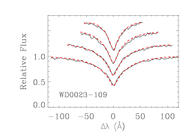
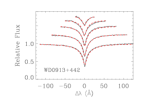
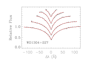
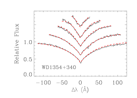
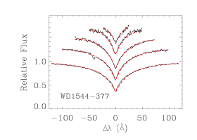
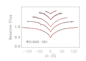
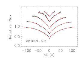
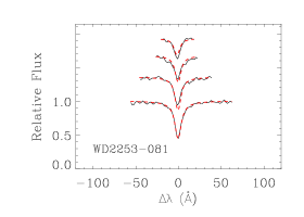
Figure 1: Fits of the observed Balmer lines for the white dwarfs studied here. Lines range from H$\beta$ (bottom) to H$8$ (top), except for WD0023$-$109 and WD2253$-$081 (to H$\varepsilon$).

Some of these white dwarfs had been the subject of previous analyses which allow us to perform a comparison with our results. For instance, WD0913$+$442 was also studied by Bergeron et al. (1995), who obtained atmospheric parameters compatible with the ones derived here. They also studied WD1354$+$340 and WD2253$-$081, but in these cases the effective temperatures obtained are compatible with ours while the surface gravities are not, although just outside the $1\sigma$ error bar. We have obtained lower values of $\log g$ in both cases, which could be due to the different resolution of the spectra ($\sim 6$ FHWM in their case). This latter object, WD2253$-$081, is of particular interest since an accurate fit of its line profiles posed many problems to previous analyses because the lines seemed to be broader than the models predicted. This led different authors to consider the possibility of this star to be a magnetic white dwarf or to have its lines rotationally broadened. Both options were considered by Karl et al. (2005), who discarded the former possibility. With the purpose of solving the fitting problem of this star, in this work we have used updated models for DA white dwarfs with effective temperatures between 6000 and 10000 K. These models were kindly provided by D. Koester, who calculated them considering collision-induced absorption due to the presence of molecular hydrogen. This effect is very significant at low temperatures and it should be taken into account for an accurate determination of the atmospheric parameters. Contrarily to the results obtained by Karl et al. (2005) we did not need to consider rotational broadening to achieve a good fit. On the other hand, the southern hemisphere targets had been also studied by different authors. Recently, Kawka et al. (2007) derived the atmospheric parameters for WD1544$-$377, WD1620$-$391 and WD1659$-$531, which are in good agreement with our results.

3.3 Masses and cooling times

Once we have derived the $T_{\rm eff}$ and $\log g$ of each star, we can obtain its mass ($M_{\rm WD}$) and cooling time ($t_{\rm cool}$) from appropriate cooling sequences. We have used the cooling tracks of Salaris et al. (2000) — model S0 — which consider a carbon-oxygen (C/O) core white dwarf (with a higher abundance of O at the center of the core) with a thick hydrogen envelope on top of a helium buffer, $q({\rm H})=M_{\rm H}/M=10^{-4}$ and $q({\rm He})=M_{\rm He}/M=10^{-2}$. These improved cooling sequences include an accurate treatment of the crystallization process of the C/O core, including phase separation upon crystallization, together with up-to-date input physics suitable for computing white dwarf evolution. In order to check the sensitivity of our results to the adopted cooling tracks, we also used the sequences of Fontaine et al. (2001) with different core compositions. In a first series of calculations, C/O cores with a composition of 50/50 by mass with thick H envelopes, $q({\rm H})=10^{-4}$, on top of a He buffer, $q({\rm He})=10^{-2}$, were adopted. We refer to these models as F0. In the second series of calculations, cooling sequences with a pure C core and the same envelope characteristics — model F1 — were used. As can be seen in Table 5, the derived masses do not change appreciably when adopting different cooling sequences. On the contrary, small differences can be noted in the cooling times obtained, depending on the evolutionary tracks used. This stems naturally from the different core compositions of the cooling sequences adopted here. As can be noted by examining Table 5, considering a C/O core with equal carbon-oxygen mass fractions with thick envelopes (model F0) is quite similar to considering a C/O core with more O concentrated in the center of the core (model S0) in terms of the cooling time. Also, and as it should be expected, we obtain larger values for the cooling times when considering the pure C core sequences (model F1), since a white dwarf with a pure C core cools slower than a white dwarf with a C/O core because of the higher heat capacity of C in comparison with that of O, implying a larger amount of energy necessary to change the temperature of the core.

Some of these white dwarfs have mass estimates from previous investigations. Silvestri et al. (2001) calculated masses from gravitational redshifts for WD0315$-$011, WD1354$+$340, WD1544$-$377, WD1620$-$391, WD1659$-$531 and WD2253$-$081. The results of that study are compatible with the masses derived in this work except for WD1544$-$377, whose mass is 25% smaller when calculated from its gravitational redshift. However, Kawka et al. (2007) inferred the spectroscopic mass of this star, together with those of WD1620$-$391 and WD1659$-$531, that are in good agreement with our results. WD0913$+$442 was studied by Karl et al. (2005) and Bergeron et al. (2001). The former inferred the spectroscopic mass of the white dwarf and the latter used photometry and the trigonometric parallax to estimate the mass. In both cases, the results are compatible with the value derived here.

Table 5: Stellar parameters derived for the observed white dwarfs.

	Model S0a		Model F0b		Model F1b
Name	$M_{\rm WD}$	$t_{\rm cool}$	$M_{\rm WD}$	$t_{\rm cool}$	$M_{\rm WD}$	$t_{\rm cool}$
	$(\rm M_{\sun})$	(Gyr)	$(\rm M_{\sun})$	(Gyr)	$(\rm M_{\sun})$	(Gyr)
WD0023$-$109	$0.56\pm 0.03$	$0.47\pm 0.03$	$0.56\pm 0.03$	$0.50\pm 0.03$	$0.56\pm 0.03$	$0.53\pm 0.03$
WD0315$-$011	$0.60\pm 0.20$	$1.20\pm 0.56$	$0.60\pm 0.18$	$1.28\pm 0.45$	$0.60\pm 0.18$	$1.37\pm 0.42$
WD0413$-$077	$0.54\pm 0.02$	$0.112\pm 0.008$	$0.54\pm 0.02$	$0.11\pm 0.01$	$0.54\pm 0.02$	$0.12\pm 0.01$
WD0913$+$442	$0.78\pm 0.01$	$1.24\pm 0.05$	$0.78\pm 0.05$	$1.24\pm 0.15$	$0.78\pm 0.05$	$1.35\pm 0.12$
WD1304$+$227	$0.73\pm 0.02$	$0.62\pm 0.03$	$0.73\pm 0.02$	$0.68\pm 0.03$	$0.73\pm 0.02$	$0.71\pm 0.03$
WD1354$+$340	$0.50\pm 0.04$	$0.20\pm 0.02$	$0.50\pm 0.04$	$0.19\pm 0.02$	$0.50\pm 0.03$	$0.21\pm 0.02$
WD1544$-$377	$0.78\pm 0.02$	$0.76\pm 0.05$	$0.78\pm 0.02$	$0.81\pm 0.04$	$0.78\pm 0.02$	$0.86\pm 0.05$
WD1620$-$391	$0.63\pm 0.01$	$0.026\pm 0.001$	$0.63\pm 0.01$	$0.022\pm 0.001$	$0.63\pm 0.01$	$0.025\pm 0.001$
WD1659$-$531	$0.66\pm 0.01$	$0.24\pm 0.01$	$0.66\pm 0.01$	$0.25\pm 0.01$	$0.66\pm 0.01$	$0.26\pm 0.01$
WD2253$-$081	$0.75\pm 0.09$	$2.32\pm 0.72$	$0.75\pm 0.09$	$2.20\pm 0.44$	$0.75\pm 0.09$	$2.27\pm 0.53$

• S0 Salaris et al. (2000)

• F0, F1 Fontaine et al. (2001)

4 Low-mass companion analysis

4.1 Determination of $T_{\rm eff}$.

Table 6: Photometric information available for the observed FGK stars and the effective temperatures derived.

Name	$V^{1}$	$J$	$H$	$K$	$T_{\rm eff}$
G158$-$77	12.900$\pm$0.020	10.740$\pm$0.024	10.135$\pm$0.022	9.934$\pm$0.019	$4390\pm 30$
BD $-$01 469A2	5.370$\pm$0.020	3.404$\pm$0.198	2.818$\pm$0.210	2.678$\pm$0.234	$4480\pm 50$
HD 269653	4.410$\pm$0.020	3.013$\pm$0.238	2.594$\pm$0.198	2.498$\pm$0.236	$5160\pm 35$
BD $+$44 1847	9.000$\pm$0.020	7.685$\pm$0.019	7.389$\pm$0.017	7.315$\pm$0.021	$5630\pm 50$
BD $+$23 2539	9.710$\pm$0.020	8.458$\pm$0.023	8.109$\pm$0.016	8.074$\pm$0.017	$5665\pm 50$
BD $+$34 2473	9.080$\pm$0.020	8.090$\pm$0.030	7.851$\pm$0.034	7.836$\pm$0.024	$6270\pm 70$
HD 140901	6.010$\pm$0.020	4.959$\pm$0.214	4.505$\pm$0.076	4.323$\pm$0.016	$5635\pm 50$
HD 147513	5.376$\pm$0.020	4.405$\pm$0.258	4.025$\pm$0.190	3.933$\pm$0.036	$5985\pm 75$
HD 153580	5.285$\pm$0.020	4.453$\pm$0.318	4.181$\pm$0.206	4.126$\pm$0.036	$6470\pm 90$
BD $-$08 5980	8.030$\pm$0.020	6.816$\pm$0.034	6.492$\pm$0.033	6.353$\pm$0.020	$5670\pm 50$

Magnitude errors adopted.
$T_{\rm eff}$ derived from the Eggen $RI$ photometry using the color-$T_{\rm eff}$ relation from Houdashelt et al. (2000). $JHK$ 2MASS magnitudes were saturated.
$T_{\rm eff}$ derived from the $V-K$ color using the color-temperature relation from Masana et al. (2006). $JHK$ 2MASS magnitudes were saturated.

We have used the available photometry — $V$ from SIMBAD and $JHK$ from 2MASS (Table 6) — to derive the effective temperatures of these stars, $T_{\rm eff}$, following the method of Masana et al. (2006). This procedure consists on calculating synthetic photometry using the non-overshoot Kurucz atmosphere model grid (Kurucz 1979). Then, we developed a fitting algorithm that is based on the minimization of the $\chi^{2}$ parameter using the Levenberg-Marquardt method. $\chi^{2}$ is defined from the differences between the observed and synthetic $VHJK$ magnitudes. This function depends indirectly on $T_{\rm eff}$, $\log g$, [Fe/H] and a magnitude difference $\Re$, which is the ratio between the synthetic (star’s surface) and the observed flux at Earth, $\Re=-2.5\log(F_{\rm star}/F_{\rm earth})$. Tests show that the spectral energy distribution in the optical/IR for the range of temperatures that corresponds to FGK stars is only weakly dependent on gravity and metallicity, which makes it possible to derive accurate temperatures for stars with poor determinations of $\log g$ and [Fe/H]. Taking this into account, we assume initial values of $\log g=4.50$ and [Fe/H]=0.0 to estimate the effective temperatures. We did not consider interstellar extinction corrections, since they have negligible effects considering the nearby distances of the stars under study. The results are given in Table 6.

Table 7: $RI$ Eggen photometry available for the two stars with saturated 2MASS magnitudes.

Name	$(R-I)_{K}$	$(V-R)_{K}$	$(V-I)_{K}$	$(R-I)_{C}$	$(V-R)_{C}$	$(V-I)_{C}$
BD $-$01 469A	0.375	0.540	0.915	0.500	0.626	1.126
HD 26965	0.305	0.340	0.645	0.432	0.441	0.873

It can be seen from Table 6 that the $JHK$ 2MASS magnitudes for BD $-$01 469A and HD 26965 are saturated. Thus, in order to derive accurate effective temperatures for these stars, we considered $RI$ photometry (Eggen 1971) available from The Lausanne Photometric Database (GCPD) (Table 7). We used the relations of Bessell (1979) to transform between Cousins and the Kron-Eggen system in order to obtain $(R-I)_{C}$ and $(V-I)_{C}$. Then, we consider the suitable color-temperature relations derived by Houdashelt et al. (2000) to infer their effective temperatures.

In the case of BD $-$01 469A we obtained $T_{\rm eff}=4525$ K and $T_{\rm eff}=4425$ K, for $(V-I)_{C}$ and $(V-R)_{C}$, respectively. Using the Stromgren $b-y$ index of $0.633$ also present at the same database we obtain $T_{\rm eff}=4500$ K considering the calibration of Olsen (1984). We consider as the final result the mean value of these three temperatures, $T_{\rm eff}=4480\pm 50$ K. The effective temperature obtained for BD $-$01 469A is 230 K lower than the one reported in McWilliam (1990), who used $(B-V)$ from the Bright Star Catalog (BSC) and the corresponding calibration of color-temperature. These authors derived the effective temperature from an extrapolation, since their calibration did not cover stars with such low temperatures. Thus, we consider that the value that we have obtained is more reliable.

Regarding HD 26965 we used also the relations of Houdashelt et al. (2000) obtaining $T_{\rm eff}=5200$ K and $T_{\rm eff}=5345$ K, for $(V-I)_{C}$ and $(V-R)_{C}$ respectively. Besides the Eggen $RI$ photometry, the $J$ and $K$ Johnson magnitudes (Johnson et al. 1968) of HD 26965 are also available at The Lausanne Photometric Database (GCPD). These photometric data are given in Table 8. We used the relation of Bessell & Brett (1988) to transform $V-K$ from the Johnson to the Johnson-Glass system. Then, we used the $(V-K)$-temperature calibration of Houdashelt et al. (2000) obtaining $T_{\rm eff}=5135$ K. To compare this result we can use also the $(V-K)$-temperature relation from Masana et al. (2006) that gives $T_{\rm eff}=5185$ K. We deem the values derived from the $(V-K)$ color are more accurate, so, our final value should be the mean of them, $T_{\rm eff}=5160\pm 35$ K. This value is in reasonable agreement with $T_{\rm eff}=5090$ K, which is the result obtained by Steenbook (1983) using also the available (Johnson 1966) $V-R$, $V-I$, $V-J$, $V-K$, and $V-L$ colors and the Johnson (1966) color calibrations.

Table 8: Johnson photometry available for HD 26965.

Name	$J$	$H$	$K$	$L$	$(V-K)_{J-G}$
HD 26965	2.95	2.48	2.41	2.37	2.005

Table 9: Solar lines chosen to calibrate the atomic data list. The $\log gf$’s used by different authors and the ones determined in this work are also given, as well as the equivalent widths of these lines in the solar spectrum.

Species	Wavelength	LEP	$\log gf$	$\log gf$	$\log gf$	$\log gf$	EW☉
	(Å)	(eV)	RAL	RTLA	AMMSF	Adopted value	(mÅ)
Fe i	5293.963	4.140	$-1.770$	$...$	$...$	$-1.757$	27.3
Fe i	5379.574	3.690	$-1.510$	$...$	$...$	$-1.495$	52.1
Fe i	5386.335	4.15	$-1.670$	$...$	$...$	$-1.690$	31.3
Fe i	5543.937	4.217	$-1.040$	$...$	$...$	$-0.980$	52.7
Fe i	5775.080	4.22	$-1.300$	$...$	$-1.155$	$-1.100$	51.9
Fe i	5852.217	4.549	$-1.230$	$-1.170$	$...$	$-1.190$	38.1
Fe i	5856.083	4.294	$-1.460$	$-1.560$	$...$	$-1.520$	36.7
Fe i	5859.600	4.550	$...$	$-0.610$	$...$	$-0.450$	60.1
Fe i	6027.050	4.076	$-1.090$	$-1.170$	$...$	$-1.080$	58.9
Fe i	6078.999	4.652	$-1.020$	$...$	$-1.123$	$-0.930$	46.8
Fe i	6151.617	2.176	$-3.300$	$-3.280$	$-3.486$	$-3.290$	53.3
Fe i	6165.360	4.143	$-1.460$	$-1.460$	$-1.645$	$-1.440$	47.7
Fe i	6170.504	4.765	$-0.380$	$...$	$...$	$-0.200$	63.2
Fe i	6173.341	2.223	$-2.880$	$-2.880$	$...$	$-2.840$	66.9
Fe i	6200.314	2.609	$-2.440$	$-2.440$	$...$	$-2.330$	66.7
Fe i	6322.694	2.588	$-2.430$	$-2.430$	$-2.503$	$-2.395$	68.3
Fe i	6481.869	2.279	$-2.980$	$-2.970$	$...$	$-2.940$	65.9
Fe i	6713.771	4.796	$...$	$-1.390$	$-1.606$	$-1.425$	35.5
Fe i	6857.243	4.076	$...$	$-2.040$	$-2.203$	$-2.055$	23.4
Fe i	7306.556	4.178	$...$	$...$	$-1.684$	$-1.545$	51.7
Fe i	7802.473	5.086	$...$	$-1.310$	$-1.493$	$-1.350$	21.2
Fe i	7807.952	4.990	$...$	$-0.510$	$-0.602$	$-0.477$	66.0
Fe ii	5197.577	3.230	$-2.220$	$...$	$...$	$-2.330$	58.2
Fe ii	5234.625	3.221	$-2.180$	$-2.220$	$...$	$-2.285$	57.6
Fe ii	6149.258	3.889	$...$	$-2.630$	$-2.858$	$-2.770$	34.6
Fe ii	6247.560	3.892	$...$	$-2.270$	$-2.770$	$-2.385$	47.6
Fe ii	6369.460	2.891	$...$	$-4.020$	$...$	$-4.190$	26.2
Fe ii	6456.383	3.903	$...$	$-2.060$	$-2.209$	$-2.145$	56.1
Fe ii	6516.081	2.891	$-3.310$	$...$	$...$	$-3.415$	49.3
Si i	5948.540	5.082	$-1.130$	$...$	$-1.098$	$-1.170$	85.7
Si i	6721.848	5.863	$...$	$-1.060$	$-1.100$	$-1.090$	45.0
Si ii	6371.360	8.120	$...$	$-0.050$	$...$	$-0.080$	45.2
Si ii	6800.596	$...$	$...$	$...$	$...$	$-1.715$	14.9
Ni i	5805.213	4.168	$...$	$...$	$-0.530$	$-0.570$	40.5
Ni i	6176.820	4.088	$...$	$-0.260$	$-0.148$	$-0.118$	59.1
Ni i	6378.260	4.154	$...$	$-0.830$	$...$	$-0.820$	34.4
Ni i	6772.320	3.658	$...$	$-0.970$	$...$	$-0.900$	55.0
Ni i	7555.598	3.848	$...$	$...$	$0.069$	$0.059$	85.7

References. (RAL) Ramírez et al. 2007; (RTLA) Reddy et al. 2003; (AMMSF) Affer et al. 2005

4.2 Determination of [Fe/H]

To derive the metallicity of the stars we fitted the observed absorption lines with synthetic spectra computed with SYNSPEC (Hubeny & Lanz 1995) and Kurucz’s model atmospheres (Kurucz 1993). For each star, we used the model corresponding to the derived $T_{\rm eff}$ and assumed a value for $\log g$. SYNSPEC is a program for calculating the spectrum emergent from a given model atmosphere. SYNSPEC was originally designed to synthesize spectra from atmospheres calculated using TLUSTY (Lanz & Hubeny 1995), but may also be used with other model atmospheres as input (e.g. LTE Kurucz’s ATLAS models, as in our case). The program is complemented by the routine ROTINS that calculates the rotational and instrumental convolutions for the net spectrum produced by SYNSPEC.

Line selection and atomic data calibration is a crucial step to derive the metallicity of a star. We selected the lines from two sources: Reddy et al. (2003) and Ramírez et al. (2007) taking into account different requirements. The suitable stellar lines should have a relatively small equivalent width, i.e., $\Delta W_{\lambda}<50\;{\rm m}\AA$ approximately. We discarded also the lines which fell in the spectral gaps between the spectral orders or those that appeared asymmetric, which were assumed to be blended with unidentified lines. It is very important also to consider lines for the same species but corresponding to different transitions and ionization states, since this can provide useful cross-checks to test if the derived effective temperature is correct. This is particularly interesting when stars are cooler, since it is more difficult to derive the temperature with accuracy. We selected also some stellar lines farther in the red part of the spectrum from the linelist of Affer et al. (2005).

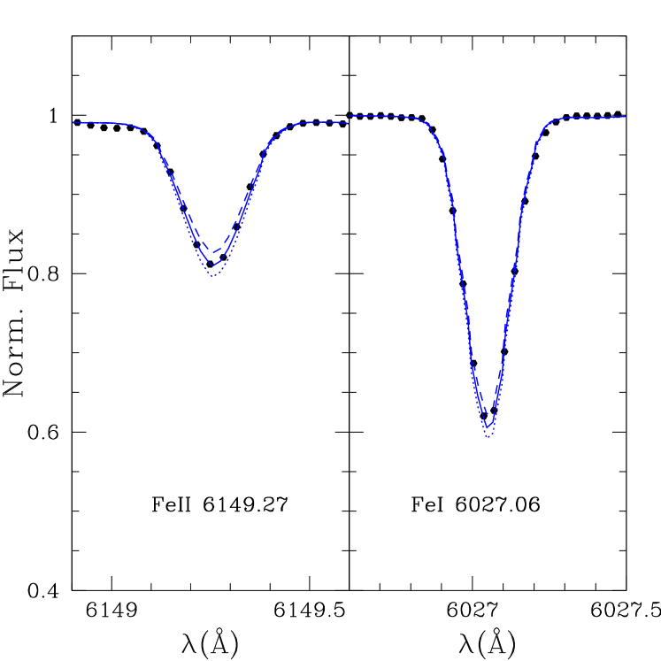
Figure 2: Fits of the observed spectra for HD 140901. The solid line is the fit corresponding to the derived $Z$ and the dotted and dashed lines are spectra computed for $+1\sigma$ and $-1\sigma$ from the average.

The first step of this procedure is to calibrate the atomic data list using the Kurucz’s solar spectrum and the corresponding solar atmosphere, which has $T_{\rm eff}=5777$ K, $\log g=4.437$ and $\xi=1.5\;{\rm km\;s^{-1}}$. For each selected line we changed the oscillator strength ($\log gf$) in the Kurucz’s atomic linelist until it reproduced the observed solar spectrum. In Table 9 we give the values of Ramírez et al. (2007), Reddy et al. (2003) and Affer et al. (2005), and the adopted values that we have used in our analysis. The equivalent widths of the fitted solar lines measured with the IRAF task splot are given as well. Therefore, the oscillator strengths will be fixed when fitting the spectra of the FGK stars that we have observed. After discerning which lines were suitable for the fitting procedure we selected the value of $\log g$ (3.5, 4.0 or 4.5) that gave the same abundances for different species and different ionization states. We estimated the value of the microturbulence, $\xi$, using the relationship derived by Allende Prieto et al. (2004) as function of $T_{\rm eff}$ and $\log g$ — see Table 10). After obtaining the metallicity considering the proper $\log g$ and $\xi$, we recalculated the $T_{\rm eff}$ performing again the corresponding fit to synthetic photometry, which led to negligible adjustments. Another parameter that could affect the determination of metallicity is the macroturbulence. We adjusted this parameter using a rotational profile and a Gaussian broadening function independently. Both approximations led to the same metallicities. In Fig. 2 we show the spectral fits for one of the companions of the DA white dwarfs (HD 140901). We have chosen to plot the fits corresponding to Fe i and Fe ii, to show how the method works for different ionization states.

4.3 Age determination

Table 10: Stellar parameters derived for the observed FGK stars.

Name	$T_{\rm eff}$	$\xi$	[Fe/H]	$Z$	$\log g$	$\log(L/L_{\sun})$	Isoch. Age
	(K)	(${\rm km\;s^{-1}}$)			(dex)		(Gyr)
G158$-$771,2	$4390\pm 30$	$...$	$...$	$...$	$...$	$...$	$...$
BD $-$01 469A3	$4480\pm 50$	$0.898$	$-0.10\pm 0.08$	$0.016\pm 0.003$	$3.5$	$1.669\pm 0.109$	$4.17^{+3.04}_{-2.05}$
HD 26965	$5140\pm 15$	$1.137$	$-0.41\pm 0.07$	$0.008\pm 0.001$	$4.5$	$-0.344\pm 0.094$	$...$
BD $+$44 1847	$5630\pm 50$	$1.305$	$-0.44\pm 0.05$	$0.007\pm 0.001$	$4.5$	$-0.184\pm 0.059$	$...$
BD $+$23 25391	$5665\pm 50$	$1.317$	$0.03\pm 0.06$	$0.021\pm 0.003$	$4.5$	$...$	$...$
BD $+$34 2473	$6270\pm 70$	$1.524$	$-0.12\pm 0.04$	$0.015\pm 0.002$	$4.5$	$0.379\pm 0.109$	$3.26^{+0.74}_{-1.46}$
HD 140901	$5635\pm 50$	$1.306$	$0.02\pm 0.07$	$0.021\pm 0.003$	$4.5$	$-0.055\pm 0.012$	$...$
HD 147513	$5985\pm 75$	$1.426$	$0.001\pm 0.077$	$0.020\pm 0.003$	$4.5$	$0.029\pm 0.017$	$...$
HD 1535804	$6470\pm 90$	$1.592$	$-0.01\pm 0.01$	$0.019\pm 0.004$	$4.5$	$0.671\pm 0.042$	$2.51^{+0.34}_{-0.32}$
BD $-$08 5980	$5670\pm 50$	$1.318$	$-0.37\pm 0.05$	$0.008\pm 0.001$	$4.5$	$-0.140\pm 0.040$	$...$

The distance of these stars is not known.
Low S/N.
[Fe/H] taken from McWilliam (1990).
[Fe/H] taken from Taylor (2003).

Table 11: X-ray parameters given by the ROSAT Catalog and the ages derived.

Name	$HR$	Count Rate	$\log(L_{x})$	Age
		(c/s)		(Gyr)
HD 26965	$-0.28\pm 0.06$	$0.796\pm 0.052$	$28.22\pm 0.12$	$1.07\pm 0.37$
HD 140901	$-0.73\pm 0.11$	$0.150\pm 0.023$	$28.27\pm 0.31$	$0.94\pm 0.50$
HD 147513	$-0.25\pm 0.06$	$0.650\pm 0.045$	$28.95\pm 0.14$	$0.33\pm 0.12$

Figure 3: Hertzsprung-Russell diagram for the companions. The isochrones of Schaller et al. (1992) for different ages (ZAMS, 2, 3 and 7 Gyr, from left to right) and solar metallicity are also plotted.

Figure 4: X-ray luminosity versus age for stars with different spectral types according to Ribas et al. (2007).

For most of our stars in our sample the parallax is known (from the Hipparcos Catalogue), thus, the calculation of the luminosity, $L$, is straightforward using the apparent magnitude after estimating the bolometric magnitude, $M_{\rm bol}$. For best accuracy we have used the $K$ band magnitude and the bolometric corrections of Masana et al. (2006). In Fig. 3 we show the Hertzsprung-Russell diagram for the FGK stars in our list with known distances. The isochrones of Schaller et al. (1992) for different ages and solar metallicity have been also plotted to show at which evolutionary state these stars are. As can be seen, the isochrone fitting technique is suitable for BD $+$34 2473, HD 153580 (both F stars) and for BD $-$01 469A (K subgiant). The rest of stars are too close to the ZAMS and hence the use of isochrones does not provide accurate values for their ages. When the isochrone fitting is appropriate, we have performed an interpolation in the grid of stellar models of Schaller et al. (1992) considering the derived $T_{\rm eff}$, $Z$ and $L$ to obtain the ages of these stars, i.e., the total ages of the white dwarfs in the common proper motion pairs. Our results are given in Table 10.

Another age indicator which could be used is X-ray luminosity. For some of these objects there are data available from the ROSAT All-Sky Bright Source Catalogue — 1RXS (Voges 1999) — which gives the count rate (number of detected counts per second) and the hardness ratio, $HR$. The hardness ratio is defined $HR=(H-S)/(H+S)$, where $H$ and $S$ are respectively the counts recorded in the hard and soft PSPC pulse height channels. To obtain the X-ray flux of a given star, we considered the calibrations of Schmitt et al. (1995). In particular, we used the conversion factor to obtain the energy flux from the measured count rate, which depends on $HR$:

$$CF=(5.30HR+8.31)\times 10^{-12}\;{\rm ergs}\;{\rm cm}^{-2}\;{\rm counts}^{-1}$$ (1)

Ribas et al. (2007) calculated a relationship between the age and X-ray luminosity for stars of different spectral types (Fig. 4) using both cluster data and stars belonging to wide binaries, or using kinematic criteria. In Table 11 we give the ROSAT information regarding these objects, the X-ray luminosity and the ages derived for the FGK companions with X-ray emission. The errors of the ages have been calculated considering the errors in the X-ray luminosity and an assumed cosmic dispersion for each relation (8 and 20% for G and K stars, respectively). There is also ROSAT information available for HD 153580, but since it is a member of a spectroscopic binary these relations cannot be applied.

Table 12: Ages, metallicities and masses for the white dwarfs in these common proper motion pairs.

WD	Age	$t_{\rm cool}$	$t_{\rm MS}$	$M_{\rm F}$	$M_{\rm I}$	$Z$
	(Gyr)	(Gyr)	(Gyr)	($\rm M_{\sun}$)	($\rm M_{\sun}$)
WD0315$-$011	$4.17^{+3.04}_{-2.05}$	$1.20\pm 0.56$	$2.97^{+3.09}_{-2.12}$	$0.60\pm 0.20$	$1.48^{+0.87}_{-0.28}$	$0.016\pm 0.003$
WD0413$-$017	$1.07\pm 0.37$	$0.112\pm 0.008$	$0.96\pm 0.37$	$0.54\pm 0.02$	$2.07^{+0.53}_{-0.27}$	$0.008\pm 0.001$
WD1354$+$340	$3.26^{+0.74}_{-1.46}$	$0.20\pm 0.02$	$3.06^{+0.74}_{-1.46}$	$0.50\pm 0.04$	$1.46^{+0.31}_{-0.09}$	$0.015\pm 0.002$
WD1544$-$377	$0.94\pm 0.50$	$0.76\pm 0.05$	$0.18\pm 0.50$	$0.78\pm 0.02$	$4.13^{+?}_{-1.49}$	$0.021\pm 0.003$
WD1620$-$391	$0.33\pm 0.12$	$0.026\pm 0.001$	$0.30\pm 0.12$	$0.63\pm 0.01$	$3.45^{+0.65}_{-0.35}$	$0.020\pm 0.003$
WD1659$-$531	$2.51^{+0.34}_{-0.32}$	$0.24\pm 0.01$	$2.27^{+0.34}_{-0.32}$	$0.66\pm 0.01$	$1.58^{+0.08}_{-0.05}$	$0.019\pm 0.004$

5 The initial-final mass relationship

Figure 5: Final masses versus initial masses for the common proper motion pairs studied here and some precise available data.

Once we know the total age of the white dwarfs and the metallicity of their progenitors, the initial masses can be derived considering suitable stellar models. In our case we have used the stellar tracks of Domínguez et al. (1999). The initial and final masses obtained are detailed in Table 12. Other parameters, such as overall ages, cooling times, main-sequence lifetimes of the progenitors and metallicities are also given. As can be noted all the total ages exceed the cooling times, as expected.

In Fig. 5 we represent the final masses versus the initial masses obtained for the white dwarfs in our sample for which the age and metallicity have been derived. The lines correspond to the theoretical initial-final mass relationships of Domínguez et al. (1999) for different metallicities. For the sake of comparison we have also included the most precise data that are currently being used to define the semi-empirical initial-final mass relationship. For the Hyades and Praesepe, we plot the results obtained by Claver et al. (2001), and some recent results from Dobbie et al. (2004, 2006). We also used the results of Dobbie et al. (2006) for the only known Pleiades white dwarf. In the case of Sirius, we have used the initial and final masses derived by Liebert et al. (2005b).

From an inspection of Fig. 5 it can be noted that the observational data present large dispersion, which is higher than the uncertainties, in comparison with the theoretical initial-final mass relationships of Domínguez et al. (1999). According to our results, a main-sequence star of $1.5\,\rm M_{\sun}$ with approximately solar metallicity could end up as white dwarfs with masses that differ by $\sim 25\%$ (cf. WD1354$+$340 and WD1659$-$531). Moreover, two white dwarfs of nearly the same masses could come from main-sequence stars with masses different by a factor of 2 (cf. WD1620$-$391 and WD1659$-$531). Apparently, this difference is not a consequence of metallicity, since it is practically the same for these objects (Table 12). However, it is also interesting to note that the influence of metallicity on the theoretical initial-final mass relationship seems to be almost negligible below $2\,\rm M_{\sun}$. Other factors, such as magnetic fields or rotation (Domínguez et al. 1996) should be studied in detail in order to discern their effect on this relation.

The ages of star clusters are usually calculated to a higher accuracy than in the case of the individual low-mass stars considered in this work, which should allow to obtain the initial masses with better accuracy. However, from Fig. 5 it can be noted that white dwarfs in clusters display a large dispersion, especially between $3$ and $4\,\rm M_{\sun}$. Thus, this scatter in the observational data seems to be a real effect, rather than a consequence of the uncertainties in the mass estimates. Hence, there is no apparent reason for which the initial-final mass relationship should be considered a single-valued function. A thorough complete comparison of our results based in common proper motion pairs with cluster data will be discussed in a forthcoming paper (Catalán et al. 2008).

One of the most important contributions of our work is the study of the range of initial masses corresponding to $1.5-2\,\rm M_{\sun}$, which was not covered by the research based on open cluster data (Ferrario et al. 2005, Dobbie et al. 2006). The recent study of Kalirai et al. (2007) using old open clusters has also provided some new data in the low-mass domain. It is worth to mention that 5 of the 6 white dwarfs of our final sample have masses near the typical values derived by, e.g., Kepler et al. (2007), $M\sim 0.6\,\rm M_{\sun}$, which represent 90% of the white dwarfs found in the SDSS. This stems from the fact that the progenitors of white dwarfs in open clusters were usually more massive ($M>2\,\rm M_{\sun}$) since clusters are relatively young and the low-mass stars, which would produce the typical white dwarfs, are still on the main sequence. Since some of the pairs that we have studied have larger ages than the typical values for open clusters, the white dwarfs that belong to these pairs can be less massive. Thus, we consider that white dwarfs in common proper motion pairs are more representative of the Galactic white dwarf field population than white dwarfs in open clusters.

6 Summary and Conclusions

We have studied a sample of common proper motion pairs comprised of a white dwarf and a FGK star. We have performed high signal-to-noise low resolution spectroscopy of the white dwarf members, which led us to carry out a full analysis of their spectra and to make a re-classification when necessary. From the fit of their spectra to white dwarf models we have derived their atmospheric parameters. Then, using different cooling sequences — namely those of Salaris et al. (2000) and Fontaine et al. (2001) — their masses and cooling times were obtained. Simultaneously, we have performed independent high resolution spectroscopic observations of their companions. Using the available photometry we have obtained their effective temperatures. Then, from a detailed analysis of their spectra and using either isochrones or X-ray luminosities, we have derived their metallicities and ages (i.e., the metallicities of the progenitors of the white dwarfs and their total ages).

These observations allowed us to obtain the initial and final masses of six white dwarfs in common proper motion pairs, four of them corresponding to initial masses below $2\,\rm M_{\sun}$, a range which has not been previously covered by the open cluster data. Our semi-empirical relation shows significant scatter, compatible with the results obtained by Ferrario et al. (2005) and Dobbie et al. (2006), which are mainly based on open cluster data. However, the dispersion of the results is higher than the error bars, which leaves some open questions that should be studied in detail (e.g., rotation or magnetic fields).

We have shown that common proper motion pairs containing white dwarfs can be useful to improve the initial-final mass relationship, since they cover a wide range of ages, masses and metallicities, and they are also representative of the disk white dwarf population. We have seen that the accuracy in the total ages depends almost exclusively on the evolutionary state of the low-mass companions. Such relative accuracy becomes poor when the star is close to the ZAMS. However, this limitation may not be critical to many common proper motion pairs. Planned deep surveys like GAIA, LSST or the Alhambra Survey will discover thousands of new white dwarfs, some of them belonging to wide binaries. In the meantime, our most immediate priority is to further extend the sample of wide binaries valid for this study. We are working in the search for more wide binaries of our interest in the NLTT catalog (Gould & Chanamé 2004) and also in the LSPM-north catalog (Lépine & Bongiorno 2007). Detailed study of the current and future common proper motion pairs of this type should help to explain the scatter in the semi-empirical initial-final mass relationship and to discern whether this is a single-valued function. If consistency between observations and theoretical calculations is found, this would have a strong impact on stellar astrophysics, since this relationship is used in many different areas, such as chemical evolution of galaxies, the determination of supernova rates or star formation and feedback processes in galaxies.