Lattice QCD with two light Wilson quarks and maximally twisted mass
Abstract:
We summarise status and recent results of the European Twisted Mass collaboration (ETMC). The collaboration has been generating gauge configurations for three different values of the lattice spacing and values of the charged pseudo scalar mass as low as with two flavours of maximally twisted mass quarks. We provide evidence that improvement works very well with maximally twisted mass fermions and that also higher order lattice artifacts appear to be small. The currently only quantity in the light meson and baryon sector where cut-off effects are visible is the neutral pseudo scalar mass and we present an attempt to understand this from a theoretical point of view.
We describe finite size effects and quark mass dependence of the mass and decay constant of the (charged) pseudo scalar meson with chiral perturbation theory formulae and our current estimate for the low energy constants is and . Results for the average up-down, the strange and the charm quark mass and the chiral condensate are also presented.
1 Introduction
Whenever results obtained from lattice QCD simulations are to be confronted with experimental results it is important to have a sound control of systematic uncertainties emerging in lattice QCD. The most prominent of those are discretisation errors, finite size effects (FSE) and uncertainties arising from the unphysically large mass values usually simulated. The main reason for their prominence is the fact that lattice QCD simulations become increasingly computer time demanding when a) the lattice spacing is reduced b) the quark masses are reduced towards the physical point and c) the volume is increased.
The control of these systematic uncertainties requires simulations with an improved lattice formulation at sufficiently small values of the lattice spacing , say where lattice artifacts are small. Physical volumes should be large enough, say with spatial box size larger than and ( is the mass of the lightest pseudo scalar particle). And, in order to be able to utilise chiral perturbation theory (PT) to bridge between simulated quark masses and the physical point, simulations with a range of masses are needed, with the smallest value of . It goes without saying that the aforementioned bounds are only estimates and need to be checked carefully in actual simulations.
Due to recent algorithmic improvements [1, 2, 3, 4, 5, 6] it became possible to meet all these requirements using Wilson’s original formulation of lattice QCD. It has the advantage of being conceptually clear and simple. And, improvement can be implemented in several ways, one of which is using so called Wilson twisted mass fermions [7] at maximal twist. As was shown in Ref.[8], in maximally twisted mass lattice QCD (Mtm-LQCD) physical observables can be obtained improved by tuning a single parameter only. In particular, no operator specific improvement coefficients need to be computed. This theoretical expectation could be verified in the quenched approximation to work very well [9, 10, 11, 12] (for a recent review see Ref. [13].)
Based on these successes in the quenched approximation the European Twisted Mass (ETM) collaboration decided to start a large scale simulation project using two flavours of mass degenerate quarks with the lattice formulation of Mtm-LQCD. First accounts of this effort are published in Refs. [14, 15, 16] indicating that improvement works very well when sea quark effects are taken into account in the simulations. This proceeding contribution aims to summarise the progress and current status of the two flavour project of the ETM collaboration.
2 Gauge and Fermionic Action
In the gauge sector we employ the so-called tree-level Symanzik improved gauge action (tlSym) [17], viz.
with the bare inverse gauge coupling , and . The fermionic action for two flavours of maximally twisted, mass degenerate quarks in the so called twisted basis [7, 8] reads
| (1) |
where is the untwisted bare quark mass, is the bare twisted quark mass, is the third Pauli matrix acting in flavour space and
is the mass-less Wilson-Dirac operator. and are the forward and backward covariant difference operators, respectively. Twisted mass fermions are said to be at maximal twist if the bare untwisted mass is tuned to its critical value , the situation we shall be interested in. For convenience we define the hopping parameter . Note that we shall use the twisted basis throughout this paper.
Maximally twisted mass fermions share most of their properties with Wilson’s originally proposed formulation, but provide important advantages: the spectrum of is bounded from below, which was the original reason to consider twisted mass fermions. The twisted mass is related directly to the physical quark mass and renormalises multiplicatively only. Many mixings under renormalisation are greatly simplified. And – most importantly – as was first shown in Ref. [8] physical observables are automatically improved without the need to determine any operator-specific improvement coefficients.
The main drawback of maximally twisted mass fermions is that flavour symmetry is broken explicitly at finite value of the lattice spacing, which amounts to effects in physical observables. However, it turns out that this is presumably only relevant for the mass of the neutral pseudo scalar meson (and closely related quantities). We shall discuss this issue in more detail later on.
2.1 Improvement in Practice
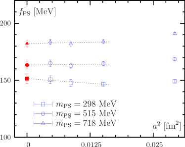
It is well established in the literature that improvement works very well in practice in the quenched approximation [9, 10, 11, 18, 19, 12]. As an example we show in figure 1(a) the essentially flat continuum extrapolation in of the pseudo scalar decay constant in physical units ( was used to set the scale) for three reference values of the pseudo scalar mass as obtained in Ref. [11].
So far we did not discuss how maximal twist can be achieved in practise and there are various solutions to this problem. Emerging from the proof of improvement at maximal twist [20, 21] the general prescription is to choose a parity odd operator and determine such that has vanishing expectation value at fixed physical situation for all lattice spacings. The physical situation can be fixed for instance by keeping in physical units fixed, where is the mass of the lightest charged pseudo scalar particle. One possible quantity to tune is the PCAC quark mass, defined as
| (2) |
where and are the axial vector current and the pseudo scalar density, respectively,
Tuning the PCAC mass to zero has been successful in the context of the aforementioned quenched investigations, in agreement with theoretical considerations [22, 23, 20]. The collaboration follows the strategy to determine the value of at the lowest available value of , which is sufficient to guarantee improvement [20].
3 Setup and Tuning
In table 1 we summarise the various ensembles produced by the ETM collaboration. We have simulations for three different values of the inverse gauge coupling , and . The corresponding values of the lattice spacing are about , and , respectively (see later). For each value of we have four or five different values of the bare twisted mass parameter , chosen such that the simulations cover a range of pseudo scalar masses between and .
The physical box sizes of the simulations at and are roughly equal and around , while the volume at is slightly larger. For all -values we have carried out simulations at different physical volumes in order to check for finite size (FS) effects. For each value of and (ensemble) we have produced around equilibrated trajectories in units of . The actual trajectory length is given in table 1. In all cases we allowed for at least trajectories for equilibration (again in units of ).
Note that the analyses for the ensembles at are in a very preliminary status for reasons that will be explained later. For the purpose of this proceeding contribution results are excluded from most of the present analyses.
| Ensemble | |||||||
|---|---|---|---|---|---|---|---|
The determination of for instance quark masses requires a renormalisation procedure. To this end we have implemented the non-perturbative RI-MOM renormalisation scheme [24], which provides in the case of maximally twisted mass fermions improved renormalisation constants [25]. Where appropriate, we convert our results to the scheme at the desired scale using renormalisation group improved continuum perturbation theory at N3LO [26]. For details on this procedure we refer to Ref. [25, 27].
3.1 Algorithm Stability and Performance
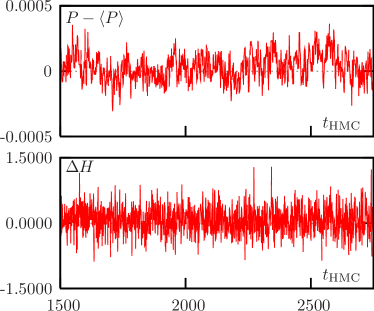
The algorithm we used is a HMC algorithm [28] with mass preconditioning [1, 29] and multiple time scale integration (mtmHMC), as described in detail in Refs. [5, 30]. The algorithm performs smoothly and without any instabilities in the whole range of simulation parameters we have available. In particular we do not observe any instabilities at our smallest values for the twisted mass parameter for the different values of . In figure 1(b) we illustrate this with the Monte Carlo history of the plaquette and the difference in the HMC Hamiltonian for ensemble . For further details about the algorithmic parameters used see Ref. [31].
Due to the fact that the twisted mass parameter provides an infra-red cut-off for the eigenvalue spectrum of the lattice Dirac operator we do not expect instabilities due to very small or zero eigenvalues (for a discussion of this issue for Wilson fermions see Ref. [32]). However, Wilson type fermions exhibit a non-trivial phase structure at finite value of the lattice spacing with a first order phase transition at the chiral point for our choice of the gauge and fermionic action [33, 34, 35, 36, 37, 38]. As a consequence simulations at given, finite value of the lattice spacing cannot be performed with arbitrarily small values of the bare quark mass and one needs to make sure that the values of the twisted mass parameter are large enough for the simulations not to be affected by the first order phase transition.
This issue was thoroughly investigated by the ETM collaboration with the result that we do not see metastabilities for any of our simulation points. But, as a matter of fact, simulations at large value of the lattice spacing and maximal twist are performed potentially in the close vicinity of the (second order) critical endpoint at of the first order phase transition line. This line extends in the --parameter plane to a first approximation perpendicular to the -axis from to (see Ref. [13] and references therein for a more detailed discussion). Hence, there is the danger for long autocorrelation times in quantities that are not continuous at the phase transition like for instance the plaquette or the PCAC quark mass .
This is supported by table 1 where we give estimates of the integrated autocorrelation times for the plaquette and the pseudo scalar mass. While for the pseudo scalar mass is always moderately small and depending only weakly on the values of and , this is not the case for the plaquette: there is a trend in the data that decreases with increasing values of and , even though the statistical errors are so large that the -dependence is not significant. Note that the -values for are similar to those for the plaquette. Fortunately, we observe very long autocorrelation times only for our smallest -value. This is the reason that we are still investigating the error analysis for those ensembles. This affects the determination of the PCAC quark mass, which is needed to tune to maximal twist. Hence, at this stage, we use the corresponding results at only for estimating systematic errors.
In order to investigate algorithm stability it was suggested in Ref. [39] to study the statistical distribution of the twist angle as a function of the quark mass. The quantity of interest is the PCAC quark mass, evaluated in the background of a given gauge configuration by taking the axial to pseudo scalar correlator at some large value for normalised by . Here is the pseudo scalar correlator averaged over all gauges evaluated at the same value of . The PCAC quark mass is related to the twist angle by
The statistical distribution of resembles always to a very good approximation a normal distribution. As will be discussed later, at fixed value of and the distribution mean depends on as expected. For all three -values the standard deviation is increasing at the order of a few percent with increasing . In addition we observe a smooth dependence of the standard deviation on and the lattice spacing. Hence, there is no sign for instabilities seen in .
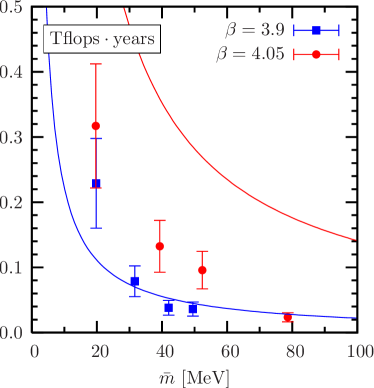
It is interesting to compare the performance of our HMC variant with the one using domain decomposition as a preconditioner (DD-HMC) (instead of mass preconditioning), which is described in Ref. [40]. A useful performance figure is the number of floating point operations required to generate independent gauge configurations as a function of the box size , the lattice spacing and the quark mass in the scheme at [41, 42]
| (3) |
In Ref. [42] the parameters in Eq. (3) for the DD-HMC algorithm with Wilson fermions are estimated roughly to , , and , which is a significant improvement as compared to cost estimates for the original HMC algorithm, see for instance Ref. [41]. Using the integrated autocorrelation time of the plaquette as a measure for the autocorrelation of two gauge configurations we can measure for the mtmHMC algorithm and compare the result in figure 2(a) to the cost estimate for the DD-HMC algorithm [42].
Figure 2(a) reveals that the performance of the two algorithms is very similar. In particular for the larger value of the two plotted lattice spacings the agreement is rather good. For our HMC version the lattice spacing dependence appears to be milder. However, one should keep in mind the large errors associated to this cost figure. Moreover, the result may depend significantly on how much effort is invested into tuning of algorithmic parameters.
3.2 Sommer Parameter
In order to be able to compare results at different values of the lattice spacing it is convenient to measure the hadronic scale [43]. It is defined via the force between static quarks at intermediate distance and can be measured to high accuracy in lattice QCD simulations. For details on how we measure we refer to Ref. [31].
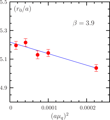
In figure 2(b) we show as a function of for . The mass dependence appears to be rather weak and a quadratic fit in to our data describes the data rather well. The results we obtain for the three -values in the chiral limit are at , at and at . The statistical accuracy for is about . Note that the data is also compatible with a linear dependence on and a linear fit gives consistent results in the chiral limit.
3.3 Tuning to Maximal Twist
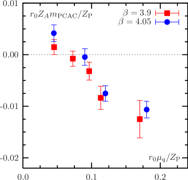
In order to obtain improvement the bare quark mass must be tuned to its critical value. As mentioned before we use the PCAC quark mass defined in Eq. (2) for tuning to maximal twist. The goal was to tune this quantity to zero approximately at the smallest available -value at each lattice spacing, which corresponds to approximately fixed physical pseudo scalar mass. Considering only and , it was possible to perform this tuning task with two or three tuning runs for each lattice spacing.
The result is plotted in figure 3(a), where we plot the renormalised against the renormalised , both in units of , for and . The renormalisation factors were determined using the RI-MOM scheme. Within the statistical accuracy the PCAC quark mass is zero at a common value of the renormalised twisted mass. For all other values of we observe (small) deviations from zero. This dependence is an cut-off effect which will modify only the lattice artifacts of physical observables. The numerical precision we were aiming for was , where is the uncertainty on the PCAC quark mass at the lowest value of [44]. It turns out that the accuracy we have achieved is sufficient for excellent scaling properties, as will be seen later.
4 Results
The ETM collaboration is currently analysing the generated gauge configurations for many different observables. Not all of these – partly preliminary – results can be summarised here and we shall therefore mainly concentrate on the pseudo scalar sector. At the end of this section we present an overview of the available results and give references of the corresponding proceedings contributions.
4.1 Charged Pseudo Scalar Mass and Decay Constant
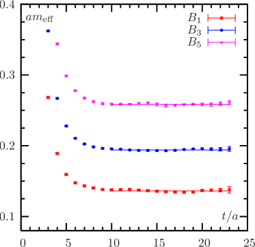
The charged pseudo scalar meson mass can be extracted from the time exponential decay of suitable correlation functions. For details on our analysis procedure see Ref. [31]. To demonstrate the quality of our data we show in figure 3(b) effective mass plots for the ensembles , and obtained from the pseudo scalar correlation function. The final values for the masses are obtained from a fit to a matrix of correlators [31]. We also attempted to determine the energy of the first excited state of the pseudo scalar meson. We were not able to determine it with any reliability from an unconstrained fit. (In particular, there is no evidence for an excited state with mass , which is theoretically possible for maximally twisted mass fermions [13].) Constraining the energy of the first excited state to three times the ground state mass, however, does allow for an acceptable fit.
For maximally twisted mass fermions the charged pseudo scalar decay constant can be extracted from
| (4) |
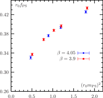
due to the exact lattice PCVC relation with no need to compute any renormalisation constant [7]. Thanks to this advantage and having the results for at hand we plot the results for as a function of for and in figure 4(a). We plot only the results for the ensembles to and to in order to have approximately equal physical volumes for the two values of . Figure 4(a) provides first evidence that lattice artifacts in those two quantities are small.
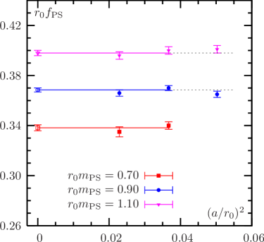
Continuum Extrapolation of at Fixed Volume
This statement can be brought to a more quantitative level for instance for the pseudo scalar decay constant. To this end we interpolate at every lattice spacing linearly in to fixed values of . We corrected for the very small difference in the physical volume [44].
The interpolated data points are plotted in figure 4(b) for three values of , and as functions of . It is visible that the differences between the data at and are of the order of the statistical accuracy and hence, we perform a weighted average of these two lattice spacings to obtain continuum estimates. This indicates again that scaling violations are very small in the pseudo scalar decay constant.
Even though we are still investigating the error analysis we plot in figure 4(b) also the results for for those reference points where we are able to interpolate to the reference values of (for the lowest value of we currently need to extrapolate). Keeping in mind that these data points are very preliminary we can nevertheless say that they fit rather well into the picture that lattice artifacts are very small.
Other quantities – for instance the renormalised quark mass – show a similar scaling behaviour as discussed in Ref. [44], where also the results at are discussed in more detail.
Finite Size Effects
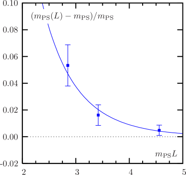
At the level of statistical accuracy we have achieved now, finite size effects for and cannot be neglected. It is therefore of importance to study whether the FS effects can be described within the framework of chiral perturbation theory. This requires to compare simulations with different lattice volumes and all other parameters kept fixed, like for instance ensembles , and or and . For all these ensembles holds, which is believed to be needed for PT formulae to apply. The first observation we make is that the finite size effects are compatible with an exponential behaviour in . As an example we plot in figure 5(a) the relative finite size effects
| (5) |
for against . The value of was obtained by fitting the chiral perturbation theory inspired formula
| (6) |
to our data, with and being free parameters [45]. A similar fit can be performed for by using the value of as obtained from the first fit as input. Both fits describe the data rather well with .
| Ensemble | |||||
|---|---|---|---|---|---|
We shall now compare the measured finite size effects to predictions of continuum chiral perturbation theory (PT) (lattice artifacts appear to be negligible, as discussed before). The comparison reveals that continuum PT formulae can describe FS effects within our statistical accuracy.
The NLO PT formulae for and were derived in Ref. [46] (for short GL) and can be written as
| (7) |
where
| (8) |
is a known function [46] and the finite size corrections depend apart from and only on the unknown leading order low energy constant (note that our normalisation is such that ). For the pseudo scalar meson mass the corrections are also known to two loops [47], but the asymptotic Lüscher formula [48, 49] (for short CDH) provides an easier way to access higher order corrections to and , and the differences to the NNLO formula turn out to be small [47]. The drawback of CDH compared to GL is that additional parameters are needed as an input, among others the low energy constants , , and . Since we do not have enough data points to determine all these parameters from a fit to only FS data we have to rely on estimates available in the literature [49].
Assuming that the results for the ensembles and provide the infinite volume estimates for and , we can compute the relative FS effects using Eq. (5) for the ensembles , and , which we denote with . These measured estimates can then be compared to the PT predictions computed with the formulae from GL and CDH, denoted by and , respectively. The values of the unknown low energy constants are set to the estimates provided in Ref. [49]. In order to do so and for evaluating the CDH formulae we need the value of the lattice spacing which we estimate using .
The results for , and are compiled in table 2. It turns out that – in particular for – the asymptotic formula from CDH describes the data better than the one loop formula from GL: the CDH corrected data is in agreement with the infinite volume estimate within the statistical accuracy. Note that the observation that GL usually strongly underestimates the FS effects in can also be made from the Wilson data published in Ref. [50] (cf. Ref. [39]).
These results make us confident that our simulations have eventually reached a regime of pseudo scalar masses and lattice volumes where PT formulae can be used to estimate FS effects. But it is clear that in particular the CDH formula is affected by large uncertainties, mainly stemming from the only poorly known low energy constants, which are needed as input. Changing their values in the range suggested in Ref. [49], however, changes the estimated finite size effects maximally at the order of about (of the corrections themselves).
Quark Mass Dependence and Chiral Perturbation Theory
So far we have argued that lattice artifacts in charged and for and are very small and that FS effects can be described using PT formulae. We shall now show that also the quark mass dependence of these quantities can be successfully described using PT. This will in addition allow the determination of most of the aforementioned low energy constants and the lattice scale.
As chiral symmetry is broken by the lattice Wilson term, eventually the chiral extrapolation should be done using continuum extrapolated, infinite volume data. This is described for our data in Ref. [44]. However, since lattice artifacts are not visible with our current statistical accuracy of about (and chiral symmetry breaking as well as flavour symmetry breaking are formally lattice artifacts of ), we can follow a different approach.
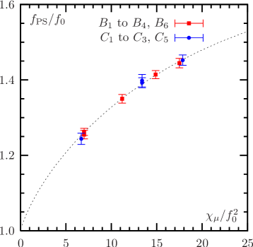
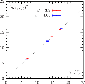
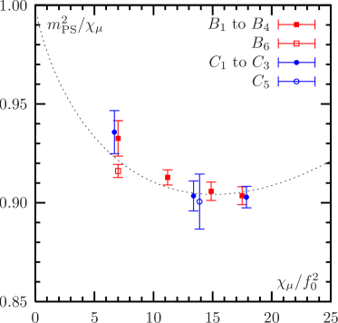
This approach consists of describing our data for and at and simultaneously with continuum chiral perturbation theory. We fit the appropriate () continuum NLO PT formulae [46, 49]
| (9) |
| (10) |
to our raw data for and simultaneously for and . parametrise the FS corrections for which we can either use the GL or the CDH formulae. Both and depend on low energy constants as well as on and . The notation is
| (11) |
and the normalisation , i.e. . In Eqs. (9) and (10) NNLO PT corrections are assumed to be negligible. This approach has the advantage that we can include finite size data consistently in the fit and that we can use more raw data points. In addition we do not need to interpolate our data to reference points. The fit presented in the following is an extension to the fit presented for only in Ref. [16].
The fit can be parametrised by six free parameters: two dimensionless ratios and and in lattice units for both -values, i.e. , , , , and .
Finite size effects are corrected for by using the asymptotic formulae from CDH, which is consistently included in the fit. The parameters that are not fitted, basically and , are set to the values suggested in Ref. [49]. Also the lattice spacing in , needed for evaluating the CDH formula, can be determined consistently from the fit by setting where the ratio assumes its physical value. Note that in this ratio we use the physical value of the neutral pseudo scalar meson mass, in order to account for electro magnetic effects not present in the lattice simulation.
The ensembles we use in the fit are to and to . In addition we include the ensembles and in the fit in order to explore the dependence of our data. We do not use in order not to give too much weight to this -value. The ensembles and , the largest available masses, are not included in the fit, because they lead to significantly increased in the fit and hence we conclude that NLO PT is not appropriate for such large mass-values.
Our data for and is described excellently by the PT formulae, see figures 5(b), 6(a) and 6(b), where we plot appropriate, dimensionless ratios. The fitted values of the parameters are
| (12) |
with and statistical errors only. The sensitivity to is visualised by the deviation from linearity in figures 5(b) and 6(b).
The statistical uncertainties are estimated using a bootstrap procedure: at each of our data points we produced bootstrap samples of and and used them to perform fits. The statistical uncertainty is then given by the variance over these fit results. Note that this procedure automatically takes into account the cross-correlation between and for a given ensemble.
Systematic uncertainties are – as usual – harder to estimate. We include the effects coming from (a) finite size effects by using GL instead of CDH to estimate finite volume effects, (b) finite size effects by including and as free parameters in the fit and (c) lattice artifacts by performing the fits separately for and . They are discussed in more detail in Ref. [44].
Lattice Calibration and Low Energy Constants
As mentioned above, by fixing the value of to the physical value of the pion decay constant where assumes its physical value we can calibrate our lattices for the two -values, with the result
| (13) |
The ratio can be compared with the ratio and we find excellent agreement. Moreover, using those values for the lattice spacings we can get an estimate of the ratio from our fit and compare it to the corresponding ratio as determined with RI-MOM. Also here the agreement is excellent. We take this as an indication that the combined fit does not hide lattice artifacts in fit parameters.
Having set the scale allows us to determine the low energy constants
| (14) |
where we set conventionally. The first error is statistical, the second systematical (see Ref. [44] for details on how we estimate the systematic errors). The statistical accuracy on these estimates for is quite impressive and the mean values are in good agreement with the literature (see Refs. [51, 52] for recent reviews).
4.2 Nucleon Mass
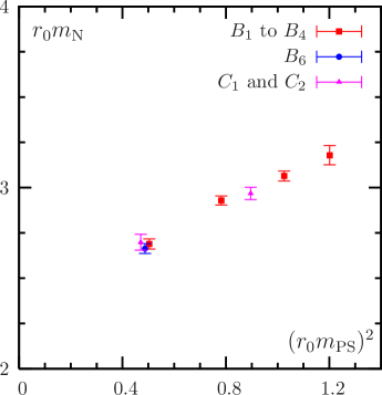
In figure 7(a) we plot our preliminary results for the nucleon mass in units of as a function of . Also in this quantity scaling violations are not visible within the statistical accuracy. Moreover, as shown by the comparison of ensemble and , finite size effects seem to be negligible. Concentrating on only, since we do not yet have enough data points at , we fit the leading one-loop Heavy Baryon PT formula [53, 54]
| (15) |
with and the two free parameters and to our data. The fit provides a good description of the data with . With the physical nucleon mass as input the value of the lattice spacing at can be determined to in very good agreement with the determination from . This result not only successfully cross checks the determination of the lattice spacing in physical units from . If confirmed, it also represents a test of QCD as the theory of strong interactions. For more details, including the error determination and other baryon masses see Ref. [55].
4.3 Flavour Symmetry Breaking Effects
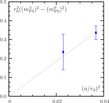
As mentioned in section 2, flavour symmetry is explicitly broken. As a consequence there is a potential difference of between the masses of charged and neutral pseudo scalar mesons. Notice that to the latter also disconnected diagrams contribute. We have determined the mass of the neutral pseudo scalar meson for the ensembles , , , and . The results are shown in table 3 where we also report the the corresponding values for the charged meson mass.
The neutral pseudo scalar meson is lighter than the charged one. This observation is consistent with PT predictions for the observed first order phase transition scenario (see Ref. [13] and references therein). For ensembles and we plot in figure 7(b) the difference
| (16) |
as a function of . The quantity (16) is expected to scale linearly in towards the continuum, which is confirmed by our data. The dashed line in figure 7(b) is not a fit, but it is there only to guide the eye.
Even if this analysis provides evidence for the expected scaling behaviour of the pion mass splitting, the effect still amounts to about at our smallest value of the lattice spacing and charged . If compared to the “natural” size one would expect for cut-off effects, which is of the order of , one has to conclude that this effect is unexpectedly large and one would like to be able to better understand it. Of particular interest is the question whether this effect arises dynamically, or is due to large coefficients in the Symanzik expansion. In the latter case one might expect that this effect is not restricted to only the neutral pseudo scalar meson mass.
Note that all other possible splittings we have determined so far are negligible. For instance the splittings in the vector and channels appear to be consistent with zero (see table 3 for and Ref. [55] for the ). Similarly, the difference between the decay constants of charged and neutral pseudo scalar meson is negligible.
Currently, the ETM collaboration is investigating this question [56, 57], and from a theoretical point of view, an analysis à la Symanzik of the charged and the neutral pseudo scalar meson masses lead to the formulae
| (17) |
which show that the difference is given by the term proportional to . Here and is the dimension six term in the Symanzik effective Lagrangian.
| Ensemble | ||||
|---|---|---|---|---|
The main result of the analysis of Refs. [56, 57] is that is a large number which in the vacuum saturation approximation can be estimated to be proportional to , where . The latter matrix element is numerically large: one finds around [56, 57]. This result can provide an interesting physical explanation for the large splitting observed in the pseudo scalar masses. Moreover, since it can be shown that enters only the neutral pseudo scalar mass (and related quantities), one also finds a possible explanation of why all other splittings determined so far turn out to be small. In addition it provides hope that in the future we shall not find large lattice artifacts due to flavour breaking.
At this point the question might arise whether the large splitting in the pseudo scalar masses affects the PT fits and in particular the PT FS estimates. At the current level of our analysis, where we work under the assumption that lattice artifacts are zero in charged and – and we have shown good theoretical and numerical evidence for this – all the fits are performed in the continuum, where flavour symmetry is restored. Hence, we do not expect any effect of flavour symmetry breaking on our analysis with PT.
4.4 Further ETMC Results
Our current simulations contain two light quark flavours with degenerate mass in the sea. In the unitary set-up we can hence determine the average up-down quark mass in the scheme by using PT fits discussed in section 4.1. The result is . We have again used the estimate for coming from RI-MOM [58, 25]. Here and in the following the first error is statistical, the second systematical.
In order to also determine the strange and possibly the charm quark masses, we have to use a partially quenched set-up where we compute propagators on the available gauge configurations with several values of the valence quark mass – which are now different from the sea quark mass – around the strange and the charm quark mass. The set-up and the calculation are described in detail in Refs. [59, 58] and the result for the strange quark mass for only reads . A comparison to other lattice QCD determinations of shows that non-perturbative renormalisation has significant impact on the final result. Estimates obtained with perturbative renormalisation tend to be significantly lower than estimates with non-perturbatively computed renormalisation constants. For more details as well as for further related results, such as the kaon decay constant and the ratio , we refer to Ref. [59, 58].
In Ref. [60] we present our current estimates for the charm quark mass at . Our result reads . In Ref. [60] also results for and are presented, which are in good agreement with experiment.
In addition, the gauge configurations at have been used to calculate a variety of 3-point correlation functions relevant for semileptonic weak decays and electromagnetic transitions of light and heavy-light pseudo scalar mesons. Results for the the vector, scalar and tensor form factors of the pion, the vector and scalar form factors relevant for Kl3 decay and for the Isgur-Wise function in the heavy-quark limit can be found in Ref. [61]. On the same set of gauge configurations there are preliminary results for the first moment of the pion quark distribution function available. They can be found in [62] together with an effective stochastic method to determine this quantity in lattice simulations.
The ETM collaboration has made a serious attempt to determine properties of flavour singlet mesons with Mtm-LQCD, a first account of which can be found in Ref. [63]. The most interesting result of this investigation is that the mass of the meson (the one related to the anomaly in two flavour QCD, i.e. not a Goldstone boson) is consistent with a constant behaviour in the chiral limit and the value around is compatible with expectations from a model computation [64]. (See also Ref. [65])
For certain quantities, like , it is crucial that the lattice formulation exhibits good chiral properties. The overlap operator, which obeys exact chiral symmetry at finite value of the lattice spacing, can be used in a mixed action approach as a valence operator on a maximally twisted mass sea. An exploratory study and first results profiting from the chiral properties in the valence sector can be found in Ref. [66].
A systematic uncertainty we cannot control at the moment is due to the fact that the effects of the strange quark are not taken into account in the simulations. In order to include these effects in Mtm-LQCD, maintaining improvement at the same time, a split heavy doublet of quarks has to be simulated in addition to the mass degenerate light quark doublet [67]. In an exploratory study, published in Ref. [68], it was shown that this approach is feasible and that tuning is possible. However, it was also shown that the effect of the first order phase transition, mentioned in previous sections, strengthens significantly when the heavy doublet is added. In Ref. [69] we report on an attempt to cure this potential problem by using stout smearing [70]. Our preliminary results suggest that stout smearing reduces indeed the effects of the phase transition significantly.
An interesting investigation at tree level of perturbation theory is presented in Ref. [71]. In this framework cut-off effects can be studied using analytic calculations. Scaling properties of Wilson and Wilson twisted mass fermions are compared and it is shown that maximally twisted mass fermions scale with a rate of .
For a study using Mtm-LQCD for simulations of QCD thermodynamics see Ref. [72].
4.5 Exploring the -regime with Maximally Twisted Mass Fermions
A slightly different direction as compared to all the aforementioned results is explored by performing studies of the -regime [73] with Mtm-LQCD at [74]. Simulations in the -regime are not restricted to formulations with exact chiral symmetry. And, since the twisted mass parameter provides – as discussed before – an infra-red cut-off to the eigenvalue spectrum of the twisted mass Dirac operator there is also no technical complication to expect, unlike that arises e.g. for Wilson fermions when the quark mass becomes too small.
Preliminary results of this investigation presented in Ref. [74] are quite encouraging. Simulations turn out to be feasible, perform smoothly and are much less computer time demanding than simulations with e.g. the overlap operator. A first result of this study at is an estimate for the chiral condensate , which is in perfect agreement with the value determined from the PT fit .
5 Summary
In this proceeding contribution we have summarised the current status of the two flavour project of the European Twisted Mass collaboration. The collaboration has generated gauge configurations using a doublet of mass degenerate Wilson twisted mass fermions at maximal twist for three different values of the lattice spacing , volumes with physical extent larger than and values for the (charged) pseudo scalar meson mass in the range of to . The results for the two finer lattice spacings of about and are close to final, while the results for the coarsest lattice spacing are still in a preliminary state.
We have presented results for (charged) and and a scaling analysis for at fixed, but finite volume indicating that improvement in Mtm-LQCD works very well. Lattice artifacts turn out to be compatible with zero to our current statistical accuracy, which is of the order of .
We have shown evidence that finite size effects in and can be described by means of formulae derived in chiral perturbation theory to the level of statistical accuracy of the data. It turns out that the asymptotic Lüscher formula presented in Ref. [49] works better than the NLO formula from Ref. [46].
NLO continuum chiral perturbation theory [46] can be used successfully to describe the quark mass dependence of mass and decay constant of the charged pseudo scalar meson. The low energy constants , , and can be determined to high statistical accuracy. The corresponding fit can also be used to determine the lattice spacings using the physical values of and . The results are in good agreement with the determination from the nucleon mass.
There is theoretical and numerical evidence that large flavour breaking effects appear only in the mass of the neutral pseudo scalar meson and trivially related quantities. In particular, all other flavour splittings measured so far turn out to be compatible with zero. In addition the mass splitting in the pseudo scalar meson masses scales as expected towards the continuum limit.
The collaboration is analysing the available gauge configurations for many more physical quantities. As an example we have presented first results for the strange and the charm quark masses. For the strange quark mass, where we can compare to other lattice determinations, it turns out that the difference between perturbative and non-perturbative renormalisation is significant. Quantities like or are in good agreement with experiment.
In the future we plan to repeat all these calculations with strange and charm quark effects taken into account in the simulations. The ETM collaboration is currently investigating the optimal set-up for simulations with dynamical quark flavours and maximal twist. Algorithms and codes are available and the simulations are due to start.
We conclude by mentioning that all ETMC ensembles are stored on ILDG disk space [75]. They are available to non-ETMC members on a request basis, whenever there is no overlap to ongoing ETMC projects.
Acknowledgements
I would like to thank all members of ETMC for the most enjoyable collaboration and for making all the results available to me. I would like to thank the LOC of Lattice 2007 for organising a very nice conference and for giving me the opportunity to give this talk. Special thanks to K. Jansen and C. Michael for their steady support, help, encouragement and many discussions. When preparing the talk and this proceedings I enjoyed many useful and interesting discussions with C. Alexandrou, P. Dimopoulos, R. Frezzotti, G. Herdoiza, V. Lubicz, C. McNeile, G. Münster, G.C. Rossi, L. Scorzato, A. Shindler, M. Wagner and U. Wenger. I am indebted to the ILDG working groups and in particular B. Orth, D. Pleiter, H. Stüben and S. Wollny for their support. This work has been supported by the EU Integrated Infrastructure Initiative Hadron Physics (I3HP) under contract RII3-CT-2004-506078.
References
- [1] M. Hasenbusch, Phys. Lett. B519, 177 (2001), [hep-lat/0107019].
- [2] TrinLat, M. J. Peardon and J. Sexton, Nucl. Phys. Proc. Suppl. 119, 985 (2003), [hep-lat/0209037].
- [3] QCDSF, A. Ali Khan et al., Phys. Lett. B564, 235 (2003), [hep-lat/0303026].
- [4] M. Lüscher, Comput. Phys. Commun. 165, 199 (2005), [hep-lat/0409106].
- [5] C. Urbach, K. Jansen, A. Shindler and U. Wenger, Comput. Phys. Commun. 174, 87 (2006), [hep-lat/0506011].
- [6] M. A. Clark and A. D. Kennedy, hep-lat/0608015.
- [7] ALPHA, R. Frezzotti, P. A. Grassi, S. Sint and P. Weisz, JHEP 08, 058 (2001), [hep-lat/0101001].
- [8] R. Frezzotti and G. C. Rossi, JHEP 08, 007 (2004), [hep-lat/0306014].
- [9] XLF, K. Jansen, A. Shindler, C. Urbach and I. Wetzorke, Phys. Lett. B586, 432 (2004), [hep-lat/0312013].
- [10] XLF, K. Jansen, M. Papinutto, A. Shindler, C. Urbach and I. Wetzorke, Phys. Lett. B619, 184 (2005), [hep-lat/0503031].
- [11] XLF, K. Jansen, M. Papinutto, A. Shindler, C. Urbach and I. Wetzorke, JHEP 09, 071 (2005), [hep-lat/0507010].
- [12] A. M. Abdel-Rehim, R. Lewis and R. M. Woloshyn, Phys. Rev. D71, 094505 (2005), [hep-lat/0503007].
- [13] A. Shindler, arXiv:0707.4093 [hep-lat].
- [14] ETM collaboration, K. Jansen and C. Urbach, PoS LAT2006, 203 (2006), [hep-lat/0610015].
- [15] ETM collaboration, A. Shindler, hep-ph/0611264.
- [16] ETM collaboration, P. Boucaud et al., Phys. Lett. B650, 304 (2007), [hep-lat/0701012].
- [17] P. Weisz, Nucl. Phys. B212, 1 (1983).
- [18] A. M. Abdel-Rehim and R. Lewis, Nucl. Phys. Proc. Suppl. 140, 299 (2005), [hep-lat/0408033].
- [19] A. M. Abdel-Rehim and R. Lewis, Phys. Rev. D71, 014503 (2005), [hep-lat/0410047].
- [20] R. Frezzotti, G. Martinelli, M. Papinutto and G. C. Rossi, JHEP 04, 038 (2006), [hep-lat/0503034].
- [21] A. Shindler, PoS LAT2005, 014 (2006), [hep-lat/0511002].
- [22] S. R. Sharpe and J. M. S. Wu, Phys. Rev. D71, 074501 (2005), [hep-lat/0411021].
- [23] S. Aoki and O. Bär, Phys. Rev. D70, 116011 (2004), [hep-lat/0409006].
- [24] G. Martinelli, C. Pittori, C. T. Sachrajda, M. Testa and A. Vladikas, Nucl. Phys. B445, 81 (1995), [hep-lat/9411010].
- [25] ETM Collaboration, in preparation (2007).
- [26] K. G. Chetyrkin and A. Retey, Nucl. Phys. B583, 3 (2000), [hep-ph/9910332].
- [27] ETM Collaboration, P. Dimopoulos et al., PoS LAT2007, 241 (2007).
- [28] S. Duane, A. D. Kennedy, B. J. Pendleton and D. Roweth, Phys. Lett. B195, 216 (1987).
- [29] M. Hasenbusch and K. Jansen, Nucl. Phys. B659, 299 (2003), [hep-lat/0211042].
- [30] K. Jansen, A. Shindler, C. Urbach and U. Wenger, PoS LAT2005, 118 (2006), [hep-lat/0510064].
- [31] ETM Collaboration, P. Boucaud et al., in preparation (2007).
- [32] L. Del Debbio, L. Giusti, M. Lüscher, R. Petronzio and N. Tantalo, JHEP 02, 011 (2006), [hep-lat/0512021].
- [33] F. Farchioni et al., Eur. Phys. J. C39, 421 (2005), [hep-lat/0406039].
- [34] F. Farchioni et al., Nucl. Phys. Proc. Suppl. 140, 240 (2005), [hep-lat/0409098].
- [35] F. Farchioni et al., Eur. Phys. J. C42, 73 (2005), [hep-lat/0410031].
- [36] F. Farchioni et al., PoS LAT2005, 072 (2006), [hep-lat/0509131].
- [37] F. Farchioni et al., Eur. Phys. J. C47, 453 (2006), [hep-lat/0512017].
- [38] F. Farchioni et al., Phys. Lett. B624, 324 (2005), [hep-lat/0506025].
- [39] L. Giusti, PoS. LAT2006 (2007), [hep-lat/0702014].
- [40] M. Lüscher, Comput. Phys. Commun. 165, 199 (2005), [hep-lat/0409106].
- [41] CP-PACS and JLQCD, A. Ukawa, Nucl. Phys. Proc. Suppl. 106, 195 (2002).
- [42] L. Del Debbio, L. Giusti, M. Lüscher, R. Petronzio and N. Tantalo, JHEP 02, 056 (2007), [hep-lat/0610059].
- [43] R. Sommer, Nucl. Phys. B411, 839 (1994), [hep-lat/9310022].
- [44] ETM Collaboration, R. Frezzotti et al., PoS LAT2007, 102 (2007).
- [45] Zeuthen-Rome (ZeRo), M. Guagnelli et al., Phys. Lett. B597, 216 (2004), [hep-lat/0403009].
- [46] J. Gasser and H. Leutwyler, Phys. Lett. B184, 83 (1987).
- [47] G. Colangelo and C. Haefeli, Nucl. Phys. B744, 14 (2006), [hep-lat/0602017].
- [48] G. Colangelo and S. Dürr, Eur. Phys. J. C33, 543 (2004), [hep-lat/0311023].
- [49] G. Colangelo, S. Dürr and C. Haefeli, Nucl. Phys. B721, 136 (2005), [hep-lat/0503014].
- [50] B. Orth, T. Lippert and K. Schilling, Phys. Rev. D72, 014503 (2005), [hep-lat/0503016].
- [51] H. Leutwyler, hep-ph/0612112.
- [52] S. Necco, PoS LAT2007, 021 (2007).
- [53] E. E. Jenkins and A. V. Manohar, Phys. Lett. B255, 558 (1991).
- [54] T. Becher and H. Leutwyler, Eur. Phys. J. C9, 643 (1999), [hep-ph/9901384].
- [55] ETM Collaboration, C. Alexandrou et al., PoS LAT2007, 087 (2007).
- [56] ETM Collaboration, R. Frezzotti and G. Rossi, PoS LAT2007, 277 (2007).
- [57] ETM Collaboration, R. Frezzotti et al., in preparation .
- [58] ETM Collaboration, C. Tarantino et al., PoS LAT2007, 374 (2007).
- [59] ETM Collaboration, B. Blossier et al., arXiv:0709.4574 [hep-lat].
- [60] ETM Collaboration, B. Blossier et al., PoS LAT2007, 346 (2007).
- [61] ETM Collaboration, S. Simula et al., PoS LAT2007, 371 (2007).
- [62] ETM Collaboration, Z. Liu et al., PoS LAT2007, 153 (2007).
- [63] ETM, C. Michael and C. Urbach, PoS LAT2007, 122 (2007), [arXiv:0709.4564 [hep-lat]].
- [64] UKQCD, C. McNeile and C. Michael, Phys. Lett. B491, 123 (2000), [hep-lat/0006020].
- [65] C. McNeile, PoS LAT2007, 019 (2007).
- [66] ETM Collaboration, L. Scorzato et al., PoS LAT2007, 083 (2007).
- [67] R. Frezzotti and G. C. Rossi, Nucl. Phys. Proc. Suppl. 128, 193 (2004), [hep-lat/0311008].
- [68] T. Chiarappa et al., Eur. Phys. J. C50, 373 (2007), [hep-lat/0606011].
- [69] ETM Collaboration, K. Jansen et al., PoS LAT2007, 036 (2007), [arXiv:0709.4434 [hep-lat]].
- [70] C. Morningstar and M. J. Peardon, Phys. Rev. D69, 054501 (2004), [hep-lat/0311018].
- [71] ETM Collaboration, J. Gonzalez Lopez et al., PoS LAT2007, 098 (2007).
- [72] E. M. Ilgenfritz et al., arXiv:0710.0569 [hep-lat].
- [73] J. Gasser and H. Leutwyler, Phys. Lett. B188, 477 (1987).
- [74] ETM Collaboration, A. Shindler et al., PoS LAT2007, 084 (2007).
- [75] C. DeTar, PoS LAT2007, 009 (2007).