Stochastic Simulations of the Repressilator Circuit

Abstract

The genetic repressilator circuit consists of three transcription factors, or repressors, which negatively regulate each other in a cyclic manner. This circuit was synthetically constructed on plasmids in Escherichia coli and was found to exhibit oscillations in the concentrations of the three repressors. Since the repressors and their binding sites often appear in low copy numbers, the oscillations are noisy and irregular. Therefore, the repressilator circuit cannot be fully analyzed using deterministic methods such as rate-equations. Here we perform stochastic analysis of the repressilator circuit using the master equation and Monte Carlo simulations. It is found that fluctuations modify the range of conditions in which oscillations appear as well as their amplitude and period, compared to the deterministic equations. The deterministic and stochastic approaches coincide only in the limit in which all the relevant components, including free proteins, plasmids and bound proteins, appear in high copy numbers. We also find that subtle features such as cooperative binding and bound-repressor degradation strongly affect the existence and properties of the oscillations.

I Introduction

Regulation processes in cells are performed by networks of interacting genes, which regulate each other’s synthesis. In recent years these networks have been studied extensively in different organisms Alon2006 ; Palsson2006 . The networks include interactions at the level of transcriptional regulation Milo2002 ; Milo2004 as well as post-transcriptional regulation by protein-protein interactions Yeger-Lotem2004 . In attempt to understand the structure of the networks and their function, it was proposed that they exhibit a modular structure Milo2002 ; Milo2004 ; Yeger-Lotem2004 with motifs, such as the feed forward loop Mangan2003 . Other modules such as the genetic switch Ptashne1992 and the mixed-feedback loop Yeger-Lotem2004 ; Francois2005 also appear. However, it is not yet clear what is the connection between the evolutionary processes which determine the network structure and the functionality of these motifs Artzy2004 ; Mazurie2005 ; Meshi2007 .

In addition to the genetic circuits found in natural organisms, it recently became possible to construct synthetic networks of a desired architecture Gardner2000 ; Elowitz2000 . An important example of a synthetic circuit is the repressilator Elowitz2000 , which was designed to exhibit oscillations, reminiscent of natural genetic oscillators such as the circadian rhythms. The repressilator circuit was encoded on plasmids in E. coli bacteria. The plasmids appeared in a low copy number of about four plasmids per cell. The reporter plasmid transcribing the GFP used for the measurements appeared in a higher copy number of around 65 plasmids per cell. The protein concentrations were measured vs. time in single cells. Oscillations with a period of 160 $\pm$ 40 minutes were found. Note that this oscillation period was longer than the cell cycle, of about 50-70 minutes under the experimental conditions. The oscillations were noisy, typically maintaining phase coherence for only a few oscillation periods. In addition, the reporter gene expression exhibited a rising background level as time evolved.

The repressilator circuit consists of three genes, denoted by $a$, $b$ and $c$, which negatively regulate each other’s synthesis in a cyclic fashion, namely $a$ regulates $b$, $b$ regulates $c$ and $c$ regulates $a$ (Fig. 1). The regulation is performed by the transcription factors, or repressors, $A$, $B$ and $C$, produced by genes $a$, $b$ and $c$, respectively. When a repressor binds to the promoter site upstream of the regulated gene, it blocks the access of the RNA polymerase, thus repressing the transcription process.

To understand the oscillatory behavior, consider a situation in which the number of $A$ proteins is large. In this case it is likely that one of the $A$ proteins will bind to the $b$ promoter and will repress the production of $B$ proteins. The reduced level of $B$ proteins will enable the gene $c$ to be fully expressed and the number of $C$ proteins will increase and will start to repress gene $a$. As a result, the number of $A$ proteins will decrease, and gene $b$ will be activated, completing a full cycle, in which the order of appearance of the dominant protein type is $A\to C\to B\to A$.

In this paper we analyze the repressilator circuit using deterministic methods (rate-equations) and stochastic methods (direct numerical integration of the master equation and Monte Carlo simulations). Recent advances in quantitative measurements of protein levels in single cells Elowitz2002 ; Ozbudak2002 gave rise to new insight into the importance of stochastic fluctuations Mcadams1997 ; Mcadams1999 ; Paulsson2004 . The role of fluctuations is enhanced due to the discrete nature of the transcription factors and their binding sites, which may appear in low copy numbers Becskei2000 ; Kaern2005 . Using stochastic methods we examine the effect of fluctuations on the regularity, amplitude and frequency of the oscillations. In particular, we examine the effect of the number of binding sites by changing the number of plasmids in a cell. We find that when the number of plasmids in small, fluctuations are important and stochastic analysis is required. In the limit of a large number of plasmids the fluctuations decline and the deterministic and stochastic results coincide. We also consider the effects of features such as cooperative binding, the inclusion of the mRNA level in the models and bound-repressor degradation. The appearance of oscillations turns out to be sensitive to such features and it is thus essential to study them in detail. The results provide concrete predictions for systematic experimental studies using plasmids.

The paper is organized as follows. In Sec. II we review the commonly used model of the repressilator circuit, based on the Michaelis-Menten kinetics. In Sec. III we present a more complete deterministic analysis of the repressilator using rate-equations. In Sec. IV we present a stochastic analysis and examine the effect of fluctuations on the appearance and regularity of the oscillations as well as on their amplitude and frequency. The differences between the deterministic and stochastic results and the effects of the number of binding sites are discussed in Sec. V. The results are summarized in Sec. VI.

II Michaelis-Menten Rate-Equation Model

Following Ref. Elowitz2000 , we first analyze the repressilator circuit using the standard Michaelis-Menten rate-equations. These equations describe the time evolution of the concentrations of the various proteins and mRNA molecules in the cell. By concentration of a certain molecule we refer here to its average copy number per cell. For simplicity we denote the three proteins by $X_{1}=A$, $X_{2}=B$ and $X_{3}=C$, and the corresponding mRNAs by $m_{i}$. The concentration of the free $X_{i}$ protein $(i=1,2,3)$ is given by $[X_{i}]$, while the concentration of the corresponding mRNA is given by $[m_{i}]$.

In the Michaelis-Menten equations, the fact that the transcription of protein $B$ is negatively regulated by protein $A$, is taken into account by reducing the transcription rate of protein $B$ by a factor of $1+k[A]^{n}$, which is called the Hill-function. In this expression, $k$ is a parameter that quantifies the repression strength (or the affinity between the transcription factor and the promoter). The parameter $n$ is called the Hill-coefficient. Hill-function models are simplifications of rate-law equations. When derived directly from rate laws, $n$ is expected to take non-negative integer values. In this case, $n$ represents the number of transcription factors required to bind simultaneously in order to perform the regulation. However, when these models are used for fitting empirical data, $n$ is considered as a fitting parameter which may take non-integer values. In the analysis below, we consider only non-negative integer values of $n$. The Michaelis-Menten equations for the repressilator are

$$\left\{\begin{array}[]{l}\dot{[m_{i}]}=\frac{g_{m}}{1+k[X_{i-1}]^{n}}-d_{m}[m_{i}]\\ \dot{[X_{i}]}=g_{p}[m_{i}]-d_{p}[X_{i}],\end{array}\right.$$ (1)

where $i=1,2,3$. Note that the indices form a cyclic set $X_{i}$, $i=1,2,3$, namely $X_{0}$ is identified as $X_{3}$. The transcription and translation rates are $g_{m}$ and $g_{p}$ (s^-1), respectively. The degradation rates of mRNAs and proteins are given by $d_{m}$ and $d_{p}$ (s^-1), respectively. For simplicity we assume identical parameters for the three proteins.

Often, the mRNA level is ignored and the protein is regarded as produced in a single step of synthesis Becskei2000 ; Rosenfeld2002 ; Kepler2001 ; Sasai2003 . In this case the effective rate of protein production is $g=g_{p}g_{m}/d_{m}$ and the Michaelis-Menten equations are

$$\dot{[X_{i}]}=\frac{g}{1+k[X_{i-1}]^{n}}-d[X_{i}],$$ (2)

where $d=d_{p}$. Ignoring the mRNA level may be justified under steady state conditions. However, when oscillations take place, the mRNA level may be important. Including the mRNA may account for an effective delay in the production of the protein. This observation is supported by the fact that delays can be approximated by adding certain intermediate steps to the dynamical model  Mocek2005 . Such delays have been shown to have importance in the emergence of oscillations Chen2002 ; Lewis2003 ; Monk2003 ; Bratsun2005 .

The Michaelis-Menten equations presented above exhibit a single steady-state solution for any choice of the parameters. However, in some range of parameters this solution may become unstable and oscillations emerge. It turns out that the conditions for oscillations depend on the Hill-coefficient. For Hill-coefficient $n=1$ no oscillations appear. For $n=2$, the system oscillates (for suitable parameters) in case that the mRNA level is included, but does not oscillate in case that it is ignored. For $n=3$, the system exhibits oscillations even if the mRNA level is ignored (Table I). These results indicate that oscillations are favored by high nonlinearity or delays, in agreement with Ref. Griffith1968 .

III Deterministic Analysis

III.1 Repressilator Without Cooperative Binding

Consider the repressilator circuit without cooperative binding, namely with Hill-coefficient $n=1$. In this case the regulation of each gene is performed by a single bound protein. We will show below that although the Michaelis-Menten equations do not exhibit oscillations, a slight modification of the circuit architecture will lead to oscillations. For the case of $n=1$ we ignore the mRNA level because adding it does not change the behavior of the circuit.

The Michaelis-Menten equations presented above provide a rather crude description of the transcriptional regulation process. In order to model this process in greater detail we introduce below a more complete set of rate-equations. These equations account for the free repressors and for the bound repressors as two separate populations. We denote by $r_{i}$ those $X_{i}$ proteins which are bound to the promoter site, where they perform the regulation process. In the repressilator circuit, $r_{A}$ is a bound $A$ protein that regulates the production of $B$, $r_{B}$ is a bound $B$ protein that regulates the production of $C$, and $r_{C}$ is a bound $C$ protein that regulates the production of $A$. The average number of bound proteins in a cell is denoted by $[r_{i}]$, $i=1,2,3$. Here we consider the case where there is a single gene of each type and the expression of each gene is regulated by a single binding site. Each binding site may be either vacant or occupied by a single bound repressor. When the promoter site of the gene $X_{i}$ is vacant, the gene is expressed and proteins are produced at rate $g$. When the promoter site is occupied (by a bound repressor $r_{i-1}$), the gene is not expressed and no proteins are produced. The average production rate of protein $X_{i}$ will thus be $g[e_{i-1}]$, where $[e_{i-1}]$ is the average number of vacant binding sites. Since there is a single binding site for each gene, it is clear that $[e_{i}]+[r_{i}]=1$ for $i=1,2,3$. Thus, the production rate of protein $X_{i}$ can be expressed by $g\cdot(1-[r_{i-1}])$. The rate-equations for the repressilator circuit will thus take the form

$$\left\{\begin{array}[]{l}\dot{[X_{i}]}=g\cdot(1-[r_{i-1}])-d[X_{i}]-\alpha_{0}[X_{i}]\left(1-[r_{i}]\right)+\alpha_{1}[r_{i}],\\ \dot{[r_{i}]}=\alpha_{0}[X_{i}]\left(1-[r_{i}]\right)-\alpha_{1}[r_{i}],\end{array}\right.$$ (3)

where $i=1,2,3$. The parameter $\alpha_{0}$ (s^-1 molecule^-1) is the binding rate of the transcription factors to the promoter site, while $\alpha_{1}$ (s^-1) is their un-binding rate. In the limit where the binding and un-binding processes are much faster than the other relevant processes in the system, namely $\alpha_{0},\alpha_{1}\gg d,g$, these equations can be reduced to the Michaelis-Menten form. In this limit, the relaxation times of $[r_{i}]$ are much shorter than other relaxation times in the system. Thus, one can take the time derivatives of $[r_{i}]$ to zero, even if the system is away from steady state. This brings the rate-equations to the Michaelis-Menten form [Eq. (2)] with $n=1$ and $k=\alpha_{0}/\alpha_{1}$.

Eqs. (3) exhibit a single positive steady state solution

$$[X_{i}]=\frac{-1+\sqrt{1+4kg/d}}{2k},\ \ i=1,2,3.$$ (4)

Linear stability analysis shows that this solution is stable for any choice of the parameters. Therefore, this circuit cannot sustain oscillations (although it may exhibit damped oscillations). Including the mRNA level in the equations does not change this result, as long as $n=1$.

Unlike the Michaelis-Menten approach, Eqs. (3) include a separate population of bound repressors. This enables us to consider the possibility that bound repressors degrade. Although the degradation of bound transcription factors is not commonly discussed in the biological literature, it may have biological relevance. Moreover, some theoretical models implicitly assume that bound proteins degrade at the same rate as free proteins Hornos2005 ; Kim2007 . Note that even without degradation of bound repressors at the molecular level, cell division introduces an effective degradation of all proteins including bound transcription factors. This is due to the fact that during the DNA replication only one of the two DNAs will have a repressor attached to it. It turns out that bound-repressor degradation (BRD) gives rise to oscillations even without cooperative binding, regardless of whether the mRNA level is included or not. This result is valid even when the degradation rate for bound repressors is significantly lower than for free repressors.

It should be noted that the degradation of a bound repressor is fundamentally different from the unbinding of such repressor. Degradation removes the repressor from the system, while unbinding enables the repressor to bind again. This difference is most crucial when the repressor appears in a low copy number. If the degradation of bound repressors is not taken into account, the last repressor may repeatedly bind and unbind, being bound most of the time. As a result, its effective degradation rate is significantly reduced.

Denoting the degradation rate of the bound repressors by $d_{r}$ (s^-1), we obtain the following rate-equations

$$\left\{\begin{array}[]{l}\dot{[X_{i}]}=g\cdot(1-[r_{i-1}])-d[X_{i}]-\alpha_{0}[X_{i}]\left(1-[r_{i}]\right)+\alpha_{1}[r_{i}]\\ \dot{[r_{i}]}=\alpha_{0}[X_{i}]\left(1-[r_{i}]\right)-\alpha_{1}[r_{i}]-d_{r}[r_{i}].\end{array}\right.$$ (5)

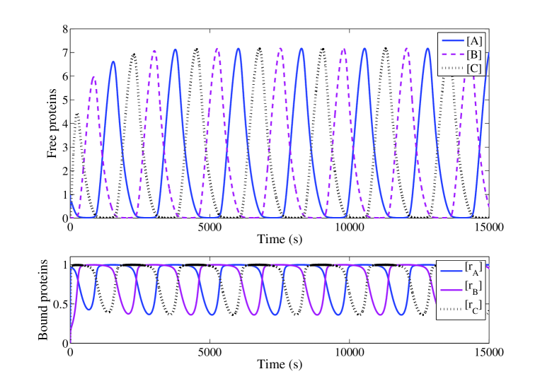
Figure 2: (color online) The numbers of free proteins (top) and bound proteins (bottom) of type $A$, $B$ and $C$, vs. time, for the repressilator with bound repressor degradation, obtained from numerical integration of the rate-equations. The parameters used are: $g=0.05$, $d=d_{r}=0.003$, $\alpha_{0}=0.5$ and $\alpha_{1}=0.01$ (s^-1). A regular pattern of oscillations is observed, with a phase delay of $120^{0}$ between successive proteins. The period of the oscillations is $\simeq 2260$ (s), and the maximal copy number is $\simeq 7$.

These equations exhibit oscillations for a broad range of parameters, and specifically for a broad range of values of $d_{r}$. These oscillations, shown in Fig. 2, are clearly non-sinusoidal. Indeed, the order of appearance of the dominant protein species is $A\to C\to B\to A$, as expected. The oscillations are symmetrical in the sense that the oscillation patterns for the three proteins are identical and each protein is dominant during about $1/3$ of the cycle. When different parameters are chosen for the three proteins, the amplitudes of their oscillations become different. Also, a protein that exhibits a larger amplitude maintains its dominance for a larger fraction of the oscillation period.

The parameter range in which oscillations are present shrinks to zero when $d_{r}\rightarrow 0$. We have analyzed the dependence of the oscillation period and amplitude on the parameters. It was found that the oscillation period, $T$, is dominated by the degradation rate of the proteins, namely $T\sim 1/d$. Since the lowest value of $[X_{i}]$ during the oscillation is typically nearly zero, the amplitude is given by $[X_{\rm max}]/2$, where $[X_{\rm max}]\sim g/d$ is the largest value of $[X_{i}]$.

As before, in the limit of fast binding and unbinding, one can obtain, from Eqs. (5), modified Michaelis-Menten equations of the form:

$$\dot{[X_{i}]}=\frac{g}{1+k[X_{i-1}]}-d[X_{i}]-{{d_{r}k}\over{1+k[X_{i}]}}[X_{i}].$$ (6)

These equations also exhibit oscillations, unlike the ordinary Michaelis-Menten Equations. The oscillations are very similar to those obtained from Eqs. (5). The effect of BRD on the oscillations can be understood from Eq. (6). This equation shows that BRD introduces a nonlinear degradation term to $[X_{i}]$. In this term, the degradation rate decreases as $[X_{i}]$ increases. This helps to destabilize the steady state solution. Small deviations from the steady state are enhanced because a protein that appears in small numbers has a higher degradation rate than a protein that appears in large numbers.

III.2 Repressilator with Cooperative Binding

In transcriptional regulation with cooperative binding, two or more copies of the transcription factor need to bind simultaneously to the promoter in order to perform the regulation. The number of simultaneously bound transcription factors needed to perform the regulation is given by $n$. The effect of cooperative binding was studied extensively before in the context of the genetic toggle switch, which consists of two genes which negatively regulate each other’s synthesis Cherry2000 ; Warren2004 ; Warren2005 ; Walczak2005 ; Lipshtat2006 ; Loinger2007 . It was found to have important effects on the function and stability of the genetic switch.

Here we focus on the repressilator circuit in the case of $n=2$. In particular, we consider the case in which pairs of identical proteins bind to each other and form dimers, namely, $X_{i}+X_{i}\rightarrow D_{i}$. When such dimer binds to a suitable promoter site, it negatively regulates the expression of the corresponding gene. In the analysis below we also account for the mRNA level, considering the transcription and translation as two separate processes. The rate-equations describing the repressilator system are

$$\left\{\begin{array}[]{l}\dot{[m_{i}]}=g_{m}\cdot(1-[r_{i-1}])-d_{m}[m_{i}]\\ \dot{[X_{i}]}=g_{p}[m_{i}]-d[X_{i}]-2\gamma[X_{i}]^{2}\\ \dot{[D_{i}]}=\gamma[X_{i}]^{2}-d_{D}[D_{i}]-\alpha_{0}[D_{i}](1-[r_{i}])+\alpha_{1}[r_{i}]\\ \dot{[r_{i}]}=\alpha_{0}[D_{i}](1-[r_{i}])-\alpha_{1}[r_{i}],\end{array}\right.$$ (7)

where $\gamma$ is the dimerization rate constant and $d_{D}$ is the degradation rate of the dimers. These equations exhibit oscillations within some range of parameters. We find that within the deterministic framework, including the mRNA level is sufficient in order to obtain oscillations. However, even if the mRNA level is ignored, oscillations take place if bound-repressor degradation is taken into account (Table II).

IV Stochastic Analysis

IV.1 Repressilator without Cooperative Binding

To account for stochastic effects we analyze the repressilator system using the master equation Paulsson2000 ; Kepler2001 ; Paulsson2002 and Monte Carlo (MC) simulations Gillespie1977 ; Mcadams1997 ; Mcadams1999 . The role of fluctuations is enhanced due to the discrete nature of the transcription factors and their binding sites, which may appear in low copy numbers. We also gain insight into the role of bound repressor degradation in the emergence of oscillations.

In the stochastic description of the system, we denote the number of free $X_{i}$ proteins by $N_{i}$, and the number of bound $X_{i}$ proteins by $r_{i}$. Using the master equation, we consider the time evolution of the probability distribution function $P(N_{A},N_{B},N_{C},r_{A},r_{B},r_{C})$, or in a more convenient notation $P(N_{1},N_{2},N_{3},r_{1},r_{2},r_{3})$. This is the probability for a cell to include $N_{i}$ copies of free protein $X_{i}$ and $r_{i}$ copies of the bound $X_{i}$ repressor, where $N_{i}=0,1,2,\dots$, and $r_{i}=0,1$ (assuming a single binding site). The master equation for the repressilator without cooperative binding takes the form

$$\dot{P}(N_{1},N_{2},N_{3},r_{1},r_{2},r_{3})=$$ (8)

$$\sum_{i=1,2,3}\{g\cdot(1-r_{i-1})[P(\dots,N_{i}-1,\dots,r_{1},r_{2},r_{3})-P(N_{1},N_{2},N_{3},r_{1},r_{2},r_{3})]$$

$$+d(N_{i}+1)[P(\dots,N_{i}+1,\dots,r_{1},r_{2},r_{3})-N_{i}P(N_{1},N_{2},N_{3},r_{1},r_{2},r_{3})]$$

$$+\alpha_{0}(N_{i}+1)r_{i}[P(\dots,N_{i}+1,\dots,r_{i}-1,\dots)-N_{i}(1-r_{i})P(N_{1},N_{2},N_{3},r_{1},r_{2},r_{3})]$$

$$+\alpha_{1}(1-r_{i})[P(\dots,N_{i}-1,\dots,r_{i}+1,\dots)-r_{i}P(N_{1},N_{2},N_{3},r_{1},r_{2},r_{3})]$$

$$+d_{r}(r_{i}+1)[P(N_{1},N_{2},N_{3},\dots,r_{i}+1,\dots)-r_{i}P(N_{1},N_{2},N_{3},r_{1},r_{2},r_{3})]\}.$$

The master equation has a single steady state solution, $\dot{P}(\vec{N})=0$, for all $\vec{N}=(N_{1},N_{2},N_{3},r_{1},r_{2},r_{3})$. This solution can be obtained by direct numerical integration of the master equation and it is always stable VanKampen1992 . The steady state solution of this master equation is not an equilibrium state, and therefore detailed balance is not satisfied. As a result, there is a net flow of probability between adjacent $\vec{N}$ states. The net flux of probability between states $\vec{N}$ and $\vec{N}^{\prime}$ is given by

$$\phi(\vec{N}\to\vec{N}^{\prime})=W(\vec{N}\to\vec{N}^{\prime})P(\vec{N})-W(\vec{N}^{\prime}\to\vec{N})P(\vec{N}^{\prime}),$$ (9)

where $W(\vec{N}\to\vec{N}^{\prime})$ is the transition rate from $\vec{N}$ to $\vec{N}^{\prime}$. Due to probability conservation, the flow of probability is organized in closed cycles.

To illustrate things, we consider the marginal probability distribution

$$P(N_{1},N_{2},N_{3})=\sum_{r_{1}=0}^{1}\sum_{r_{2}=0}^{1}\sum_{r_{3}=0}^{1}P(N_{1},N_{2},N_{3},r_{1},r_{2},r_{3}).$$ (10)

Oscillatory behavior of the repressilator is characterized by a regular cyclic pattern in the flow diagram $\phi(\vec{N}\to\vec{N}^{\prime})$, as observed in the marginal probability distribution. In this diagram, the flow is from the $A$ dominated region to the $C$ dominated region, then to the $B$ dominated region and back to the $A$ dominated region. Here we present results for a typical choice of parameters for bacteria such as E. coli. The values of these parameters are sensitive to the external conditions, such as the temperature and the nutritional supply. For a detailed list of parameters see Table 2.1 in Ref. Alon2006 and Table 2 in Ref. Arkin1998 . More specifically, the parameter values used here are $g=0.05$, $d=0.003$, $\alpha_{0}=0.5$ and $\alpha_{1}=0.01$ (s^-1). The protein synthesis rate $g$ represents typical synthesis times of proteins, which are of the order of 10 to 20 seconds. The degradation rate is consistent with typical half-life times of proteins and mRNAs vary in the range of several minutes Alon2006 ; Arkin1998 . The binding rate represents a time scale of diffusion across the cell and specific binding of a transcription factor to a DNA site, of the order of one second Elowitz2000 ; Alon2006 . The un-binding rate represents residence time on the DNA site of several minutes Elowitz2000 . It should be noted that the qualitative results are not sensitive to the specific choice of the parameters.

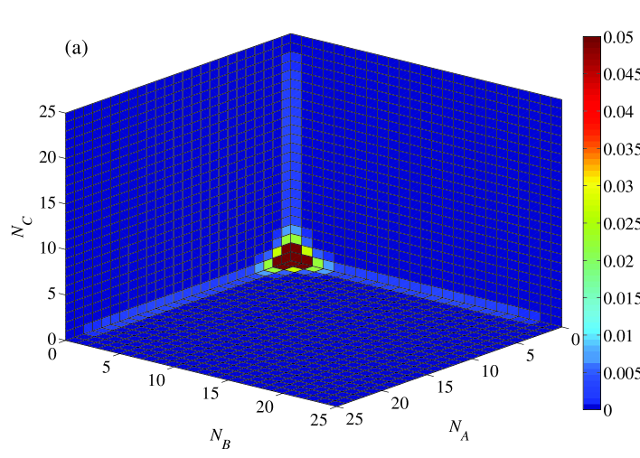
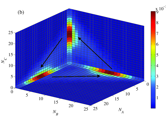
Figure 3: (color online) Slices of the probability distribution $P(N_{A},N_{B},N_{C})$ in the three planes $N_{A}=0$, $N_{B}=0$ and $N_{C}=0$ for the repressilator (the probability is represented by the color): (a) without degradation of the bound repressors, where most of the probability is concentrated near the origin, and there are no oscillations; (b) with degradation of the bound repressors, where $d_{r}=d=0.003$ (s^-1). In this case the system exhibit oscillatory behavior. Three peaks are observed, each of them dominated by one of the proteins. The probability flows between the peaks in the directions marked by the arrows.

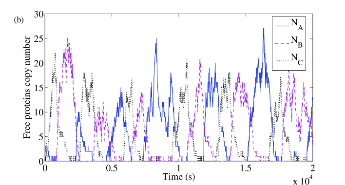
Figure 4: (color online) The number of free proteins of types $A$, $B$ and $C$, vs. time, for the repressilator, obtained from MC simulations: (a) without degradation of the bound repressors. In this case all the proteins are suppressed most of the time, with some irregular bursts; (b) with degradation of the bound repressors, where oscillations are observed. The oscillations are irregular both in their period and amplitude. The average period is $\simeq 3750$ (s), which is significantly longer than obtained from the rate-equations with the same parameters. The maximal number of proteins is also higher than in the rate-equation results.

In case that there is no degradation of bound repressors, namely $d_{r}=0$, there are no oscillations. The marginal probability distribution $P(N_{A},N_{B},N_{C})$ is highly concentrated near the origin [Fig. 3(a)]. In addition, there is a small probability that one of the proteins will have a high copy number while the other two genes are not expressed. We refer to this as a ’dead-lock’ situation. The production of all the proteins is suppressed by the simultaneous binding of bound repressors, and therefore oscillations cannot exist. The probability flux is small and also concentrated near the origin. MC simulations [Fig. 4(a)] show that indeed, most of the time, all the proteins appear in very low copy numbers (namely, two proteins or less). Occasionally, there is a burst in the population of one of the proteins, but no regular oscillations are observed.

In order to obtain oscillations we introduce degradation of the bound repressors. For simplicity, we assume that bound repressors degrade at the same rate as free repressors, namely $d_{r}=d=0.003$, leaving the other parameters as above. This prevents the ’dead-lock’ situation because degradation removes the bound repressors from the system. This is in contrast to un-binding, where the resulting free repressor may quickly bind again. In this case oscillations are observed. A similar effect was observed before in stochastic simulations of the toggle switch Lipshtat2006 ; Loinger2007 . It was found that BRD induces bistability by removing the dead-lock situation.

Under conditions in which oscillations take place, the probability distribution, $P(N_{A},N_{B},N_{C})$, exhibits three different peaks [Fig. 3(b)]. Each peak represents the stage of the oscillation in which the corresponding protein is dominant. The peaks are connected through regions with smaller, but non-vanishing probability. Through these regions probability flows between the three peaks (see arrows). MC simulations now show oscillatory behavior [Fig. 4(b)]. In these oscillations $C$ domination is followed by $B$ domination, then $A$ and returning to $C$. However, the oscillations are not regular. Both the period and the amplitude vary from one cycle to the next.

Since in MC simulations the oscillations are not regular, they are sometimes difficult to characterize. In order to identify the oscillations we use the fact that oscillatory systems exhibit a characteristic period, which can be evaluated using auto-correlation analysis. The auto-correlation function is defined by

$$F(\tau)=\left<N_{i}(t+\tau)N_{i}(t)\right>-\left<N_{i}(t)\right>^{2},$$ (11)

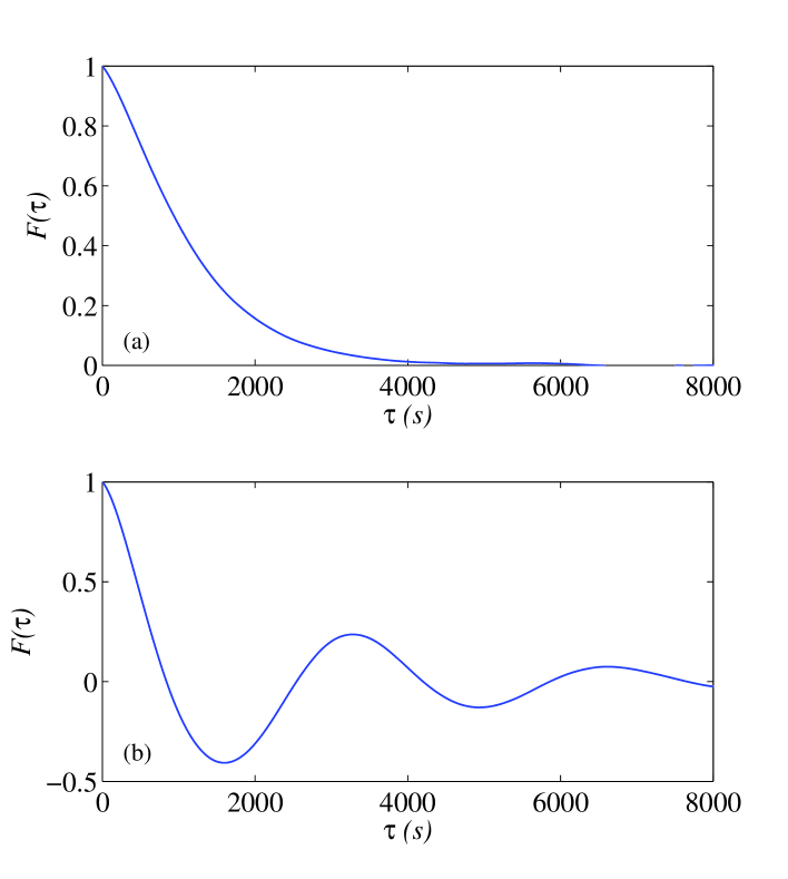
Figure 5: The Autocorrelation function $F(\tau)$ (normalized to unity), computed for the output of MC simulations: (a) in case there is no degradation of bound repressor ($d_{r}=0$). In this case the system does not exhibit oscillations. This is indicated by the autocorrelation function decaying monotonically to zero; (b) with degradation of bound repressor, $d_{r}=d=0.003$. In this case the system exhibits (irregular) oscillations. This is indicated by the autocorrelation function which exhibits several oscillations before it decays.

where $\left<\cdot\right>$ denotes averaging with respect to $t$. When the system does not exhibit oscillations, $F(\tau)$ decays monotonically to zero [Fig. 5(a)]. In case of oscillations, $F(\tau)$ oscillates before it decays [Fig. 5(b)]. The location of the first maximum of $F(\tau)$ provides the average period of the oscillations. The phase coherence time is determined by the number of the oscillations of $F(\tau)$ before it decays.

IV.2 Repressilator with Cooperative Binding

In the deterministic analysis of this version of the circuit, discussed in Sec. III B above, it was found that in order to obtain oscillations one needs to either include the mRNA level or to assume bound-repressor degradation (Table II). MC simulations of the same circuit indicate that in the stochastic case the situation is different. In this case the degradation of the bound repressors is a necessary condition for oscillations. The inclusion of the mRNA level does not affect the appearance of oscillations in this case.

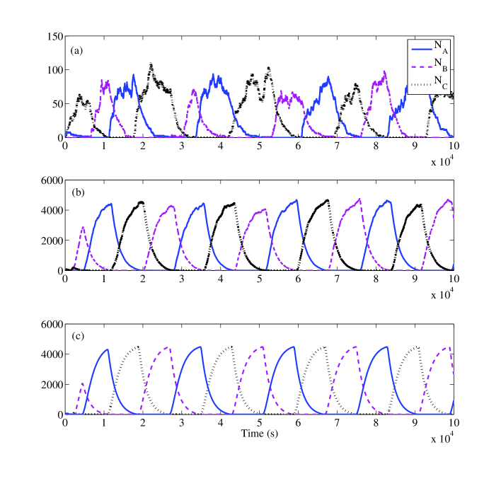
Figure 6: The number of free dimers, which consist of two proteins of types $A$, $B$ or $C$, for the repressilator with cooperative binding. (a) MC simulation results for a single plasmid; (b) MC simulation results for 50 plasmids; (c) Rate-equation results for 50 plasmids. Note that as the number of plasmids increases the rate-equation and MC results become identical.

In Fig. 6(a) we present the oscillations obtained from MC simulations of the repressilator with cooperative binding. The mRNA level is included, in order to obtain a more realistic description of the system. The MC simulations are based on the master equation for the probability $P(N_{i},r_{i},m_{i},D_{i})$, $i=1,2,3$, for the cell to contain $N_{i}$ free proteins and $r_{i}$ bound proteins of type $X_{i}$, as well as $m_{i}$ copies of mRNA and $D_{i}$ copies of the corresponding dimer. This master equation is not written explicitly here because it is cumbersome and adds little insight. It can be reproduced by starting from Eq. (8) and adding the terms that correspond to the synthesis and degradation of mRNAs as well as to dimer formation and degradation. Due to the higher dimensionality of this equation, direct integration becomes infeasible and MC simulations are used.

V The effect of the number of binding sites

We have examined the differences between the results obtained from deterministic and stochastic analysis of the repressilator circuit. We identified a case in which oscillations are obtained only in the rate-equations and are not obtained in MC simulations. This is the case of the repressilator with cooperative binding and without BRD, where the mRNA level is taken into account explicitly (Table II). Even when oscillations are obtained in both methods, there are differences between them. The oscillations obtained in the rate-equations are regular, and those obtained from the MC simulations are noisy and irregular. Moreover, the period and amplitude differ significantly between the rate-equations and the MC simulations. Below we discuss and try to resolve these differences.

The rate-equations deal with continuous quantities. These quantities are the averages, over an ensemble of cells, of the actual copy numbers of the proteins, which are discrete. The rate-equations involve some kind of ’mean field approximation’. In general, this approximation is justified when the copy numbers are large and the fluctuations can be ignored. However, in our case, an essential part of the system, namely the bound repressors, always appear in small numbers, 0 or 1. Therefore, the assumption of large copy numbers fails, and the validity of the rate-equations is questionable.

The rate-equations can describe the system in a correct manner only in the limit of high copy numbers of bound repressors. Interestingly, this situation can, in fact, be realized in cells by placing the relevant genes on plasmids, as done in Ref. Elowitz2000 . Plasmids are small circular segments of DNA that may exist in the cell and can be inserted synthetically. The number of plasmids in the cell, $n_{p}$, can be controlled. The number of binding sites that regulate a particular gene, which appears on the plasmids is equal to $n_{p}$ if this gene does not appear on the chromosome. If it is also present on the chromosome, the number of such binding sites is $n_{p}+1$. Here we assume, for simplicity, that the number of the binding sites is $n_{p}$. Taking this into account, appropriate changes must be made in the equations describing the system. The number of bound repressors, $r_{i}$, can now take the values $0\leq[r_{i}]\leq n_{p}$ in the rate-equations and the values $r_{i}=0,1,\dots n_{p}$, in the master equation. In both cases, the expression $1-r_{i}$ should be replaced by $n_{p}-r_{i}$. For example, Eq. (3) becomes

$$\left\{\begin{array}[]{l}\dot{[X_{i}]}=g\cdot(n_{p}-[r_{i-1}])-d[X_{i}]-\alpha_{0}[X_{i}]\left(n_{p}-[r_{i}]\right)+\alpha_{1}[r_{i}]\\ \dot{[r_{i}]}=\alpha_{0}[x_{i}]\left(n_{p}-[r_{i}]\right)-\alpha_{1}[r_{i}].\end{array}\right.$$ (12)

In the limit of a large number of plasmids, an agreement is obtained between the rate-equation and the MC results. This agreement is both qualitative and quantitative. Qualitatively, for a high plasmid copy number, the system exhibits oscillations in the rate-equations if and only if it exhibits oscillations in the MC simulations. Consider, for example, the repressilator with dimers and without BRD, where the mRNA level is taken into account. For $n_{p}=1$ the system exhibits oscillations in the rate-equations but not in the MC simulations. As $n_{p}$ increases, the oscillations in the rate-equations disappear and become consistent with the MC results.

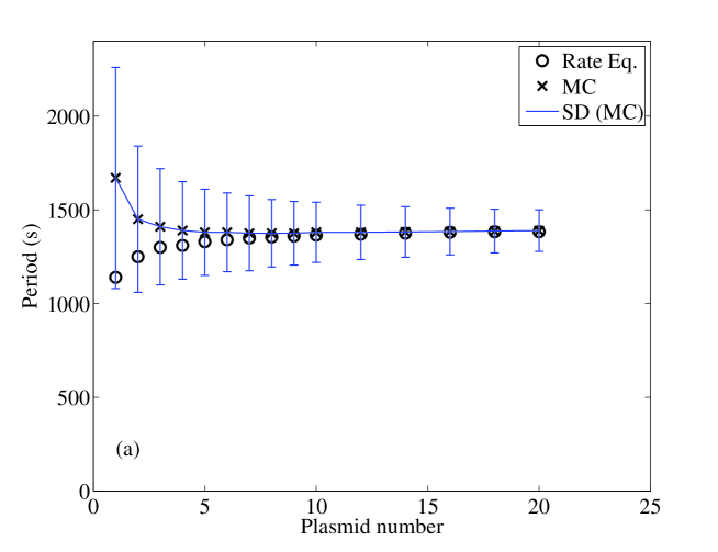
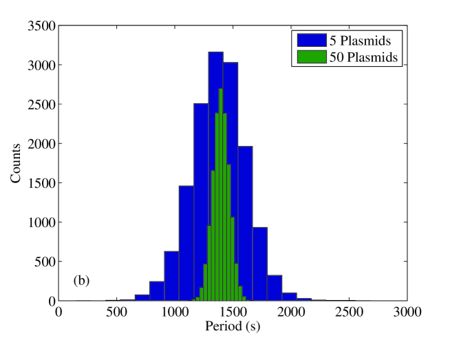
Figure 7: (a) Comparison between the period of the oscillations obtained from MC simulations and from rate-equations for the same parameters, vs. the plasmid copy number. For a small number of plasmids the periods differ, but for a large number of plasmids, they approach the same value. The error bars represent one standard deviation (SD); (b) The distribution of the periods of oscillations obtained from MC simulations for 5 and 50 plasmids. The distribution is approximately a Gaussian with almost the same average. The Gaussian is much narrower for the high plasmid copy number. This indicates that the oscillations become more regular when a large number of plasmids is present in the cell.

In case that the number of plasmids is small, the average period of the oscillations in the MC simulations may differ from the period obtained in the rate-equations. However, for a large number of plasmids, the oscillations obtained in the MC simulations become much more regular, and more similar in shape to those obtained from the rate-equations, with the same number of plasmids [Fig. 6]. In this case the two periods converge towards each other [Fig. 7(a)]. The distribution of the periods in the MC simulations becomes narrower as the number of plasmids increases [Fig. 7(b)], and the oscillations become more regular.

VI Summary

We have analyzed the genetic repressilator circuit using deterministic and stochastic methods. In particular, we examined the effects of cooperative binding, the degradation of bound repressors and the inclusion of the mRNA level in the model. The qualitative results are summarized in Table II. Due to the small numbers of proteins and binding sites, stochastic effects are significant and the deterministic analysis may fail. It fails qualitatively in the biologically relevant case in which there is cooperative binding, the mRNA level is taken into account and no BRD is assumed. In this case the rate-equations predict oscillations which do not appear in the stochastic analysis. In addition, even when the deterministic and stochastic methods agree about the existence of oscillations, there are quantitative differences in the period, amplitude and regularity of the oscillations as well as in the range of parameters in which they appear.

Since the repressilator was encoded on plasmids we have studied the effect of increasing the number of plasmids in a cell on the behavior of the system. We found that as the number of plasmids increases, the role of fluctuations is suppressed and the rate-equations become valid. The results show that varying the plasmid copy number may lead to qualitative changes in the dynamics of genetic circuits. This prediction can be tested experimentally in the context of synthetic biology and should be taken into account in the design of artifical genetic circuits.

Our results indicate that deterministic analysis is valid only in the limit in which all the components, namely mRNAs and both free and bound proteins, appear in large copy numbers. This condition is not satisfied in genetic circuits encoded on the chromosome. Thus, for these circuits deterministic methods may fail. In particular, in cases in which the system exhibits multiple steady states Lipshtat2006 ; Loinger2007 or oscillations, deterministic and stochastic methods may yield qualitatively different results. In these cases, the system may be sensitive to subtle features such as cooperative binding, BRD and the inclusion of the mRNA level in the model. Thus, in the modeling of these systems, such features should be taken into account. In addition, our results provide strong evidence for the existence of degradation of bound proteins. This result has significant biological implications beyond the specific circuit studied here.

We thank N.Q. Balaban for many helpful discussions.

Table 1: The existence of oscillations vs. the Hill-coefficient $n$ in the Michaelis-Menten equations, with and without the inclusion of the mRNA level. The mRNA level is included in Eq. (1) and is not included in Eq. (2). In both cases, we did not include bound-repressor degradation. The cases in which the system exhibits oscillations are marked by $\surd$ and those in which it does not are marked by $\times$.

Hill-coefficient	with mRNA	without mRNA
1	$\times$	$\times$
2	$\surd$	$\times$
3	$\surd$	$\surd$

Table 2: Oscillations in different variants of the repressilator. The cases in which the system exhibits oscillations are marked by $\surd$ and those in which it does not are marked by $\times$. The following features are taken into account: cooperative vs. non-cooperative regulation, the inclusion vs. non-inclusion of the mRNA level in the model and degradation vs. non-degradation of bound repressors. Here, cooperative circuits refer to repression by protein dimers. The deterministic analysis is done using the complete set of rate-equations and the stochastic analysis is done using MC simulations. Note that in cases in which both the deterministic and stochastic approaches exhibit oscillations, the parameter range in which they appear may differ. In the limit of high plasmid copy number, the results obtained from the deterministic and stochastic method coincide. The results reported in this Table are based on linear stability analysis and on a large number of simulations covering the biologically relevant range of the parameter space with a fine grid.

Circuit variant			Low plasmid copy number		High plasmid copy number
	mRNA	BRD	Deterministic	Stochastic	Deterministic and Stochastic
	No	No	$\times$	$\times$	$\times$
	Yes	No	$\times$	$\times$	$\times$
Non-Cooperative	No	Yes	$\surd$	$\surd$	$\surd$
	Yes	Yes	$\surd$	$\surd$	$\surd$
	No	No	$\times$	$\times$	$\times$
	Yes	No	$\surd$	$\times$	$\times$
Cooperative	No	Yes	$\surd$	$\surd$	$\surd$
	Yes	Yes	$\surd$	$\surd$	$\surd$

Figure 1: Schematic plot of the repressilator circuit. It consists of three genes which negatively regulate each other by transcriptional regulation in a cyclic order.

References

- (1) U. Alon, An introduction to systems biology: design principles of biological circuits (Chapman & Hall/CRC, London, 2006).
- (2) B.Ø. Palsson, Systems biology: properties of reconstructed networks (Cambridge University Press, Cambridge, 2006).
- (3) R. Milo, S. Shen-Orr, S. Itzkovitz, N. Kashtan, D. Chklovskii and U. Alon, Science 298, 824 (2002).
- (4) R. Milo, S. Itzkovitz, N. Kashtan, R. Levitt, S. Shen-Orr, I. Ayzenshtat, M. Sheffer and U. Alon, Science 303, 1538 (2004).
- (5) E. Yeger-Lotem, S. Sattath, N. Kashtan, S. Itzkovitz, R. Milo, R.Y. Pinter, U. Alon and H. Margalit, Proc. Natl. Acad. Sci. US 101, 5934 (2004).
- (6) S. Mangan and U. Alon, Proc. Natl. Acad. Sci. US 100, 11980 (2003).
- (7) M. Ptashne, A Genetic Switch: Phage and Higher Organisms (Cell Press and Blackwell Scientific Publications, Cambridge, MA, 1992).
- (8) P. Francois and V. Hakim, Phys. Rev. E 72, 031908 (2005).
- (9) Y. Artzy-Randrup,S.J. Fleishman, N. Ben-Tal and L. Stone, Science 305, 1107 (2004).
- (10) A. Mazurie, S. Bottani and M. Vergassola, Genome Biol. 6, R35 (2005).
- (11) O. Meshi, T. Shlomi and E. Ruppin, BMC Systems Biol. 1, 1 (2007).
- (12) M.B. Elowitz and S. Leibler, Nature 403, 335 (2000).
- (13) T.S. Gardner, C.R. Cantor and J.J. Collins, Nature 403, 339 (2000).
- (14) M.B. Elowitz, A.J. Levine, E.D. Siggia and P.S. Swain, Science 297, 1183 (2002).
- (15) E.M. Ozbudak, M. Thattai, I. Kurtser, A.D. Grossman and A. van Oudenaarden, Nature Genetics 31, 69 (2002).
- (16) H.H. McAdams and A. Arkin, Proc. Natl. Acad. Sci. US 94, 814 (1997).
- (17) H.H. McAdams and A. Arkin, Trends Genet. 15, 65 (1999).
- (18) J. Paulsson, Nature 427, 415 (2004).
- (19) A. Becskei and L. Serrano, Nature 405, 590 (2000).
- (20) M. Kaern, T.C. Elston, W.J. Blake and J.J. Collins, Nature Reviews Genetics 6, 451 (2005).
- (21) Rosenfeld, N., Elowitz, M.B., Alon, U., J. Mol. Biol. 323, 785 (2002).
- (22) T.B. Kepler and T.C. Elston, Biophys. J. 81, 3116 (2001).
- (23) M. Sasai and P. Wolynes, Proc. Natl. Acad. Sci. US 100, 2374 (2003).
- (24) W.T. Mocek, R. Rudnicki, and E.O. Voit, Math. Biosci. 198, 190 (2005).
- (25) L. Chen and K. Aihara, IEEE Trans. Circuits Syst. I 49, 602 (2002).
- (26) J. Lewis, Curr. Biol. 13, 1398 (2003).
- (27) N.A. Monk, Curr. Biol. 13, 1409 (2003).
- (28) D. Bratsun, D. Volfson, L. S. Tsimring, and J. Hasty, Proc. Natl. Acad. Sci. U.S.A. 102, 14593 (2005)
- (29) J.S. Griffith, J. Theor. Biol.20, 202 (1968).
- (30) J.E.M. Hornos, D. Schultz, G.C.P. Innocentini, J. Wang, A.M. Walczak, J.N. Onuchic and P.G. Wolynes, Phys. Rev. E 72, 051907 (2005).
- (31) K.Y. Kim, D. Lepzelter, and J. Wang, J. Chem. Phys. 126, 034702 (2007).
- (32) A. Lipshtat, A. Loinger, N. Q. Balaban and O. Biham, Phys. Rev. Lett. 96, 188101 (2006).
- (33) A. Loinger, A. Lipshtat, N. Q. Balaban and O. Biham, Phys. Rev. E 75, 021904 (2007).
- (34) J.L. Cherry and F.R. Adler, J. Theor. Biol. 203, 117 (2000).
- (35) P.B. Warren and P.R. ten Wolde, Phys. Rev. Lett. 92, 128101 (2004).
- (36) P.B. Warren and P.R. ten Wolde, J. Phys. Chem. B 109, 6812 (2005).
- (37) A. M. Walczak, M. Sasai, and P. Wolynes, Biophys. J. 88, 828 (2005).
- (38) J. Paulsson and M. Ehrenberg, Phys. Rev. Lett. 84, 5447 (2000).
- (39) J. Paulsson, Genetics 161, 1373 (2002).
- (40) D.T. Gillespie, J. Phys. Chem. 81, 2340 (1977).
- (41) N.G. Van Kampen, Stochastic processes in physics and chemistry (Elsevier, North-Holland, 1992).
- (42) A. Arkin, J. Ross and H.H. McAdams, Genetics 149, 1633 (1998).