Traffic of molecular motors: from theory to experiments

Intracellular transport along microtubules or actin filaments, powered by molecular motors such as kinesins, dyneins or myosins, has been recently modeled using one-dimensional driven lattice gases. We discuss some generalizations of these models, that include extended particles and defects. We investigate the feasibility of single molecule experiments aiming to measure the average motor density and to locate the position of traffic jams by mean of a tracer particle. Finally, we comment on preliminary single molecule experiments performed in living cells.

I Introduction

Living cell is a highly organised structure that constantly needs to move its constituent parts from one place to another. It is therefore provided with a complex and accurate distribution system: the cytoskeleton, the network of biopolymers (actin, microtubules and intermediate filaments) that gives the cell its structural and mechanical features, functions as road system for the transport of organelles and vesicles; the motion of these objects is entrusted to motor proteins moving along these filaments. These motors are enzymes that convert the energy obtained by hydrolysis of an ATP (adenosin-triphosphate) molecule into a work (displacement of their cargo). Myosin V (on actin filament) and kinesin or dynein (on microtubules) are well known examples of these so called processive motors b:alberts-etal:02 ; b:howard:01 .

It has been observed that these motors can act cooperatively or interact with each other giving rise to collective phenomena. In particular, in some phase of the cell cycle, the motors can be expressed in high concentrations: it seems therefore natural to investigate analogies and differences with the traffic observed in a city. Experimental techniques as single molecule and fluorescence imaging have just started giving some hints on the complex behaviour of this system, but are still far from giving quantitative description of traffic situations. While waiting for experimental data some theoretical models have been developed to physically describe intracellular transport.

II Driven lattice gases: models for intracellular transport

A simple model to capture the behavior of many motors on a filaments needs to include three fundamental features: (i) the motors move in a step-like fashion on a one dimensional tracks and bind specifically to the monomer constituting the cytoskeletal filaments; (ii) cytoskeleton filaments present a specific polarization: the chemical properties of the track guarantee that the motion is always directed towards one of the two ends of the filament; (iii) the particles move according to a stochastic rule, i.e. they move upon a chemical reaction, the hydrolysis of ATP, which occurs randomly with a typical rate.

The Total Asymmetric Simple Exclusion Process (TASEP) is a stochastic process first introduced to describe the motion of ribosomes on mRNA substrate macdonald-gibbs-pipkin:68 and encodes all these features. It rapidly became a paradigm of non-equilibrium statistical mechanics and one of the few example of exactly solvable systems derrida-domany-mukamel:92 ; schuetz-domany:93 . In this model each particle occupies a site on a one dimensional lattice and advances stochastically and in one direction. The most obvious observable is the average density profile of particles along the lattice.

The system with open boundaries where particles enter the lattice with rate $\alpha$ at one end and leave with rate $\beta$ at the other, shows a non trivial phase diagram where three distinct non-equilibrium steady states appear: a low density phase controlled by the left boundary, a high density phase controlled by the right boundary and a maximal current phase, independent of the boundaries.

\psfrag{alpha}{$\alpha$}\psfrag{beta}{$\beta$}\psfrag{a}{$a$}\psfrag{i=1}[c]{$i=1$}\psfrag{i=N}[c]{$i=N$}\psfrag{tau=1}[l]{$\tau=1$}\psfrag{omega_A}[c]{$\omega_{A}$}\psfrag{omega_D}[c]{$\omega_{D}$}\psfrag{a}{(a)}\psfrag{b}{(b)}\includegraphics[width=433.62pt]{model.eps}

Figure 1: Schematic representation of the TASEP with Langmuir kinetics in the case of (a) monomers and (b) dimers. The allowed moves are: forward jump (with rate $\tau=1$), entrance at the left boundary (with rate $\alpha$), exit at the right boundary (with rate $\beta$), attachment (with rate $\omega_{A}$), and detachment (with rate $\omega_{D}$) in the bulk.

In a first attempt to construct a minimal model for molecular intracellular transport, one needs to add to the TASEP the fact that the tracks are embedded in the cytosol with a reservoir of motors in solution. This allows the motors to attach to or detach from the track. This led to the construction of the TASEP with Langmuir (i.e. attachment/detachment) kinetics or TASEP/LK model parmeggiani-franosch-frey:03 ; parmeggiani-franosch-frey:04 depicted in Fig. 1a. According to this model, in addition to the TASEP properties, particles enter (leave) the system with rate $\omega_{A}$ ($\omega_{D}$) also in the bulk. All over the lattice they obey exclusion: two particles cannot occupy the same site.

According to the rules described above, the rate equation in the average density at site $i=2\dots N$, $\left\langle n_{i}\right\rangle$ can be written as:

$$\partial_{t}\left\langle n_{i}\right\rangle=\left\langle n_{i-1}\left(1-n_{i}\right)\right\rangle-\left\langle n_{i}\left(1-n_{i+1}\right)\right\rangle+\left[\omega_{A}(1-\left\langle n_{i}\right\rangle)-\omega_{D}\left\langle n_{i}\right\rangle\right]\,.$$ (1)

The first two brackets describe the average current and the second one the on-off kinetics (source and sink terms). At the boundaries this equation reads:

$$\partial_{x}\left\langle n_{1}\right\rangle = \alpha\left(1-\left\langle n_{i}\right\rangle\right)-\left\langle n_{1}\left(1-n_{2}\right)\right\rangle\,,$$ (2)

$$\partial_{x}\left\langle n_{N}\right\rangle = \left\langle n_{N-1}\left(1-n_{N}\right)\right\rangle-\beta\left\langle n_{N}\right\rangle\,.$$ (3)

Equation (1) shows a non-closed hierarchy in the correlation functions (i.e. $\left\langle n_{i}\right\rangle$ depends on $\left\langle n_{i}n_{j}\right\rangle$ and so on): this suggests the use of the mean field approximation $\left\langle n_{i}n_{i+1}\right\rangle\approx\left\langle n_{i}\right\rangle\left\langle n_{i+1}\right\rangle$. In the stationary state, the leading term of the continuum limit ($N\to\infty$, $\left\langle n_{i}\right\rangle\to\rho(x)$) of Eq. (1) reads:

$$-\partial_{x}\left[\rho(1-\rho)\right]+\left[\Omega_{A}(1-\rho)-\Omega_{D}\rho\right]=0\,,$$ (4)

supplemented by two boundary conditions: $\rho(0)=\alpha$ and $\rho(1)=1-\beta$ parmeggiani-franosch-frey:03 . When the solution of Eq. (4) cannot be matched continuously with the left and right boundaries, the density profile displays a localized discontinuity (or shock) in the bulk (Figs. 2b-c). This translates into the emergence of mixed phases that were not present in the simple TASEP. For some sets of parameters the phase diagram can exhibit up to 7 kinds of coexistence (see Fig.2a).

A key point in the study of TASEP/LK is the introduction of a mesoscopic limit where local adsorption-desorption rates $\omega_{A,D}$ have been rescaled in the limit of large but finite systems $\omega_{A,D}=\Omega_{A,D}/N$, such that the macroscopic rates are comparable to the injection-extraction rates at the boundaries parmeggiani-franosch-frey:03 . Far from being only a simple mathematical trick that allows the competition of the directed motion with the on-off kinetics, this limit captures the fact that the motors explores a significant fraction of the track before detaching. This is precisely the limit of highly processive motors that biologically motivated our studies. Surprisingly only in the mesoscopic limit the density profiles show the shock.

\psfrag{r}[1][-90]{$\rho$}\psfrag{j}[1][-90]{$j$}\psfrag{x}{$x$}\psfrag{(a)}{(a)}\psfrag{(b)}{(b)}\psfrag{(c)}{(c)}\psfrag{beta}{$\beta$}\psfrag{alpha}{$\alpha$}\psfrag{a*}[l]{$\alpha^{*}=1/2$}\psfrag{b*}[c]{$\beta^{*}=1/2$}\psfrag{LD}[0.8]{LD}\psfrag{HD}[0.8]{HD}\psfrag{LD/HD}[0.8]{LD/HD}\psfrag{MC/HD}[0.8]{MC/HD}\psfrag{LD/MC}[0.8]{LD/MC}\psfrag{MC}[0.8]{MC}\psfrag{LD/MC/HD}[0.8]{LD/MC/HD}\psfrag{X0}{$x_{w}=0$}\psfrag{X1}{$x_{w}=1$}\psfrag{0}[bl]{0}\psfrag{1}[bl]{1}\psfrag{ 0}[bl]{0}\psfrag{ 1}[bl]{1}\psfrag{ 0.2}[bl]{0.2}\psfrag{xw}{$x_{w}$}\psfrag{ra}{$\rho_{\alpha}$}\psfrag{rb}{$\rho_{\beta}$}\psfrag{ja}{$j_{\alpha}$}\psfrag{jb}{$j_{\beta}$}\includegraphics[width=433.62pt]{taseplk.eps}

Figure 2: (a) Phase diagram of TASEP/LK for $\omega_{A}=\omega_{D}$. One recognizes seven phases: in addition to the TASEP low density (LD), high density (HD) and maximal current (MC) phases; there are four more coexistence phases, namely the LD/HD, LD/MC, MC/HD and LD/MC/HD phases. The shaded region highlights the LD/HD coexistence where a localized domain wall appears. (b) Typical density profile in the LD/HD phase and (c) the corresponding current profile. At the matching point $x_{w}$ between the left ($j_{\alpha}$) and right ($j_{\beta}$) currents a domain wall develops and connects the left ($\rho_{\alpha}$) and right ($\rho_{\beta}$) density profile.

III Extending the model: dimers and defects

III.1 Dimers

Many processive molecular motors (kinesins, dyneins and myosin V) are composed of two heads that bind specifically each to a subunit of the molecular track. A natural extension of the previous model towards a more realistic one consists in introducing non-pointlike particles in the system such as dimers (see Ref. pierobon-frey-franosch:06 and Fig. 1b). There are several challenging aspects in this problem: (i) the TASEP of particles of size $\ell$ (or $\ell$-TASEP) is known to have a non-trivial current-density relation $j(\rho$), different from the model with monomers chou-lakatos:04 ; macdonald-gibbs-pipkin:68 ; shaw-zia-lee:03 ; (ii) even the simple on-off kinetics of dimers exhibits non-trivial dynamics, for example the stationary state is reached from an empty system through a double step relaxation process mcghee-hippel:74 ; frey-vilfan:02 . The coupling of an equilibrium process with two intrinsic relaxation regimes (on-off kinetics) to a genuine driven process (the $\ell$-TASEP) suggests interesting dynamical phenomena likely to result in new phases and regimes.

In absence of exact solution, the main challenge has been to construct a refined mean field theory, based on probability theory, and to prove the consistency of the approximation for the two competing process (TASEP and the on-off kinetics). We have solved the mean field equation within the mesoscopic limit in the stationary state:

$$-\partial_{x}\left[\frac{\rho(1-2\rho)}{1-\rho}\right]+\left[\Omega_{A}\frac{(1-2\rho)^{2}}{(1-\rho)}-\Omega_{D}\rho\right]=0\,.$$ (5)

The complete equation is formally similar to the one for pointlike particles (Eq.4): the current term (first bit in square brackets) must be balanced by the on-off term (second part).

Exploiting the analytical properties of the solution of the mean field equation and the local continuity of the current, we constructed the global density profile. We have performed extensive stochastic simulations and the agreement with the mean field solution is excellent. As in the case of TASEP/LK of monomers a new phase coexistence region appears for some parameters. The main effect of extended nature of dimers on the phase behavior of the system is related to the breaking of the (particle-hole) symmetry of the model. This does have quantitative but not qualitative consequences on the density profile and on the phase diagram, which remains topologically unchanged. The origin of the robustness of the picture found for monomers can be traced back to the form of the stationary density profile which depends exclusively on the form of the current-density relation and of the isotherm of the on-off kinetics. In both the monomer and the dimer case the current-density relation is concave and presents a single maximum, while the isotherm is unique and constant: these two features are enough to determine the topology of the phase diagram. This robustness suggests that the TASEP dynamics washes out the interesting two-step relaxation dynamics that characterizes the on-off kinetics of dimers: the non-trivial outcome is that, in these systems, the diffusion (yet asymmetric) always dominates the large time-scale relaxation.

III.2 Defect

Another question that often arises in the study of these models concerns the role of some kind of randomness: the motion of the particles can be altered by structural defects of the track or by microtubule associated proteins (MAP). A good modeling requires to introduce some sort of disorder in the system: site-related or particle related, quenched or annealed. While disorder in TASEP has been treated with exact and approximated methods harris-stinchcombe:04 ; juhasz-santen-igloi:05 ; kolwankar-punnoose:00 ,the role of bottlenecks was never coupled to the TASEP/LK. As a preliminary study of the role of quenched disorder, it becomes particularly interesting to investigate the influence of an isolated defect (i.e. point-wise disorder) on the stationary properties of the TASEP/LK. In Ref.pierobon-etal:06 we extensively studied this model where the defect has been characterized by a reduced hopping rate $q<1$ (see Fig. 3).

As a consequence of the competition between the TASEP and LK dynamics, the effects of a single bottleneck in the TASEP/LK model are much more dramatic than in the simple TASEP kolomeisky:98 (or the TASEP for extended objects shaw-kolomeisky-lee:03 ), where a localized defect was shown to merely shift some transition lines in the phase-diagram, but do not affect its topology. Here, new and mixed phases induced by the bottleneck have been obtained.

As a key concept of our analysis, we have introduced the carrying capacity, which is defined as the maximal current that can flow through the bulk of the system. In contrast to the simple TASEP the spatial dependence of the current, caused by the Langmuir kinetics, makes the carrying capacity non-trivial: the defect depletes the current profile within a distance that we called screening length. This quantity increases with the strength of the defect and decreases with the attachment-detachment rates. The competition between the current imposed at the boundaries and the one limited by the defect determines the density profiles and the ensuing phase-diagram. When the boundary currents are dominant, the phase behavior of the defect-free system is recovered. Also, above some critical entrance and exit rates, the system transports the maximal current, independently of the boundaries. Between these two extreme situations, we have found several coexistence phases, where the density profile exhibits stable shocks and kinks. Indeed, above some specific parameter values the phase-diagram is characterized by bottleneck phases. Depending on the screening length imposed by the defect, which can cover the entire system or part of it, different phase-diagrams arise. The latter are characterized by four, six or even nine bottleneck phases, which have been quantitatively studied within the mean-field theory introduced in Sec.II: in fact for entrance and exit rates that exceed the critical value $q/(1+q)$ (for which the bottleneck becomes relevant) the system can be split in two sublattices that can be treated as independent TASEP/LK with effective exit/entrance rates at the junction (Fig. 3a).

Our results were checked against numerical simulations, which brings further arguments in favor of the validity of mean-field approaches for studying the TASEP/LK-like models (Figs.3b-c). The somewhat surprising quantitative validity of this approximate scheme can be traced back to the current-density relationship, which is correctly predicted by the mean-field theory.

Eventually, we think that this study showed clearly that the presence of disorder in the TASEP/LK model, even in its simplest form, generally gives rise to quite rich and intriguing features and should motivate further studies of more ‘realistic’ and biophysically relevant situations, as in the presence of clusters of competing defects or quenched site-wise randomness (where the motors are slowed down at several points in the system).

\psfrag{a}{(a)}\psfrag{b}{(b)}\psfrag{c}{(c)}\psfrag{i=1}{$1$}\psfrag{i=N}{$N$}\psfrag{i=k}{$k$}\psfrag{L}{${\cal L}$}\psfrag{tau=1}{$r=1$}\psfrag{q}{$q<1$}\psfrag{omega_A}{$\omega_{A}$}\psfrag{omega_D}{$\omega_{D}$}\psfrag{alpha}{$\alpha$}\psfrag{beta}{$\beta$}\psfrag{alphaeff}{$\alpha_{\textrm{eff}}$}\psfrag{betaeff}{$\beta_{\textrm{eff}}$}\psfrag{ralpha}[l]{$\rho_{1}=\alpha$}\psfrag{rbeta}[d]{$\rho_{N}\!=\!1\!-\!\beta$}\psfrag{ralpha1}[l]{$\rho(0)=\alpha$}\psfrag{rbeta1}[d]{$\rho(1)\!=\!1\!-\!\beta$}\psfrag{q1}[l]{$\rho_{k}$}\psfrag{q2}[l]{$\rho_{k+1}$}\psfrag{q1a}[c]{$\frac{1}{1-q}$}\psfrag{q2a}[c]{$\frac{q}{1-q}$}\psfrag{q}{$q$}\psfrag{x=k}{$i=k$}\psfrag{I}{L}\psfrag{II}{R}\psfrag{x}{$x$}\psfrag{j}{$j$}\psfrag{r}{$\rho$}\includegraphics[width=433.62pt]{defect.eps}

Figure 3: (a) Cartoon representing the TASEP/LK with a bottleneck: above a threshold density the system can be divided into two lattices where the results of TASEP/LK are valid. (b) Density and (c) current in a case where the bottleneck is relevant and competes with the boundaries leading to the formation of a double domain wall, theoretical results (dashed lines) are superimposed to numerical simulations (bold line).

IV Towards the experiments

IV.1 Tracer dynamics

All the models described so far would be rather useless without the possibility to measure quantitatively the density and to localize the shock. To this aim, simple bulk fluorescence imaging would be difficult to apply to quantitative experiments: single molecule analysis are far more promising. We proposed hence a method, based on single particle tracking, to measure the density of the system phd:pierobon . The idea is to use the simple TASEP (exact) results to reconstruct the density from the velocity or the diffusion constant of the tracer. It is known that the average velocity $v\equiv\frac{d\left\langle x(t)\right\rangle}{dt}$ is related to the density $\rho$ through the relation $\rho=1-v$. Exact results on a ring show that the same relation holds for the diffusion constant $D\equiv\frac{\left\langle x^{2}\right\rangle-\left\langle x\right\rangle^{2}}{t}=1-\rho$ derrida-evans-mukamel:93 .

Since the rates scales with the size of the system, according to the mesoscopic limit, we suppose that the influence of attachment detachment on this relation to be negligible and the density to be locally continuous. We simulated the system TASEP/LK and measured the position $x$ as a function of the time for several particles, in order to construct the probability density function $P(x,t,|0,0)$ to find a tracer particle at site $x$ after a time $t$ from its entrance in the system at site $0$. From this function we can measure the velocity and the diffusion constant. As shown in Fig. 4, the shock is localized within a $10\%$ precision through both the indicators. While the density is well reconstructed from the information on the velocity (Fig. 4a), the hypothesis $\rho=1-D$ works well only in the low density phase before the particle arrives at the shock. Once the particle has passed through the shock the hypothesis on the continuity of the density breaks down and the relation is not valid anymore while the loss of particles in the high density phase makes the system subdiffusive. Yet, the quantity $1-D$ can be used to localized the shock (Fig. 4b).

Numerical simulations show that, on system of realistic size (i.e. $1\mu m$, roughly 100 sites), analysing the trajectories of a hundred particles is enough to reconstruct the density profile and localize the shock (after a time moving average resulting on a smoothing of the data). This suggests that single molecule experiments observing local features could give information on the global scale.

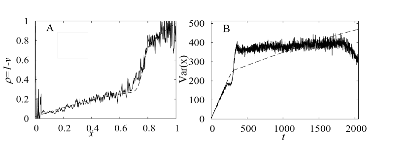
Figure 4: (a) Density profile of TASEP/LK derived from the analysis of 100 tracer particles: wiggly line match rather well the theoretical prediction (dashed line). (b) Superposition of the first two moments of $P(x,t)$, $\left\langle x\right\rangle(t)$ (dashed) and $Var[x(t)]$ (wiggly) in time: according to the simple TASEP results the two quantities should be the same; this is true only until the particles have reached the shock, afterwards the variance deviates.

IV.2 Single molecule in the cell

So far much information concerning processive molecular motors was provided by single molecule experiments. Typically a latex bead is attached to the motor to make it visible and to manipulate it: this allowed us to measure not only velocity and processivity of the motors, but even the forces they exert, the steps and (in some lucky cases) substeps veigel-etal:02 ; uemura-etal:04 ; dunn-spudich:07 ; cappello-etal:07 . In-vitro observations can be quite controversial: some experiments did not show any difference upon increasing the concentrations of motors, as if traffic effects were not relevant seitz-surrey:06 . However the situation in the overcrowded environment of the cell is hardly reproducible in vitro and could reserve more surprises.

Since single molecule experiments have often been criticized because of their distance from the real systems, many groups are cautiously moving the single molecule experiments directly into the cell dahan-etal:03 ; selvin-etal:05 ; xie-yu-yang:06 ; watanabe-higuchi:07 . In this situation the main problem is to have a good signal-noise ration which is hardly achievable with the usual fluorescent probes. Recently a method to mark and observe single molecule in vivo by using quantum dots (QDs) has been proposed courty-etal:06 ; xie-yu-yang:06 . In contrast with the usual fluorescent probes, the QDs do not bleach, are excitable on all the visible spectrum and show a very narrow emission band. The only drawback is that they blink without a typical timescale: this inconvenient can be avoid by taking longer series of images. In Ref.courty-etal:06 kinesins are biotinilated to bind to a streptavidinated QD. The conjugated particles so obtained are introduced in Hela cell by pinocytosis followed by osmotic shock and the motion of the QDs is observed with a customized fluorescence microscopy setup and a fast CCD camera. The QDs signal on 25 pixels is fit with a Gaussian to obtain sub-pixel resolution (FIONA yildiz-etal:03 ). The blinking of moving QDs is taken as an evidence that we are working in single molecule. The results on kinesin speed ($570\pm 20nm/s$) and processivity ($1.73\pm 0.06s$, i.e.$\sim 1\mu m$ in space) are compatible to the ones known from in-vitro experiments (Fig. 5a-b) .

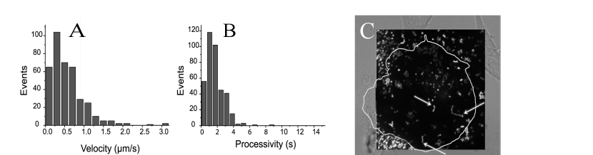
Figure 5: Histograms of the speed (A) and processivity (B) of kinesin in Hela cells. The results confirmed in vitro measurements. (C) Picture of the trajectories (arrows) of a QD labeled Kinesins: image obtained choosing the maximal intensity over many frames of a movie with long integration time (100ms).

V Conclusion

In this proceeding we have reviewed a model introduced to describe intracellular transport parmeggiani-franosch-frey:03 and its possible extensions towards a more realistic picture: we investigated how the introduction of dimers pierobon-frey-franosch:06 and the presence of disorder on the track pierobon-etal:06 would affect the known results. These theoretical approaches while aiming to a realistic description of the traffic phenomena, are inspiring statistical models interesting in its own right (see e.g. chowdhury-schadschneider-nishinari:05 ; mobilia-etal:06 ). The latest experimental successes in tracking individual motors in living cells combined with an appropriate analysis, presented in the last section, could not only confirm the theories but also provide ispiration for a complete picture of the cell logistic.

Acknowledgments

I would like to thank the coauthors of Refs.pierobon-frey-franosch:06 ; pierobon-etal:06 ; cappello-etal:07 . I benefit from useful discussions with A. Parmeggiani, S. Achouri, A. Dunn and L. Sengmanivong.

References

- (1) B. Alberts, A. Johnson, J. Lewis, M. Raff, K. Roberts, and P. Walter. Molecular Biology of the Cell. Garland Science, New York, NY, USA, 4th edition, 2002.
- (2) J. Howard. Mechanics of motor proteins and the cytoskeleton. Sinauer Associates, Inc., Sunderland, MA, USA, 2001.
- (3) C.T. MacDonald, J.H. Gibbs, and A.C. Pipkin. Biopolymers, 6:1–25, 1968.
- (4) B. Derrida, E. Domany, and D. Mukamel. J. Stat. Phys., 69:667–687, 1992.
- (5) G. Schütz and E. Domany. J. Stat. Phys., 72:277–296, 1993.
- (6) A. Parmeggiani, T. Franosch, and E. Frey. Phys. Rev. Lett., 90:086601, 2003.
- (7) A. Parmeggiani, T. Franosch, and E. Frey. Phys. Rev. E, 70:046101, 2004.
- (8) P. Pierobon, T. Franosch, and E. Frey. Phys. Rev. E, 74(031920), 2006.
- (9) T. Chou and G. Lakatos. Phys. Rev. Lett., 93:19, 2004.
- (10) L.B. Shaw, R.K.P. Zia, and K.H. Lee. Phys. Rev. E, 68:021910, 2003.
- (11) J.D. McGhee and P.H. von Hippel. J. Mol. Biol., 86:469–489, 1974.
- (12) E. Frey and A. Vilfan. Chemical Physics, 284:287–310, 2002.
- (13) R.J. Harris and R.B. Stinchcombe. Phys. Rev. E, 70:016108, 2004.
- (14) R. Juhász, L. Santen, and F. Iglói. Phys. Rev. Lett., 94:010601, 2005.
- (15) K.M. Kolwankar and A. Punnoose. Phys. Rev. E, 61(3/4):2453–2456, 2000.
- (16) P. Pierobon, M. Mobilia, R. Kouyos, and E. Frey. Phys. Rev. E, 74(031906), 2006.
- (17) A. B. Kolomeisky. J. Phys. A, 31:1152–1164, 1998.
- (18) L. B. Shaw, A. B. Kolomeisky, and K. H. Lee. J. Phys. A, 37:2105–2113, 2004.
- (19) P. Pierobon. PhD thesis, Ludwig Maximilian Universität München, 2006.
- (20) B. Derrida, M.R. Evans, and D. Mukamel. J. Phys. A, 26:4911–4918, 1993.
- (21) C. Veigel, F. Wang, M. L. Bartoo, J. R. Sellers, and J. E. Molloy. Nat. Cell. Biol., 4:59, 2002.
- (22) S. Uemura, H. Higuchi, A. O. Olivares, E. M. De La Cruz, and S. Ishiwata. Nat Struct. and Mol. Biol., 11:877, 2004.
- (23) A. R. Dunn and J. A. Spudich. Nat. Struct. Mol. Biol., 14:246–8, 2007.
- (24) G. Cappello, P. Pierobon, C. Symonds, L. Busoni, C. Gebhardt, M. Rief, and J. Prost. Proc. Natl. Acad. Sci. USA, 104(39):15328–15333, 2007.
- (25) A. Seitz and T. Surrey. The EMBO Journal, 25(2):267–77, 2006.
- (26) M. Dahan, S. Lévi, C. Luccardini, P. Rostaing, B. Riveau, and A. Triller. Science, 302:302, 2003.
- (27) C. Kural, H. Kim, S. Syed, G. Goshima, V.I. Gelfand, and P.R. Selvin. Science, 308:1469–1472, 2005.
- (28) X.S. Xie, J. Yu, and W.Y. Yang. Science, 312:228, 2006.
- (29) T.M. Watanabe and H. Higuchi. Biophys. J., 92(11):4109–4120, 2007.
- (30) S. Courty, C. Luccardini, Y. Bellaiche, G. Cappello, and M. Dahan. Nanoletters, 6:1491–1945, 2006.
- (31) A. Yildiz, J. N. Forkey, S. A. McKinney, T. Ha, Y. E. Goldman, and P. R. Selvin. Science, 300:2061–5, 2003.
- (32) D. Chowdhury, A. Schadschneider, and K. Nishinari. Physics of Life reviews, 2:318–352, 2005.
- (33) M. Mobilia, T. Reichenbach, H. Hinsch, T. Franosch, and E. Frey. arxiv:cond-mat/0612516, 2006.