Top Hypercharge

Abstract:

We propose a top hypercharge model with gauge symmetry $SU(3)_{C}\times SU(2)_{L}\times U(1)_{1}\times U(1)_{2}$ where the first two families of the Standard Model (SM) fermions are charged under $U(1)_{1}$ while the third family is charged under $U(1)_{2}$. The $U(1)_{1}\times U(1)_{2}$ gauge symmetry is broken down to the $U(1)_{Y}$ gauge symmetry, when a SM singlet Higgs field acquires a vacuum expectation value. We consider the electroweak constraints, and compare the fit to experimental observables to that of the SM. We study the quark CKM mixing between the first two families and the third family, the neutrino masses and mixing, the flavour changing neutral current effects in meson mixing and decays, the $Z^{\prime}$ discovery potential at the Large Hadron Collider, the dark matter with a gauged $Z_{2}$ symmetry, and the Higgs boson masses.

1 Introduction

There are many motivations for physics beyond the Standard Model (SM). For example, the fine-tuning problem such as the gauge hierarchy problem leads to supersymmetry [1], technicolor [2], extra dimensions [3, 4], and other models. Aesthetic considerations such as the unification of the fundamental interactions and the explanation of the charge quantization lead to Grand Unified Theories (GUTs) [5] and string theory [6, 7]. In this paper, we choose to neglect the fine-tuning and aesthetic concerns, and concentrate on the electroweak precision measurements from a phenomenological point of view.

As we learn from the particle data book, there are four measurements with significant deviations: $\sigma_{\rm had}$, $A_{FB}^{(0,b)}$, $A_{e}$ and $g_{L}^{2}$ have $2.0$ $\sigma$, $-2.4$ $\sigma$, $2.0$ $\sigma$, and $-2.7$ $\sigma$ deviations (pull from experimental values), respectively [8]. A simple solution to such deviations is a $U(1)^{\prime}$ model where an additional $U(1)^{\prime}$ gauge symmetry is introduced [9]. Moreover, the masses of the third family fermions are relatively larger than those of the first two families. The quark CKM mixings between the first two families and the third family are small while the neutrino mixings are bilarge. These facts may imply that the first two families and the third family may have different $U(1)^{\prime}$ charges, and the right-handed neutrinos might be neutral under $U(1)^{\prime}$ so that the seesaw mechanism still works [10]. To avoid the introduction of a global symmetry which can be broken via quantum gravity effects, the model may contain a gauged $Z_{2}$ symmetry, and a field charged odd under the symmetry can be a dark matter candidate. Interestingly, the additional $U(1)^{\prime}$ symmetry can easily generate the required gauged $Z_{2}$ symmetry after it is broken. In general, the $U(1)^{\prime}$ model is well motivated from the superstring constructions [11], four-dimensional GUTs [12], higher dimensional orbifold GUTs [13], as well as models with dynamical symmetry breaking [14].

In this paper, we propose a top hypercharge model where the first two families of the SM fermions are charged under $U(1)_{1}$ and the third family is charged under $U(1)_{2}$. We note in passing that top color and top flavour models have been considered in Refs. [15] and [16], respectively. The $U(1)_{1}\times U(1)_{2}$ gauge symmetry is equivalent to the $U(1)_{Y}\times U(1)^{\prime}$ gauge symmetry after an $SO(2)$ rotation of the $U(1)_{1}\times U(1)_{2}$ gauge fields. The $U(1)_{1}\times U(1)_{2}$ gauge symmetry is broken down to the $U(1)_{Y}$ by giving a vacuum expectation value (VEV) to a SM singlet Higgs field. The $SU(2)_{L}\times U(1)_{Y}$ gauge symmetry is further broken down to the electromagnetic $U(1)_{EM}$ gauge symmetry by giving VEV’s to SM doublets. We calculate the neutral gauge boson masses and their corresponding mass eigenstates, and the charged gauge boson masses. Moreover, we consider electroweak constraints, and perform a $\chi^{2}$ analysis for various experimental observables. Our model achieves a better fit than the SM. To generate the quark CKM mixings between the first two families and the third family, we need to introduce an additional SM Higgs doublet or extra vector-like particles. We consider the flavour-changing neutral current (FCNC) effects in $B$ physics, and obtain the corresponding constraints. In addition, we consider the $Z^{\prime}$ production and its discovery potential at the Large Hadron Collider (LHC), a dark matter candidate with the gauged $Z_{2}$ symmetry, and the Higgs boson masses.

This paper is organized as follows. We present the model in Section 2, consider the electroweak constraints in Section 3, and study the quark CKM mixings and FCNC effects in Section 4. The $Z^{\prime}$ production, dark matter and the Higgs boson masses are discussed in Sections 5 and 6, respectively. Our conclusions are given in Section 7.

2 The model

The top hypercharge model is based on the gauge group $SU(3)_{C}\times SU(2)_{L}\times U(1)_{1}\times U(1)_{2}$. The first two families of the SM fermions are charged under $U(1)_{1}$ while the third family is charged under $U(1)_{2}$. The $U(1)_{1}\times U(1)_{2}$ gauge symmetry is equivalent to the $U(1)_{Y}\times U(1)^{\prime}$ gauge symmetry after an $SO(2)$ rotation of the gauge fields. The representations of the SM fermions under the $SU(3)_{C}\times SU(2)_{L}\times U(1)_{1}\times U(1)_{2}$ gauge symmetry are as follows

$$Q_{iL}:(3,2,~{}1/6,~{}0)~{},\hskip 28.45274ptQ_{3L}:(3,2,~{}0,~{}1/6)~{},$$

$$u_{iR}:(3,1,~{}2/3,~{}0)~{},\hskip 28.45274ptu_{3R}:(3,1,~{}0,~{}2/3)~{},$$

$$d_{iR}:(3,1,~{}-1/3,~{}0)~{},\hskip 28.45274ptd_{3R}:(3,1,~{}0,~{}-1/3)~{},$$

$$L_{iL}:(1,2,~{}-1/2,~{}0)~{},\hskip 28.45274ptL_{3L}:(1,2,~{}0,~{}-1/2)~{},$$

$$e_{iR}:(1,1,~{}-1,~{}0)~{},\hskip 28.45274pte_{3R}:(1,1,~{}0,~{}-1)~{},$$

$$N_{k}:(1,1,~{}0,~{}0)~{},~{}\,$$ (1)

where $i=1,2$, and $k=1,2,3$. $Q$ and $L$ denote the left-handed $SU(2)_{L}$ doublets of quarks and leptons, respectively. $u$, $d$, $N$, and $e$ denote the right-handed up-type quark, down-type quark, right-handed neutrino, and charged lepton, respectively. The right-handed neutrinos $N_{k}$ with intermediate-scale masses are included to account for the neutrino masses and mixings via the seesaw mechanism [10]. With the right-handed neutrinos, it is possible to generate baryon asymmetry via leptogenesis [17].

The covariant derivative is written as

$$D_{\mu} = \partial_{\mu}-igA^{a}_{\mu}T^{a}-ig^{\prime}_{1}B^{1}_{\mu}Y_{1}-ig^{\prime}_{2}B^{2}_{\mu}Y_{2}\ ,$$ (2)

where $T^{a}$ are the $SU(2)_{L}$ generators, and $Y_{1(2)}$ is the $U(1)_{1(2)}$ charge of the corresponding particle. In addition, $A^{a}$ and $B^{1(2)}$ are respectively the gauge bosons for $SU(2)_{L}$ and $U(1)_{1(2)}$ gauge symmetries with the coupling constants $g$ and $g^{\prime}_{1(2)}$.

The $SU(3)_{C}\times SU(2)_{L}\times U(1)_{1}\times U(1)_{2}$ symmetry needs to be broken down to the SM gauge symmetry. It is accomplished by the VEV of a complex scalar field $\Sigma$ , which transforms as $(1,1,1/2,-1/2)$. The relevant term in the Lagrangian is $(D_{\mu}\Sigma)^{\dagger}(D^{\mu}\Sigma)$. We set $\langle\Sigma\rangle=u/\sqrt{2}$, then the gauge fields $B^{1}_{\mu}$ and $B^{2}_{\mu}$ acquire a mass-squared matrix

$$\frac{u^{2}}{4}\left(\begin{array}[]{cc}{g^{\prime}_{1}}^{2}&-g^{\prime}_{1}g^{\prime}_{2}\\ -g^{\prime}_{1}g^{\prime}_{2}&{g^{\prime}_{2}}^{2}\\ \end{array}\right)~{}~{}.$$ (5)

At the scale $u$, this renders a massless and a massive gauge bosons

$$B_{\mu} = \cos\phi B^{1}_{\mu}+\sin\phi B^{2}_{\mu}~{},$$

$$\widetilde{B}_{\mu} = -\sin\phi B^{1}_{\mu}+\cos\phi B^{2}_{\mu}~{},$$ (6)

where the mixing angle $\phi$ is defined by $\tan\phi=g^{\prime}_{1}/g^{\prime}_{2}$, with the corresponding masses

$$m^{2}_{B_{\mu}}=0~{},\hskip 28.45274ptm^{2}_{\widetilde{B}_{\mu}}={1\over 4}({g^{\prime}_{1}}^{2}+{g^{\prime}_{2}}^{2})u^{2}~{}.$$ (7)

The massless field $B_{\mu}$ corresponds to the hypercharge gauge field in the SM.

Using the inverse transformation, we write the covariant derivative in terms of $B_{\mu}$ and $\widetilde{B}_{\mu}$ as

$$D_{\mu}= \partial_{\mu}-igA^{a}_{\mu}T^{a}-ig^{\prime}(Y_{1}+Y_{2})B_{\mu}-ig^{\prime}(-Y_{1}\tan\phi+Y_{2}\cot\phi)\widetilde{B}_{\mu}~{},$$ (8)

where

$$Y=Y_{1}+Y_{2}~{},~{}~{}\frac{1}{g^{\prime 2}}=\frac{1}{g_{1}^{\prime 2}}+\frac{1}{g_{2}^{\prime 2}}~{}.~{}\,$$ (9)

In terms of the electron charge $e$, the analog of the weak mixing angle $\theta$ in the SM, and the $SO(2)$ rotation angle $\phi$, we can express the three coupling constants in the model as

$$g=\frac{e}{\sin\theta}~{},\hskip 14.22636ptg^{\prime}_{1}=\frac{e}{\cos\theta\cos\phi}~{},\hskip 14.22636ptg^{\prime}_{2}=\frac{e}{\cos\theta\sin\phi}~{}.$$ (10)

Now we introduce two scalar Higgs doublets $\Phi_{1}$ and $\Phi_{2}$, which transform under $SU(3)_{C}\times SU(2)_{L}\times U(1)_{1}\times U(1)_{2}$ as $(1,2,1/2,0)$ and $(1,2,0,1/2)$. When they acquire the following VEVs

$$\langle\Phi_{1}\rangle={1\over\sqrt{2}}\left(\begin{array}[]{c}0\\ v_{1}\end{array}\right)~{},~{}~{}~{}~{}~{}\langle\Phi_{2}\rangle={1\over\sqrt{2}}\left(\begin{array}[]{c}0\\ v_{2}\end{array}\right)~{},$$ (15)

the $SU(2)_{L}\times U(1)_{Y}$ gauge symmetry is broken down to the $U(1)_{EM}$. $\Phi_{1}$ is responsible for the masses of the fermions of the first two generations, and $\Phi_{2}$ the third generation. As the hierarchy in the fermion mass spectrum indicates, one expects that $v_{1}$ may be smaller than $v_{2}$. And we define

$$\tan\beta\equiv{{v_{2}}\over{v_{1}}}~{}.~{}\,$$ (16)

The terms $(D_{\mu}\Phi_{1})^{\dagger}(D^{\mu}\Phi_{1})+(D_{\mu}\Phi_{2})^{\dagger}(D^{\mu}\Phi_{2})$ in the Lagrangian lead to the following mass terms for the $SU(2)_{L}\times U(1)_{1}\times U(1)_{2}$ gauge bosons after $\Phi_{1}$ and $\Phi_{2}$ get VEVs

$$\Delta{\cal L} = {1\over 4}g^{2}\left(v_{1}^{2}+v_{2}^{2}\right)W^{+}_{\mu}W^{-\mu}$$ (24)

$$+ {1\over 8}\left(\begin{array}[]{ccc}B_{\mu}^{1}&B_{\mu}^{2}&A_{\mu}^{3}\end{array}\right)\left(\begin{array}[]{ccc}{g_{1}^{\prime}}^{2}v_{1}^{2}&0&-gg_{1}^{\prime}v_{1}^{2}\\ 0&{g_{2}^{\prime}}^{2}v_{2}^{2}&-g{g_{2}^{\prime}}^{2}v_{2}^{2}\\ -gg_{1}^{\prime}v_{1}^{2}&-gg_{2}^{\prime}v_{2}^{2}&g^{2}(v_{1}^{2}+v_{2}^{2})\end{array}\right)\left(\begin{array}[]{c}B^{1\mu}\\ B^{2\mu}\\ A^{3\mu}\end{array}\right)~{}.$$

Therefore, the $W$ bosons get mass $m^{2}_{W}={1\over 4}g^{2}(v_{1}^{2}+v_{2}^{2})$, and the mass-squared matrix of the neutral gauge sector becomes

$$M_{neutral}^{2}=\frac{u^{2}}{4}\left(\begin{array}[]{ccc}{g^{\prime}_{1}}^{2}(1+\epsilon_{1})&-g_{1}^{\prime}g_{2}^{\prime}&-gg_{1}^{\prime}\epsilon_{1}\\ -g_{1}^{\prime}g_{2}^{\prime}&{g^{\prime}_{2}}^{2}(1+\epsilon_{2})&-gg^{\prime}_{2}\epsilon_{2}\\ -gg_{1}^{\prime}\epsilon_{1}&-gg_{2}^{\prime}\epsilon_{2}&g^{2}(\epsilon_{1}+\epsilon_{2})\end{array}\right)~{},$$ (28)

where $\epsilon_{1}\equiv v_{1}^{2}/u^{2}$ and $\epsilon_{2}\equiv v_{2}^{2}/u^{2}$, and the basis is $(B^{1}_{\mu},~{}B^{2}_{\mu},~{}A^{3}_{\mu})$. The matrix can be diagonalized by an orthogonal matrix $R$

$$R^{T}M_{neutral}^{2}R={\rm diag}\{0,~{}m_{Z}^{2},~{}m_{Z^{\prime}}^{2}\}~{},$$ (29)

where 0, $m_{Z}^{2}$ and $m_{Z^{\prime}}^{2}$ are the eigenvalues of $M_{neutral}^{2}$. The 0 eigenvalue corresponds to the massless photon field $A_{\mu}$, and the other two non-zero eigenvalues correspond to $Z$ and $Z^{\prime}$ gauge bosons. We use $Z$ to denote the “light $Z$ boson”, which is the observed one, and $Z^{\prime}$ to denote the “heavy $Z$ boson”. The transformation between the weak eigenstates and mass eigenstates is

$$\left(\begin{array}[]{c}B_{\mu}^{1}\\ B_{\mu}^{2}\\ A_{\mu}^{3}\end{array}\right)=R\left(\begin{array}[]{c}A_{\mu}\\ Z_{\mu}\\ Z_{\mu}^{\prime}\end{array}\right)~{}.$$ (36)

To obtain the interactions between the SM fermions and gauge bosons, we write the covariant derivative in terms of the mass eigenstates of gauge bosons

$$D_{\mu} = \partial_{\mu}-i{g\over\sqrt{2}}\left(T^{+}W^{+}_{\mu}+T^{-}W^{-}_{\mu}\right)$$ (37)

$$- i\left(gT_{3}R_{32}+g_{1}^{\prime}Y_{1}R_{12}+g_{2}^{\prime}Y_{2}R_{22}\right)Z_{\mu}$$

$$- i\left(gT_{3}R_{33}+g_{1}^{\prime}Y_{1}R_{13}+g_{2}^{\prime}Y_{2}R_{23}\right)Z^{\prime}_{\mu}$$

$$- ieQA_{\mu}~{},$$

where $T^{\pm}=(T^{1}\pm iT^{2})$, and $Q=T_{3}+Y=T_{3}+Y_{1}+Y_{2}$ is the electric charge for the corresponding particle.

The Lagrangian of the SM fermion Yukawa couplings is

$$-{\cal L}_{Yukawa} = Y^{u}_{i}\bar{u}_{iR}\Phi_{1}Q_{iL}+Y^{u}_{3}\bar{u}_{3R}\Phi_{2}Q_{3L}+Y^{d}_{ij}\bar{d}_{iR}\widetilde{\Phi}_{1}Q_{jL}+Y^{d}_{33}\bar{d}_{3R}\widetilde{\Phi}_{2}Q_{3L}$$ (38)

$$+ Y^{e}_{i}\bar{e}_{iR}\widetilde{\Phi}_{1}L_{iL}+Y^{e}_{3}\bar{e}_{3R}\widetilde{\Phi}_{2}L_{3L}+Y^{\nu}_{ki}N_{k}\Phi_{1}L_{i}+Y^{\nu}_{k3}N_{k}\Phi_{2}{L}_{3}$$

$$+ M_{kl}^{N}N_{k}N_{l}+h.c.~{},$$

where $i,j=1,2$, $k,l=1,2,3$, and $\widetilde{\Phi}=i\sigma_{2}\Phi^{*}$. In the presence of $\Phi_{1}$ and $\Phi_{2}$, there will be Yukawa mixings between the first two generations only, for both quarks and leptons. Interestingly, there is no problem for the neutrino mixings. The point is that after the seesaw mechanism [10], the bilarge neutrino mixings can be mainly generated from the neutrino sector via the mixings in the right-handed Majorana neutrino mass matrix $M_{kl}^{N}$. In fact, after the seesaw mechanism, we obtain the following dimension-5 operators

$$-{\cal L}={{\Phi_{1}L_{i}\Phi_{1}L_{j}}\over{\Lambda_{ij}}}+{{\Phi_{1}L_{i}\Phi_{2}L_{3}}\over{\Lambda_{i3}}}+{{\Phi_{2}L_{3}\Phi_{2}L_{3}}\over{\Lambda_{33}}}~{},~{}\,$$ (39)

where $\Lambda_{ij}$, $\Lambda_{i3}$, and $\Lambda_{33}$ are intermediate mass scales related to the right-handed neutrino masses. Moreover, the SM quark CKM mixings can be generated by introducing extra Higgs doublets or heavy vector-like fermions, which will be discussed in Section 4.

3 Electroweak constraints

The model contains a new gauge boson $Z^{\prime}$, the mass of which can be constrained by the electroweak observables. We calculate in our model the predicted values of the observables in the $\overline{MS}$ scheme, as used in Ref. [8]. For all observables, we compute the deviations from the SM at the tree level and then scale them by the same loop corrections as in the SM, which are given in Table 10.1 of Ref. [8]. The value of $\sin^{2}\theta$ in the $\overline{MS}$ scheme is $\approx 0.2312$ for the SM. In our model, it receives a correction in order to reproduce the correct $Z$ mass. Other inputs used here are $\hat{\alpha}(M_{Z})^{-1}=127.904$ and $v=246.3$ GeV.

In the model, the first two generations of fermions couple to the regular $Z$ boson differently from the third one. Therefore, if there is mixing between these generations, there can be FCNC at the tree level. However, this is not seen to happen since the branching ratios of the corresponding $Z$ decay modes are very small. For example, we have the experimental bounds [8] $BR(Z\to e^{\pm}\mu^{\mp})<1.7\times 10^{-6}$, $BR(Z\to e^{\pm}\tau^{\mp})<9.8\times 10^{-6}$ and $BR(Z\to\mu^{\pm}\tau^{\mp})<1.2\times 10^{-5}$ at 95% confidence level (CL). There is also no evidence that the $Z$ boson decays to quark pairs of different flavors. Therefore, in the calculation of $Z$ pole observables, we avoid considering $Z$-mediated FCNC.

The electroweak precision bounds can be consistent with our model predictions as long as $\epsilon_{1}$ and $\epsilon_{2}$ are taken to be very small. However, if $\epsilon_{1}$ and $\epsilon_{2}$ are very small, the mass of $Z^{\prime}$ will be so large that it is beyond the LHC reach in the near future. Therefore, we will concentrate on the parameter space where $M_{Z^{\prime}}$ is in the a few TeV range. In this section, for completeness, we will perform the analysis by choosing $\tan\beta\equiv v_{2}/v_{1}$ equal to 0.5, 1, 2, 5, 10, 20, 35 and 50. We emphasize that if $\tan\beta$ is small than 1, there exists the Landau pole problem for the top quark Yukawa coupling below the grand unification scale, string scale or Planck scale. However, the Landau pole problem can be solved if the cut-off scale or the fundamental scale is low, for example, the large extra dimensions [3]. In addition, it is more natural to take $\tan\beta>1$, hence, we will concentrate on it when we study the phenomenological consequences of our model in the following sections.

Table 1: The experimental [8] and the predicted values of the $Z$-pole observables for the SM [8] and our model with $\tan\beta$=2 and 50 as two examples. For best fits, the $\tan\beta=2$ case has $\cos^{2}\phi=4.3$ and $M_{Z^{\prime}}=2.4$ TeV, and the $\tan\beta=50$ case has $\cos^{2}\phi=1.22$ and $M_{Z^{\prime}}=10$ TeV.

Observables	Experimental data	SM		$\tan\beta=2$		$\tan\beta=50$
		best fit	pull	best fit	pull	best fit	pull
$M_{W}({\rm GeV})$	$80.450\pm 0.058$	$80.376$	$1.3$	$80.376$	$1.3$	$80.376$	$1.3$
$\Gamma_{Z}({\rm TeV})$	$2.4952\pm 0.0023$	$2.4968$	$-0.7$	$2.4972$	$-0.9$	$2.4971$	$-0.8$
$\sigma_{\rm had}[nb]$	$41.541\pm 0.037$	$41.467$	$2.0$	$41.477$	$1.7$	$41.470$	$1.9$
$R_{e}$	$20.804\pm 0.050$	$20.756$	$1.0$	$20.7498$	$1.1$	$20.7534$	$1.0$
$R_{\mu}$	$20.785\pm 0.033$	$20.756$	$0.9$	$20.7498$	$1.1$	$20.7534$	$1.0$
$R_{\tau}$	$20.764\pm 0.045$	$20.801$	$-0.8$	$20.8110$	$-1.0$	$20.8035$	$-0.9$
$R_{b}$	$0.21629\pm 0.00066$	$0.21578$	$0.8$	$0.21570$	$0.9$	$0.21576$	$0.8$
$R_{c}$	$0.1721\pm 0.0030$	$0.17230$	$-0.1$	$0.17231$	$-0.1$	$0.17230$	$-0.1$
$A_{e}$	$0.15138\pm 0.00216$	$0.1471$	$2.0$	$0.1454$	$2.8$	$0.1463$	$2.4$
$A_{\mu}$	$0.142\pm 0.015$	$0.1471$	$-0.3$	$0.1454$	$-0.2$	$0.1463$	$-0.3$
$A_{\tau}$	$0.136\pm 0.015$	$0.1471$	$-0.7$	$0.1484$	$-0.8$	$0.1472$	$-0.7$
$A_{b}$	$0.923\pm 0.020$	$0.9347$	$-0.6$	$0.9348$	$-0.6$	$0.9347$	$-0.6$
$A_{c}$	$0.670\pm 0.027$	$0.6678$	$0.1$	$0.6670$	$0.1$	$0.6674$	$0.1$
$A_{s}$	$0.895\pm 0.091$	$0.9356$	$-0.4$	$0.9355$	$-0.4$	$0.9355$	$-0.4$
$A^{e}_{FB}$	$0.0145\pm 0.0025$	$0.01622$	$-0.7$	$0.01584$	$-0.5$	$0.01604$	$-0.6$
$A^{\mu}_{FB}$	$0.0169\pm 0.0013$	$0.01622$	$0.5$	$0.01584$	$0.8$	$0.01604$	$0.7$
$A^{\tau}_{FB}$	$0.0188\pm 0.0017$	$0.01622$	$1.5$	$0.01617$	$1.5$	$0.01614$	$1.6$
$A^{b}_{FB}$	$0.0992\pm 0.0016$	$0.1031$	$-2.4$	$0.1019$	$-1.7$	$0.1025$	$-2.1$
$A^{c}_{FB}$	$0.0707\pm 0.0035$	$0.0737$	$-0.8$	$0.0728$	$-0.6$	$0.0732$	$-0.7$
$A^{s}_{FB}$	$0.0976\pm 0.0114$	$0.1032$	$-0.5$	$0.1020$	$-0.4$	$0.1026$	$-0.4$
$g_{L}^{2}$	$0.30005\pm 0.00137$	$0.30378$	$-2.7$	$0.30398$	$-2.9$	$0.30390$	$-2.8$
$g_{R}^{2}$	$0.03076\pm 0.00110$	$0.03006$	$0.6$	$0.03034$	$0.4$	$0.03037$	$0.4$
$g_{V}^{\nu e}$	$-0.040\pm 0.015$	$-0.03936$	$0.0$	$-0.03804$	$-0.1$	$-0.03780$	$-0.1$
$g_{A}^{\nu e}$	$0.507\pm 0.014$	$-0.5064$	$0.0$	$-0.5071$	$0.0$	$-0.5071$	$0.0$

We scan the parameter space for $M_{Z^{\prime}}<10$ TeV, and obtain the allowed deviation at 3$\sigma$ level of the observables including $M_{W}$, $\Gamma_{Z}$, $R_{(e,\mu,\tau,b,c)}$, $\sigma_{had}$, $A^{FB}_{(e,\mu,\tau,c,b,s)}$, $A_{(e,\mu,\tau,b,c,s)}$, $g_{(L,R)}^{2}$ and $g_{(V,A)}^{\nu e}$. In the allowed region, we get the $\chi^{2}$ values of every points, and then divide the regions into five sub-regions according to $\chi^{2}$, they are $\chi^{2}<32$, $32<\chi^{2}<33$, $33<\chi^{2}<34$, $34<\chi^{2}<35$ and $\chi^{2}>35$. This is shown in Fig. 1. When $\tan\beta$ is 0.5 and 1, $M_{Z^{\prime}}$ can be as low as less than $500$ GeV. But as mentioned before, we will concentrate exclusively on the region where $M_{Z^{\prime}}$ is larger than 1 TeV. Since the $\chi^{2}$ value for the SM is 32.01, so the blue regions can be regarded as the regions where our model has a better fit than the SM. Besides the blue areas, there are still large regions equally consistent with the current weak scale experiments as the SM. The minimal $\chi^{2}$ values in the allowed regions for $\tan\beta=0.5,1,2,5,10,20,35,50$ are 31.82, 31.89, 31.88, 31.87, 31.90, 31.92, 31.92 and 31.92, respectively. To be concrete, we present the experimental [8] and predicted values of the $Z$-pole observables for the SM [8] and our model with $\tan\beta$=2 and 50 for the best fits in Table 1.

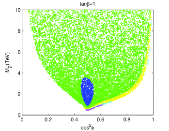
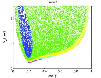
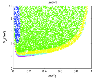
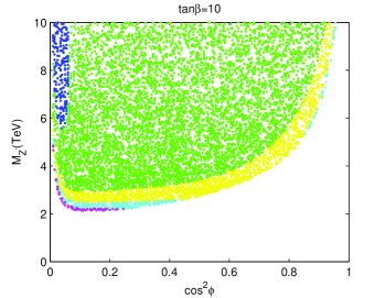
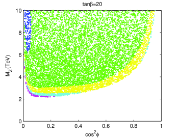
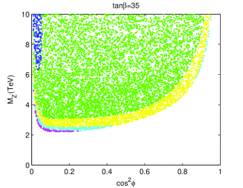
Figure 1: Allowed regions of the parameter space for various $\tan\beta$. In all figures, the colors denote regions with different $\chi^{2}$ ranges, blue: $\chi^{2}<32$, green: $32<\chi^{2}<33$, yellow: $33<\chi^{2}<34$, cyan: $34<\chi^{2}<35$, magenta: $\chi^{2}>35$.

The gauge group of the model can be regarded as $SU(3)_{C}\times SU(2)_{L}\times U(1)_{Y}\times U(1)^{\prime}$, where the gauge bosons of $U(1)_{Y}$ and $U(1)^{\prime}$ are $B_{\mu}$ and $\widetilde{B}_{\mu}$, as given in Eq. (6). In general there is a mixing between $Z$ and $Z^{\prime}$, and the mixing angle is constrained to be $10^{-3}$ or smaller [8]. In our model, this is achieved when $M_{Z^{\prime}}$ is larger than $1$ TeV. Interestingly, we note that when $\tan\phi=\tan\beta$, there is no mixing between $Z$ and $Z^{\prime}$, and then the electroweak precision constraints can be relaxed as well.

4 Quark mixing and FCNC

In our model, there are no intrinsic quark Yukawa mixings between the first two families and the third family. These mixings can be generated by introducing additional Higgs doublet fields $\Phi_{3}$, $\Phi_{4}$, $\Phi_{5}$, and $\Phi_{6}$ with quantum numbers $(1,2,-1/6,-1/3)$, $(1,2,-1/3,-1/6)$, $(1,2,-1/6,2/3)$, and $(1,2,2/3,-1/6)$, respectively. If we introduce the Higgs doublet fields $\Phi_{3}$ and $\Phi_{4}$, the quark CKM mixings can arise from the down-type quark mass matrix from the following Yukawa couplings

$$-{\cal L}_{Yukawa} = Y^{d}_{3i}\bar{d}_{3R}\Phi_{3}Q_{iL}+Y^{d}_{i3}\bar{d}_{iR}\Phi_{4}Q_{3L}+h.c.~{}.~{}\,$$ (40)

Even if we merely introduce $\Phi_{3}$ or $\Phi_{4}$, we can still generate the quark CKM mixings by choosing suitable Yukawa couplings. Similarly, if we introduce the Higgs doublet fields $\Phi_{5}$ and $\Phi_{6}$, the quark CKM mixings can arise from up-type quark mass matrix.

Without adding extra Higgs doublet fields, we can also generate the quark CKM mixings by introducing additional Higgs singlet field and heavy vector-like fields. For example, we introduce a SM singlet Higgs field $S$ with quantum numbers $(1,1,-1/6,1/6)$, and vector-like fields ($Q_{X}$, $\overline{Q}_{X}$), and ($Q^{\prime}_{X}$, $\overline{Q}^{\prime}_{X}$) with the following quantum numbers

$$Q_{X}:(3,2,~{}1/6,~{}0)~{},\hskip 28.45274pt\overline{Q}_{X}:(\bar{3},2,-1/6,~{}0)~{},$$

$${Q}^{\prime}_{X}:(3,2,~{}0,~{}1/6)~{},\hskip 28.45274pt\overline{Q}^{\prime}_{X}:(\bar{3},2,~{}0,-1/6)~{}.$$ (41)

There are new Yukawa coupling terms as the following

$$-{\cal L}_{Yukawa} = y_{XQ}^{i}S\overline{Q}^{\prime}_{X}Q_{i}+y_{XQ}^{3}S^{\dagger}\overline{Q}_{X}Q_{3}+y_{Xu}^{i}\bar{u}_{iR}\Phi_{1}Q_{X}+y_{Xu}^{3}\bar{u}_{3R}\Phi_{2}Q_{X}^{\prime}$$ (42)

$$+ y_{Xd}^{i}\bar{d}_{iR}\widetilde{\Phi}_{1}Q_{X}+y_{Xd}^{3}\bar{d}_{3R}\widetilde{\Phi}_{2}Q_{X}^{\prime}+M_{X}\overline{Q}_{X}Q_{X}+M_{X}^{\prime}\overline{Q}^{\prime}_{X}Q^{\prime}_{X}+h.c.~{},$$

where the masses $M_{X}$ and $M_{X}^{\prime}$ can be generated by introducing another SM singlet Higgs field. For simplicity, we neglect the mixings between $Q_{X}$ and $Q_{iL}$, and between $Q_{X}^{\prime}$ and $Q_{3L}$. After we integrate out the vector-like fields ($Q_{X}$, $\overline{Q}_{X}$) and ($Q^{\prime}_{X}$, $\overline{Q}^{\prime}_{X}$), we obtain

$$-{\cal L}_{Yukawa} = -{1\over{M_{X}}}\left(y_{Xu}^{i}y_{XQ}^{3}\bar{u}_{iR}\Phi_{1}S^{\dagger}Q_{3}+y_{Xd}^{i}y_{XQ}^{3}\bar{d}_{iR}\widetilde{\Phi}_{1}S^{\dagger}Q_{3}\right)$$ (43)

$$- {1\over{M_{X}^{\prime}}}\left(y_{Xu}^{3}y_{XQ}^{i}\bar{u}_{3R}\Phi_{2}SQ_{i}+y_{Xd}^{3}y_{XQ}^{i}\bar{d}_{3R}\widetilde{\Phi}_{2}SQ_{i}\right)+h.c.~{}.~{}\,$$

Thus, we generate the SM quark CKM mixings after $S$ obtains a VEV.

The mismatch between the flavor eigenstates and mass eigenstates of the quarks will result in tree-level flavor-changing $Z^{\prime}$ couplings because the U(1)^′ charges of the third-generation quarks are different from those of the first two generations. We can reduce uncertainties from the up sector by assuming no difference between the flavor and mass eigenstates for the up-type quarks, corresponding to the case where only the $\Phi_{3}$ and $\Phi_{4}$ Higgs fields are introduced, as described above. See, however, Ref. [18] for the situation where the up sector mixings are identical to the CKM mixings, and its consequences to single-top production. In this case, the converting matrix for the down-type quarks is simply the CKM matrix. Following the discussions and notations in Refs. [19, 20], the dominant off-diagonal $Z^{\prime}$ coupling is between the left-handed bottom and strange quarks due to the hierarchical structure in the CKM matrix

$$B_{L}^{sb}=\delta_{L}Q_{d_{L}}V_{tb}V_{ts}^{*}~{},$$ (44)

where the combination

$$\delta_{L}Q_{d_{L}}=\frac{e}{3\sin 2\phi\cos\theta}~{}.$$ (45)

It is interesting to note that there is no $\tan\beta$ dependence in the FCNC coupling $B_{L}^{sb}$. Such a coupling can contribute to processes involving $b\to s$ transitions. In view of their precisions and less theoretical uncertainties, the latest experimental data of the $B_{s}$-$\overline{B}_{s}$ oscillation [21] and $B\to X_{s}\ell^{+}\ell^{-}$ decay [22, 23] are used here to constrain the parameters $\cos\phi$ and $M_{Z^{\prime}}$ appearing in the above expressions.

Given the value $\Delta M_{s}^{\rm exp}=17.77\pm 0.10\pm 0.07$ ps^-1 reported by the CDF Collaboration [21] and the SM expectation $\Delta M_{s}^{\rm SM}=19.52\pm 5.28$ ps^-1, we determine the ratio $\Delta M_{s}^{\rm exp}/\Delta M_{s}^{\rm SM}=0.89\pm 0.24$. Suppose there are only left-handed flavor-changing $Z^{\prime}$ couplings in our model, we find that the allowed parameter space is above the solid curve in Fig. 2. Furthermore, if we assume no mixing in the lepton sector, the constraint given by the $B\to X_{s}\ell^{+}\ell^{-}$ decays renders the space above the dashed green curve. In this case, the $\Delta M_{s}$ constraint is stronger for $Z^{\prime}$ mass above about 500 GeV.

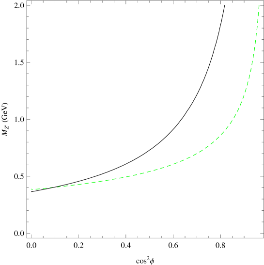
Figure 2: Constraints on the model parameters $(\cos\phi,M_{Z^{\prime}})$ using the $B_{s}$-$\overline{B}_{s}$ oscillation (solid black curve) and the averaged $B\to X_{s}\ell^{+}\ell^{-}$ decay rate (dashed green curve). Here the model only contains the left-handed FCNC couplings for the down quark sector. The allowed parameter space is above the curves.

If there is also a mismatch between the flavor and mass eigenstates for the right-handed quarks, then there will be flavor-changing $Z^{\prime}$ couplings for them and thus additional contributions to the above-mentioned processes. However, such an analysis cannot be done without knowing the mixing information. As an example, if we assume the same CKM matrix for the right-handed quarks, the $Z^{\prime}$-$s_{R}$-$b_{R}$ coupling is

$$B_{R}^{sb}=\delta_{R}Q_{d_{R}}V_{tb}V_{ts}^{*}~{},$$ (46)

where the combination

$$\delta_{R}Q_{d_{R}}=-\frac{2e}{3\sin 2\phi\cos\theta}~{}.$$ (47)

$B_{R}^{sb}$ is also $\tan\beta$ independent. With the inclusion of such flavor-changing $Z^{\prime}$ couplings to both left-handed and right-handed down-type quarks, the allowed parameter space on the $\cos\phi$-$M_{Z^{\prime}}$ plane is given in Fig. 3.

The $B_{s}$-$\overline{B}_{s}$ oscillation data exclude the region below the solid blue curve and the region between the dash-dotted red curves. This slightly more complicated condition results from the introduction of new operators $[\overline{s}\gamma^{\mu}(1-\gamma^{5})b][\overline{s}\gamma_{\mu}(1+\gamma^{5})b]$, $[\overline{s}(1-\gamma^{5})b][\overline{s}(1+\gamma^{5})b]$, and $[\overline{s}\gamma^{\mu}(1+\gamma^{5})b][\overline{s}\gamma_{\mu}(1+\gamma^{5})b]$ in the model. The first two new operators have destructive interference with the third new operator and the standard model operator $[\overline{s}\gamma^{\mu}(1-\gamma^{5})b][\overline{s}\gamma_{\mu}(1-\gamma^{5})b]$. Moreover, the renormalization group running enhances the Wilson coefficient of the former. The $B\to X_{s}\ell^{+}\ell^{-}$ decays in this case has a stronger constraint than the $B_{s}$ mixing when $\cos\phi<0.6$.

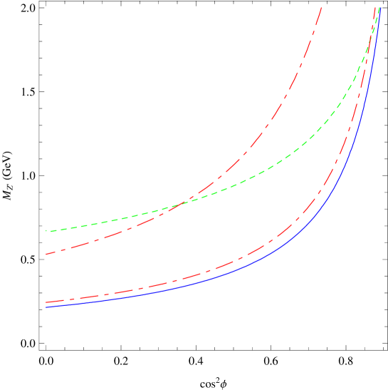
Figure 3: Constraints on the model parameters $(\cos\phi,M_{Z^{\prime}})$ using the $B_{s}$-$\overline{B}_{s}$ oscillation (solid blue and dash-dotted red curves) and the averaged $B\to X_{s}\ell^{+}\ell^{-}$ decay rate (dashed green curve). Here the model contains both the left-handed and right-handed FCNC couplings for the down quark sector. The allowed parameter space is above the solid blue and dashed green curves with the region between the dash-dotted red curves being excluded.

5 $Z^{\prime}$ production

As the previous sections indicate, for a specific choice of $\cos\phi$, $\epsilon_{2}$ is allowed to vary within a certain range while still producing a reasonable fit to the experimental observables. When we consider the $Z^{\prime}$ production at the LHC, we present our results for four values of $\cos\phi$, 0.2, 0.4, 0.6 and 0.8. For each value of $\cos\phi$, $\epsilon_{2}$ is adjusted to generate the corresponding $M_{Z^{\prime}}$ to be within the range of 1 TeV to 5 TeV. Similar to other types of $Z^{\prime}$ models [24], the $Z^{\prime}$ in the top hypercharge model can be searched for through the Drell-Yan processes. For the mass range we consider, the decay width of the $Z^{\prime}$ is typically a few hundred GeV. We apply the simple cuts of requiring the transverse momenta of the outgoing leptons to be larger than 20 GeV, the absolute value of the rapidities of the leptons to be less than 2.5, and the invariant mass of the lepton pair to be between $M_{Z^{\prime}}-1/2\Gamma_{Z^{\prime}}$ and $M_{Z^{\prime}}+1/2\Gamma_{Z^{\prime}}$. After these cuts, the SM background becomes negligible compared to the signal.

We calculate the $pp\to e^{+}e^{-}$ and $\mu^{-}\mu^{+}$ cross sections and deduce the significance for discovery based on the statistical errors. In Fig. 4, we show the total luminosities required for a $5\sigma$ discovery of different $\cos\phi$ and $M_{Z^{\prime}}$ in the top hypercharge model. With 100 fb^-1, the discovery reaches for $\cos\phi=0.8$, 0.6, 0.4 and 0.2 are about 4.1, 5.0, 5.8 and 6.9 TeV, respectively. The production cross sections have a strong dependence on $\cos\phi$, as can be seen in Eq. (37) that the $Z^{\prime}$ coupling to the first two generations of quarks are proportional to $\tan\phi$. Therefore, small $\cos\phi$ will enhance this coupling and large cross sections follow.

Figure 4: The total luminosity required for a 5$\sigma$ discovery through the Drell-Yan process as a function of the $Z^{\prime}$ mass for $\cos\phi=0.2,0.4,0.6$, and $0.8$.

6 Dark matter and Higgs masses

Finally, we comment on the issues of dark matter candidate and Higgs boson masses in this model. As to be seen below, this part of discussions involves more independent parameters. Detailed numerical analyses are beyond the scope of this work and will be presented elsewhere [25].

The dark matter candidate is a particle whose stability can be achieved using an additional discrete symmetry. However, if the discrete symmetry is global but not gauged, this symmetry can be violated by non-renormalizable higher-dimensional operators due to quantum gravity effects. In our model, we can introduce a SM singlet scalar field $\phi$ with quantum number $(1,1,-1/4,1/4)$. The relevant Lagrangian for $\phi$ and its couplings to $\Sigma$ is

$$-{\cal L}_{Yukawa} = m_{\phi}^{2}|\phi|^{2}+{{\lambda_{\phi}}\over 2}|\phi|^{4}+\lambda^{\prime}_{\phi}|\phi|^{2}|\Sigma|^{2}+\left({\widetilde{m}}_{\phi}\phi^{2}\Sigma+h.c.\right)~{}.~{}\,$$ (48)

Thus, after the $U(1)_{1}\times U(1)_{2}$ gauge symmetry is broken down to $U(1)_{Y}$, $\phi$ becomes a stable particle due to the gauged $Z_{2}$ symmetry under which $\phi$ goes to $-\phi$ and the other fields are invariant.

Similar to the singlet-field dark matter [26, 27, 28], $\phi$ can possibly give the correct dark matter density, which deserves further study in details because of the additional $U(1)$ gauge symmetry.

Aside from the above-mentioned $Z_{2}$-odd scalar field, there are at least three Higgs fields in the model, namely $\Sigma$, $\Phi_{1}$ and $\Phi_{2}$. The most general renormalizable Higgs potential is

$$V_{scalar} = -m_{11}^{2}\Phi_{1}^{\dagger}\Phi_{1}-m_{22}^{2}\Phi_{2}^{\dagger}\Phi_{2}-\left[A_{m}\Phi_{1}^{\dagger}\Sigma\Phi_{2}+h.c.\right]$$ (49)

$$+ {1\over 2}\lambda_{1}\left(\Phi_{1}^{\dagger}\Phi_{1}\right)^{2}+{1\over 2}\lambda_{2}\left(\Phi_{2}^{\dagger}\Phi_{2}\right)^{2}+\lambda_{3}\left(\Phi_{1}^{\dagger}\Phi_{1}\right)\left(\Phi_{2}^{\dagger}\Phi_{2}\right)+\lambda_{4}\left(\Phi_{1}^{\dagger}\Phi_{2}\right)\left(\Phi_{2}^{\dagger}\Phi_{1}\right)$$

$$+ \lambda_{5}\left(\Sigma^{\dagger}\Sigma\right)\left(\Phi_{1}^{\dagger}\Phi_{1}\right)+\lambda_{6}\left(\Sigma^{\dagger}\Sigma\right)\left(\Phi_{2}^{\dagger}\Phi_{2}\right)-m_{\Sigma}^{2}\Sigma^{\dagger}\Sigma+{1\over 2}\lambda_{\Sigma}\left(\Sigma^{\dagger}\Sigma\right)^{2}~{},$$

where $A_{m}$ has mass dimension one, and the coefficients $\lambda_{i}$ are real dimensionless quantities. We ignore the possibility of explicit CP-violating effects in the Higgs potential by choosing $A_{m}$ to be real, although in general it can be complex. At the minimum of the potential, we expand the Higgs fields as follows

$$\Sigma={1\over\sqrt{2}}\left(u+\sigma+i\xi\right)~{},~{}\,$$ (50)

$$\Phi_{1}=\left(\begin{array}[]{c}\phi_{1}^{+}\\ {\left(v_{1}+\phi_{1}+i\varphi_{1}\right)/\sqrt{2}}\end{array}\right)~{},~{}~{}\Phi_{2}=\left(\begin{array}[]{c}\phi_{2}^{+}\\ \left(v_{2}+\phi_{2}+i\varphi_{2}\right)/\sqrt{2}\end{array}\right)~{}.$$ (55)

There are ten degrees of freedom in the three Higgs fields. After the $SU(2)_{L}\times U(1)_{1}\times U(1)_{2}$ gauge symmetry is broken down to $U(1)_{EM}$, there will be left with six physical Higgs fields: three CP-even ones ($H_{1}$, $H_{2}$ and $H_{3}$), a CP-odd one ($A$), and a charged pair ($H^{\pm}$). The mass-squared matrix of the CP-even Higgs fields in the basis of $(\sigma,\phi_{1},\phi_{2})$ is

$${\cal M}_{CP-even}^{2}=\left(\begin{array}[]{ccc}{A_{m}v_{1}v_{2}\over\sqrt{2}u}+\lambda_{\Sigma}u^{2}&-{A_{m}v_{2}\over\sqrt{2}}+\lambda_{5}uv_{1}&-{A_{m}v_{1}\over\sqrt{2}}+\lambda_{6}uv_{2}\\ -{A_{m}v_{2}\over\sqrt{2}}+\lambda_{5}uv_{1}&{A_{m}uv_{2}\over\sqrt{2}v1}+\lambda_{1}v_{1}^{2}&-{A_{m}u\over\sqrt{2}}+\left(\lambda_{3}+\lambda_{4}\right)v_{1}v_{2}\\ -{A_{m}v_{1}\over\sqrt{2}}+\lambda_{6}uv_{2}&-{A_{m}u\over\sqrt{2}}+\left(\lambda_{3}+\lambda_{4}\right)v_{1}v_{2}&{A_{m}uv_{1}\over\sqrt{2}v_{2}}+\lambda_{2}v_{2}^{2}\end{array}\right)~{}.$$ (59)

The mass-squared matrix of CP-odd Higgs fields in the basis of $(\xi,\varphi_{1},\varphi_{2})$ is

$${\cal M}_{CP-odd}^{2}=\frac{A_{m}}{\sqrt{2}}\left(\begin{array}[]{ccc}{v_{1}v_{2}u}&-{v_{2}}&{v_{1}}\\ -{v_{2}}&{uv_{2}v_{1}}&-{u}\\ {v_{1}}&-{u}&{uv_{1}v_{2}}\end{array}\right)~{}.$$ (63)

Thus, there are two massless Goldstone bosons and one CP-odd Higgs field $A$ with the following mass

$$m_{A}^{2} = {A_{m}\left(v_{1}^{2}v_{2}^{2}+u^{2}v_{1}^{2}+u^{2}v_{2}^{2}\right)\over\sqrt{2}uv_{1}v_{2}}~{}.$$ (64)

The mass-squared matrix of charged Higgs fields in the basis of $(\phi_{1}^{\pm},~{}\phi_{2}^{\pm})$ is

$${\cal M}_{charged}^{2}=\left(\begin{array}[]{cc}{A_{m}v_{2}u\over\sqrt{2}v_{1}}-{1\over 2}\lambda_{4}v_{2}^{2}&-{A_{m}u\over\sqrt{2}}+{1\over 2}\lambda_{4}v_{1}v_{2}\\ -{A_{m}u\over\sqrt{2}}+{1\over 2}\lambda_{4}v_{1}v_{2}&{A_{m}v_{1}u\over\sqrt{2}v_{2}}-{1\over 2}\lambda_{4}v_{1}^{2}\end{array}\right)~{}.~{}\,$$ (67)

So, we have one pair of massless charged Goldstone bosons, and one pair of charged Higgs bosons with mass

$$m_{H^{\pm}}^{2}={A_{m}u(v_{1}^{2}+v_{2}^{2})\over\sqrt{2}v_{1}v_{2}}-{1\over 2}\lambda_{4}(v_{1}^{2}+v_{2}^{2})~{}.~{}\,$$ (68)

7 Conclusions

In this paper, we proposed a top hypercharge model with the gauge symmetry $SU(3)_{C}\times SU(2)_{L}\times U(1)_{1}\times U(1)_{2}$. The first two families of the SM fermions are charged under $U(1)_{1}$ while the third family is charged under $U(1)_{2}$. We break the $U(1)_{1}\times U(1)_{2}$ gauge symmetry down to the $U(1)_{Y}$ gauge symmetry by giving a VEV to the Higgs field $\Sigma$, which is an $SU(2)_{L}$ singlet but charged under both $U(1)$ groups. We performed a global fit to the electroweak observables at the $Z$-pole in this model and found that in some regions of the parameter space (Fig. 1) the top hypercharge model provides a better fit than the SM. In view of the possibility of a large FCNC associated with the $b\to s$ transition, we studied the constraints by considering the $B_{s}$ mixing and $B\to X_{s}\ell^{+}\ell^{-}$ decays. They generally excluded the regions with $m_{Z^{\prime}}<500$ GeV and large $\cos^{2}\phi$. The production and detection of such a $Z^{\prime}$ boson through the Drell-Yan process at the LHC was calculated for $0.2\leq\cos\phi\leq 0.8$. With an integrated luminosity of $100$ fb^-1, the $5\sigma$ discovery reach ranged from $4.1$ to $6.9$ TeV. We also commented on the possibility that a scalar field charged odd under a gauged $Z_{2}$ symmetry derived from the extra $U(1)$ symmetry may serve as a DM candidate, and the tree-level mass spectrum of the Higgs boson fields. These issues deserve further investigations in the future.

References

- [1] S. Dimopoulos and S. Raby, Nucl. Phys. B 192, 353 (1981); E. Witten, Nucl. Phys. B 188, 513 (1981); M. Dine, W. Fischler and M. Srednicki, Nucl. Phys. B 189, 575 (1981); S. Dimopoulos and H. Georgi, Nucl. Phys. B 193, 150 (1981); N. Sakai, Z. Phys. C 11, 153 (1981); R. K. Kaul and P. Majumdar, Nucl. Phys. B 199, 36 (1982).
- [2] S. Weinberg, Phys. Rev. D 13, 974 (1976); L. Susskind, Phys. Rev. D 20, 2619 (1979);
- [3] N. Arkani-Hamed, S. Dimopoulos and G. R. Dvali, Phys. Lett. B 429, 263 (1998); I. Antoniadis, N. Arkani-Hamed, S. Dimopoulos and G. R. Dvali, Phys. Lett. B 436, 257 (1998);
- [4] L. Randall and R. Sundrum, Phys. Rev. Lett. 83, 3370 (1999); Phys. Rev. Lett. 83, 4690 (1999).
- [5] J. C. Pati and A. Salam, Phys. Rev. D 10, 275 (1974) [Erratum-ibid. D 11, 703 (1975)]; H. Georgi and S. L. Glashow, Phys. Rev. Lett. 32, 438 (1974).
- [6] M. B. Green, J. H. Schwarz and E. Witten, “Superstring Theory”, Vols. 1 and 2 (Cambridge University Press, Cambridge, 1987); and references therein.
- [7] J. Polchinski, “String Theory”, Vols. 1 and 2 (Cambridge University Press, Cambridge, 1998); and references therein.
- [8] W. M. Yao et al. [Particle Data Group], J. Phys. G 33, 1 (2006).
- [9] J. Erler and P. Langacker, Phys. Rev. Lett. 84, 212 (2000).
- [10] T. Yanagida, in Unified Theories, eds. O. Sawada, et al., Feb., 1979; M. Gell-Mann, P. Ramond, R. Slansky, in Sanibel Symposium, CALT-68-709, Feb., 1979, and in Supergravity, eds. D. Freedman, et al. (Amsterdam, 1979); S. L. Glashow, in Quarks and Leptons, Cargese, eds. M. Levy, et al., pp.707, (Plenum, NY, 1980); R. N. Mohapatra and G. Senjanovic, Phys. Rev. Lett. 44, 912 (1980).
- [11] M. Cvetič and P. Langacker, Phys. Rev. D 54, 3570 (1996) and Mod. Phys. Lett. A 11, 1247 (1996).
- [12] For a review, see, M. Cvetič and P. Langacker, in Perspectives on supersymmetry, ed. G. L. Kane (World, Singapore, 1998), p. 312.
- [13] Y. Kawamura, Prog. Theor. Phys. 103, 613 (2000); ibid. 105, 999 (2001); ibid. 105, 691 (2001); G. Altarelli and F. Feruglio, Phys. Lett. B 511, 257 (2001); A. B. Kobakhidze, Phys. Lett. B 514, 131 (2001); L. Hall and Y. Nomura, Phys. Rev. D 64, 055003 (2001); A. Hebecker and J. March-Russell, Nucl. Phys. B 613, 3 (2001); T. Li, Phys. Lett. B 520, 377 (2001); Nucl. Phys. B 619, 75 (2001); I. Gogoladze, Y. Mimura and S. Nandi, Phys. Lett. B 562, 307 (2003); Phys. Rev. Lett. 91, 141801 (2003).
- [14] C. T. Hill and E. H. Simmons, Phys. Rept. 381, 235 (2003) [Erratum-ibid. 390, 553 (2004)].
- [15] C. T. Hill, Phys. Lett. B266, 419 (1991); ibid., B345, 483 (1995); C. T. Hill and S. J. Parke, Phys. Rev. D49, 4454 (1994); D. A. Dicus, B. Dutta, and S. Nandi, Phys. Rev. D51, 6085 (1995).
- [16] X. Li and E. Ma, Phys. Rev. Lett. 47, 1788 (1981); ibid. 60, 495 (1988); Phys. Rev. D46, R1905 (1992); J. Phys. G19, 1265 (1993); R. S. Chivukula, E. H. Simmons, and J. Terning, Phys. Lett. B331, 383 (1994); ibid., Phys. Rev. D53, 5258 (1996); D. J. Muller and S. Nandi, Phys. Lett. B 383, 345 (1996); E. Malkawi, T. Tait and C. P. Yuan, Phys. Lett. B 385, 304 (1996).
- [17] M. Fukugita and T. Yanagida, Phys. Lett. B 174, 45 (1986).
- [18] A. Arhrib, K. Cheung, C. W. Chiang and T. C. Yuan, Phys. Rev. D 73, 075015 (2006).
- [19] V. Barger, C. W. Chiang, P. Langacker and H. S. Lee, Phys. Lett. B 580, 186 (2004) [arXiv:hep-ph/0310073].
- [20] K. Cheung, C. W. Chiang, N. G. Deshpande and J. Jiang, arXiv:hep-ph/0604223.
- [21] A. Abulencia et al. [CDF Collaboration], Phys. Rev. Lett. 97, 242003 (2006) [arXiv:hep-ex/0609040].
- [22] B. Aubert et al. [BABAR Collaboration], Phys. Rev. Lett. 93, 081802 (2004).
- [23] M. Iwasaki et al. [Belle Collaboration], Phys. Rev. D 72, 092005 (2005).
- [24] For a recent summary see, for example, T. G. Rizzo, arXiv:hep-ph/0610104.
- [25] C. W. Chiang, J. Jiang, T. Li, and Y. R. Wang, work in progress.
- [26] J. McDonald, Phys. Rev. D 50, 3637 (1994).
- [27] C. P. Burgess, M. Pospelov and T. ter Veldhuis, Nucl. Phys. B 619, 709 (2001).
- [28] H. Davoudiasl, R. Kitano, T. Li and H. Murayama, Phys. Lett. B 609, 117 (2005).