Quantum Monte Carlo calculations of electroweak transition matrix elements in $A=6,7$ nuclei

Abstract

Green’s function Monte Carlo calculations of magnetic dipole, electric quadrupole, Fermi, and Gamow-Teller transition matrix elements are reported for $A=6,7$ nuclei. The matrix elements are extrapolated from mixed estimates that bracket the relevant electroweak operator between variational Monte Carlo and GFMC propagated wave functions. Because they are off-diagonal terms, two mixed estimates are required for each transition, with a VMC initial (final) state paired with a GFMC final (initial) state. The realistic Argonne $v_{18}$ two-nucleon and Illinois-2 three-nucleon interactions are used to generate the nuclear states. In most cases we find good agreement with experimental data.

I Introduction

The variational Monte Carlo (VMC) and Green’s function Monte Carlo (GFMC) techniques are powerful tools for calculating properties of light nuclei. The GFMC method, in combination with the Argonne $v_{18}$ (AV18) two-nucleon ($N\!N$) and Illinois-2 (IL2) three-nucleon ($3N$) potentials, reproduces the ground- and excited-state energies for $A\leq 10$ nuclei PW01 ; PVW02 ; PWC04 ; P05 . It is beginning to be used to calculate reactions, such as nucleon-nucleus scattering NPWCH07 . Electroweak transitions in $A=6,7$ nuclei have been calculated using the more approximate VMC technique with AV18 and the older Urbana-IX (UIX) 3N potential. These include ⁶Li elastic and transition form factors and radiative widths WS98 , electric quadrupole ($E2$) transition probabilities in ⁷Li for pion inelastic scattering LW01 , Gamow-Teller (GT) matrix elements in ⁶He and ⁷Be weak decays SW02 , and radiative capture reactions producing ⁶Li, ⁷Li, and ⁷Be NWS01 ; N01 .

The VMC results for electroweak transitions reported in earlier works were in reasonable agreement with experimental data. However, the AV18+IL2 Hamiltonian reproduces $p$-shell binding energies better than AV18+UIX, and GFMC wave functions are better approximations to the true eigenstates. Hence GFMC calculations with AV18+IL2 for these electroweak transitions are worth investigating. In this work we study electromagnetic [$E2$ and magnetic dipole ($M1$)] transition strengths and nuclear beta-decay [Fermi (F) and GT] rates, with the GFMC technique using the AV18+IL2 potential for nuclei with $A=6,7$. This is the first off-diagonal matrix element calculation using the nuclear GFMC method. The GFMC technique of evaluating off-diagonal matrix elements should be applicable in many other nuclear calculations, such as isospin-mixing, and low-energy nuclear reactions.

In this work we consider only the one-body parts of the transition operators. Schematic expressions for these are

$$E2 = e{\sum_{k}}\frac{1}{2}\left[r_{k}^{2}Y_{2}(\hat{r}_{k})\right](1+\tau_{kz}),$$ (1)

$$M1 = \mu_{N}{\sum_{k}}[(L_{k}+g_{p}S_{k})(1+\tau_{kz})/2+g_{n}S_{k}(1-\tau_{kz})/2],$$ (2)

$${\rm F} = {\sum_{k}}\tau_{k\pm},$$ (3)

$${\rm GT} = {\sum_{k}}{\bf\sigma}_{k}\tau_{k\pm},$$ (4)

where k labels individual nucleons, r is the spatial coordinate, Y is a spherical harmonic, $\tau_{kz(\pm)}$ is the third (raising/lowering) component of the isospin operator, $\sigma$ is the Pauli spin matrix, $\mu_{N}$ is the nuclear magneton, $L(S)$ is the orbital (spin) angular momentum operator, and $g_{p(n)}$ is the gyromagnetic ratio for a proton (neutron). In all cases the appropriate projection ($z$, $+$, and $-$) of the operators is understood. Note that $e$, $\mu_{N}$, and $g_{p(n)}$ are all physical values, i.e., no effective charge is used.

The current work does not include the contributions of two-body electroweak current operators. The effect of two-body meson-exchange operators has been studied previously, and found to be small in electric quadrupole and weak transitions, but significant for magnetic transitions WS98 ; SW02 .

II VMC trial functions

In this work we calculate the off-diagonal transition matrix element $\langle\Psi_{f}(J^{\pi\prime};T^{\prime})|{\cal O}|\Psi_{i}(J^{\pi};T)\rangle$, where $\cal O$ is one of the one-body electroweak transition operators given above and $\Psi(J^{\pi};T)$ is the nuclear wave function with a specific spin-parity $J^{\pi}$ and isospin $T$. The variational wave function is an approximate solution of the many-body Schrödinger equation

$$H\Psi(J^{\pi};T)=E\Psi(J^{\pi};T)\ .$$ (5)

The Hamiltonian used here has the form

$$H=\sum_{i}K_{i}+{\sum_{i<j}}v_{ij}+\sum_{i<j<k}V_{ijk}\ ,$$ (6)

with $K_{i}$ being the non-relativistic kinetic energy, Argonne $v_{18}$ WSS95 is the $N\!N$ potential $v_{ij}$, and Illinois-2 PPWC01 is the $3N$ interaction $V_{ijk}$.

The VMC trial function $\Psi_{T}(J^{\pi};T)$ for a given nucleus is constructed from products of two- and three-body correlation operators acting on an antisymmetric single-particle state with the appropriate quantum numbers. The correlation operators are designed to reflect the influence of the interactions at short distances, while appropriate boundary conditions are imposed at long range W91 ; PPCPW97 ; NWS01 ; N01 . The $\Psi_{T}(J^{\pi};T)$ has embedded variational parameters that are adjusted to minimize the expectation value

$$E_{V}=\frac{\langle\Psi_{T}|H|\Psi_{T}\rangle}{\langle\Psi_{T}|\Psi_{T}\rangle}\geq E_{0}\ ,$$ (7)

which is evaluated by Metropolis Monte Carlo integration MR2T2 .

A good variational trial function has the form

$$|\Psi_{T}\rangle=\left[1+\sum_{i<j<k}\tilde{U}^{TNI}_{ijk}\right]\left[{\cal S}\prod_{i<j}(1+U_{ij})\right]|\Psi_{J}\rangle\ .$$ (8)

The Jastrow wave function, $\Psi_{J}$, is fully antisymmetric and has the $(J^{\pi};T)$ quantum numbers of the state of interest. For s-shell nuclei, $\Psi_{J}$ has the simple form

$$|\Psi_{J}\rangle=\left[\prod_{i<j<k\leq A}f^{c}_{ijk}\right]\left[\prod_{i<j\leq A}f_{c}(r_{ij})\right]|\Phi_{A}(JM_{J}TT_{z})\rangle\ .$$ (9)

Here $f_{c}(r_{ij})$ and $f^{c}_{ijk}$ are central two- and three-body correlation functions and $\Phi_{A}$ is a Slater determinant in spin-isospin space, e.g., for the $\alpha$-particle, $|\Phi_{4}(0000)\rangle={\mathcal{A}}|p\uparrow p\downarrow n\uparrow n\downarrow\rangle$. The $U_{ij}$ and $\tilde{U}^{TNI}_{ijk}$ are noncommuting two- and three-nucleon correlation operators, and ${\cal S}$ indicates a symmetric product over all possible ordering of pairs and triples. The $U_{ij}$ includes spin, isospin, and tensor terms:

$$U_{ij}=\sum_{p=2,6}u_{p}(r_{ij})O^{p}_{ij}\ ,$$ (10)

where the $O^{p=1,6}_{ij}=[1,{\bf\sigma}_{i}\cdot{\bf\sigma}_{j},S_{ij}]\otimes[1,{\bf\tau}_{i}\cdot{\bf\tau}_{j}]$ are the main static operators that appear in the $N\!N$ potential. The $f_{c}(r)$ and $u_{p}(r)$ functions are generated by the solution of a set of coupled differential equations containing the bare $N\!N$ potential with asymptotically-confined boundary conditions W91 . The $\tilde{U}^{TNI}_{ijk}$ has the spin-isospin structure of the dominant parts of the $3N$ interaction as suggested by perturbation theory.

For the $p$-shell nuclei, $\Psi_{J}$ includes a one-body part that consists of 4 nucleons in an $\alpha$-like core and $(A-4)$ nucleons in $p$-shell orbitals. We use $LS$ coupling to obtain the desired $JM_{J}$ value, as suggested by standard shell-model studies CK65 . We also need to sum over different spatial symmetries $[n]$ of the angular momentum coupling of the $p$-shell nucleons BM69 . The one-body parts are multiplied by products of central pair and triplet correlation functions, which depend upon the shells ($s$ or $p$) occupied by the particles and on the $LS[n]$ coupling:

$$|\Psi_{J}\rangle = {\cal A}\left\{\right.\prod_{i<j<k}f^{c}_{ijk}\prod_{i<j\leq 4}f_{ss}(r_{ij})\prod_{k\leq 4<l\leq A}f_{sp}(r_{kl})$$ (11)

$$\sum_{LS[n]}\Big{(}\beta_{LS[n]}\prod_{4<l<m\leq A}f^{LS[n]}_{pp}(r_{lm})|\Phi_{A}(LS[n]JM_{J}TT_{3})_{1234:5\ldots A}\rangle\Big{)}\left.\right\}\ .$$

The operator ${\cal A}$ indicates an antisymmetric sum over all possible partitions into 4 $s$-shell and $(A-4)$ $p$-shell particles.

The $LS[n]$ components of the single-particle wave function are given by:

$$|\Phi_{A}(LS[n]JM_{J}TT_{3})_{1234:5\ldots A}\rangle=|\Phi_{4}(0000)_{1234}\prod_{4<l\leq A}\phi^{LS[n]}_{p}(R_{\alpha l})$$

$$\left\{[\prod_{4<l\leq A}Y_{1m_{l}}(\Omega_{\alpha l})]_{LM_{L}[n]}\times[\prod_{4<l\leq A}\chi_{l}(\frac{1}{2}m_{s})]_{SM_{S}}\right\}_{JM_{J}}\times[\prod_{4<l\leq A}\nu_{l}(\frac{1}{2}t_{3})]_{TT_{3}}\rangle\ .$$ (12)

The $\phi^{LS}_{p}(R_{\alpha l})$ are $p$-wave solutions of a particle in an effective $\alpha$-$N$ potential that has Woods-Saxon and Coulomb parts. They are functions of the distance between the center of mass of the $\alpha$ core and nucleon $l$, and may vary with $LS[n]$. The $f_{ss}$, $f_{sp}$, and $f^{LS[n]}_{pp}$ all have similar short-range behavior, like the $f_{c}$ of the $\alpha$-particle, but different long-range tails.

Two different types of $\Psi_{J}$ have been constructed in recent VMC calculations of light $p$-shell nuclei: an original shell-model kind of trial function PPCPW97 which we will call Type I, and a cluster-cluster kind of trial function NWS01 ; N01 which we will call Type II. In Type I trial functions, the $\phi^{LS}_{p}(r)$ has an exponential decay at long range, with the depth, range, and surface thickness of the Woods-Saxon potential serving as variational parameters. The $f_{sp}$ goes to a constant $\sim 1$, while $f^{LS[n]}_{pp}$ has a much smaller tail to allow clusterization of the $p$-shell nucleons. Details of these $A=6,7$ trial functions are given in Ref. PPCPW97 .

In Type II trial functions, $\phi^{LS}_{p}(r)$ is again the solution of a $p$-wave differential equation with a potential containing Woods-Saxon and Coulomb terms, but with an added Lagrange multiplier that turns on at long range. This Lagrange multiplier imposes the boundary condition

$$[\phi^{LS[n]}_{p}(r\rightarrow\infty)]^{(A-4)}\propto W_{km}(2\gamma r)/r,$$ (13)

where the Whittaker function, $W_{km}(2\gamma r)$, gives the asymptotic form of the bound-state wave function in a Coulomb potential. The $\gamma$ is related to the cluster separation energy which is taken from experiment (the GFMC computed separation energies for AV18+IL2 are close to the experimental values). The accompanying $f_{sp}$ goes to unity (more rapidly than in the Type I trial function) and the $f^{LS[n]}_{pp}$ are taken from the exact deuteron wave function in the case of ⁶Li, or the VMC triton (³He) trial function in the case of ⁷Li (⁷Be). Consequently, the Type II trial function factorizes at large cluster separations as

$$\Psi_{T}\rightarrow\psi_{\alpha}\psi_{\tau}W_{km}(2\gamma r_{\alpha\tau})/r_{\alpha\tau}\ .$$ (14)

where $\psi_{\alpha}$ and $\psi_{\tau}$ are the wave functions of the clusters and $r_{\alpha\tau}$ is the separation between them. More details on these wave functions are given in Refs. NWS01 ; N01 . In the case of ⁶He, which does not have an asymptotic two-cluster threshold, we generate a $f^{LS[n]}_{pp}$ correlation assuming a weakly-bound ¹S₀ $nn$ pair.

For either type of trial function, a diagonalization is carried out in the one-body basis to find the optimal values of the $\beta_{LS[n]}$ mixing parameters for a given $(J^{\pi};T)$ state. The trial function, Eq.(8), has the advantage of being efficient to evaluate while including the bulk of the correlation effects.

III GFMC wave functions

The GFMC method C87 ; C88 projects out the exact lowest-energy state, $\Psi_{0}$, for a given set of quantum numbers, using

$$\Psi_{0}=\lim_{\tau\rightarrow\infty}\exp[-(H^{\prime}-E_{0})\tau]\Psi_{T}\ ,$$ (15)

where $H^{\prime}$ is a possibly simplified version of the desired Hamiltonian $H$ and $\Psi_{T}$ is an initial trial wave function. If the maximum $\tau$ actually used is large enough, the eigenvalue $E_{0}$ is calculated exactly while other expectation values are generally calculated neglecting terms of order $|\Psi_{0}-\Psi_{T}|^{2}$ and higher PPCPW97 . In contrast, the error in the variational energy $E_{V}$ is of order $|\Psi_{0}-\Psi_{T}|^{2}$, and other expectation values calculated with $\Psi_{T}$ have errors of order $|\Psi_{0}-\Psi_{T}|$. In the following we present a brief overview of nuclear GFMC methods; much more detail may be found in Refs. PPCPW97 ; WPCP00 .

We start with the $\Psi_{T}$ of Eq.(8) and define the propagated wave function $\Psi(\tau)$

$$\Psi(\tau)=e^{-(H^{\prime}-E_{0})\tau}\Psi_{T}=\left[e^{-(H^{\prime}-E_{0})\triangle\tau}\right]^{n}\Psi_{T}\ ,$$ (16)

where we have introduced a small time step, $\tau=n\triangle\tau$; obviously $\Psi(\tau=0)=\Psi_{T}$ and $\Psi(\tau\rightarrow\infty)=\Psi_{0}$. Quantities of interest are evaluated in terms of a “mixed” expectation value between $\Psi_{T}$ and $\Psi(\tau)$:

$$\langle O(\tau)\rangle_{M} = \frac{\langle\Psi(\tau)|O|\Psi_{T}\rangle}{\langle\Psi(\tau)|\Psi_{T}\rangle}.$$ (17)

The desired expectation values would, of course, have $\Psi(\tau)$ on both sides; by writing $\Psi(\tau)=\Psi_{T}+\delta\Psi(\tau)$ and neglecting terms of order $[\delta\Psi(\tau)]^{2}$, we obtain the approximate expression

$$\langle O(\tau)\rangle=\frac{\langle\Psi(\tau)|O|\Psi(\tau)\rangle}{\langle\Psi(\tau)|\Psi(\tau)\rangle}\approx\langle O(\tau)\rangle_{M}+[\langle O(\tau)\rangle_{M}-\langle O\rangle_{V}]~{},$$ (18)

where $\langle O\rangle_{\rm V}$ is the variational expectation value. More accurate evaluations of $\langle O(\tau)\rangle$ are possible K67 , essentially by measuring the observable at the mid-point of the GFMC propagation. However, such estimates require a propagation twice as long as the mixed estimate and require separate propagations for every expectation value to be evaluated. The nuclear calculations published to date use the approximation of Eq.(18).

For off-diagonal matrix elements relevant to this work the mixed estimate is generalized to the following expression

$$\frac{\langle\Psi^{f}(\tau)|O|\Psi^{i}(\tau)\rangle}{\sqrt{\langle\Psi^{f}(\tau)|\Psi^{f}(\tau)\rangle}\sqrt{\langle\Psi^{i}(\tau)|\Psi^{i}(\tau)\rangle}}\approx\langle O(\tau)\rangle_{M_{i}}+\langle O(\tau)\rangle_{M_{f}}-\langle O\rangle_{V}\ ,$$ (19)

where

$$\langle O\rangle_{V} = \frac{\langle\Psi^{f}_{T}|O|\Psi^{i}_{T}\rangle}{\sqrt{\langle\Psi^{f}_{T}|\Psi^{f}_{T}\rangle}\sqrt{\langle\Psi^{i}_{T}|\Psi^{i}_{T}\rangle}}\ ,$$ (20)

$$\langle O(\tau)\rangle_{M_{i}} = \frac{\langle\Psi^{f}_{T}|O|\Psi^{i}(\tau)\rangle}{\langle\Psi^{i}_{T}|\Psi^{i}(\tau)\rangle}\sqrt{\frac{\langle\Psi^{i}_{T}|\Psi^{i}_{T}\rangle}{\langle\Psi^{f}_{T}|\Psi^{f}_{T}\rangle}}\ ,$$ (21)

$$\langle O(\tau)\rangle_{M_{f}} = \frac{\langle\Psi^{f}(\tau)|O|\Psi^{i}_{T}\rangle}{\langle\Psi^{f}(\tau)|\Psi^{f}_{T}\rangle}\sqrt{\frac{\langle\Psi^{f}_{T}|\Psi^{f}_{T}\rangle}{\langle\Psi^{i}_{T}|\Psi^{i}_{T}\rangle}}\ ,$$ (22)

and the index $i$ ($f$) refers to the wave function of the initial (final) nuclear state. In our calculation the operator always acts on the trial wave function. The first term of Eq.(21) is thus replaced by its conjugate $\langle\Psi^{i}(\tau)|O^{\dagger}|\Psi^{f}_{T}\rangle$ in our real computation. Note here the computation for each extrapolated transition requires two independent GFMC propagations.

The quantities $\langle\Psi^{i}(\tau)|O|\Psi^{f}_{T}\rangle/\langle\Psi^{i}(\tau)|\Psi^{i}_{T}\rangle$ and $\langle\Psi^{f}(\tau)|O|\Psi^{i}_{T}\rangle/\langle\Psi^{f}(\tau)|\Psi^{f}_{T}\rangle$ can be directly evaluated in the GFMC propagations of $\Psi^{i}(\tau)$ and $\Psi^{f}(\tau)$ respectively. The VMC expectation value can be cast as

$$\langle O\rangle_{V} = \frac{\langle\Psi^{f}_{T}|O|\Psi^{i}_{T}\rangle}{\langle\Psi^{i}_{T}|\Psi^{i}_{T}\rangle}\sqrt{\frac{\langle\Psi^{i}_{T}|\Psi^{i}_{T}\rangle}{\langle\Psi^{f}_{T}|\Psi^{f}_{T}\rangle}}\$$ (23)

$$= \frac{\langle\Psi^{i}_{T}|O|\Psi^{f}_{T}\rangle}{\langle\Psi^{f}_{T}|\Psi^{f}_{T}\rangle}\sqrt{\frac{\langle\Psi^{f}_{T}|\Psi^{f}_{T}\rangle}{\langle\Psi^{i}_{T}|\Psi^{i}_{T}\rangle}}\ ,$$ (24)

in which the first term can be computed in VMC walks guided by $\Psi^{i}_{T}$ and $\Psi^{f}_{T}$, respectively. The ratio $\langle\Psi^{i}_{T}|\Psi^{i}_{T}\rangle/\langle\Psi^{f}_{T}|\Psi^{f}_{T}\rangle$ or its inverse can be also computed in the $\Psi^{i}_{T}$ and $\Psi^{f}_{T}$ walks. In this present GFMC calculation the propagation of the mixed off-diagonal matrix element was generally carried out for a value of $\tau$ up to 3 MeV^-1. In most cases the transition matrix elements are quite stable with this large value of $\tau$.

As noted in Eq.(15), the GFMC propagation may be computed using a simplified Hamiltonian. In the current work we use $H^{\prime}$ = AV8^′ + IL2^′ where AV8^′ is a reprojection of AV18 defined in Ref. PPCPW97 and the strength of the central repulsive part of IL2 is modified in IL2^′ so that $\langle H^{\prime}\rangle\approx\langle H\rangle$. Energies are then perturbatively corrected by adding $\langle H-H^{\prime}\rangle$. However all other expectation values are really for eigenfunctions of $H^{\prime}$; we have no way of correcting them to expectation values in the eigenfunctions of the desired $H$. Because $H^{\prime}$ is a good approximation to $H$, this in general should not be a problem. However, Fermi matrix elements are different from their trivial values ($2J+1$), only because of charge-independence-breaking components in the wave functions:

$$\langle||F||\rangle^{2}=(2J+1)(1-\epsilon)\ .$$ (25)

The AV8^′ does not contain the strong charge symmetry breaking (CSB) component of AV18 and has only a Z-dependent isoscalar projection of the Coulomb potential as proposed by Kamuntavičius, et al. GPK ; all other electromagnetic terms in AV18 are not included. Therefore our calculations may seriously underestimate the correct values of $\epsilon$ for AV18+IL2. This is suggested by a comparison with correlated hyperspherical harmonics (CHH) calculations, using the AV18+UIX Hamiltonian, of the F and GT matrix elements for ³H decay SS+98 . The CHH value for the GT matrix element is 2.258 while our result computed using AV8^′+UIX^′ is 2.260$\pm$0.001. However their value for $\epsilon$ is 0.0013, while ours is 0.$\pm$0.0005.

IV Results for $A=6,7$ nuclei

Evaluation of the transition matrix elements is fairly straightforward. The VMC or GFMC wave function samples for a given $(J^{\pi};T)$ state are constructed with a specific $M_{J}$ projection. We find it convenient to use the same $M_{J}$ for both initial and final states, even if $J$ is different. This makes the $M1$ operator exactly equivalent to the magnetic moment operator, and also keeps the GT operator particularly simple. We note that the size of the Monte Carlo statistical errors can vary significantly depending on the particular $M_{J}$ substate that is chosen. Below we present more than a dozen electroweak transitions between different states of $A=6,7$ nuclei. The first two subsections discuss the electromagnetic transitions and the last subsection discusses the weak transitions.

IV.1 Electromagnetic Transitions of $A=6$ Nuclei

Table 1 shows the VMC, the two mixed estimates, and the extrapolated GFMC reduced matrix elements given in Eq.(19), for various electromagnetic transitions between different states of $A=6$ nuclei. The corresponding transition widths (computed with the experimental excitation energies) are shown in Table 2, where they are compared with Cohen-Kurath (CK) shell-model values CK65 , no-core shell model values (NCSM) NCSM , and experiment exp567 ; Kolata . The NCSM values were computed for the AV8^′+TM^′ Hamiltonian which we expect to have similar transitions to the AV8^′+IL2^′ Hamiltonian used here.

Table 1: Electromagnetic transition reduced matrix elements for $A=6$ nuclei.

$J^{\pi}_{i};T_{i}\to J^{\pi}_{f};T_{f}$	mode	VMC	$M_{i}$	$M_{f}$	GFMC
6Li$(3^{+};0)\to^{6}$Li$(1^{+};0)$	$E2(e~{}{\rm fm}^{2})$	8.20(1)	8.46(3)	8.77(3)	9.03(5)
6Li$(2^{+};0)\to^{6}$Li$(1^{+};0)$	$E2(e~{}{\rm fm}^{2})$	6.20(8)	6.49(16)	6.29(3)	6.58(18)
6Li$(0^{+};1)\to^{6}$Li$(1^{+};0)$	$M1(\mu_{N})$	3.682(4)	3.658(1)	3.643(1)	3.619(4)
6Li$(2^{+};1)\to^{6}$Li$(1^{+};0)$	$M1(\mu_{N})$	0.09(3)	$-0.010(3)$	$-0.010(7)$	$-0.11(3)~{}$
6He$(2^{+};1)\to^{6}$He$(0^{+};1)$	$E2(e~{}{\rm fm}^{2})$	1.44(1)	1.64(2)	1.63(1)	1.81(3)

The GFMC propagation for the ⁶Li $E2$ matrix elements is shown in Fig. 1. For each of the $E2$ transitions we plot the two mixed reduced matrix elements: red squares for those with GFMC ground state configurations and green circles for those with GFMC excited state configurations. The solid purple line starting from the origin shows the pure VMC estimate, while the black stars represent the extrapolated matrix elements in each $E2$ transition. The other solid lines are the average, over the range of $\tau$ shown, for each reduced matrix element, with standard deviations shown as dashed lines.

Table 2: Electromagnetic transition widths in eV of $A=6$ nuclei.

$J^{\pi}_{i};T_{i}\to J^{\pi}_{f};T_{f}$	EM mode	CK	NCSM	VMC	GFMC	Expt.
6Li$(3^{+};0)\to^{6}$Li$(1^{+};0)$	$E2$ ($10^{-4}$)	$2.17$	$1.22$	$3.86(1)~{}$	$4.68(5)~{}$	$4.40(34)$
6Li$(2^{+};0)\to^{6}$Li$(1^{+};0)$	$E2$ ($10^{-2}$)	$0.34$	$0.38$	$0.92(2)~{}$	$1.04(6)~{}$	$0.54(28)$
6Li$(0^{+};1)\to^{6}$Li$(1^{+};0)$	$M1$ ($10^{0}$)	$7.85$	$8.05$	$7.10(2)~{}$	$6.86(2)~{}$	$8.19(17)$
6Li$(2^{+};1)\to^{6}$Li$(1^{+};0)$	$M1$ ($10^{0}$)	$0.23$	$0.20$	$0.003(2)$	$0.004(2)$	$0.27(5)~{}$
6He$(2^{+};1)\to^{6}$He$(0^{+};1)$	$E2$ ($10^{-5}$)	—	—	$0.63(1)~{}$	$1.03(3)~{}$	$1.63(10)$

In Table 1 and Fig.1 we note that for the $E2$ transition between the ground $(1^{+};0)$ and the first excited $(3^{+};0)$ states of ⁶Li, the average values for the two mixed estimates are larger than the pure VMC estimate. As a result the extrapolated GFMC matrix element is $10\%$ larger than the VMC value and hence the GFMC transition width is about $20\%$ larger than the VMC width, as shown in Table 2. We also note that the GFMC width for this transition is a little bigger than the experimental value, but it is within the experimental range. It is worth mentioning that the CK shell-model prediction for this width is about half the experimental value, despite the use of effective charges for proton and neutron of $1.4e$ and $0.4e$, respectively. The NCSM value is only one quarter our result, despite our expectation that the two Hamiltonians (AV8^′+TM^′ in NCSM and AV8^′+IL2^′ in our work) should not result in very different transition moments. In a more recent publication, NCSM values using a 10$\hbar\omega$ space for AV8^′ with no $3N$ potential were presented NCSM2 . The $B(E2)$ increased by 20% from the 6$\hbar\omega$ values presented in Table 1.

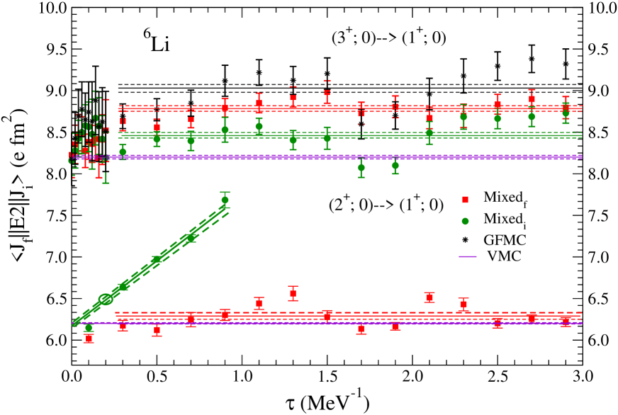
Figure 1: (Color online) $E2$ transitions for ⁶Li$(3^{+};0)$ and ⁶Li$(2^{+};0)$ to ⁶Li$(1^{+};0)$ ground state.

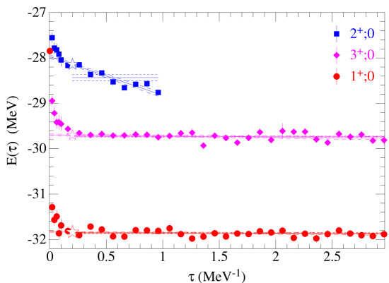
Figure 2: (Color online) GFMC E($\tau$) for different states of ⁶Li.

The $E2$ transition from $(2^{+};0)$ excited state to the ground state turns out to be difficult to calculate, as can be seen in Fig. 1. The plot shows that the GFMC mixed estimates using either the ground or the first excited $(3^{+};0)$ states of ⁶Li nucleus are moderately stable. On the other hand the GFMC mixed estimate which uses the broad $(2^{+};0)$ state of ⁶Li is growing rapidly with $\tau$, which makes a simple average meaningless. This is undoubtedly related to the difficulty in obtaining GFMC energies for broad, particle-unstable, states. Figure 2 shows the computed energies of the $(1^{+};0)$, $(3^{+};0)$, and $(2^{+};0)$ states in ⁶Li as a function of $\tau$. The $(1^{+};0)$ and $(3^{+};0)$ energies drop rapidly with $\tau$ from the initial VMC value and then become constant, aside from statistical fluctuations. The stable energy is reached around $\tau=0.2$ MeV^-1 as marked in the figure by the open stars. However, after a similar initial rapid decrease, the energy of the experimentally broad $(2^{+};0)$ state continues to decrease. At the same time the rms radius is steadily increasing; the GFMC algorithm is propagating this state to separated $\alpha$ and deuteron clusters. Based on the convergence of the $(1^{+};0)$ and $(3^{+};0)$ energies, we assume that values at $\tau=0.2$ MeV^-1 represent the best GFMC estimates for this state. Using this value of $\tau$ for the transition results in the value 6.49(16) for the $\langle 2^{+}||E2||1^{+}\rangle$ $M_{i}$ matrix element, which is shown as an open circle in Figure 1. The quoted error is based on a range of $\pm 0.1$ for the $\tau$ at which the value is evaluated. This GFMC result for the width is only 10% larger than the VMC value, but is three times as big as the CK value, and twice as big as the experimental value, which however has a sizeable error bar.

A similar analysis was used for the ⁶He $E2$ matrix element given in Table 1. The experimental value here is taken from a recent measurement of the B($E2\Uparrow$) from ⁶He breakup on ²⁰⁹Bi near the Coulomb barrier Kolata .

The GFMC propagation for the $M1$ transition ⁶Li$(0^{+};1)\to^{6}$Li$(1^{+};0)$ is shown in Fig. 3. The GFMC matrix element reduces the VMC estimate slightly, giving a width that is smaller than the current experimental value. However, this is not unexpected as we have used only one-body transition operators in our present calculation. Two-body meson-exchange currents (MEC) are known to increase isovector magnetic moments by 15-20$\%$ for $A=3$ nuclei, while having profound effects on the magnetic form factors CS98 . A previous VMC calculation of the width of this transition found a 20% increase from 7.49(2) eV to 9.06(7) eV when MEC appropriate for the AV18+UIX Hamiltonian were added WS98 . A similar increase applied to the present GFMC calculation would predict a width of 8.29(3) eV in excellent agreement with the experimental width of 8.19(17) eV. We plan to evaluate MEC corrections with the GFMC wave functions in future work. The NCSM result is in good agreement with experiment without any MEC contributions; if the MEC contributions are the size we expect, however, this good agreement will be lost when they are added.

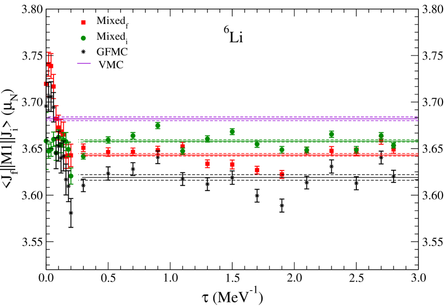
Figure 3: (Color online) $M1$ transition for ⁶Li$(0^{+};1)$ to ⁶Li$(1^{+};0)$.

Finally, we have a very difficult time evaluating the $M1$ transition between ⁶Li$(2^{+};1)$ and ⁶Li$(1^{+};0)$ states. The former is again a wide state which has the same GFMC propagation difficulty as the $E2$ transition between ⁶Li$(2^{+};0)$ and ⁶Li$(1^{+};0)$ states discussed above. However, the biggest problem is a large cancellation between different $LS[n]$ components of the two wave functions, because the dominant pieces, ¹D${}_{2}[42]$ and ³S${}_{1}[42]$, are not connected by the $M1$ operator. The VMC diagonalization and GFMC propagation are driven to minimize the energy, and may not determine small components of the wave functions sufficiently well to obtain such sensitive cancellations. Finally, the contribution of MEC terms may be much more important here because of the cancellations in the impulse approximation; hints of this were observed in the earlier VMC study WS98 .

IV.2 Electromagnetic Transitions of $A=7$ Nuclei

In Table 3 we present the matrix elements of a number of electromagnetic transitions in $A=7$ nuclei. As in Table 1, this table shows the VMC estimates, the two mixed estimates and the GFMC extrapolated matrix elements for each transition. We suppress the isospin quantum numbers for different states of ⁷Li and ⁷Be because all states we consider have $T=\frac{1}{2}$. For those transitions in $A=7$ nuclei between particle-stable states, we made two independent calculations using both Type I and Type II trial wave functions as discussed in Sec. II. However, the Type II trial function is not defined for particle-unstable states like ⁷Li($\frac{7}{2}^{-}$). It is expected that, even though the VMC estimates may be somewhat dependent on the trial wave functions, the GFMC calculation should remove most of the dependence. (It is exact at the order of $|\Psi_{0}-\Psi_{T}|^{2}$). The extrapolated regular (I) and asymptotic (II) expectation values are within $2\%$ of each other for every transition we considered.

Table 3: Electromagnetic transition reduced matrix elements of $A=7$ nuclei.

$J^{\pi}_{i}\to J^{\pi}_{f}$	$\Psi_{T}$	mode	VMC	$M_{i}$	$M_{f}$	GFMC
7Li$(\frac{1}{2}^{-})\to^{7}$Li$(\frac{3}{2}^{-})$	I	$E2(e~{}{\rm fm}^{2})$	5.11(5)	5.44(2)	5.37(2)	5.69(6)
7Li$(\frac{1}{2}^{-})\to^{7}$Li$(\frac{3}{2}^{-})$	II	$E2(e~{}{\rm fm}^{2})$	5.38(6)	5.53(3)	5.56(2)	5.71(7)
7Li$(\frac{1}{2}^{-})\to^{7}$Li$(\frac{3}{2}^{-})$	I	$M1(\mu_{N})$	2.742(1)	2.749(3)	2.693(2)	2.695(4)
7Li$(\frac{1}{2}^{-})\to^{7}$Li$(\frac{3}{2}^{-})$	II	$M1(\mu_{N})$	2.738(1)	2.673(3)	2.706(2)	2.641(3)
7Li$(\frac{7}{2}^{-})\to^{7}$Li$(\frac{3}{2}^{-})$	I	$E2(e~{}{\rm fm}^{2})$	7.67(4)	8.28(3)	8.30(3)	8.91(6)
7Be$(\frac{1}{2}^{-})\to^{7}$Be$(\frac{3}{2}^{-})$	I	$E2(e~{}{\rm fm}^{2})$	8.51(3)	9.09(4)	9.54(3)	10.12(6)
7Be$(\frac{1}{2}^{-})\to^{7}$Be$(\frac{3}{2}^{-})$	II	$E2(e~{}{\rm fm}^{2})$	8.86(13)	9.74(7)	9.60(6)	10.48(16)
7Be$(\frac{1}{2}^{-})\to^{7}$Be$(\frac{3}{2}^{-})$	I	$M1(\mu_{N})$	2.423(2)	2.412(2)	2.403(3)	2.394(4)
7Be$(\frac{1}{2}^{-})\to^{7}$Be$(\frac{3}{2}^{-})$	II	$M1(\mu_{N})$	2.405(3)	2.390(2)	2.386(5)	2.372(6)

Table 4 shows the corresponding widths of the electromagnetic transitions in $A=7$ nuclei, compared to the CK shell-model values CK65 and experiment exp567 ; li7 . The GFMC width is about 20% bigger than the CK and VMC values, and in good agreement with the experimental width for the ⁷Li$(\frac{1}{2}^{-})\to^{7}$Li$(\frac{3}{2}^{-})$ $E2$ transition. The corresponding transition in ⁷Be has not been measured. The widths for both the $M1$ transitions are relatively smaller than the corresponding experimental widths as expected for just one-body magnetic-moment operator expectation values. If there is a 20% additional contribution as expected from MEC terms, these will approach within 10% of the experimental values.

Table 4: Electromagnetic transition widths in eV of $A=7$ nuclei.

$J^{\pi}_{i}\to J^{\pi}_{f}$	$\Psi_{T}$	EM mode	CK	VMC	GFMC	Expt.
7Li$(\frac{1}{2}^{-})\to^{7}$Li$(\frac{3}{2}^{-})$	I	$E2$ ($10^{-7}$)	2.79	2.61(3)	3.24(7)	3.30(20)
7Li$(\frac{1}{2}^{-})\to^{7}$Li$(\frac{3}{2}^{-})$	II	$E2$ ($10^{-7}$)	—	2.90(3)	3.26(8)	3.30(20)
7Li$(\frac{1}{2}^{-})\to^{7}$Li$(\frac{3}{2}^{-})$	I	$M1$ ($10^{-3}$)	5.69	4.74(3)	4.58(3)	6.30(31)
7Li$(\frac{1}{2}^{-})\to^{7}$Li$(\frac{3}{2}^{-})$	II	$M1$ ($10^{-3}$)	—	4.73(1)	4.41(1)	6.30(31)
7Li$(\frac{7}{2}^{-})\to^{7}$Li$(\frac{3}{2}^{-})$	I	$E2$ ($10^{-2}$)	0.98	1.29(1)	1.74(2)	1.50(20)
7Be$(\frac{1}{2}^{-})\to^{7}$Be$(\frac{3}{2}^{-})$	I	$E2$ ($10^{-7}$)	—	4.24(3)	6.00(7)	—
7Be$(\frac{1}{2}^{-})\to^{7}$Be$(\frac{3}{2}^{-})$	II	$E2$ ($10^{-7}$)	—	4.60(13)	6.44(19)	—
7Be$(\frac{1}{2}^{-})\to^{7}$Be$(\frac{3}{2}^{-})$	I	$M1$ ($10^{-3}$)	—	2.69(1)	2.62(1)	3.43(45)
7Be$(\frac{1}{2}^{-})\to^{7}$Be$(\frac{3}{2}^{-})$	II	$M1$ ($10^{-3}$)	—	2.65(1)	2.57(1)	3.43(45)

The GFMC propagation for the $E2$ transition from ⁷Li$(\frac{7}{2}^{-})$ to ⁷Li$(\frac{3}{2}^{-})$ is illustrated in Figure 4. We note that even though the individual points for the two mixed estimates are a little scattered, the average values for these overlap. The extrapolated GFMC result is larger than the VMC estimate by 15%, making the transition width 30% larger. The VMC value is one experimental standard deviation below the experimental value li7 while the GFMC value is the same amount above the experimental value.

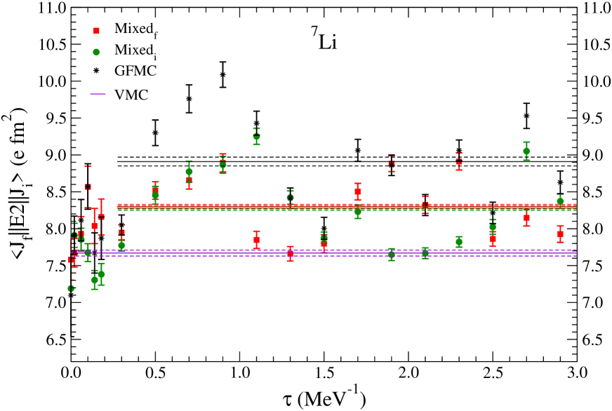
Figure 4: (Color online) $E2$ transition for ⁷Li$(\frac{7}{2}^{-})$ to ⁷Li$(\frac{3}{2}^{-})$.

IV.3 Weak Transitions in $A=6,7$ nuclei

The weak Fermi and Gamow-Teller matrix elements in $A=6,7$ nuclei are shown in Table 5. We note that in every F and GT transition the extrapolated GFMC matrix elements are smaller than the VMC estimates. However, the reduction is not large, being about $2\%$ for GT terms. This suggests the starting trial functions are already good approximations for these weak transitions. The differences between Type I and Type II trial functions are not great, and the GFMC propagation does not reduce these differences.

The Fermi matrix element for ⁷Be$(\frac{3}{2}^{-})$ to ⁷Li$(\frac{3}{2}^{-})$ is exactly 2 for charge-symmetric wave functions such as our Type I. The Type II wave functions are not charge-symmetric because the $\alpha t$ and $\alpha\tau$ separation energies in Eq.(14) are different and also the triton and ³He clusters are slightly different. It appears that the GFMC propagation will introduce only a small asymmetry when starting from a charge-symmetric (Type I) trial function, but if given a small starting asymmetry (Type II), it can enhance it considerably. However, as noted at the end of Sec. III, the present calculations may still seriously underestimate this asymmetry and its effect on $\langle||F||\rangle$. We also show in the last line of Table 5 the GT matrix element for the transition from ⁷Be($\frac{1}{2}^{-}$) to ⁷Li($\frac{3}{2}^{-}$) which is not an observable weak decay, but could be measured in a ($p,n$) reaction. The charge-symmetric Type I trial function would give the same result as the ⁷Be($\frac{3}{2}^{-}$) to ⁷Li($\frac{1}{2}^{-}$) transition, but the Type II trial function gives a very slightly different result.

Table 5: Weak transition reduced matrix elements of $A=6,7$ nuclei.

$J^{\pi}_{i}\to J^{\pi}_{f}$	$\Psi_{T}$	mode	VMC	$M_{i}$	$M_{f}$	GFMC
6He$(0^{+};1)\to^{6}$Li$(1^{+};0)$	I	GT	2.195(1)	2.176(1)	2.175(1)	2.157(1)
6He$(0^{+};1)\to^{6}$Li$(1^{+};0)$	II	GT	2.253(3)	2.184(1)	2.276(1)	2.207(3)
7Be$(\frac{3}{2}^{-})\to^{7}$Li$(\frac{3}{2}^{-})$	I	F	2.0000(0)	1.9998(1)	1.9998(1)	1.9997(3)
7Be$(\frac{3}{2}^{-})\to^{7}$Li$(\frac{3}{2}^{-})$	II	F	1.9995(1)	1.9987(3)	1.9983(3)	1.9976(5)
7Be$(\frac{3}{2}^{-})\to^{7}$Li$(\frac{3}{2}^{-})$	I	GT	2.325(1)	2.298(1)	2.301(1)	2.274(2)
7Be$(\frac{3}{2}^{-})\to^{7}$Li$(\frac{3}{2}^{-})$	II	GT	2.339(4)	2.311(1)	2.319(1)	2.291(4)
7Be$(\frac{3}{2}^{-})\to^{7}$Li$(\frac{1}{2}^{-})$	I	GT	2.146(2)	2.119(3)	2.129(3)	2.099(4)
7Be$(\frac{3}{2}^{-})\to^{7}$Li$(\frac{1}{2}^{-})$	II	GT	2.139(1)	2.121(1)	2.098(2)	2.080(1)
7Be$(\frac{1}{2}^{-})\to^{7}$Li$(\frac{3}{2}^{-})$	II	GT	2.138(1)	2.125(3)	2.104(1)	2.092(3)

The log($ft$) values obtained from VMC, shown in Table 6, are already in reasonable agreement with the corresponding experimental values and the GFMC values are even better. The previous VMC study SW02 included MEC contributions which boosted the GT transition matrix elements $\sim 1.5\%$ for $A=6$, and $\sim 3\%$ for $A=7$. This resulted in too small a half-life for ⁶He but about right for ⁷Be. When MEC contributions are eventually added to the GFMC calculation, the half-life for ⁶He should be quite good, but the rate for ⁷Be will probably be a little too fast. The last two lines of Table 6 give the branching ratio $\xi$ of the weak decay to the two final states in ⁷Li for Type I and II trial functions. These are also a little low compared to experiment, but MEC contributions should also improve the agreement.

Table 6: Log($ft$) values for weak transitions of $A=6,7$ nuclei

$J^{\pi}_{i}\to J^{\pi}_{f}$	$\Psi_{T}$	Weak Current	CK	NCSM	VMC	GFMC	Expt.
6He$(0^{+};1)\to$ 6Li$(1^{+};0)$	I	GT	2.84	2.87	2.901(1)	2.916(1)	2.910(2)
6He$(0^{+};1)\to$ 6Li$(1^{+};0)$	II	GT	—	—	2.879(2)	2.897(2)	—
7Be$(\frac{3}{2}^{-})\to^{7}$Li$(\frac{3}{2}^{-})$	I	F & GT	3.38	3.30	3.288(1)	3.302(1)	3.32
7Be$(\frac{3}{2}^{-})\to^{7}$Li$(\frac{3}{2}^{-})$	II	F & GT	—	—	3.285(1)	3.297(1)	—
7Be$(\frac{3}{2}^{-})\to^{7}$Li$(\frac{1}{2}^{-})$	I	GT	3.46	3.53	3.523(1)	3.542(1)	3.55
7Be$(\frac{3}{2}^{-})\to^{7}$Li$(\frac{1}{2}^{-})$	II	GT	—	—	3.526(1)	3.550(1)	—
$\xi$ Li$(\frac{1}{2}^{-})/$Li$(\frac{3}{2}^{-})$	I	F & GT	14.2%	10.38%	10.38(3)%	10.25(3)%	10.44(4)%
$\xi$ Li$(\frac{1}{2}^{-})/$Li$(\frac{3}{2}^{-})$	II	F & GT	—	—	10.25(3)%	10.00(3)%	—

In Fig. 5 we present the various reduced matrix elements as a function of $\tau$ for two Gamow-Teller transitions, ⁷Be$(\frac{3}{2}^{-})$ to ⁷Li$(\frac{3}{2}^{-})$ and ⁷Be$(\frac{3}{2}^{-})$ to ⁷Li$(\frac{1}{2}^{-})$. The former is shown for the Type I trial function, and the latter for the Type II. The GFMC mixed estimate points for both transitions are quite stable.

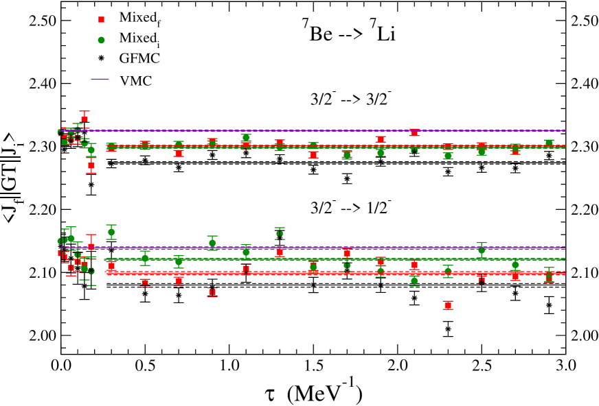
Figure 5: (Color online) Gamow-Teller transitions for ⁷Be$(\frac{3}{2}^{-})$ to ⁷Li$(\frac{3}{2}^{-})$ and ⁷Be$(\frac{3}{2}^{-})$ to ⁷Li$(\frac{1}{2}^{-})$.

V Conclusions

These first GFMC calculations of transition matrix elements in light $A=6,7$ nuclei are generally in good agreement with the current experimental data. A number of these transitions have been calculated previously using the more approximate VMC technique with an older $3N$ potential WS98 ; LW01 ; SW02 . Here we explored a significant number of electroweak transitions using the GFMC method, and calculated the corresponding widths or log($ft$) for each transition. We compared our results to Cohen-Kurath shell-model and no-core shell-model results where available, and also with the current experimental results. In most of the transitions we considered we found that the GFMC transition widths or log($ft$) values have been improved from the VMC and are in good agreement with experimental numbers. This is in general true for most of the $E2$ and all the GT and F type transitions. However, for $M1$ type transitions the GFMC widths we obtained are smaller than the current experimental values. Meson-exchange current corrections are expected to be large for $M1$ transitions and must be calculated for a meaningful comparison with data. We note here that the effect of MEC on $E2$ and GT transitions are expected to be smaller, about $\leq 3\%$. In addition to the good results we obtained in most cases we faced some difficulties, especially treating broad nuclear states using the GFMC method. In these cases scattering boundary conditions should be used; GFMC has recently been successfully applied to the $n\alpha$ scattering states NPWCH07 . We also had difficulty when the main components of the wave functions did not contribute to the transition, with the result depending on cancellations between small components.

Some of the transitions that we explored were also treated by using two different types of trial wave functions. The extrapolated GFMC values obtained by using either of the wave functions should be the same; in practice they are within 2% of each other. This is indeed found in our calculations; the widths we obtain by using one or the other type of trial wave function are very close.

In future, we expect to extend this work to larger nuclei in the $A$=8-10 range and for additional operators such as $E1$ and $M3$. One difficulty we anticipate is that some transitions of interest, such as the weak decays of ⁸He, ⁸Li, and ⁸B, run predominantly from large components of the initial state wave function to small components in the final states. These small components may not be well-determined by the GFMC calculation so additional constraints may be necessary. We also need to evaluate two-body contributions to the electroweak current operators that are consistent with our chosen Hamiltonian.

- (1) S. C. Pieper and R. B. Wiringa, Annu. Rev. Nucl. Part. Sci. 51, 53 (2001).
- (2) S. C. Pieper, K. Varga, and R. B. Wiringa, Phys. Rev. C 66, 044310 (2002).
- (3) S. C. Pieper, R. B. Wiringa, and J. Carlson, Phys. Rev. C 70, 054325 (2004).
- (4) S. C. Pieper, Nucl. Phys. A751, 516c (2005).
- (5) K. M. Nollett, S. C. Pieper, R. B. Wiringa, J. Carlson, and G. M. Hale Phys. Rev. Lett. 99, 022502 (2007).
- (6) R. B. Wiringa and R. Schiavilla, Phys. Rev. Lett. 81, 4317 (1998).
- (7) T.-S. H. Lee and R. B. Wiringa, Phys. Rev. C 63, 014006 (2000).
- (8) R. Schiavilla and R. B. Wiringa, Phys. Rev. C 65, 054302 (2002).
- (9) K. M. Nollett, R. B. Wiringa, and R. Schiavilla, Phys. Rev. C 63, 024003 (2001).
- (10) K. M. Nollett, Phys. Rev. C 63, 054002 (2001).
- (11) R. B. Wiringa, V. G. J. Stoks, and R. Schiavilla, Phys. Rev. C 51, 38 (1995).
- (12) S. C. Pieper, V. R. Pandharipande, R. B. Wiringa, and J. Carlson, Phys. Rev. C 64, 014001 (2001).
- (13) R. B. Wiringa, Phys. Rev. C 43, 1585 (1991).
- (14) B. S. Pudliner, V. R. Pandharipande, J. Carlson, S. C. Pieper, and R. B. Wiringa, Phys. Rev. C 56, 1720 (1997).
- (15) N. Metropolis, A. W. Rosenbluth, M. N. Rosenbluth, A. H. Teller, and E. Teller, J. Chem. Phys. 21, 1087 (1953).
- (16) S. Cohen and D. Kurath, Nucl. Phys. 73, 1 (1965)
- (17) A. Bohr and B. R. Mottelson, Nuclear Structure Volume I, (W. A. Benjamin, New York, 1969), Appendix 1C.
- (18) J. Carlson, Phys. Rev. C 36, 2026 (1987).
- (19) J. Carlson, Phys. Rev. C 38, 1879 (1988).
- (20) R. B. Wiringa, S. C. Pieper, J. Carlson, and V. R. Pandharipande, Phys. Rev. C 62, 014001 (2000).
- (21) M. H. Kalos, J. Comp. Phys. 2, 257 (1967).
- (22) G. P. Kamuntavičius, P. Navrátil, B. R. Barrett, G. Sapragonaite, and R. K. Kalinauskas, Phys. Rev. C 60, 044304 (1999).
- (23) R. Schiavilla, et al., Phys. Rev. C 58, 1263 (1998).
- (24) P. Navrátil and W. E. Ormand, Phys. Rev. C 68, 034305 (2003).
- (25) D. R. Tilley, C. M. Cheves, J. L. Godwin, G. M. Hale, H. M. Hofmann, J. H. Kelley, C. G. Sheu, and H. R. Weller, Nucl. Phys. A708, 3 (2002).
- (26) J. J. Kolata, et al., Phys. Rev. C 75, 031302(R) (2007).
- (27) I. Stetcu, B. R. Barrett, P. Navrátil, and J. P. Vary, Phys. Rev. C 71, 044325 (2005).
- (28) J. Carlson and R. Schiavilla, Rev. Mod. Phys. 70, 743 (1998).
- (29) Based on =17.5 fm4 by R. M. Hutcheon and H. S. Caplan, Nucl. Phys. A127, 417 (1989) and our generous error estimate.