Abstract

When all Green’s functions are known in a given gauge we may raise a question of whether it is possible or not to derive the corresponding ones in a different gauge. The answer is negative in QCD but affirmative in QED provided that we confine ourselves to the covariant gauge characterized by a gauge parameter $\alpha$. We shall discuss the physical significance of this conclusion.

1 Introduction

In quantizing a gauge-invariant Lagrangian we encounter a well-known difficulty in finding the canonical conjugate of the time-component of the gauge field. This is a reflection of the non-uniqueness of the solution of the gauge field equation due to the gauge freedom. This difficulty has been resolved in QED by Fermi’s introduction of the gauge-fixing term into the Lagrangian that provides us with the lacking canonical conjugate.

Once the theory is quantized by this method, however, the introduction of indefinite metric is indispensable since the vector field is obliged to inherit it from the Minkowski metric. This means that the state vector space resulting from the quantization of the gauge field is larger than needed for physical interpretation, and we have to pick out its physical subspace by introducing a subsidiary condition. This condition plays a dual role of eliminating the indefinite metric inherent in the state vector space as well as of recovering the classical gauge field equation, not modified by the gauge-fixing term, in the physical subspace.

In the present paper we shall confine ourselves to the so-called covariant gauge specified by a parameter $\alpha$ called the gauge parameter. Quantized gauge theories are no longer invariant under local gauge transformations because of the presence of the gauge-fixing term, but it so happens that the resulting theory is invariant under new global transformations called the BRS transformations [1].

In Section 2 we shall reinstate the essence of the BRS transformations in connection wit the gauge-dependence of Green’s functions and shall clarify the condition under which Green’s functions become gauge-independent. In tackling the problem of gauge-dependence the renormalization group (RG) approach [2, 3] is useful and it is briefly recapitulated in Section 3 with an emphasis on the gauge field propagator.

The question of gauge-dependence was once raised by Shirkov in connection with the use of RG in perturbative QCD [4]. The results depend sensitively on the renormalization scheme so that we propose here a scheme of making the beta-function independent of the gauge parameter $\alpha$.

In Section 4 the RG equations for the running coupling constant and gauge parameter are solved and their ultra-violet asymptotic limits are studied to answer the question of gauge-dependence of Green’s functions. For this purpose we derive a sum rule [5, 6] which enables us to express the renormalization constant $Z_{3}^{-1}$ in a simple form.

Green’s functions defined as the vacuum expectation values of the time-ordered products of BRS invariant operators are always independent of $\alpha$, but those made up of BRS variant ones are $\alpha$-dependent. For the latter an important question is whether it is possible or not to continue Green’s functions analytically as functions of $\alpha$. When it is possible to continue them from $\alpha_{1}$ to $\alpha_{2}$, we say that $\alpha_{1}$ and $\alpha_{2}$ are connected. Then, mutually connected values of $\alpha$ form a set called an equivalence class of gauges, and we may ask how many equivalence classes of gauges there are in QCD and also in QED. The answer is that three in QCD and one in QED, respectively. QED is simple, but QCD is complicated and we may ask what the multiplicity of equivalence classes would mean. We shall discuss the physical significance of these results in connection with the gluon mass.

In Section 5 this quest is further pursued by extending the gauge parameter $\alpha$ into the complex plane.

2 BRS Invariance

Local gauge transformations in classical gauge theory are replaced by global BRS transformations and we shall briefly recapitulate their properties

BRS transformations

The standard Lagrangian density of a gauge theory, say QCD, is given by

$${\cal L}={\cal L}_{{inv}}+{\cal L}_{{gf}}+{\cal L}_{{FP}}$$ (2.1)

where ${\cal L}_{{inv}}$ denotes the classical gauge-invariant part, ${\cal L}_{{gf}}$ the gauge-fixing terms and ${\cal L}_{{FP}}$ the Faddeev-Popov (FP) ghost term characteristic of non-Abelian gauge theories:

$${\cal L}_{{inv}} = -\frac{1}{4}F_{\mu\nu}\cdot F_{\mu\nu}-\bar{\psi}(\gamma_{\mu}D_{\mu}+m)\psi\,,$$ (2.2)

$${\cal L}_{{gf}} = \partial_{\mu}B\cdot A_{\mu}+\frac{1}{2}\alpha B\cdot B\,,$$ (2.3)

$${\cal L}_{{FP}} = i\partial_{\mu}\bar{c}\cdot D_{\mu}c\,.$$ (2.4)

in the customary notation. The gauge parameter is denoted by $\alpha$ and $D_{\mu}$ represents the covariant derivative whose explicit forms are given by

$$D_{\mu}\ \psi = (\partial_{\mu}-igT\cdot A_{\mu})\psi\,,$$ (2.5)

$$D_{\mu}\ c = \partial_{\mu}c+gA_{\mu}\times c\,.$$ (2.6)

The BRS transformations of the gauge field $A_{\mu}$ and the quark field $\psi$ are defined by replacing the infinitesimal gauge function by the FP ghost field $c$ or $\bar{c}$ in their respective infinitesimal gauge transformations:

$$\delta A_{\mu} = D_{\mu}c\,,\ \ \ \delta\psi=ig(c\cdot T)\psi\,,$$ (2.7)

$$\bar{\delta}A_{\mu} = D_{\mu}\bar{c}\,,\ \ \ \bar{\delta}\psi=ig(\bar{c}\cdot T)\psi\,.$$ (2.8)

For the auxiliary fields $B$, $c$ and $\bar{c}$ we require

$$\delta{\cal L}=\bar{\delta}{\cal L}=0\,,$$ (2.9)

then we find

$$\delta\,B=0\,,\ \ \ \delta\,\bar{c}=iB\,,\ \ \ \delta\,c=-\frac{1}{2}g\,(c\times c)\,,$$ (2.10)

$$\bar{\delta}\,\bar{B}=0\,,\ \ \ \bar{\delta}\,c=i\bar{B}\,,\ \ \ \bar{\delta}\,\bar{c}=-\frac{1}{2}g\,(\bar{c}\times\bar{c})\,,$$ (2.11)

where $\bar{B}$ is defined by

$$B+\bar{B}-ig(c\times\bar{c})=0\,.$$ (2.12)

In general the BRS transforms of a field $\phi$ are given in terms of the BRS charges $Q_{B}$ and $\bar{Q}_{B}$ by

$$\delta\,\phi=i[Q_{B},\phi]_{\mp},\ \ \ \bar{\delta}\,\phi=i[\bar{Q}_{B},\phi]_{\mp}\,,$$ (2.13)

$$Q_{B}^{2}={\bar{Q}}_{B}^{2}=Q_{B}\bar{Q}_{B}+\bar{Q}_{B}Q_{B}=0\,.$$ (2.14)

We choose the $-(+)$ sign in (2.14) when $\phi$ is even (odd) in the ghost fields $c$ and $\bar{c}$ that are anticommuting hermitian scalar fields.

The sum of the gauge-fixing and the FP ghost terms can be expressed as

$${\cal L}_{{gf}}+{\cal L}_{{FP}}=\delta(-i\partial_{\mu}\bar{c}\cdot A_{\mu}-\frac{i}{2}\alpha\,\bar{c}\cdot B)$$ (2.15)

and evidently we have

$$\delta{\cal L}_{inv}=0\,.$$ (2.16)

Namely, ${\cal L}_{inv}$ is closed and ${\cal L}_{{gf}}+{\cal L}_{{FP}}$ is exact, and

$$\delta{\cal L}=0\,.$$ (2.17)

BRS Cohomology [5]

The quantization of the gauge field and the introduction of the auxiliary fields $B$, $c$ and $\bar{c}$ introduce indefinite metric into the state vector space ${\cal V}$.

A physical state $|f\rangle$ is defined by the following subsidiary condition:

$$Q_{B}\,|f\rangle=0\,,\ \ \ \ |f\rangle\in{\cal V}\,.$$ (2.18)

In particular, the vacuum state $|0\rangle$ is physical,

$$Q_{B}\,|0\rangle=0\,.$$ (2.19)

The physical subspace ${\cal V}_{phys}$ is then defined by

$${\cal V}_{phys}=\{|f\rangle|\ \ Q_{B}|f\rangle=0\,,\ \ |f\rangle\in{\cal V}\}\,.$$ (2.20)

It is essentially a collection of closed states with respect to the nilpotent operator $Q_{B}$. We also introduce a subspace ${\cal V}_{d}$ defined by

$${\cal V}_{d}=\{Q_{B}|f\rangle|\ \ |f\rangle\in{\cal V}\}\,.$$ (2.21)

This is a collection of exact states with respect to $Q_{B}$ and the Hilbert space $\cal H$ is defined as the BRS cohomology by

$${\cal H}={\cal V}_{phys}/{\cal V}_{d}\,.$$ (2.22)

Then let us consider a set of closed operators $A,\ B,\cdots$ satisfying

$$\delta A=\delta B=\cdots=0\,,$$ (2.23)

then

$$\langle 0|\delta M\cdot AB\cdots|0\rangle=\langle 0|\delta(MAB\cdots|0\rangle=0\,,$$ (2.24)

since the vacuum state is physical.

Let ${\cal L}_{I}$ and ${\cal L}_{II}$ be two BRS invariant Lagrangian densities, namely,

$$\delta{\cal L}_{I}=\delta{\cal L}_{II}=0\,.$$ (2.25)

Furthermore, let us assume that their difference be exact:

$$\Delta{\cal L}=\delta{\cal L}_{II}-\delta{\cal L}_{I}=\delta M\,.$$ (2.26)

For instance, Lagrangian densities corresponding to two distinct values of $\alpha$ in (2.4) satisfy these two conditions since we find

$$M=-\frac{1}{2}i\,\Delta\alpha\,(\bar{c}\cdot B)\,.$$ (2.27)

Then we introduce time-ordered Green’s functions in two gauges given above.

In the gauge I we have the following path integrals:

$$\langle AB\cdots\rangle_{I}=\frac{1}{N_{I}}\int{\cal D}(path)\,AB\cdots\exp(iS_{I})$$ (2.28)

$$N_{I}=\int{\cal D}(path)\,\exp(iS_{I})\,.$$ (2.29)

${\cal D}(path)$ denotes the path integral over all the field variables, and we have similar expressions in the gauge II, and the difference between the two actions is given by

$$\Delta S=S_{II}-S_{I}=\int d^{4}x\,\Delta{\cal L}=\int d^{4}x\,\delta M\,.$$ (2.30)

Green’s functions in the gauge II can be expressed as

$$\langle AB\cdots\rangle_{II}=\frac{\langle AB\cdots\exp(i\,\Delta S)\rangle_{I}}{\langle\exp(i\,\Delta S)\rangle_{I}}\,.$$ (2.31)

Now we expand the denominator on the r.h.s. of (2.31) in powers of $\Delta S$ and use (2.26) and (2.24) to obtain

$$\langle\exp(i\,\Delta S)\rangle_{I}=1\,.$$ (2.32)

Thus (2.31) reduces to

$$\langle AB\cdots\rangle_{II}={\langle AB\cdots\exp(i\,\Delta S)\rangle_{I}}\,.$$ (2.33)

The r.h.s. can be expanded in powers of $\Delta\alpha=\alpha_{II}-\alpha_{I}$. When this expansion converges this is an analytic continuation of Green’s functions as functions of $\alpha$. When this is the case we may say that the two values of $\alpha$, $\alpha_{1}$ and $\alpha_{2}$, are connected and the set of $\alpha$ mutually connected will be called an equivalence class of gauges. The question of how many classes there are in a given gauge theory will be discussed in a later section.

When all the operators are closed, satisfying (2.23), we obtain, with the help of (2.24) the equality

$$\langle AB\cdots\rangle_{II}={\langle AB\cdots\rangle_{I}}\,.$$ (2.34)

This shows that Green’s functions cosntructed in terms of closed operators alone are gauge-independent. The $S$-matrix elements for observable hadronic processes are obtained by applying the LSZ reduction formula [7] to Green’s functions defined in terms of BRS invariant operators so that they are independent of the choice of the gauge parameter $\alpha$. Of course, this statement does not apply to Green’s functions constructed in terms of BRS variant operators, such as the gauge field propagator which we shall investigate in a later section.

3 Renormalization Group

Once Shirkov emphasized the gauge.dependence of the RG treatment in perturbative QCD [4] since the results are sensitive to the renormalization scheme. He even presented an example in which asymptotic freedom is valid only for positive values of $\alpha$ but not for negative ones. This is apparently due to the $\alpha$ dependence of the beta-function. Therefore, we shall first briefly review a renormalization scheme which makes the beta-function independent of the gauge parameter [6].

First we shall refer to (2.33) which has been derived in the unrenormalized version. The field operators $A_{\lambda}$ and $B$ and the gauge parameter $\alpha$ are multiplicatively renormalized:

$$A_{\lambda}^{(0)}=Z_{3}^{1/2}(\alpha)\,A_{\lambda}\,,\ \ \ B^{(0)}=Z_{3}^{-1/2}(\alpha)\,B\,,\ \ \ \alpha^{(0)}=Z_{3}(\alpha)\,\alpha\,,$$ (3.1)

where the superscript $(0)$ is attached to the unrenormalized expressions.

As a special case of (2.33) we shall choose $\alpha_{II}=\alpha$ and $\alpha_{I}=0$, then we have

$$\langle AB\cdots\rangle_{\alpha}=\left\langle AB\cdots\exp\left(\frac{i\alpha}{2}\int d^{4}x\,B(x)\cdot B(x)\right)\right\rangle_{0}\,,$$ (3.2)

in the unrenormalized version. The renormalized version of (3.2) takes exactly the same form because of the identity

$$\alpha^{(0)}B^{(0)}\cdot B^{(0)}=\alpha\,B\cdot B\,.$$ (3.3)

Then we introduce RG equations in the Landau gauge, $\alpha=0$. For the renormalized version of Green’s functions we have an equation of the following form:

$$({\cal D}_{0}+\gamma_{G})\langle AB\cdots\rangle_{0}=0\,,$$ (3.4)

where $\gamma_{G}$ is the anomalous dimension of Green’s function $\langle AB\cdots\rangle_{0}$ in the Landau gauge and

$${\cal D}_{0}=\mu\frac{\partial}{\partial\mu}+\beta(g)\frac{\partial}{\partial g}\,.$$ (3.5)

The anomalous dimension of the gauge field in the Landau gauge, which is obviously $\alpha$-independent, is denoted by $\gamma_{V}$.

Then the l.h.s. of (3.2), renormalized in the Landau gauge, satisfies

$$({\cal D}_{0}+\gamma_{G})\langle AB\cdots\rangle_{\alpha}=2\gamma_{V}\left\langle AB\cdots\exp\left(\frac{i\alpha}{2}\int d^{4}x\,B(x)\cdot B(x)\right)\right\rangle_{\alpha}\,.$$ (3.6)

On the other hand, we also have

$$\alpha\frac{\partial}{\partial\alpha}\langle AB\cdots\rangle_{\alpha}=\left\langle AB\cdots\exp\left(\frac{i\alpha}{2}\int d^{4}x\,B(x)\cdot B(x)\right)\right\rangle_{\alpha}\,.$$ (3.7)

Combining these two equations we find

$$({\cal D}+\gamma_{G})\langle AB\cdots\rangle_{\alpha}=0\,,$$ (3.8)

where

$${\cal D}={\cal D}_{0}+2\alpha\gamma_{V}\frac{\partial}{\partial\alpha}\,.$$ (3.9)

Next we introduce the gauge field propagator

$$\langle A^{a}_{\lambda}(x),A^{b}_{\mu}(y)\rangle=\frac{-i}{(2\pi)^{4}}\delta_{ab}\int d^{4}k\,e^{ik(x-y)}D_{\lambda\mu}(k)\,,$$ (3.10)

which is the vacuum expectation value of the time-ordered product of two color gauge field operators, and

$$D_{\lambda\mu}(k) = \left(\delta_{\lambda\mu}-\frac{k_{\lambda}k_{\mu}}{k^{2}-i\epsilon}\right)D(k^{2},\alpha)+\alpha\frac{k_{\lambda}k_{\mu}}{(k^{2}-i\epsilon)^{2}}\,,$$ (3.11)

$$D(k^{2},\alpha) = \int dm^{2}\frac{\rho(m^{2})}{k^{2}+m^{2}-i\epsilon}\,.$$ (3.12)

Then introduce

$$R(k^{2},\alpha)=k^{2}\,D(k^{2},\alpha)\,.$$ (3.13)

Since the gauge field has been renormalized in the Landau gauge, we have

$$R(\mu^{2},0)=1.$$ (3.14)

In other gauges we have to employ the renormalization factor $Z_{3}(\alpha)$ instead of $Z_{3}(0)$, and this amounts to a further renormalization for $R$. The properly renormalized $R$ function and the gauge parameter are denoted by $\bar{R}$ and $\bar{\alpha}$, respectively, and are given, in a consistent manner with (3.1), by

$$R(k^{2},\alpha) = R(\mu^{2},\alpha)\bar{R}(k^{2},\bar{\alpha})\,,$$ (3.15)

$$\alpha = R(\mu^{2},\alpha)\bar{\alpha}\,.$$ (3.16)

The function $R(k^{2},\alpha)$ renormalized in the Landau gauge satisfies

$$({\cal D}+2\gamma_{V})R(k^{2},\alpha)=0\,.$$ (3.17)

Then the function $\bar{R}(k^{2},\bar{\alpha})$ normalized by

$$\bar{R}(\mu^{2},\bar{\alpha})=1$$ (3.18)

satisfies

$$({\cal D}+2\bar{\gamma}_{V})\bar{R}(k^{2},\bar{\alpha})=0\,,$$ (3.19)

where the new anomalous dimension $\bar{\gamma}_{V}$ is given by

$$\bar{\gamma}_{V}=\gamma_{V}+\frac{1}{2}{\cal D}\ln R(\mu^{2},\alpha)\,.$$ (3.20)

Next we switch the set of parameters from $(\mu,g,\alpha)$ to $(\mu,g,\bar{\alpha})$. The anomalous dimension $\bar{\gamma}_{V}$ will be expressed as a function of $g$ and $\bar{\alpha}$, and it will be denoted by $\bar{\gamma}_{V}(g,\bar{\alpha})$ from now on. Then,

$${\cal D} = ({\cal D}\mu)\frac{\partial}{\partial\mu}+({\cal D}g)\frac{\partial}{\partial g}+({\cal D}\bar{\alpha})\frac{\partial}{\partial\bar{\alpha}}$$ (3.21)

$$= \mu\frac{\partial}{\partial\mu}+\beta(g)\frac{\partial}{\partial g}-2\bar{\alpha}\,\bar{\gamma}_{V}(g,\bar{\alpha})\frac{\partial}{\partial\bar{\alpha}}\,.$$ (3.22)

In this way we have established a renormalization prescription leading to an $\alpha$-independent beta-function. For the quark field we can derive its anomalous dimension $\bar{\gamma}_{\psi}$ in a manner similar to the above derivation of $\bar{\gamma}_{V}$. Since the beta-function is independent of $\alpha$, the concept of asymptotic freedom is gauge-independent. From now on we shall skip the bars introduced above.

4 Asymptotic Limits of Running Parameters

The RG equations for QCD have been studied in detail and we shall reinstate their essence in what follows [5, 6].

Renormalization Constants

An element of RG may be expressed as

$$R(\rho)=\exp(\rho{\cal D})\,,$$ (4.1)

where $\rho$ denotes the parameter of RG and the composition law of this group is given by

$$R(\rho)R(\rho^{\prime})=R(\rho+\rho^{\prime})\,.$$ (4.2)

Let $Q$ be a function of $g,\ \alpha$ and $\mu$, and we define the running $Q$ to be

$$\bar{Q}(\rho)=\exp(\rho{\cal D})Q(g,\alpha,\mu)=Q(\bar{g}(\rho),\bar{\alpha}(\rho),\bar{\mu}(\rho))\,,$$ (4.3)

with the initial condition

$$\bar{Q}(0)=Q\,.$$ (4.4)

Let the anomalous dimension of Green’s function $G(p_{i};g,\alpha,\mu)$ be $\gamma(g,\alpha)$, then we have

$$[{\cal D}+\gamma(g,\alpha)]G(p_{i};g,\alpha,\mu)=0\,.$$ (4.5)

Its running version is defined by

$$\bar{G}(\rho)=\exp(\rho{\cal D})\cdot G(p_{i};g,\alpha,\mu)\,,$$ (4.6)

and it satisfies

$$\frac{\partial}{\partial\rho}\bar{G}(\rho)=-\bar{\gamma}(\rho)\bar{G}(\rho)\,.$$ (4.7)

The formal solution is given by

$$G(p_{i};g,\alpha,\mu)=\exp\left[\int_{0}^{\rho}d\rho^{\prime}\bar{\gamma}(\rho^{\prime})\right]\cdot G(p_{i};\bar{g}(\rho),\bar{\alpha}(\rho),\bar{\mu}(\rho))\,.$$ (4.8)

Then we assume, in the presence of a cut-off $\Lambda$, that the running coupling constant $\bar{g}(\rho)$ tends to the unrenormalized or the bare one $g_{0}$ in the limit $\rho\to\infty$, namely,

$$\lim_{\rho\to\infty}\bar{g}(\rho)=g^{(0)}\,,$$ (4.9)

and similarly

$$\lim_{\rho\to\infty}\bar{\alpha}(\rho) = \alpha^{(0)}\,,$$ (4.10)

$$\lim_{\rho\to\infty}\bar{\mu}(\rho) = \mu\lim_{\rho\to\infty}e^{\rho}=\infty\,.$$ (4.11)

In this limit (4.8) reduces to

$$G(p_{i};g,\alpha,\mu)=\exp\left[\int_{0}^{\infty}d\rho^{\prime}\bar{\gamma}(\rho^{\prime})\right]\cdot G^{(0)}(p_{i};g^{(0)},\alpha^{(0)},\infty)\,,$$ (4.12)

where $G^{(0)}$ denotes the unrenormalized version of Green’s function $G$. Then the renormalization constant of $G$ denoted by $Z$ is given by

$$Z=\exp\left[-\int_{0}^{\infty}d\rho^{\prime}\bar{\gamma}(\rho^{\prime})\right]\,.$$ (4.13)

The solution of (3.19) reads as

$$R(k^{2};g,\alpha,\mu)=\exp\left[2\int_{0}^{\rho}d\rho^{\prime}\bar{\gamma}_{V}(\rho^{\prime})\right]\cdot R(k^{2};\bar{g}(\rho),\bar{\alpha}(\rho),\bar{\mu}(\rho))\,.$$ (4.14)

Now apply the Lehmann representation (3.12) to the l.h.s. and take the limit $\rho\to\infty$ after putting $k^{2}=\bar{\mu}^{2}(\rho)$, then with the help of (4.13) we obtain

$$Z_{3}^{-1}=\int dm^{2}\rho(m^{2})=\exp\left[2\int_{0}^{\infty}d\rho^{\prime}\bar{\gamma}_{V}(\rho^{\prime})\right]\,.$$ (4.15)

In the cut-off theory we first take the limit $\rho\to\infty$ and then $\Lambda\to\infty$, but in what follows we invert the order of limiting procedures by taking the limit $\Lambda\to\infty$ first. Thus some of the initial conditions introduced in the cut-off theory are not necessarily satisfied. As an example we shall see later that the limiting values (4.9) and (4.10) cannot be arbitrary despite our expectation that the unrenormalized $g^{(0)}$ and $\alpha^{(0)}$ should be chosen arbitrarily.

Asymptotic Limits of Running Parameters

Next we shall study the RG equations for the running parameters $\bar{g}(\rho),\ \bar{\alpha}(\rho)$ and $\bar{\mu}(\rho)$ that follow from (4.3),

$$\frac{d}{d\rho}\bar{g}(\rho) = \bar{\beta}(\rho)\,,$$ (4.16)

$$\frac{d}{d\rho}\bar{\alpha}(\rho) = -2\bar{\alpha}(\rho)\bar{\gamma}_{V}(\rho)\,,$$ (4.17)

$$\frac{d}{d\rho}\bar{\mu}(\rho) = \bar{\mu}(\rho)\ \ \mbox{or}\ \ \bar{\mu}(\rho)=\mu\,e^{\rho}\,.$$

First we shall define their asymptotic limits by

$$\bar{g}(\infty)=g_{\infty},\ \ \bar{\alpha}(\infty)=\alpha_{\infty},\ \ \bar{\mu}(\infty)=\infty\,.$$ (4.18)

In the absence of a cut-off they do not necessarily reduce to their unrenormalized counterparts in (4.9) and (4.10).

In perturbation theory $\beta(g)$ and $\gamma_{V}(g,\alpha)$ are given in the form of power series,

$$\beta(g) = g^{3}(\beta_{0}+\beta_{1}\,g^{2}+\cdots)\,,$$ (4.19)

$$\gamma_{V}(g,\alpha) = g^{2}(\gamma_{0}(\alpha)+\gamma_{1}(\alpha)\,g^{2}+\cdots)\,,$$ (4.20)

where

$$\gamma_{0}(\alpha) = \gamma_{00}+\gamma_{01}\alpha\,,$$ (4.21)

$$\gamma_{1}(\alpha) = \gamma_{10}+\gamma_{11}\alpha+\gamma_{12}\alpha^{2}\,,\ \ \cdots\,,$$ (4.22)

The lowest order coefficients are given by

$$\beta_{0} = -\frac{1}{32\pi^{2}}\left(22-\frac{4}{3}N_{f}\right)\,,$$ (4.23)

$$\gamma_{00} = -\frac{1}{32\pi^{2}}\left(13-\frac{4}{3}N_{f}\right)\,,$$ (4.24)

$$\gamma_{01} = \frac{3}{32\pi^{2}}>0\,.$$

When $\beta_{0}$ is negative, namely, when $N_{f}\leq 16$, asymptotic freedom is realized and we shall assume it in what follows.

Asymptotic freedom [8, 9] is characterized by

$$g_{\infty}=0\,,$$ (4.25)

and for large values of $\rho$ we obtain approximately

$$\bar{g}^{2}(\rho)=\frac{1}{b\rho}\ \ \ (b=-2\beta_{0}>0)\,.$$ (4.26)

By integrating the second equation in (4.16) we find a sum rule [5, 6]:

$$\ln\frac{\alpha_{\infty}}{\alpha}=-2\int_{0}^{\infty}d\rho\bar{\gamma}_{V}(\rho)\,,$$ (4.27)

or

$$Z_{3}^{-1}=\exp\left[2\int_{0}^{\infty}d\rho\bar{\gamma}_{V}(\rho)\right]=\frac{\alpha}{\alpha_{\infty}}\,.$$ (4.28)

The essence of our argument is based on this sum rule.

Our main problem is the determination of the asymptotic limit $\alpha_{\infty}$, but this problem has been discussed in detail before, so we shall only quote the results in what follows. We shall come back to it, however, in the next section for a different purpose.

For $\alpha=0$ we have $\bar{\alpha}(\rho)=0$ and hence $\alpha_{\infty}=0$. It is clear that $\bar{\alpha}(\rho)$ and $\alpha$ are always of the same signature. We find three possibilities for $\alpha_{\infty}$:

$$\alpha_{\infty}=-\infty,\ 0,\ \alpha_{0}\,,$$ (4.29)

where $\alpha_{0}$ is defined by

$$\gamma_{0}(\alpha_{0})=\gamma_{00}+\gamma_{01}\alpha_{0}=0\ \ \mbox{or}\ \ \ \alpha_{0}=-\gamma_{00}/\gamma_{01}\,.$$ (4.30)

For $\alpha_{0}>0$ or $N_{f}<10$, we find

$$\alpha_{\infty}=\left\{\begin{tabular}[]{ll}$\alpha_{0}\,,$&$\alpha>0$\\ 0\,,&$\alpha=0$\\ $-\infty\,,$&$\alpha<0\,,$\\ \end{tabular}\right.$$ (4.31)

and in this case the sum rule can be expressed as

$$\int dm^{2}\,\rho(m^{2})=\frac{\alpha}{\alpha_{\infty}}\theta(\alpha)$$ (4.32)

where

$$\theta(\alpha)=\left\{\begin{tabular}[]{ll}$1\,,$&$\alpha\geq 0$\\ 0\,,&$\alpha<0$\,.\\ \end{tabular}\right.$$ (4.33)

The r.h.s. of (4.32) is a continuous function of $\alpha$, but its derivative with respect to $\alpha$ develops a discontinuity at $\alpha=0$. Thus, the set of real $\alpha$, denoted by $D$, is divided into three connected subsets:

$$D=D(-\infty)\bigcup D(0)\bigcup D(\alpha_{0})\,,$$ (4.34)

where we confine ourselves to positive $\alpha_{0}$ or $N_{f}<10$

$$D=\{\alpha|\ \ \alpha\in{R}\}\,,$$ (4.35)

$$D(-\infty)=\{\alpha|\ \ \alpha<0\}\,,$$ (4.36)

$$D(0)=\{\alpha|\ \ \alpha=0\}\,,$$ (4.37)

$$D(\alpha_{0})=\{\alpha|\ \ \alpha>0\}\,.$$ (4.38)

Thus, for gauge-dependent Green’s functions such as the gluon propagator we find three equivalence classes of gauges.

In one of the papers by the present authors [10] the residue of the massless pole in the two-point function

$$\langle A_{\lambda}^{a}(x),F_{\mu\nu}^{b}(y)\rangle$$ (4.39)

has been studied, and it has been concluded that the residue vanishes in two classes $D(-\infty)$ and $D(0)$, suggesting that the gluon in these gauges would likely be massive, whereas it is non-vanishing in the class $D(\alpha_{0})$ implying zero mass for the gluon. This means that the gluon mass would be gauge-dependent. The interpretation of this result is delicate. In that paper we tacitly assumed that the gluon mass is a physical quantity and that the above result indicates the gauge-dependence of QCD, or more precisely the class-dependence of the gluon mass, namely, it is zero in the equivalence class of gauges $D(\alpha_{0})$, but it is non-zero in the classes $D(-\infty)\bigcup D(0)$. The gluon mass denoted by $M$ must be RG invariant

$${\cal D}M=0$$ (4.40)

within a class.

We found that this interpretation is misleading since the physically observable quantities must be gauge-independent as illustrated by (2.34).

The $S$-matrix elements for hadronic processes are gauge-independent as is clear from (2.34), and the condition for color confinement [5, 6, 11, 12, 13]

$$Z_{3}^{-1}=0$$ (4.41)

is satisfied in the classes $D(-\infty)\bigcup D(0)$. Therefore, in these classes color confinement is realized and the unitarity condition of the $S$-matrix between two hadronic states $|a\rangle$ and $|b\rangle$ reads as

$$\sum_{n}\langle b|S^{\dagger}|n\rangle\langle n|S|a\rangle=\langle b|a\rangle\,,$$ (4.42)

where the sum over the intermediate states is saturated by hadronic states alone without introduction of the confined quarks and gluons. Since the $S$-matrix is gauge-independent this statement is also valid for the class $D(\alpha_{0})$. Thus, confinement is a gauge-independent or class-independent concept. This conclusion does not contradict the gauge-dependence of the gluon mass since the mass of the confined gluons is never observed and turns out to be an unphysical quantity. A similar observation has been made by Fujikawa, Lee and Sanda [14], that particles with gauge-dependent masses are unphysical and not subject to observation in connection with the $R_{\xi}$ gauge.

5 Introduction of the Complex Gauge Parameter

From (4.20) and (4.22) we can readily deduce that $\gamma_{V}$ can be expanded into a double power series in $g^{2}$ and $\alpha g^{2}$. For sufficiently large $\rho$, we can assume that $\bar{g}^{2}(\rho)\ll 1$ and if $\bar{\alpha}(\rho)$ is bounded below a certain constant, we may use perturbation theory in powers of $g^{2}$. In the lowest order we have

$$\frac{d\bar{g}}{d\rho}=\beta(\bar{g})\approx\beta_{0}\bar{g}^{3}=-\frac{b}{2}\bar{g}^{3}\,,$$ (5.1)

and its solution is given by

$$\bar{g}^{2}(\rho)=\frac{g^{2}}{1+b\,g^{2}\,\rho}\,.$$ (5.2)

When $\bar{\alpha}$ is bounded we employ the following approximate equation:

$$\frac{d\bar{\alpha}}{d\rho}=-2\bar{\alpha}\bar{\gamma}_{V}\approx f(\rho)\bar{\alpha}(\alpha_{0}-\bar{\alpha})\,,$$ (5.3)

where

$$f(\rho)=2\,\gamma_{01}\,\bar{g}^{2}(\rho)>0\,.$$ (5.4)

When the integral (4.27) is convergent, $\alpha_{\infty}$ must be finite. The expansion of $\gamma_{V}$ in powers of $g^{2}$ starts from $g^{2}$ and for large values of $\rho$ the behavior of $\bar{g}^{2}(\rho)$ is given by (4.26) so that the integral of the first term in the expansion of $\bar{\gamma}_{V}$ diverges like

$$\int_{0}^{\infty}d\rho\,\bar{g}^{2}(\rho)\sim\frac{1}{b}\ln\infty\,.$$ (5.5)

In order for the integral of the power series to converge term by term in (4.27), therefore, the condition

$$\gamma_{0}(\alpha_{\infty})=0$$ (5.6)

must be satisfied. With reference to (4.30) we find

$$\alpha_{\infty}=\alpha_{0}$$ (5.7)

When the integral (4.27) is divergent, $\ln(\alpha/\alpha_{\infty})$ should diverge so that we find

$$\alpha_{\infty}=0\ \ \mbox{or}\ \ \pm\infty\,.$$ (5.8)

Now, when $\bar{\alpha}$ goes off $\alpha_{\infty}$ starting from its neighborhood for increasing $\rho$, $\alpha_{\infty}$ is called a repulsive asymptotic limit. Otherwise, when $\bar{\alpha}$ approaches $\alpha_{\infty}$ again starting from its neighborhood, it is called an attractive asymptotic limit.

Case of positive $\alpha_{0}$ ($N_{f}<10$)

Integration of (5.3) in the neighborhood of $\alpha_{0}$ yields

$$\frac{\alpha_{0}-\bar{\alpha}(\rho)}{\alpha_{0}-\alpha}\cong\exp\left[-\alpha_{0}\int_{0}^{\rho}d\rho^{\prime}\,f(\rho^{\prime})\right]\to 0\,,\ \ \ \mbox{for}\ \ \ \rho\to\infty\,.$$ (5.9)

Thus $\alpha_{0}$ is found to be attractive. In the neighborhood of 0, on the other hand, we find

$$\frac{\bar{\alpha}(\rho)}{\alpha}\cong\exp\left[\alpha_{0}\int_{0}^{\rho}d\rho^{\prime}\,f(\rho^{\prime})\right]\to\infty\,,\ \ \ \mbox{for}\ \ \ \rho\to\infty\,.$$ (5.10)

Thus $\alpha_{\infty}=0$ is found to be repulsive.

The flow of $\alpha(\rho)$ on the real $\alpha$ axis for increasing $\rho$ is given in Fig. 1.

Figure 1: Flow of $\bar{\alpha}(\rho)$ along the real $\alpha$ axis for increasing $\rho$ ($\alpha_{0}>0$).

From Fig. 1 we conclude that $-\infty$ is also attractive.

Case of negative $\alpha_{0}$ ($10\leq N_{f}\leq 16$)

In this case 0 and $-\infty$ are attractive and $\alpha_{0}$ is repulsive.

Figure 2: Flow of $\bar{\alpha}(\rho)$ along the real $\alpha$ axis for increasing $\rho$ ($\alpha_{0}<0$).

In what follows we shall confine ourselves to the case of positive $\alpha_{0}$ and shall study what would take place when $\alpha$ turns out to be complex while keeping $g^{2}$ real. For this purpose we assume that $g^{2}$ is already sufficiently small and that $|\bar{\alpha}(\rho)|$ is bounded to guarantee the following treatment of the RG equations.

The solution of (5.3) as combined with (5.2) is given by

$$\bar{\alpha}(\rho)=\alpha_{0}\left[\left(\frac{\alpha_{0}}{\alpha}-1\right)(1+b\,g^{2}\,\rho)^{-n}+1\right]^{-1}\,,$$ (5.11)

where

$$n=\gamma_{00}/\beta=\left(13-\frac{4}{3}N_{f}\right)/\left(22-\frac{4}{3}N_{f}\right)\,.$$ (5.12)

For $\alpha_{0}>0$ we have $n>0$.

(1) $\alpha>0$

In this case we can easily check for $\rho>0$ that

$$\left(\frac{\alpha_{0}}{\alpha}-1\right)(1+b\,g^{2}\,\rho)^{-n}+1>0\,,$$ (5.13)

and, as has been expected, we have

$$\lim_{\rho\to\infty}\bar{\alpha}(\rho)=\alpha_{0}\,.$$ (5.14)

(2) $\alpha=0$

In this case, $\alpha=0$ is a fixed point, so that we have $\bar{\alpha}(\rho)=0$, and consequently

$$\lim_{\rho\to\infty}\bar{\alpha}(\rho)=0\,.$$ (5.15)

(3) $\alpha<0$

The asymptotic limit of $\bar{\alpha}(\rho)$, when we start from a negative $\alpha$, should be equal to either 0 or $-\infty$. Since $\alpha_{\infty}=0$ is repulsive, $\alpha_{\infty}=-\infty$ is the only choice. In this case we cannot use the series expansion in powers of $\alpha$ since $|\bar{\alpha}|$ increases indefinitely for increasing $\rho$.

(4) complex $\alpha$

Give an imaginary part $i\epsilon$ to be added to $\alpha$

$$\alpha\to\alpha+i\epsilon\,,$$ (5.16)

then

$$\left(\frac{\alpha_{0}}{\alpha+i\epsilon}-1\right)(1+b\,g^{2}\,\rho)^{-n}+1\neq 0\,,$$ (5.17)

so that the formula (5.11) gives

$$\lim_{\rho\to\infty}\bar{\alpha}(\rho)=\alpha_{0}\,,\ \ \ (\epsilon\neq 0)$$ (5.18)

for an arbitrary choice of the real part $\alpha$, provided that the imaginary part is non-zero. As mentioned in (1) this result is also valid even for $\epsilon=0$ for $\alpha>0$. The only exceptions are the cases $\alpha=0$ and $\alpha<0$ as mentioned in (2) and (3).

In Section 4 we have divided the set of real $\alpha$ into three subsets or three classes on the real axis, but we can extend this division to the set of complex $\alpha$ as

$$D^{(2)}=D^{(1)}(-\infty)\bigcup D^{(0)}(0)\bigcup D^{(2)}(\alpha_{0})\,,$$ (5.19)

where

$$D^{(2)} = \{\alpha|\ \ \alpha\in{C}\}\,,$$ (5.20)

$$D^{(1)}(-\infty) = \{\alpha|\ \ \alpha<0\}\,,$$ (5.21)

$$D^{(0)}(0) = \{\alpha|\ \ \alpha=0\}\,,$$ (5.22)

$$D^{(2)}(\alpha_{0}) = \{\alpha|\ \ \alpha\in C\,,\ \ \alpha\leq 0\ \ \mbox{excluded}\}\,.$$ (5.23)

The superscripts $(2),\ (1)$ and $(0)$ denote the dimensionality of these sets or classes, respectively.

Next we shall generalize Fig. 1 to the complex plane. The lines of RG flow show their behavior qualitatively or topologically, but not quantitatively.

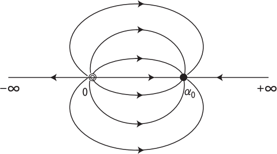
Figure 3: Lines of RG flow in the complex $\alpha$ plane for increasing $\rho$ ($\alpha_{0}>0$).

It is interesting to recognize that the lines of RG flow resemble the lines of force generated by a dipole. All lines of flow tend to $\alpha_{0}$, except for the one along the negative real axis that cannot go up nor down in the complex plane.

In (4.32) we found that $\alpha=0$ is a discontinuity for the integral of the spectral function of the gluon propagator. We can extend this observation to the complex $\alpha$ plane, and for this purpose we shall write down the sum rule for negative $\alpha$ and also for $\alpha+i\epsilon$:

$$\int dm^{2}\,\rho(m^{2},g^{2},\alpha,\mu) = 0\,,\ \ \ (\alpha<0)$$ (5.24)

$$\lim_{\epsilon\to 0}\int dm^{2}\,\rho(m^{2},g^{2},\alpha+i\epsilon,\mu) = \frac{\alpha}{\alpha_{0}}\,,\ \ \ (\alpha<0)\,.$$ (5.25)

This shows that there is a discontinuity in the integral of the spectral function when $\alpha$ approaches the negative real axis.

QED

The situation is completely different in QED. First of all, a gauge-invariant two-point function

$$\langle F_{\lambda\sigma}(x),F_{\mu\nu}(y)\rangle$$ (5.26)

can be expressed in terms of the transverse part of the photon propagator so that the photon mass that appears as the pole of this expression is physical. QED is characterized by Ward’s identity

$$Z_{1}=Z_{2}\,,$$ (5.27)

which is expressed in terms of anomalous dimensions by

$$\beta(e)=e\gamma_{V}(e)\,,$$ (5.28)

from which we can derive

$$\frac{d}{d\rho}[\bar{e}^{2}(\rho)\,\bar{\alpha}(\rho)]=0\,.$$ (5.29)

As mentioned already, the spectral function $\rho(m^{2})$ does not depend on $\alpha$, nevertheless, we have the sum rule:

$$Z_{3}^{-1}=\int dm^{2}\,\rho(m^{2})=\frac{\alpha}{\alpha_{\infty}}>1\,.$$ (5.30)

The only consistent choice of $\alpha_{\infty}$ that makes $Z_{3}$ independent of $\alpha$ is $\alpha_{\infty}=0$, and $e^{2}_{\infty}=\infty$ follows from (5.29).

In this case, $\alpha_{\infty}$ is the only asymptotic limit that is attractive, and there is only one equivalence class of gauges in QED. Furthermore, $e_{\infty}=\infty$ signifies that $\gamma_{V}(e)$ is positive definite, and the expression

$$\frac{\bar{\alpha}(\rho)}{\alpha}=\exp\left[-2\int_{0}^{\rho}d\rho^{\prime}\,\bar{\gamma}_{V}(\rho^{\prime})\right]$$ (5.31)

is real and decreases with increasing $\rho$. Then, the lines of RG flow in QED are shown in Fig. 4.

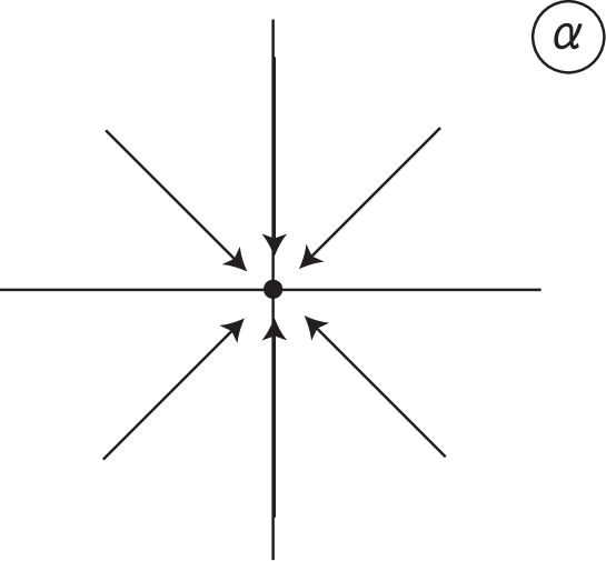
Figure 4: Lines of RG flow in the complex $\alpha$ plane for increasing $\rho$ (QED).

Here the lines of RG flow resemble the lines of force generated by a monopole.

In QED we have only one equivalence class of gauges and the massless photon is physical and observable. In this case we have

$$Z_{3}^{-1}=\infty$$ (5.32)

and charge confinement is not realized.

6 Conclusions

We may summarize what we have done in this paper in connection with the results obtained in a series of papers on this subject [5, 6, 11, 12].

1) Color $SU(3)$ symmetry

For color confinement we need an exact non-Abelian gauge symmetry. If this symmetry is broken, a color singlet state is forced to mix with colored states and consequently color cannot be confined. Mathematically, the original form of the condition for color confinement was given by the absence of the massless spin zero component in the current $\delta\bar{\delta}A_{\lambda}^{a}$, but breaking of color symmetry would induce the unwanted massless spin zero component in that current in the form of the Nambu-Goldstone boson. In Abelian gauge theories such as QED the massless spin zero component is always present, thereby preventing the charges from being confined.

2) Condition for Color Confinement

With the help of renormalization group we can show that a sufficient condition for color confinement can be cast in the form of Eq. (4.41), which formed the basis of our discussion in the present paper.

3) Evaluation of $Z_{3}$

Furthermore, with the help of renormalization group we can derive the identity (4.28) and can show with the help of asymptotic freedom that for negative choices of $\alpha$, eventually below a certain negative constant, $\alpha_{\infty}$ turn out to be $-\infty$, satisfying the condition (4.41) for confinement.

4) $S$-matrix in Confined QCD

By using gauge-independent Green’s functions we can express the $S$-matrix elements for hadronic reactions by applying the reduction formula [7]. The unitarity condition for the $S$-matrix between two hadronic states are expressed by Eq. (4.42), and confinement is characterized by the statement that the sum over the intermediate states is saturated by keeping only hadronic states, excluding colored particles such as quarks and gluons.

If confinement is realized in one gauge in the above sense, it is clearly realized also in all other gauges, since the $S$-matrix is gauge-independent. In this sense the concept of gauge-independence is a key factor in understanding confinement. The importance of gauge-independence or invariance has been stressed by many authors [14, 15, 16].

Acknowledgements

One of the authors (K.N.) is grateful to D.V. Shirkov for useful discussion on the subject and acknowledges the support by a Grant-in-Aid for Scientific Research from MEXT of Japan. Last but not least, we owe M. Chaichian his constant encouragement in pursuing this work.

References

- [1] C. Becchi, A. Rouet and R. Stora, Ann. Phys 98 (1976) 287.
- [2] M. Gell-Mann and F. E. Low, Phys. Rev. 95 (1954) 1300.
- [3] N. Bogoliubov and D. Shirkov, Introduction to the Theory of Quantized Fields, Wiley, New York, 1959.
- [4] D.V. Shirkov, Nucl. Phys. B 322 (1990) 425 and other related papers quoted therein.
- [5] K. Nishijima, Czech. J. Phys. 46 (1996) 1.
- [6] K. Nishijima and N. Takase, Int. J. Mod. Phys., A 11 (1996) 2281.
- [7] H. Lehmann, K. Symanzik and W. Zimmermann, Nuovo Cim. 1 (1955) 205.
- [8] D. J. Gross and F. Wilczek, Phys. Rev. Lett. 30 (1973) 1343.
- [9] H. D. Politzer, Phys. Rev. Lett. 30 (1973) 1346.
- [10] M. Chaichian and K. Nishijima, Eur. Phys. J. C 47 (2006) 737.
- [11] K. Nishijima, Int. J. Mod. Phys. A 9 (1994) 3799.
- [12] K. Nishijima, Int. J. Mod. Phys. A 10 (1995) 3155.
- [13] M. Chaichian and K. Nishijima, Eur. Phys. J. C 22 (2001) 463.
- [14] K. Fujikawa, B. W. Lee and A. I. Sanda, Phys. Rev. D 6 (1972) 2923.
- [15] G. ’t Hooft, Nucl Phys. B 138 (1978) 1.
- [16] R. P. Feynman, Nucl. Phys. B 188 (1981) 479.