Geometric entanglement witnesses and bound entanglement

Abstract

We study entanglement witnesses that can be constructed with regard to the geometrical structure of the Hilbert-Schmidt space, i.e. we present how to use these witnesses in the context of quantifying entanglement and the detection of bound entangled states. We give examples for a particular three-parameter family of states that are part of the magic simplex of two-qutrit states.

The determination whether a general quantum state is entangled or not is of utmost importance in quantum information. States of composite systems can be classified in Hilbert space as either entangled or separable. The geometric structure of entanglement is of high interest, particularly in higher dimensions. For $2\times 2$ bipartite qubits, the geometry is highly symmetric and very well known. In higher dimensions, like $3\times 3$ two-qutrit states, the structure of the corresponding Hilbert space is more complicated and less known. New phenomena like bound entanglement occur. In principle, all entangled states can be detected by the entanglement witness procedure. We construct in this Brief Report entanglement witnesses with regard to the geometric structure of the Hilbert-Schmidt space and explore a specific class of states, the three-parameter family of states. We discover by our method new regions of bound entanglement.

Let us recall some basic definitions we need in our discussion. We consider a Hilbert-Schmidt space ${\cal A}={\cal A}_{1}\otimes{\cal A}_{2}\otimes\ \ldots\ \otimes{\cal A}_{n}$ of operators acting on the Hilbert space of $n$ composite quantum systems - it is of dimension $d_{1}\times d_{2}\times\ \ldots\ \times d_{n}$ and $D:=d_{1}d_{2}\ldots d_{n}$. In Ref. Witte and Trucks (1999) a new geometric entanglement measure (which we call Hilbert-Schmidt measure) based on the Hilbert-Schmidt distance between density matrices is presented – and discussed in Ref. Ozawa (2000) – that is an instance of a distance measure (see Refs. Vedral et al. (1997); Vedral and Plenio (1998)). The entanglement of a state $\rho$ can be quantified (or “measured”) via the minimal Hilbert-Schmidt distance of the state to the convex and compact set of separable (disentangled) states $S$:

$$D(\rho):=\min_{\sigma\in S}\|\sigma-\rho\|\,.$$ (1)

It is defined on the Hilbert-Schmidt metric with a scalar product between operators that are elements of the Hilbert-Schmidt space ${\cal A}$: $\langle A,B\rangle:=\textnormal{Tr}A^{\dagger}B,\;A,B\in{\cal A}$ and the norm $\|A\|:=\sqrt{\langle A,A\rangle}\,$. Of course these definitions apply to density matrices (states of the quantum system), since they are operators of ${\cal A}$ with the properties $\rho^{\dagger}=\rho$, Tr$\rho=1$ and $\rho\geq 0$ (positive semidefinite operators).

Because the norm is continuous and the set of separable states $S$ is compact the minimum in Eq. (1) is attained for some separable state $\sigma_{0}$, $\min_{\sigma\in S}\|\sigma-\rho\|=\|\sigma_{0}-\rho\|\,$, which we call the nearest separable state to $\rho$. Clearly if $\rho\in S$ then $\sigma_{0}=\rho$ and $D(\rho)=0$. If $\rho$ is entangled, $\rho_{\rm{ent}}$, then $D(\rho)>0$ and $\sigma_{0}$ lies on the boundary of the set $S$. It is shown in Refs. Pittenger and Rubin (2002); Bertlmann et al. (2002); Pittenger and Rubin (2003); Bertlmann et al. (2005) that an operator

$$A_{\rm{opt}}=\sigma_{0}-\rho_{\rm{ent}}-\left\langle\sigma_{0},\sigma_{0}-\rho_{\rm{ent}}\right\rangle\mathbbm{1}_{\rm{D}}$$ (2)

defines a hyperplane including the state $\sigma_{0}$ that is tangent to $S$, and it has the properties

$$\left\langle\rho_{\rm{ent}},A_{\rm{opt}}\right\rangle=\textnormal{Tr}\,\rho_{\rm{ent}}A_{\rm{opt}} <0\,,$$ (3)

$$\left\langle\sigma,A_{\rm{opt}}\right\rangle=\textnormal{Tr}\,\sigma A_{\rm{opt}} \geq 0\quad\forall\sigma\in S\,.$$ (4)

It is clearly Hermitian and thus is an entanglement witness for the state $\rho_{\rm{ent}}$ Horodecki et al. (1996); Terhal (2000). Moreover, since the hyperplane is tangent to $S$ (Tr$\sigma_{0}A_{\rm{opt}}=0$) the operator $A_{\rm{opt}}$ (2) is called optimal entanglement witness. We call any entanglement witness that is constructed in the way of Eq. (2) – with any two states, not necessarily the nearest separable state – a geometric entanglement witness.

The crucial point lies in finding the nearest separable state: Once found, we can both quantify the entanglement of a state and construct an (even optimal) entanglement witness. But finding the nearest separable state is a hard task. A “guess-method”, that is a method to check if a good guess for the nearest separable state is indeed right, is presented in Ref. Bertlmann et al. (2005). Another way is to look for the nearest state that is positive under partial transposition (PPT) first. A method that finds the nearest PPT state in many cases is presented in Ref. Verstraete et al. (2002).

The PPT-criterion Peres (1996); Horodecki et al. (1996) is a necessary criterion for separability (sufficient for $2\times 2$ or $2\times 3$ dimensional Hilbert spaces): A separable state has to stay positive semidefinite under partial transposition – i.e. transposition in only one subsystem. Thus if a density matrix becomes indefinite under partial transposition, i.e. one or more eigenvalues are negative, it has to be entangled and we call it a NPT entangled state. But there exist entangled states that remain positive semidefinite – PPT entangled states – these are called bound entangled states, since they cannot be distilled to a maximally entangled state Horodecki (1997); Horodecki et al. (1998).

The set of all PPT states $P$ is convex and compact and contains the set of separable states. Thus the nearest separable state $\sigma_{0}$ can be replaced by the nearest PPT state $\tau_{0}$ for which the minimal distance to the set of PPT states is attained, $\min_{\tau\in P}\|\tau-\rho\|=\|\tau_{0}-\rho\|\,$. If $\rho$ is a NPT entangled state $\rho_{\rm{NPT}}$ and $\tau_{0}$ the nearest PPT state, then the operator

$$A_{\rm{PPT}}:=\tau_{0}-\rho_{\rm{NPT}}-\langle\tau_{0},\tau_{0}-\rho_{\rm{NPT}}\rangle\mathbbm{1}_{\rm{D}}$$ (5)

defines a tangent hyperplane to the set $P$ for the same geometric reasons as operator (2) and has to be an entanglement witness since $P\supset S$. In principle the entanglement of $\rho_{\rm{NPT}}$ can be measured in experiments that should verify Tr$A_{\rm{PPT}}\rho_{\rm{NPT}}<0$. If the state $\tau_{0}$ is separable, it has to be the nearest separable state $\sigma_{0}$ since the operator (5) defines a tangent hyperplane to the set of separable states. Therefore in this case $A_{\rm{PPT}}$ is an optimal entanglement witness, $A_{\rm{PPT}}=A_{\rm{opt}}$, and the Hilbert-Schmidt measure of entanglement can be readily obtained. If $\tau_{0}$ is not separable, that is PPT and entangled, it has to be a bound entangled state.

Unfortunately it is not trivial to check if the state $\tau_{0}$ is separable or not. It is hard to find evidence of separability, but it might be easier to reveal bound entanglement, not only for the state $\tau_{0}$ but for a whole family of states. A method to detect bound entangled states we are going to present.

Consider any PPT state $\rho_{\rm{PPT}}$ and the family of states $\rho_{\lambda}$ that lie on the line between $\rho_{\rm{PPT}}$ and the maximally mixed (and of course separable) state $\frac{1}{D}\mathbbm{1}_{\rm{D}}$,

$$\rho_{\lambda}:=\lambda\,\rho_{\rm{PPT}}+\frac{(1-\lambda)}{D}\mathbbm{1}_{\rm{D}}\,.$$ (6)

We can construct an operator $C_{\lambda}$ in the following way:

$$C_{\lambda}=\rho_{\lambda}-\rho_{\rm{PPT}}-\langle\rho_{\lambda},\rho_{\lambda}-\rho_{\rm{PPT}}\rangle\mathbbm{1}_{\rm{D}}\,.$$ (7)

If we can show that for some $\lambda_{\rm{min}}<1$ we have $\textnormal{Tr}\,\sigma C_{\lambda_{\rm{min}}}\geq 0$ for all $\sigma\in S$, $C_{\lambda_{\rm{min}}}$ is an entanglement witness and therefore $\rho_{\rm{PPT}}$ and all states $\rho_{\lambda}$ with $\lambda_{\rm{min}}<\lambda\leq 1$ are bound entangled (see Fig. 1).

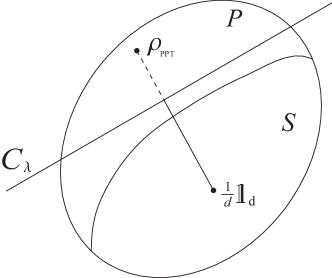
Figure 1: Sketch of the presented method to detect bound entanglement with the geometric entanglement witness $C_{\lambda}$. The dashed line indicates the detected bound entangled states $\rho_{\lambda}$ ($\lambda_{\rm{min}}<\lambda\leq 1$), states $\rho_{\lambda}$ with $0<\lambda\leq\lambda_{\rm{min}}$ can be separable or bound entangled (straight line).

As an example we introduce the following family of three-parameter two-qutrit states (dimension $3\times 3$ and $\mathbbm{1}:=\mathbbm{1}_{9}$):

$$\rho_{\alpha,\beta,\gamma}\;:=\;\frac{1-\alpha-\beta-\gamma}{9}\mathbbm{1}+\alpha P_{00}+\frac{\beta}{2}\left(P_{10}+P_{20}\right)+\frac{\gamma}{3}\left(P_{01}+P_{11}+P_{21}\right)\,,$$ (8)

where the parameters are constrained by the positivity requirement $\rho_{\alpha,\beta,\gamma}\geq 0$. The states $P_{nm}$ are projectors onto maximally entangled two-qutrit vector states Narnhofer (2006) – the Bell states

$$P_{nm}:=(U_{nm}\otimes\mathbbm{1})|\phi^{+}_{3}\rangle\langle\phi^{+}_{3}|(U_{nm}^{\dagger}\otimes\mathbbm{1})\,,$$ (9)

where $|\phi^{+}_{3}\rangle$ denotes the maximally entangled state $\left|\phi^{+}_{d}\right\rangle=\frac{1}{\sqrt{d}}\,\sum_{j}\left|j\right\rangle\otimes\left|j\right\rangle$ and $U_{nm}$ represent the Weyl operators $U_{nm}=\sum_{k=0}^{d-1}e^{\frac{2\pi i}{d}\,kn}\,|k\rangle\langle(k+m)\,\textrm{mod}\,d|$ with $n,m=0,1,\ldots,d-1$ (here $d_{1}=d_{2}=d$).

The states (8) lie in the magic simplex of two-qutrit states which is the set of all two-qutrit states that can be written as a convex combination of the projectors $P_{nm}$ (9). Viewing the indices $nm$ as points in a discrete phase space the magic simplex reveals a high symmetry that makes its geometry much more evident (see Refs. Baumgartner et al. (2006, 2007, )).

For $\gamma=0$ the geometry of the states (8) becomes rather simple. It is shown in Ref. Baumgartner et al. (2006) that all states of this two-parameter family are either NPT entangled or separable, that is, all PPT states coincide with the separable states. Therefore we can easily calculate the Hilbert-Schmidt measure with help of our entanglement witness (2).

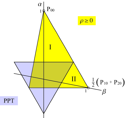
Figure 2: Illustration of states $\rho_{\alpha,\beta}$ (8) ($\gamma=0$) and their partial transposition. The regions I and II label the regions where the states are NPT entangled, they are PPT and separable in the overlap with the region of PPT points. The PPT points become semipositive under partial transposition.

In the two-dimensional picture (see Fig. 2) we can easily acquire the nearest points on the border of the separable states – here equal to the PPT states – to the points in the regions I and II that correspond to the entangled states: For region I the nearest point to $(\alpha,\beta)$ is $(\frac{1}{4}+\frac{1}{8}\beta,\beta)$ which characterizes a state $\tilde{\sigma}_{\beta}$ of the family (8). For region II the nearest point is $(\frac{1}{24}(-2+20\alpha+5\beta),\frac{1}{6}(2+4\alpha+\beta))$ which corresponds to a state $\tilde{\sigma}_{\alpha,\beta}$. According to Ref. Bertlmann et al. (2005) we can check if a proposed separable state $\tilde{\sigma}$ is the nearest separable one to an entangled state $\rho$ (considering the geometry of all states) by checking if the operator

$$C=\tilde{\sigma}-\rho-\langle\tilde{\sigma},\tilde{\sigma}-\rho\rangle\mathbbm{1}_{\rm{D}}$$ (10)

is an entanglement witness. To do so let us first state the following Lemma:

Lemma 1.

For any Hermitian operator $C$ of a bipartite Hilbert-Schmidt space of dimension $d\times d$ that is of the form

$$C\;=\;a\left((d-1)\,\mathbbm{1}_{\rm{d^{2}}}\,+\,\sum_{n,m=0}^{d-1}c_{nm}\,U_{nm}\otimes U_{-nm}\right),\quad a\in\mathbbm{R}^{+},\ c_{nm}\in\mathbbm{C}$$ (11)

the expectation value for all separable states is positive,

$$\langle\rho,C\rangle\,\geq\,0\quad\forall\,\rho\in S\,,\quad\mbox{{if}}\quad|c_{nm}|\,\leq\,1\quad\forall\,n,m\,.$$ (12)

Proof. Any bipartite separable state can be decomposed into Weyl operators as

$$\rho\;=\; \sum_{k}p_{k}\ \frac{1}{d^{2}}\Big{(}\mathbbm{1_{\rm{d}}}\otimes\mathbbm{1_{\rm{d}}}\,+\,\sum_{n,m=0}^{d-1}\sqrt{d-1}\,n_{nm}^{k}\,U_{nm}\otimes\mathbbm{1_{\rm{d}}}\,+\,\sum_{l,k=0}^{d-1}\sqrt{d-1}\,m_{lk}^{k}\,\mathbbm{1_{\rm{d}}}\otimes U_{lk}$$

$$+\sum_{n,m,l,k=0}^{d_{1}-1}(d-1)\,n_{nm}^{k}m_{lk}^{k}U_{nm}\otimes U_{lk}\Big{)}\,,$$

$$n_{nm}^{k},m_{lk}^{k}\in\mathbbm{C}\,,\;\quad\left|\vec{n}^{k}\right|\leq 1\,,\quad\left|\vec{m}^{k}\right|\leq 1\,,\quad\ p_{k}\geq 0,\;\sum_{k}p_{k}=1\,,$$ (13)

where we define $\left|\vec{n}^{k}\right|^{2}:=\sum_{nm}n_{nm}^{*}n_{nm}$. We call a decomposition (Geometric entanglement witnesses and bound entanglement) Bloch vector form of the density matrix. Note that for $d>2$ not any vector with complex components represents a Bloch vector (a quantum state), details can be found in Ref. Bertlmann and Krammer .

Performing the trace we obtain (keeping notation $\rho^{\dagger}$ formula (14) becomes more evident)

$$\langle\rho,C\rangle\;=\;\textnormal{Tr}\rho^{\dagger}\,C\;=\;\sum_{k}p_{k}\left((d-1)a\left(1\,+\,\sum_{n,m}c_{nm}n_{nm}^{*k}m_{-nm}^{*k}\right)\right)\,,$$ (14)

and using the restriction $|c_{nm}|\,\leq\,1\;\;\forall\,n,m$ we have

$$\left|\sum_{n,m}c_{nm}n_{nm}^{*k}m_{-nm}^{*k}\right|\;\leq\;\sum_{n,m}|n_{nm}^{k}||m_{-nm}^{k}|\;\leq\;1\,,$$ (15)

and since the convex sum of positive terms stays positive we get $\langle\rho,C\rangle\;\geq\;0\;\;\forall\rho\in S\,.\ \Box$

We set up the operators $C_{I},C_{II}$ for the two regions, respectively, according to Eq. (10) and write them in terms of Weyl operators normalized by $\|\tilde{\sigma}-\rho\|$ for convenience,

$$C_{I}=\frac{1}{6\sqrt{2}}(2\mathbbm{1}-U_{1}-U_{2})\,,\quad C_{II}=\frac{1}{6\sqrt{2}}(2\mathbbm{1}+U_{1}-U_{2})\,,$$ (16)

where

$$U_{1} :=U_{01}\otimes U_{01}+U_{02}\otimes U_{02}+U_{11}\otimes U_{-11}+U_{12}\otimes U_{-12}+U_{21}\otimes U_{-21}+U_{22}\otimes U_{-22}\,,$$

$$U_{2} :=U^{I}_{2}+U^{II}_{2}\qquad\mbox{with}\quad U^{I}_{2}:=U_{10}\otimes U_{-10}\,,\quad U^{II}_{2}:=U_{20}\otimes U_{-20}\,.$$ (17)

Both operators $C_{I}$ and $C_{II}$ satisfy Eq. (12) of Lemma 1. Due to the construction of the operators, Eq. (3) is satisfied for any entangled states $\rho_{\alpha,\beta}$ in the regions I and II. Consequently $C_{I}$ and $C_{II}$ are entanglement witnesses and therefore $\tilde{\sigma}_{\beta}$ and $\tilde{\sigma}_{\alpha,\beta}$ are the nearest separable states $\sigma_{0;\,\beta}$ and $\sigma_{0;\,\alpha,\beta}$. The corresponding Hilbert-Schmidt measures of the entangled two-parameter states $\rho_{\alpha,\beta}$ are

$$D_{I}(\rho_{\alpha,\beta}^{\rm{ent}})=\|\sigma_{0;\,\beta}-\rho_{\alpha,\beta}^{\rm{ent}}\|=\frac{2\sqrt{2}}{3}\left(\alpha-\frac{1}{4}-\frac{1}{8}\beta\right)\,.$$ (18)

$$D_{II}(\rho_{\alpha,\beta}^{\rm{ent}})=\|\sigma_{0;\,\alpha,\beta}-\rho_{\alpha,\beta}^{\rm{ent}}\|=\frac{2\sqrt{2}}{6}\left(-\alpha-\frac{1}{2}+\frac{5}{4}\beta\right)\,.$$ (19)

Note that the measures can also be viewed as a maximal violation of the entanglement witness inequality (4), as it is shown in detail in Refs. Bertlmann et al. (2002, 2005).

Another way to arrive at the nearest separable states for the two-parameter states is to calculate the nearest PPT states with the method of Ref. Verstraete et al. (2002) first and then check if the gained states are separable. If we do so we obtain for the nearest PPT states the states $\tilde{\sigma}_{\beta}$ and $\tilde{\sigma}_{\alpha,\beta}$ we have found with our “guess” method, we know from Ref. Baumgartner et al. (2006) that these states are separable and therefore they have to be the nearest separable states.

Let us return to the family of three-parameter states $\rho_{\alpha,\beta,\gamma}$ (8). For $\gamma\neq 0$ it is not trivial to find the nearest separable states since the PPT states do not necessarily coincide with the separable states. But we can use our geometric entanglement witness (7) to detect bound entanglement.

In Ref. Horodecki et al. (1999) the following one-parameter family of two-qutrit states was introduced:

$$\rho_{b}\;=\;\frac{2}{7}\left|\phi_{+}^{3}\right\rangle\left\langle\phi_{+}^{3}\right|+\frac{b}{7}\,\sigma_{+}+\frac{5-b}{7}\,\sigma_{-}\,,\qquad 0\leq b\leq 5\,,$$ (20)

where

$$\sigma_{+}:=\ 1/3\left(\left|01\right\rangle\left\langle 01\right|+\left|12\right\rangle\left\langle 12\right|+\left|20\right\rangle\left\langle 20\right|\right)\,,$$

$$\sigma_{-}:=\ 1/3\left(\left|10\right\rangle\left\langle 10\right|+\left|21\right\rangle\left\langle 21\right|+\left|02\right\rangle\left\langle 02\right|\right)\,.$$ (21)

Let us call this family of states Horodecki states. Interestingly, the states (20) are part of the three-parameter family (8), namely $\rho_{b}\equiv\rho_{\alpha,\beta,\gamma}\,,\;\;\mbox{with}\;\;\alpha=(6-b)/21\,,\;\beta=-2b/21\,,\;\gamma=(5-2b)/7$ and thus lie in the magic simplex. Testing the partial transposition we find that the Horodecki states (20) are NPT for $0\leq b<1$ and $4<b\leq 5$ and PPT for $1\leq b\leq 4$. In Ref. Horodecki et al. (1999) it is shown that the states are separable for $2\leq b\leq 3$ and bound entangled for $3<b\leq 4$.

We now want to pursue the following idea: Starting from a PPT and entangled – bound entangled – Horodecki state $\rho_{b}^{\rm{BE}}$ we construct operators in the way of Eq. (7) and try to find bound entanglement on the line between $\rho_{b}^{\rm{BE}}$ and the maximally mixed state – see Fig. 1.

For a geometric picture of the three-parameter family of states $\rho_{\alpha,\beta,\gamma}$ we can fix values of $\gamma$ and draw two-dimensional slices (see Fig. 3).

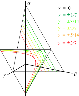
Figure 3: The states $\rho_{\alpha,\beta,\gamma}$ are depicted with slices of the three-dimensional parameter space for fixed values of $\gamma$. The curved borders of the PPT regions for $\gamma\neq 0$ are hyperbolae that result from intersecting a cone of PPT points with the planes of constant $\gamma$. The slices for positive and negative $\gamma$ overlap. All parameter axes are chosen non-orthogonal such that they become orthogonal to the boundary of the positivity region in order to reproduce the symmetry of the magic simplex.

Translated to values of $\gamma$ the states $\rho_{b}=\rho_{\alpha,\beta,\gamma}$ are bound entangled for $-3/7\leq\gamma<-1/7$ and in each slice of this region there is exactly one point that corresponds to the bound entangled Horodecki state, namely $\left(\alpha=(1+\gamma)/6\,,\,\beta=(-5+7\gamma)/21\right)$. The one-parameter line of the states $\rho_{b}$ therefore cuts through the slices of fixed $\gamma$ and lies on the boundary of the states (8).

For a fixed $\gamma$ the operator $C_{\gamma,\lambda}$ (7) has the following form:

$$C_{\gamma,\lambda}\;=\;\rho_{\lambda}-\rho_{b}^{\rm{BE}}-\langle\rho_{\lambda},\rho_{\lambda}-\rho_{b}^{\rm{BE}}\rangle\mathbbm{1}\;=\;a(2\,\mathbbm{1}+c_{1}U_{1}+c_{2}U^{I}_{2}+c^{\star}_{2}U^{II}_{2})\,,$$

$$\mbox{with}\quad a=-\frac{1+3\gamma^{2}}{36}\lambda(\lambda-1),\;c_{1}=-\frac{8}{7\lambda(1+3\gamma^{2})},\;c_{2}=\frac{2(1-7\sqrt{3}\gamma\,i)}{7\lambda(1+3\gamma^{2})}\,,$$ (22)

and $\rho_{\lambda}$ represents the line of states

$$\rho_{\lambda}\;=\;\lambda\rho_{b}^{\rm{BE}}+\frac{1-\lambda}{9}\mathbbm{1}\,.$$ (23)

It is convenient to define functions $f_{1}(\gamma,\lambda):=|c_{1}|$ and $f_{2}(\gamma,\lambda):=|c_{2}|\,$. We are interested to find the minimal $\lambda$ for a particular $\gamma$ which is attained at $\max\{f_{1}(\gamma,\lambda),f_{2}(\gamma,\lambda)\}=1$, i.e. the minimal $\lambda$ such that $C_{\gamma,\lambda}$ (Geometric entanglement witnesses and bound entanglement) is necessarily an entanglement witness (see Lemma 1). There exist values of $\lambda$ with $\lambda<1$ such that $\max\{f_{1}(\gamma,\lambda),f_{2}(\gamma,\lambda)\}<1$ for $1/\sqrt{21}<|\gamma|\leq 3/7$. That means we are able to detect bound entangled states on lines (23) between the bound entangled Horodecki states and the maximally mixed state $\frac{1}{9}\mathbbm{1}$ until a value of $|\gamma|=1/\sqrt{21}$. These lines form a planar section of bound entangled states restricted by $\lambda_{\rm{min}}<\lambda\leq 1$. As a “side product” we are able to detect bound entanglement for the Horodecki states for $1\leq b<\frac{1}{6}(15-\sqrt{21})(\simeq 1.74)$ and $\frac{1}{6}(15+\sqrt{21})(\simeq 3.26)<b\leq 4$.

A detailed examination of the coefficient functions $f_{1}(\gamma,\lambda)$ and $f_{2}(\gamma,\lambda)$ exhibits that for $1/\sqrt{21}<|\gamma|<\sqrt{5}/7$ we have $f_{1}>f_{2}$ and for $\sqrt{5}/7<|\gamma|\leq 3/7$ we have $f_{1}<f_{2}$ and equality $f_{1}=f_{2}$ at $\sqrt{5}/7$. The total minimum is $\lambda_{\rm{min}}^{\rm{tot}}=7/8=0.875$, i.e. the minimal $\lambda$ that can be reached such that all states $\rho_{\lambda}$ (23) are detected to be bound entangled for $\lambda_{\rm{min}}^{\rm{tot}}<\lambda\leq 1$. It is attained for $|\gamma|=\sqrt{5}/7$ or $b=\frac{1}{2}(5-\sqrt{5})\simeq 1.38$ and $b=\frac{1}{2}(5+\sqrt{5})\simeq 3.62$.

Summarizing, the magic simplex contains three classes of states: NPT entangled states, separable states but also PPT entangled or bound entangled states. We have found such bound entangled states analytically in a quite large region of the magic simplex. Our method works very well for the examples presented and is geometrically very intuitive. However, we cannot detect in these examples the border between bound entangled and separable states. The reason is that condition $|c_{nm}|\,\leq\,1\;\;\forall\,n,m$ in Eq. (12) is only sufficient for $C$ being an entanglement witness and not necessary. There is generally still no operational method for detecting the nearest separable states.

References

Witte and Trucks (1999)
C. Witte and
M. Trucks,
Phys. Lett. A 257,
14 (1999).
Ozawa (2000)
M. Ozawa,
Phys. Lett. A 268,
158 (2000).
Vedral et al. (1997)
V. Vedral,
M. B. Plenio,
M. A. Rippin,
and P. L.
Knight, Phys. Rev. Lett.
78, 2275 (1997).
Vedral and Plenio (1998)
V. Vedral and
M. B. Plenio,
Phys. Rev. A 57,
1619 (1998).
Pittenger and Rubin (2002)
A. O. Pittenger
and M. H. Rubin,
Linear Algebr. Appl. 346,
75 (2002).
Bertlmann et al. (2002)
R. A. Bertlmann,
H. Narnhofer,
and W. Thirring,
Phys. Rev. A 66,
032319 (2002).
Pittenger and Rubin (2003)
A. O. Pittenger
and M. H. Rubin,
Phys. Rev. A 67,
012327 (2003).
Bertlmann et al. (2005)
R. A. Bertlmann,
K. Durstberger,
B. C. Hiesmayr,
and P. Krammer,
Phys. Rev. A 72,
052331 (2005).
Horodecki et al. (1996)
M. Horodecki,
P. Horodecki,
and
R. Horodecki,
Phys. Lett. A 223,
1 (1996).
Terhal (2000)
B. M. Terhal,
Phys. Lett. A 271,
319 (2000).
Verstraete et al. (2002)
F. Verstraete,
K. Audenaert,
and B. D. Moor,
J. Mod. Opt. 49,
1277 (2002).
Peres (1996)
A. Peres,
Phys. Rev. Lett. 77,
1413 (1996).
Horodecki (1997)
P. Horodecki,
Phys. Lett. A 232,
333 (1997).
Horodecki et al. (1998)
M. Horodecki,
P. Horodecki,
and
R. Horodecki,
Phys. Rev. Lett. 80,
5239 (1998).
Narnhofer (2006)
H. Narnhofer,
J. Phys. A: Math. Gen. 39,
7051 (2006).
Baumgartner et al. (2006)
B. Baumgartner,
B. C. Hiesmayr,
and
H. Narnhofer,
Phys. Rev. A 74,
032327 (2006).
Baumgartner et al. (2007)
B. Baumgartner,
B. C. Hiesmayr,
and
H. Narnhofer,
J. Phys. A: Math. Theor. 40,
7919 (2007).
(18)
B. Baumgartner,
B. C. Hiesmayr,
and
H. Narnhofer,
arXiv:0705.1403.
(19)
R. A. Bertlmann
and P. Krammer,
to appear (or see arXiv:0706.1743).
Horodecki et al. (1999)
P. Horodecki,
M. Horodecki,
and
R. Horodecki,
Phys. Rev. Lett 82,
1056 (1999).