Numerical study of metastable states in the $T=0$ RFIM

Abstract

We study numerically the number of single-spin-flip stable states in the $T=0$ Random Field Ising Model (RFIM) on random regular graphs of connectivity $z=2$ and $z=4$ and on the cubic lattice. The annealed and quenched complexities (i.e. the entropy densities) of the metastable states with given magnetization are calculated as a function of the external magnetic field. The results show that the appearance of a (disorder-induced) out-of-equilibrium phase transition in the magnetization hysteresis loop at low disorder can be ascribed to a change in the distribution of the metastable states in the field-magnetization plane.

I Introduction

At low temperature, disordered systems may be trapped in long-lived metastable states separated by large energy barriers that make relaxation to thermal equilibrium unlikely on experimental time scales. As a consequence, these systems, when driven by an external force, display a jerky and hysteretic behavior which is associated to irreversible jumps between the metastable states, events that are called avalanches. The out-of-equilibrium behavior is thus dictated by the properties of the local minima in the energy (or free-energy) landscape and it would be useful to know a priori their number and energy, or, in the case of magnetic systems, their magnetization. However, such a computation is a nontrivial task, even when the metastable states can be clearly identified, as it is the case at zero temperature or in mean-field models. Consider for instance the ferromagnetic Random Field Ising Model (RFIM) at $T=0$ which is a simple prototype of a spin system with avalanche behavior and has been extensively studied in recent years Sethna_review2004 . In this case, one would like to relate the hysteretic response of the system to an externally varying magnetic field to the distribution of the metastable states in the field-magnetization plane. In general, one expects the typical number of metastable states to scale exponentially with the system size inside the saturation hysteresis loop and to vanish outsideDetcheverry2005 . At low disorder, however, the existence of an out-of-equilibrium phase transition, characterized by a macroscopic jump in the hysteresis loop Sethna1993 , strongly suggests that the typical number of states also vanishes in some region inside the loop, as depicted schematically in Fig. 1(b). This feature may also explain the behavior observed when the system is driven by the magnetization instead of the magnetic fieldIlla2006a ; Illa2006b .

Figure 1: Putative distribution of the metastable states in the field-magnetization plane for the $T=0$ RFIM on the cubic lattice (or the Bethe lattice with $z=4$): (a) strong disorder regime (b) low disorder regime. The number of single-spin-flip stable states scales exponentially with the system size in the shaded region and is zero outside. The solid curve is the associated magnetization hysteresis loop. (Color on line.)

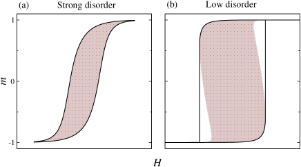
In a recent paperDetcheverry2005 , this issue was investigated analytically in the case of the RFIM on random regular graphs of fixed connectivity $z$ (akin to the Bethe lattice Mezard2001 ) for which the out-of-equilibrium phase transition occurs when $z\geq 4$ Dhar1997 . The annealed complexity $\Sigma_{A}(m;H)$ and the quenched complexity $\Sigma_{Q}(m;H)$ of the single-spin-flip stable states (i.e., the entropy densities associated to the average and typical number of states, $\overline{{\cal N}(m;H)}$ and $\exp[\overline{\ln{\cal N}(m;H)}]$, respectively) were studied as a function of the magnetization (per spin) $m$ and the external field $H$. The quenched complexity $\Sigma_{Q}(m;H)$, however, could only be obtained analytically for $z=2$ (i.e., in one dimension) and therefore the relationship between the phase transition in the hysteresis loop and the distribution of the typical states could not be investigated. On the other hand, $\Sigma_{A}(m;H)$ was computed for several values of $z$ but it was shown that its behavior does not reflect the typical behavior of the system; the difference may even be qualitative as for the change in the concavity of $\Sigma_{A}(m;H)$ which already occurs for $z=3$.

In the present work, we revisit the problem by performing numerical computations of $\Sigma_{A}(m,H)$ and $\Sigma_{Q}(m,H)$ on both random graphs and the cubic lattice. Since exact enumeration is only possible for systems of very small size, we also use more sophisticated statistical methods that allow us to consider larger systems and to make sensible extrapolations of the data to the thermodynamic limit despite the fact that the number of metastable states grows exponentially. The case $z=2$ for which complete analytical results are available is used as a benchmark.

The rest of the paper is organized as follows. In section II, we introduce the model, define the quantities that we want to compute, and briefly recall the main results of Ref. Detcheverry2005, . In section III, we explain how to properly define the complexities in finite systems, and, in section IV, we describe the numerical methods. The results for the $z=2$ random graphs are presented in section V and those for $z=4$ in section VI. The case of the cubic lattice, for which no analytical treatment is possible, is studied in section VII. Finally, in section VIII, we give some general remarks and conclude.

II Model

The RFIM is defined as a set of $N$ Ising spins $\{s_{i}=\pm 1,i=1,\dots,N\}$ placed on the vertices of a graph, with Hamiltonian

$${\cal H}=-\frac{J}{2}\sum_{i,j=1}^{N}n_{ij}s_{i}s_{j}-H\sum_{i=1}^{N}s_{i}-\sum_{i=1}h_{i}s_{i}.$$ (1)

$J$ is a ferromagnetic coupling constant (we take $J=1$ in the simulations) and $n_{ij}$ is a connectivity matrix that defines the topology of the graph ($n_{ij}=1$ if the vertices $i$ and $j$ are connected and $0$ otherwise). In the following we shall consider either random regular graphs with fixed connectivity $z=2$ and $z=4$ or the $3d$ cubic lattice. $H$ is a uniform external field and the quenched local fields $h_{i}$ are independent random variables drawn from a Gaussian probability distribution with zero mean and standard deviation $\Delta$ which parametrizes the amount of disorder in the system.

Hysteresis and avalanches in the RFIM have been extensively studied in the past years using the standard zero-temperature Glauber dynamicsSethna1993 ; Perkovic1999 ; PerezReche2003 ; Colaiori2004 . A state is then (meta)stable when its energy cannot be decreased by flipping a single spin. Although more general dynamics may be also considered, in which a configuration is stable if its energy cannot be decreased by flipping any subset of $1,2,...,k$ spinsNewman-Stein1999 , we shall only focus on the 1-spin-flip stable states that we simply call metastable (all other states are thus unstable with respect to the dynamics)

From Eq. (1), the change in the energy due to the flip of a single spin $s_{i}$ is

$$\Delta{\cal H}(s_{i}\rightarrow-s_{i})=2s_{i}f_{i},$$ (2)

where $f_{i}=J\sum_{j\neq i}n_{ij}s_{j}+h_{i}+H$ is the effective local field acting on $s_{i}$. The sum extends over the $z$ spins connected with $s_{i}$ (because the random field distribution is continuous, the probability of having $f_{i}=0$ is zero). According to Eq. (2), all the spins $s_{i}$ in a metastable configuration are aligned with their local field, i.e.,

$$s_{i}f_{i}>0.$$ (3)

As will be discussed below, it is also useful to introduce a “misalignment” parameter $\mu$ ($0\leq\mu\leq 1$) defined as

$$\mu=\frac{1}{N}\sum_{i=1}^{N}\Theta(-s_{i}f_{i}),$$ (4)

where $\Theta(x)$ is the Heaviside step function ($\Theta(x)=1$ if $x>0$ and $0$ if $x<0$). $\mu$ is the fraction of spins in a given configuration that are not aligned with their local field (metastable states thus correspond to $\mu=0$).

In the following, the two quantities that describe macroscopically a disorder realization are $\hat{\cal N}(m,\mu;H)$, the number of states at field $H$ with magnetization $m=(1/N)\sum_{i}s_{i}$ and misalignment $\mu$, and ${\cal N}(m;H)=\hat{\cal N}(m,0;H)$, the number of metastable states with magnetization $m$. These quantities are averaged over a large number of samples characterized by a different set of random fields and random graphs. Since both $\overline{{\cal N}(m;H)}$, the average number of metastable states, and $\exp[\overline{\ln{\cal N}(m;H)}]$, the typical number, are expected to scale exponentially with $N$ in some region of the $H-m$ plane, the interesting quantities are the corresponding annealed and quenched complexities

$$\Sigma^{\infty}_{A}(m;H)=\lim_{N\rightarrow\infty}\frac{1}{N}\ln\overline{{\cal N}(m;H)},$$ (5)

$$\Sigma^{\infty}_{Q}(m;H)=\lim_{N\rightarrow\infty}\frac{1}{N}\overline{\ln{\cal N}(m;H)},$$ (6)

where the superscript ‘$\infty$’ indicates that these quantities refer to the thermodynamic limit. As shown in Ref. Detcheverry2005, , the probability of finding metastable states outside the average hysteresis loop vanishes when $N\rightarrow\infty$. Accordingly, $\Sigma^{\infty}_{Q}(m;H)=-\infty$ (or is not defined) in this region whereas $\Sigma^{\infty}_{A}(m;H)$ may be positive because of the existence of nontypical metastable states. In other words, the contour $\Sigma^{\infty}_{A}(m;H)=0$ overestimates the size of the actual hysteresis loop. The situation inside the loop is more complicated, depending on the connectivity $z$ of the random graphs (or the spatial dimension) and the disorder strength. For $z=2$ (or in one dimension), $\Sigma^{\infty}_{A}$ and $\Sigma^{\infty}_{Q}$ are concave functions of $H$ and $m$ for all values of $\Delta$. On the other hand, for $z\geq 3$ and $\Delta$ small enough, $\Sigma^{\infty}_{A}$ becomes a nonmonotonic function of $m$ in some range of the field (Fig. 6 in Ref. Detcheverry2005, ) and $m_{A}^{\infty}(H)$, the (annealed) average magnetization of the states (corresponding to the maxima of $\Sigma^{\infty}_{A}(m;H)$), may display a discontinuity (Fig. 9 in Ref. Detcheverry2005, ). It is likely that the same is true on euclidean lattices in $3$ and higher dimensions. The corresponding behavior of $\Sigma^{\infty}_{Q}(m;H)$ is still unknown but, as discussed in Ref. Detcheverry2005, , the existence of a jump in the hysteresis loop at the coercive field (for $z\geq 4$ or $d\geq 3$ at low disorder) suggests that the curve $\Sigma^{\infty}_{Q}(m;H)=0$ has a reentrant part, as depicted in Fig. 1(b). This implies that $\Sigma^{\infty}_{Q}(m;H)$ has at least two maxima as a function of $m$ in a certain range of the field. It is also possible that the typical magnetization of the metastable states (corresponding to the maximum of $\Sigma^{\infty}_{Q}(m;H)$) has a discontinuity at a certain value of $H$. This is the general scenario that we try to confirm numerically in the present work.

III Definition of the complexities in finite-size systems

Since numerical simulations are performed in finite systems, one must define the corresponding $N$-dependent complexities in such a way that one can properly extrapolate the results to the thermodynamic limit.

It is quite natural to define the annealed complexity in finite systems as

$$\Sigma_{A}(m;H,N)=\frac{1}{N}\ln\overline{{\cal N}(m;H,N)},$$ (7)

so that the average number of metastable states is just $\overline{{\cal N}(m;H,N)}=\exp[N\Sigma_{A}(m;H,N)]$. A similar definition for the quenched complexity would be $\Sigma_{Q}(m;H,N)=(1/N)\overline{\ln{\cal N}(m;H,N)}$. This is not convenient, however, because the average of the logarithm diverges as soon as ${\cal N}(m;H,N)$ is zero in some sample, a situation that always occurs in a system of small size. One could imagine to circumvent the problem by arbitrarily setting $\ln({\cal N}(m;H,N))=0$ in this case (see, e.g., Ref. Cherrier-Dean-Lefevre2003, ). This should be unimportant in the thermodynamic limit since it concerns a number of states that is nonexponential in system size. However, we recall that we are especially interested in the region where the quenched complexity is very small and vanishes when $N\rightarrow\infty$. This procedure would thus introduce an unacceptable bias. The alternative solution that we propose is inspired by the analytical calculation of Ref. Detcheverry2005, , introducing the function $\Lambda_{\alpha}(g;H,N)$ defined by the following Legendre-Fenchel transform

$$\Lambda_{\alpha}(g;H,N)=\max_{m}\left\{\frac{1}{N}\ln{\cal N}_{\alpha}(m;H,N)+gm\right\},$$ (8)

where $g\in\mathbbmss{R}$ (we provisionally add the subscript $\alpha$ to recall that ${\cal N}(m;H,N)$ is sample-dependent). Note that we take the maximum of the expression inside the parenthesis with respect to $m$, which cures the problem of ${\cal N}_{\alpha}(m;H,N)$ being zero for some values of $m$.

Figure 2: Schematic behavior of the quenched complexity in the presence of a disorder-induced phase transition (e.g., on random graphs with $z=4$). (a) $\Sigma_{Q}(m;H)$ has a single maximum and is positive in the range $m_{-\infty}(H)\leq m\leq m_{+\infty}(H)$ (b) $\Sigma_{Q}(m;H)$ has two maxima and is positive in the range $m^{-}_{-\infty}(H)\leq m\leq m^{-}_{+\infty}(H)$ and $m^{+}_{-\infty}(H)\leq m\leq m^{+}_{+\infty}(H)$. $m$ and $\Sigma_{Q}(m;H)$ are parametrized by the Legendre variable $g$ which increases from $-\infty$ to $+\infty$ as indicated by the arrows.

Let us first consider the simplest situation where ${\cal N}_{\alpha}(m;H,N)$ has a single maximum (i.e., is concave). Then, for a given $g$, the function $(1/N)\ln{\cal N}_{\alpha}(m;H,N)+gm$ (or, equivalently, $e^{Ngm}{\cal N}_{\alpha}(m;H,N)$) has a single maximum at some magnetization $m_{\alpha}(g;H,N)$ and

$$\Lambda_{\alpha}(g;H,N)=\frac{1}{N}\ln{\cal N}_{\alpha}(m_{\alpha};H,N)+gm_{\alpha}.$$ (9)

The average over disorder yields

$$\Lambda(g;H,N)=\frac{1}{N}\overline{\ln{\cal N}_{\alpha}(m_{\alpha};H,N)}+gm$$ (10)

where $m(g;H,N)\equiv\overline{m_{\alpha}(g;H,N)}$. This leads to define the size-dependent quenched complexity as

$$\Sigma_{Q}(m;H,N)=\Lambda(g;H,N)-gm,$$ (11)

neglecting terms of order $1/N$ (as one expects that $m_{\alpha}$ deviates from it average value by terms of order $1/\sqrt{N}$) and considering both $m$ and $\Sigma_{Q}(m;H,N)$ as functions of the independent parameter $g$ through the relation $m=m(g;H,N)$. Clearly, one has $\Sigma_{Q}(m;H,N)\rightarrow\Sigma^{\infty}_{Q}(m;H)$ when $N\rightarrow\infty$, and $\Lambda$ and $\Sigma_{Q}$ are related by the standard Legendre relations $\partial\Lambda/\partial g=m$ and $\partial\Sigma_{Q}/\partial m=-g$ (neglecting again terms of order $1/N$ to derive the second relation). Varying $g$ from $-\infty$ to $+\infty$ then traces out the curve $\Sigma_{Q}(m;H,N)$ vs. $m$, as depicted schematically in Fig. 2(a). Moreover, one readily sees from Eq. (8) that the limit $g\rightarrow-\infty$ (resp. $g\rightarrow+\infty$) selects in each sample $\alpha$ the smallest (resp. largest) magnetization for which ${\cal N}_{\alpha}(m;H,N)$ is strictly positive. As shown in Ref. Detcheverry2005, , these two values of $m$ correspond to the lower and upper branch of the hysteresis loop, respectively. Therefore, the two curves obtained by plotting $m_{\pm\infty}(H,N)=\lim_{g\rightarrow\pm\infty}m(g;H,N)$ as a function of $H$ define the two branches of the average hysteresis loop. On the other hand, the typical (i.e. the most likely) value of the magnetization of the metastables states is described by the curve $m(g=0;H,N)$ which corresponds to the locus of the maximum of $\Sigma_{Q}$.

Now, consider the situation where ${\cal N}_{\alpha}(m;H,N)$ has two maxima associated to two separated lobes (see e.g. Fig. 12 in section VI.2). As discussed previously, such a situation is likely to occur in a certain range of $H$ when there exists an out-of-equilibrium phase transition, for instance on the $z=4$ Bethe lattice at low disorder. One expects the quenched complexity to display the same behavior, as depicted in Fig. 2(b), but this information cannot be extracted from Eqs. (8-11). In this case, it is convenient to treat the two maxima separately by introducing two Legendre-Fenchel transforms:

$$\Lambda_{\alpha}^{-}(g;H,N) =\max_{m<m_{th}}\left\{\frac{1}{N}\ln{\cal N}_{\alpha}(m;H,N)+gm\right\}$$

$$\Lambda_{\alpha}^{+}(g;H,N) =\max_{m>m_{th}}\left\{\frac{1}{N}\ln{\cal N}_{\alpha}(m;H,N)+gm\right\},$$ (12)

where $m_{th}$ is a certain threshold in magnetization which does not depend on the disorder realization and which is chosen so to lie between the two maxima for as many realizations as possible. In consequence, the size-dependent quenched complexity also splits into two parts,

$$\Sigma_{Q}^{-}\left(m;H,N)\right) =\Lambda^{-}(g;H,N)-gm^{-}$$

$$\Sigma_{Q}^{+}\left(m;H,N)\right) =\Lambda^{+}(g;H,N)-gm^{+}$$ (13)

where $m^{-}(g;H,N)\equiv\overline{m_{\alpha}^{-}(g;H,N)}$ and $m^{+}(g;H,N)\equiv\overline{m_{\alpha}^{+}(g;H,N)}$. It is again useful to consider the magnetization and the complexity $\Sigma_{Q}^{-}$ or $\Sigma_{Q}^{+}$ as functions of the independent parameter $g$ through the relations $m=m^{-}(g;H,N)$ or $m=m^{+}(g;H,N)$. Of course, one recovers the preceding formulas with only one function $\Lambda$ or $\Sigma_{Q}$ if $\mid m_{th}\mid>1$.

It is also interesting to consider the limits $g\rightarrow\pm\infty$. Now $m^{-}_{-\infty}(H,N)=\lim_{g\rightarrow-\infty}m^{-}(g;H,N)$ and $m^{+}_{+\infty}(H,N)=\lim_{g\rightarrow+\infty}m^{+}(g;H,N)$ correspond to the lower and upper branches of the hysteresis loop, respectively. On the other hand, in Eqs. (III), the limit $g\rightarrow+\infty$ (resp. $g\rightarrow-\infty$) selects in each sample the largest (resp. smallest) magnetization in the interval $[-1,m_{th}]$ (resp. $[m_{th},1]$) for which ${\cal N}_{\alpha}(m;H,N)>0$. Therefore, if $m^{-}_{\alpha}(g\rightarrow+\infty;H,N)<m_{th}<m^{+}_{\alpha}(g\rightarrow-\infty;H,N)$, there is a gap in magnetization for which ${\cal N}_{\alpha}(m;H,N)=0$. On the contrary, if $m^{-}_{\alpha}(g\rightarrow+\infty;H,N)=m^{+}_{\alpha}(g\rightarrow-\infty;H,N)$, the gap does not exist. In finite systems, the width of the gap fluctuates from one sample to another and the appropriate quantity to be analyzed is the average gap.

IV Numerical methods

We now detail the numerical methods that we have used to compute the number of metastable states as a function of the magnetization and the external field.

IV.1 Exact enumeration

The simplest method for counting the number of metastable states in a given disorder realization consists in generating all the spin configurations and selecting those which are metastable in a certain range of the field. To do this, we determine the interval of stability $[H_{min},H_{max}]$ of each configuration $\mathbf{s}=\{s_{i}\}$. Eq. (3) implies that a spin $s_{i}=+1$ (resp. $s_{i}=-1$) is stable as long as $H\geq-J\sum_{j\neq i}n_{ij}s_{j}-h_{i}$ (resp. $H\leq-J\sum_{j\neq i}n_{ij}s_{j}-h_{i}$). The fields $H_{min}$ and $H_{max}$ correspond to the two situations of marginal stability for $\mathbf{s}$, i.e.,

$$H_{min} =\max_{\{i|s_{i}=+1\}}\{-J\sum_{j\neq i}n_{ij}s_{j}-h_{i}\}$$ (14)

$$H_{max} =\min_{\{i|s_{i}=-1\}}\{-J\sum_{j\neq i}n_{ij}s_{j}-h_{i}\}\ .$$ (15)

Accordingly, configurations with $H_{min}\leq H_{max}$ are stable when $H$ is in the range $[H_{min},H_{max}]$. On the other hand, configurations with $H_{min}>H_{max}$ are always unstable since, whatever the value of $H$, at least the spin up corresponding to $H_{min}$ (or the spin down corresponding to $H_{max}$) is unstable. Since the total number of states grows like $2^{N}$, one of course cannot consider large systems. In the present work, the largest size investigated by this method is $N=26$ (with $5000$ disorder realizations). However, as will be seen below, some of the data can be reasonably extrapolated to the thermodynamic limit. Moreover, even in a small system, one can observe a clear connection between the shape of the hysteresis loop and the intervals of stability $[H_{min},H_{max}]$ of the metastable states.

Figure 3: Limits of stability $H_{min}$ (circles) and $H_{max}$ (crosses) of the metastable states in a single disorder realization on a random graph of size $N=26$: (a) $z=2$, $\Delta=1$, (b) $z=2$, $\Delta=2.5$ (c) $z=4$, $\Delta=1$ (d) $z=4$, $\Delta=2.5$.(Color on line.)

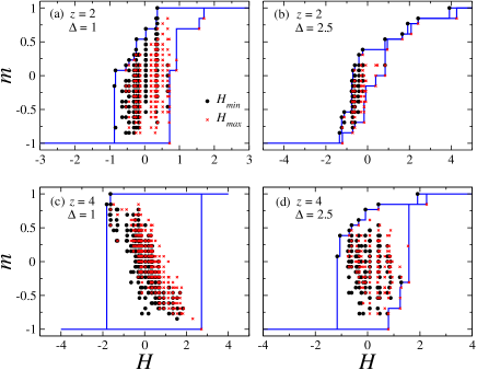
This is illustrated in Fig. 3 where we plot all the $H_{min}$ and $H_{max}$ obtained in a single sample (namely, a realization of the random fields on a random graph of size $N=26$) for different connectivities $z$ and/or values of $\Delta$. For a given overall magnetization $M=Nm$, there are in general several metastable states, each one characterized by a stability range $[H_{min},H_{max}]$ (for clarity, no link between $H_{min}$ and $H_{max}$ has been drawn in the figure.) The comparison of the distribution of these marginal fields in the $H$-$m$ plane with the corresponding saturation hysteresis loop shows that:

(i) There are no metastable states outside the loop, as expected theoreticallyDetcheverry2005 .

(ii) The hysteresis loop is a path in the $H$-$m$ plane that connects the extremal states, i.e. those which have the largest $H_{max}$ at a given $m$ (on the ascending branch) or the smallest $H_{min}$ (on the descending branch). An avalanche (for instance on the ascending branch) occurs between the extremal state $\mathbf{s}$ at $m$ and the extremal state $\mathbf{s}^{\prime}$ at $m^{\prime}>m$ when all the stable states with intermediate magnetization $m<m^{\prime\prime}<m^{\prime}$ have a $H_{max}$ which is smaller than $H_{max}(\mathbf{s})$. (In fact, this property is true in general for any pair of ordered states $\mathbf{s}$ and $\mathbf{s}^{\prime}>\mathbf{s}$note1 ). In other words, avalanches connect metastable states through a sequence of unstable (or, at most, marginally stable) intermediate configurations. For $z=2$ (and both $\Delta=1$ and $\Delta=2.5$), one can see in Figs. 3(a) and (b) that there are indeed some intermediate marginal states along the magnetization discontinuities of the hysteresis loop. In contrast, for $z=4$, marginal intermediate states are only observed when $\Delta$ is large enough (Fig. 3(d)). At low disorder (Fig. 3(c)), there exists a significant region inside the loop where there are no metastable states at all. This suggests that the discontinuity in the hysteresis loop in the thermodynamic limit is related to the existence of a region inside the loop without any typical metastable states.

IV.2 Entropic sampling

The second method that we have used to compute the number of metastable states is the entropic sampling Monte Carlo (MC) algorithmLee1993 ; Shteto1997 , which is a variant of the multicanonical approachBerg1992 . This algorithm explores the configurational space with a biased sampling probability that favors the weakly degenerate macrostates and disfavor the highly degenerate ones. The final result is $\hat{\cal N}(m,\mu;H)$, with ${\cal N}(m,\mu=0;H)$ as a by-product.

The practical implementation of the method is as follows. Starting from an initial guess for $\hat{\cal N}(m,\mu;H)$ (for instance $\hat{\cal N}_{0}(m,\mu;H)=1$ for all $m$ and $\mu$), one improves the estimate iteratively via a sequence of Monte Carlo runs. The number of states $\hat{\cal N}_{k}(m,\mu;H)$ obtained after iteration (or “stage” Shteto1997 ) $k$ is used to bias the acceptance probability in the next MC run (i.e., the transition $s\rightarrow s^{\prime}$ is accepted with the probability $\min\{1,\hat{\cal N}_{k}(m,\mu;H)/\hat{\cal N}_{k}(m^{\prime},\mu^{\prime};H)\}$). One then obtains a histogram $\texttt{H}_{k+1}(m,\mu)$ of the frequency of the macrostates and $\hat{\cal N}_{k}(m,\mu;H)$ is updated according to the rule

$$\hat{\cal N}_{k+1}(m,\mu;H)=\begin{cases}\hat{\cal N}_{k}(m,\mu;H)\;\;\text{if $\texttt{H}_{k+1}(m,\mu)=0$}\\ \hat{\cal N}_{k}(m,\mu;H)\cdot\texttt{H}_{k+1}(m,\mu)\;\;\text{otherwise}.\end{cases}$$ (16)

In principle, this method could yield the actual $\hat{\cal N}(m,\mu;H)$ after a single very long MC run, even if the initial guess is very crude (choosing $\hat{\cal N}_{0}(m,\mu;H)=1$ implies that the states are first sampled at random since all spin flips are accepted). The problem with this brute-force procedure, however, is that the number of MC steps required to detect the macrostates that are exponentially less degenerate than the other ones increases exponentially with $N$. In consequence, it is better to update $\hat{\cal N}(m,\mu;H)$ iteratively so to disfavor the most degenerate macrostates and facilitate the search of those which are less degenerate. We have followed the strategy proposed in Refs. Lee1993 ; Shteto1997 which consists in starting with short MC stages and increasing the length of the subsequent stages if the number of visited states decreases. In this way, the number of visited states increases and eventually saturates after a certain number of iterations $k^{*}$ that mainly depends on the system size and the length of the MC stages. Saturation indicates that all the existing macrostates have been already visited (and the corresponding histogram is flat). In this situation, the number $\hat{\cal N}_{k^{*}}(m,\mu;H)$ corresponding to non-visited states is set to $0$ (instead of the initial guess $1$) and one finally obtains $\hat{\cal N}(m,\mu;H)$ from $\hat{\cal N}_{k^{*}}(m,\mu;H)$ via the rescaling

$$\hat{\cal N}(m,\mu;H)=\frac{2^{N}}{\sum_{m,\mu}\hat{\cal N}_{k^{*}}(m,\mu;H)}\hat{\cal N}_{k^{*}}(m,\mu;H),$$ (17)

which ensures that the sum $\sum_{m,\mu}\hat{\cal N}$ is equal to $2^{N}$.

The method is illustrated in Fig. 4 which shows the exploration of the states in the $m$-$\mu$ plane at different MC stages. In this case, the number of MC steps during the iteration procedure varied from $10^{4}$ initially to typically $10^{5}$ during the last $\sim 15$ stages. By definition, all the states are contained in the domain ${\cal D}=\{(m,\mu)|m\in[-1,1],\mu\in[0,1]\}$. During the first stages (Fig. 4(a) and (b)), only the states close to $m=0$ and $\mu=0.5$ are visited. Those close to the boundaries of ${\cal D}$ are less degenerate and are only visited after a certain number of iterations (see Fig. 4(c)). Note that certain regions of ${\cal D}$ are not visited because $m$ and $\mu$ are not independent quantities and the two coupled equations $m=(1/N)\sum_{i}s_{i}$ and $\mu=(1/N)\sum_{i}\Theta(-s_{i}f_{i})$ (with $N$ unknowns $\{s_{i}\}$) may have no solution at all. When there are solutions, which correspond to the states visited by the algorithm, their number is precisely $\hat{\cal N}(m,\mu;H)$. Consider for instance the situation at the boundaries of ${\cal D}$. For $m=\pm 1$, only one macrostate is visited (see Fig. 4(c)). Indeed, only the value $\mu=(1/N)\sum_{i}\Theta(\mp f_{i})$ is compatible with $m=\pm 1$. Therefore, $\hat{\cal N}(\pm 1,\mu,H)=1$ for this value of $\mu$ and zero otherwise. Imposing $\mu=0$ or $\mu=1$ is less restrictive because fixing $\mu$ only imposes some inequalities on the products $s_{i}f_{i}$ (for instance, $\mu=0$ implies $s_{i}f_{i}>0,\,\forall i$). Therefore, in general, several macrostates are visited on these two boundaries.

Figure 4: Entropic sampling algorithm applied to a single disorder realization on a random graph of size $N=100$ with $z=2$ ($\Delta=2$ and $H=0$). The black dots indicate the states in the $m$-$\mu$ space that are visited during the iteration procedure after (a) 1, (b) 20, and (c) 60 MC stages. The gray area is the domain of existence of all possible states.

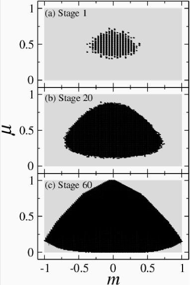
The metastable states, which correspond to $\mu=0$, are exponentially less degenerate than the states with $\mu\sim 0.5$. Since the algorithm detects the most degenerate states first, the enumeration of the metastable states becomes more and more difficult as the system size increases. However, this method represents a noticeable improvement over the exact enumeration procedure and we could study sizes up to $N=100$ (with $300$ disorder realizations).

IV.3 Simulated annealing

As introduced in Sec. III, the magnetization $m_{\alpha}(g;H,N)$ which corresponds to the maximum of $e^{Ngm}{\cal N}_{\alpha}(m;H,N)$ for a given disorder realization plays a crucial role in our analysis of the distribution of the typical metastable states in the $H$-$m$ plane. In this section, we describe a Monte Carlo procedure that yields $m_{\alpha}(g;H,N)$ without exploring the whole $(m,\mu)$ space. A similar procedure has been proposed in the context of granular materials Barrat2000 and spin systems Berg2001 .

By sampling the spin configurations with the transition probability $p(\mathbf{s}\rightarrow\mathbf{s^{\prime}})=\min\{1,\exp(Ng(m^{\prime}-m))\}$, one would obtain a distribution for the magnetizations which is proportional to $e^{gNm}\hat{\cal N}(m,\mu;H,N)$. According to the arguments of the previous section, the maximum of this distribution is dominated by the most degenerate states which correspond to $\mu>0$. This simple procedure is therefore inappropriate to analyze the statistics of the metastable states ($\mu=0$). In order to sample properly these states, one needs to introduce a bias parameter $g_{\mu}$ such that the transition from $\mathbf{s}$ to $\mathbf{s^{\prime}}$ is accepted with the probability $p(\mathbf{s}\rightarrow\mathbf{s^{\prime}})=\min\{1,\exp[N(A(m^{\prime},\mu^{\prime})-A(m,\mu))]\}$ where $A(m,g)=gm-g_{\mu}\mu$. The interesting limit for visiting the metastable states is then $g_{\mu}\rightarrow\infty$. However, since these states are much less degenerate than those with $\mu>0$, taking a large value of $g_{\mu}$ does not lead to the maximum of $e^{gNm}{\cal N}(m;H,N)$ right away. Instead, one needs to use a simulated annealing algorithm which consists in performing a sequence of MC runs, starting with $g_{\mu}=0$ and increasing slowly $g_{\mu}$ until no additional spin flip is accepted (we typically performed sequences of $2000$ MC runs, increasing $g_{\mu}$ by increments of $0.05$ up to $g_{\mu}=15$).

If ${\cal N}_{\alpha}(m;H,N)$ has a unique maximum, the magnetization resulting from this procedure is then $m_{\alpha}(g;H,N)$. In practice, however, there may be several values of $m$ for which $e^{gNm}{\cal N}_{\alpha}(m;H,N)$ is close to its maximum and the final magnetization may slightly differ from the actual $m_{\alpha}(g;H,N)$. Our simulations show that such deviations do exist but, as will be seen in Secs. V.2 and VI.2 by comparing with the analytical results for $z=2$ and the results of the other methods, they are not statistically relevant. The quenched complexity can then be obtained by considering $g$ as a function of $m$ and integrating numerically the Legendre equation $\partial\Sigma_{Q}/\partial m=-g$,

$$\Sigma_{Q}(m)=-\int_{m_{-\infty}}^{m}g(m^{\prime})dm^{\prime}$$ (18)

using the fact that $\Sigma_{Q}(m_{-\infty})=0$ since there is only one state along the hysteresis loop.

When ${\cal N}_{\alpha}(m;H,N)$ has two distinct maxima separated by a gap (see e.g. Fig. 12) so that a threshold $m_{th}$ has to be introduced in the analysis, the method does not seem to work. Indeed, we found that convergence to the metastable states (expected for $g_{\mu}\rightarrow\infty$) could not be achieved for all values of $g$. Nevertheless, it will be shown below that some useful informations can be extracted from the data even if the two branches $m^{\pm}(g;H,N)$ are not analyzed separately. With this algorithm, systems with sizes up to $N=1000$ (with $300$ disorder realizations) could then be investigated.

V Results for random graphs with $z=2$

We first present the numerical results for random graphs with connectivity $z=2$. In this case, the particular value of $\Delta$ does not introduce any qualitative change and we arbitrarily take $\Delta=2$. Our main goal is to check the validity of the numerical approaches by comparing to the analytical results of Ref. Detcheverry2005, and testing whether the different methods are consistent with each other.

V.1 Annealed complexity

Figure 5: (a) Annealed complexity $\Sigma_{A}(m;H,N)$ for $H=0$ and various system sizes (random graphs with $z=2$ and $\Delta=2$). Open symbols: exact enumeration; solid symbols: entropic sampling. The dashed line corresponds to the analytical result of Ref. Detcheverry2005, . (b) Dependence of $\Sigma_{A,\max}$ on the system size $N$. The solid line is a fit to the data. The horizontal dashed line indicates the exact value $\Sigma_{A,\max}^{\infty}=0.1$ calculated in Ref. Detcheverry2005, .(Color on line.)

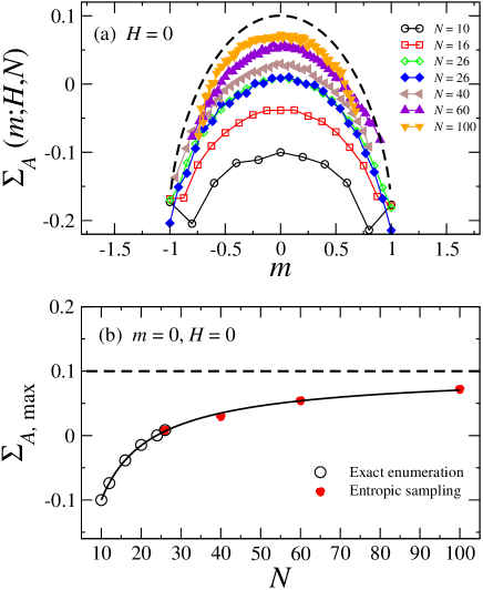
We first focus on the annealed complexity as defined by Eq. (7). Fig. 5(a) shows $\Sigma_{A}$ as a function of $m$ at $H=0$ for different sizes $N$. The data for $N\leq 26$ have been obtained by exact enumeration and those for $N\geq 26$ by entropic sampling. (Recall that the simulated annealing method is only appropriate to compute the typical quantities.) The good overlap of the two sets of data for $N=26$ shows that the two methods are consistent. At fixed $m$, the complexity increases with $N$ with a clear tendency towards the value $\Sigma_{A}^{\infty}(m;H=0)$ computed in Ref. Detcheverry2005, (dashed line in the figure). Let us analyze in more detail the case $m=0$ that corresponds to the maximum of the complexity at zero field. The size-dependence of $\Sigma_{A,\max}$ plotted in Fig. 5(b) is well described by the ansatz $\Sigma_{A,\max}=\Sigma_{A,\max}^{\infty}+aN^{-1}\ln N+bN^{-1}$ involving the three free parameters $\Sigma_{A,\max}^{\infty}$, $a$, and $b$note2 . A least-squares fit to the data yields $\Sigma_{A,\max}^{\infty}=0.10$, $a=-0.46$, $b=-0.94$, and the value of $\Sigma_{A,\max}^{\infty}$ is in remarkable agreement with the analytical result of Ref. Detcheverry2005, (actually, a fit of the data for $N\leq 26$ already provides a good estimate of $\Sigma_{A,\max}^{\infty}$). One can perform a similar analysis of the data for $m\neq 0$ but, because of the discreteness of the overall magnetization $M$, an interpolation of the curves $\Sigma_{A}(m;H,N)$ is then necessary to study the dependence with $N$ at fixed $m$.

Figure 6: (a) Annealed complexity $\Sigma_{A}(m;H,N)$ for $H=1$ and various system sizes (random graphs with $z=2$ and $\Delta=2$). The convention for symbols and lines is the same as in Fig. 5. The inset shows the size dependence of the complexity at the maximum. (b) Average magnetization $m_{A}(H)$ obtained from Eq. (19) (diamonds) and magnetization $m_{A,\max}(H,N)$ at the maximum of $\Sigma_{A}(m)$ (stars) for $N=26$. The dashed line is the analytical result of Ref. Detcheverry2005, and the dotted line represents the saturation hysteresis loop calculated in Ref. Dhar1997, .(Color on line.)

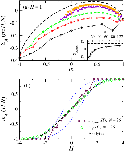
We now consider the complexity at $H=1$ (see Fig. 6(a)) to illustrate the performance of our numerical procedures in non-zero field. The curves in Fig. 6(a) are now asymmetric, with a maximum at a positive magnetization. Note that the entropic sampling method is not able to explore the whole range of magnetizations in the largest systems. Indeed, when the field $H$ is positive, the states with $m<0$ are much less degenerate than those with $m>0$, and are therefore more difficult to detect. For instance, using the value of the complexity for $N=100$, the probability of visiting a state with $m=-0.2$ is approximately 5000 times smaller than the probability of visiting the states with maximal complexity (with $m\simeq 0.42$). The detection of rare states is also limited by the number of disorder realizations investigated. This number is only $\sim 200$ for large systems, which is significantly smaller than the $5000$ realizations generated in the exact enumeration. However, we shall show below that the states which are not detected in large systems are nontypical and do not affect the quenched averages.

The numerical data for finite systems again underestimate $\Sigma_{A}^{\infty}(m,H)$ and the results must be extrapolated to $N\rightarrow\infty$. The dependence of the maximal complexity $\Sigma_{A,\max}$ with $N$ is shown in the inset of Fig. 6. The same fit as for $H=0$ yields $\Sigma_{A,\max}^{\infty}=0.079$, which is in reasonable agreement with the exact value $0.073$.

The curve $m_{A,\max}(H)$ shown in Fig. 6(b) represents the locus of the maxima of the annealed complexity in the $H$-$m$ plane. In the thermodynamic limit, the (annealed) average magnetization of the states defined for finite systems as

$$m_{A}(H,N)=\frac{\sum_{m}m\overline{{\cal N}(m;H,N)}}{\sum_{m}\overline{{\cal N}(m;H,N)}}$$ (19)

is exponentially dominated by $m_{A,\max}^{\infty}(H)$ and therefore $m_{A}^{\infty}(H)=m_{A,\max}^{\infty}(H)$. In small systems, however, $m_{A}(H,N)$ coincides with $m_{A,\max}(H,N)$ at small fields only. In particular, $m_{A,\max}(H,N)$ reaches saturation before $m_{A}(H,N)$. The deviations decrease with system size and the two curves are expected to coincide for large $N$. Interestingly, finite-size effects on $m_{A}(H,N)$ are much less important than on $m_{A,\max}(H,N)$, and $m_{A}(H,N)$ matches the analytical prediction for $m_{A}^{\infty}(H)$ even for small $N$.

V.2 Quenched complexity

Figure 7: Magnetization $m(g)$ for $H=0$ and $H=1$, and various system sizes (random graphs with $z=2$ and $\Delta=2$). Open, solid, and shaded symbols correspond to the data obtained from exact enumeration (EE), entropic sampling (ES), and simulated annealing (SA), respectively. The dashed lines represent the analytical results of Ref. Detcheverry2005, .(Color on line.)

Figure 8: (a) Quenched complexity $\Sigma_{Q}(m)$ at $H=0$ for various system sizes (random graphs with $z=2$ and $\Delta=2$). The large squares correspond to $N=1000$ and the other symbols and lines refer to the same sizes as in Fig. 5. The dashed line is the analytical result for $N\rightarrow\infty$. The inset shows the size dependence of $\Sigma_{Q,\max}$, the maximal value of the complexity. The solid line is a fit to the data. The horizontal dashed line indicates the theoretical value $\Sigma_{Q,\max}^{\infty}=0.082$ calculated in Ref. Detcheverry2005, .(Color on line.)

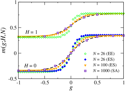
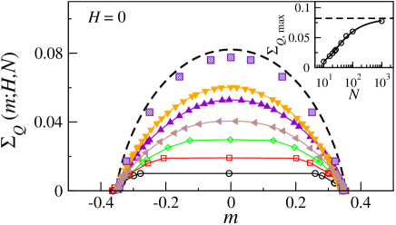
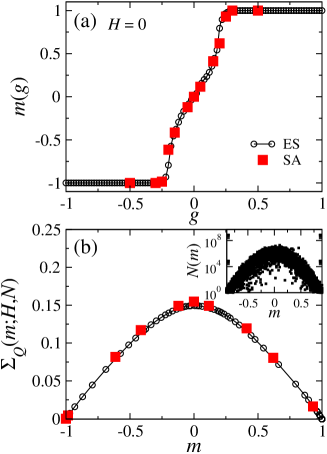
According to the analytical results of Ref. Detcheverry2005, , the quenched complexity for $z=2$ displays a single maximum as a function of $m$. Therefore, the numerical computations can be based on the definition of $\Sigma_{Q}$ given in Eq. (11). The first test is to check if the different numerical methods provide a good estimate of $m(g;H,N)$. In Fig. 7, we plot $m(g;H=0,N)$ and $m(g;H=1,N)$. For $N=26$, we compare the results obtained by exact enumeration and by entropic sampling, and the good agreement between the two curves shows that the two methods are consistent. The results for $N=1000$ only correspond to the simulated annealing method. The deviations of the data from the analytical result of Ref. Detcheverry2005, are due to finite-size effects, and the agreement becomes very good for $N=1000$. Even more important is the fact that the curves converge towards the correct limit when $g\rightarrow\pm\infty$ (actually, $m(g;H,N)$ is essentially constant when $\mid g\mid\gtrsim 1$) in spite of the lack of data for negative magnetizations in large systems (see Fig. 6(a)). Such a result confirms that (i) the states with negative $m$ which are not detected by the entropic sampling method in large systems are not typical, and (ii) the range of magnetizations for which the density of the typical states is finite (i.e., $\Sigma_{Q}>0$) is well captured by the numerical methods.

Fig. 8(a) shows the quenched complexity $\Sigma_{Q}(m)$ for $H=0$, computed from Eqs. (10) and (11), or, for $N=1000$ (with the simulated annealing method), from Eq. (18). As could be anticipated from the preceding figure, the range of magnetizations for which $\Sigma_{Q}>0$ does not depend significantly on $N$. In contrast, the values of $\Sigma_{Q}(m)$ in this interval display significant finite-size effects. As for the annealed case, the actual complexity in the thermodynamic limit is underestimated but the curves extrapolates to the correct limit. For instance, the extrapolation of the maximal complexity yields $\Sigma_{Q,\max}^{\infty}=0.082$ which is in excellent agreement with the value computed in Ref. Detcheverry2005, .

VI Results for random graphs with $z=4$

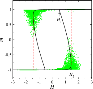
In this section devoted to random graphs with $z=4$, we shall only focus on the features of the metastable states in the low disorder regime ($\Delta<\Delta_{c}$) for which the hysteresis loop exhibits a jump discontinuity, as displayed in Fig. 9. The behavior for $\Delta>\Delta_{c}$ is indeed qualitatively similar to the one discussed above for $z=2$. Specifically, we shall take $\Delta=1$ which is smaller than the critical value $\Delta_{c}=1.78126$Dhar1997 . It has been shown that the jump in magnetization corresponds mathematically to the appearance of a new stable root in the self-consistent equation for the fixed-point probability derived in Ref. Dhar1997, . This equation has three real solutions in the range $H_{1}<H<H_{2}$ (hereafter, for simplicity, we only consider the lower branch since the upper one can be obtained by symmetry), with two of them merging and becoming complex at $H_{1}$ and $H_{2}$. As discussed in Ref. Detcheverry2005, , it is tempting to associate the reentrant curve corresponding to the “unphysical” root of the equation in the range $H_{1}<H<H_{2}$ to the limit of existence of the metastable states, i.e., to the contour $\Sigma_{Q}(m,H)=0$.

However, before discussing this issue which concerns the quenched quantities (the only ones that are actually observable), let us first summarize the results of our numerical analysis for the annealed quantities. This will provide an additional comparison with the analytical results of Ref. Detcheverry2005, .

VI.1 Annealed complexity

Figure 9: Saturation hysteresis loop on random graphs with $z=4$ and $\Delta=1$. The solid line is the curve obtained in the thermodynamic limit from the equations of Ref. Dhar1997, . The intermediate “unstable” parts (in the range $H_{1}<H<H_{2}$ for the ascending branch) are included. The hysteresis loop has a jump discontinuity at $H=\pm H_{2}$ (dashed lines). The symbols represent the loops obtained numerically in 1000 disorder realizations of size $N=100$ (for clarity, the points are not connected).(Color on line.)

Figure 10: Annealed complexity $\Sigma_{A}(m;H,N)$ for $H=0$ (a) and $H=1$ (b) and various system sizes (random graphs with $z=4$ and $\Delta=1$). The convention for symbols and lines is the same as in Fig. 5. The insets show the size dependence of the maximal complexity $\Sigma_{A,\max}$ and the corresponding fits.(Color on line.)

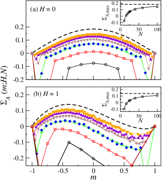
The behavior of the annealed complexity in zero field is displayed in Fig. 10(a) for different system sizes. It is similar to the one observed for $z=2$ and the function remains concave in the whole range $-1\leq m\leq 1$. Moreover, the results nicely extrapolates to the thermodynamic limit. For instance, as shown in the inset of Fig. 10(a), $\Sigma_{A,\max}$, the complexity at the maximum, extrapolates to the value $\Sigma_{A,\max}^{\infty}=0.183$ which is in excellent agreement with the theoretical value of Ref. Detcheverry2005, .

The behavior in non-zero fields is qualitatively different. In this case, the complexity is not concave in the whole range of magnetizations and two local maxima may be present. This is illustrated in Fig. 10(b) for $H=1$. In this case, the global maximum of the complexity is located at negative magnetizations although the external field is positive. This is the general behavior observed at small values of $H$. When the field is further increased, the peak at positive magnetizations (which is very close to $m=1$ for this value of $\Delta$) becomes the global maximum. As will be shown below, the quenched complexity displays a similar behavior.

The numerical results for finite systems again nicely extrapolate to the exact thermodynamic limit computed in Ref. Detcheverry2005, . The extrapolated result for $\Sigma_{A,\max}$ is $0.139$ (inset in Fig. 10(b)), which is in very good agreement with the theoretical value $\Sigma_{A,\max}^{\infty}=0.138$. One may note that the corresponding magnetization only deviates from its limiting value $m_{A,\max}^{\infty}=-0.41$ by amounts smaller than $2/N$.

VI.2 Quenched complexity

Our study of the quenched average is based on the data obtained by entropic sampling and simulated annealing on random graphs of size $N=100$ and $N=1000$. The hysteresis loops obtained in $1000$ realizations of the disorder are shown in Fig. 9 and illustrate the typical behavior of the magnetization curve in finite systems (note in particular that the average value of the field corresponding to the jump in $m$ is $H=1.72$ whereas the coercive field in the thermodynamic limit is $H=1.45$).

Let us first consider the case $H=0$. As shown in the inset of Fig. 11(b), the number of metastable states ${\cal N}(m;H=0,N)$ has a single maximum at $m\approx 0$, which implies that one can use a single Legendre transform to compute $m(g)$ and $\Sigma_{Q}(m)$ (Eqs.(8)-(11)). As can be seen in Fig. 11(a), $m(g)$ increases monotonically from $m_{-\infty}\approx-1$ to $m_{+\infty}\approx+1$ (note the good agreement between the entropic sampling and simulated annealing methods).These two values, which are extremely close (but not equal) to $\pm 1$, represent the lower and upper bounds of the magnetization of the typical states and correspond to the lower and upper branches of the hysteresis loop, respectively (one can see in Fig. 9 that these values are indeed very close to $\pm 1$). The corresponding behavior of the complexity is shown in Fig. 11(b). The curve is of course symmetric with respect to $m=0$ (one cannot see on the scale of the figure that the slope $\partial\Sigma_{Q}(m)/\partial m$ is infinite at $m=m_{\pm\infty}$).

Although the method based on two distinct Legendre transforms is neither appropriate nor necessary in this case, one may check that it yields the same results and that there is no gap in magnetization for any choice of $m_{th}$ in the interval $[m_{-\infty},m_{+\infty}]$. According to the arguments in Sec. III, this shows that the density of the typical states is strictly positive when $m_{-\infty}\leq m\leq m_{+\infty}$, that is to say inside the hysteresis loop.

Figure 11: (a) $m(g)$ and (b) $\Sigma_{Q}(m;H,N)$ for $H=0$ (random graphs with $z=4,N=100$, and $\Delta=1$). Circles and squares correspond respectively to the entropic sampling and the simulated annealing method. In (b), the inset displays the raw data for ${\cal N}(m;H=0,N)$ (obtained with the entropic sampling method) in a semi-log scale.(Color on line.)

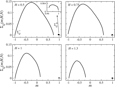
We next consider the case $H\neq 0$ and focus on the interesting region around the jump in magnetization. As can be seen in Fig. 12 that shows the raw data for ${\cal N}(m;H=1,N=100)$ obtained in $200$ samples, it is now crucial to introduce two Legendre functions $\Lambda^{-}(g)$ and $\Lambda^{+}(g)$ in order to take into account the possible existence of a gap in the magnetization of the typical states, which would imply that the curve $\Sigma_{Q}(m,H)=0$ has a reentrant part, as anticipated in Fig. 1(b). Whether or not this part of the curve is described by the “unphysical” root of the fixed-point equation of Ref. Dhar1997, (corresponding to the branch between $H_{1}$ and $H_{2}$ drawn in Fig. 9) is an independent issue which is discussed below.

Figure 12: Number of metastable states ${\cal N}(m;H=1,N)$ obtained by entropic sampling in $200$ disorder realizations (random graphs with $z=4$, $N=100$, and $\Delta=1$). Note that the right lobe is concentrated very close to $m=1$.

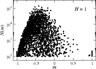
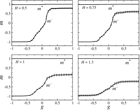
Fig. 13 summarizes the results for the magnetizations $m^{\pm}(g)$ obtained by entropic sampling. In contrast with the case $H=0$, we find that $m^{-}_{+\infty}$ is strictly smaller than $m^{+}_{-\infty}$ for the four values of $H$ considered in the figure (note that $m^{+}(g)$ is always very close to 1). This points towards the existence of a gap and two separate branches $m^{\pm}(g)$ in the thermodynamic limit. Note that these curves have been calculated with the threshold value $m_{th}=0.9$. The results do not depend on $m_{th}$, however, as long as the value is chosen in an appropriate interval whose length increases with $H$. For instance, for $H=0.5$ and $H=1.3$, the approximate intervals are $[0.85,0.95]$ and $[0.2,0.95]$, respectively. Outside these intervals one gets $m^{-}_{+\infty}=m^{+}_{-\infty}$, which simply indicates that there is a finite density of typical states with magnetization $m_{th}$.

Figure 13: Magnetizations $m^{-}(g)$ and $m^{+}(g)$ for different external fields chosen in the vicinity of the jump discontinuity (random graphs with $z=4$, $N=100$, and $\Delta=1$). The threshold in magnetization is $m_{th}=0.9$ in all cases.

The corresponding complexities $\Sigma_{Q}^{-}$ and $\Sigma_{Q}^{+}$ computed from Eqs. (III) are shown in Fig. 14. The two-peak structure resembles that of the annealed complexity in Fig. 10(b), but whereas $\Sigma_{A}$ has a minimum between the two maxima, $\Sigma_{Q}$ is not even defined in the interval $m^{-}_{+\infty}<m<m^{+}_{-\infty}$. This gap, whose size increases as $H$ approaches the coercive field, indicates that there is no typical metastable state having a magnetization in this range. (Note that $\Sigma_{Q}^{-}$ and $\Sigma_{Q}^{+}$ seem to go to zero at $m=m^{-}_{+\infty}$ and $m=m^{+}_{-\infty}$, respectively. It is possible, however, that the complexity is small but finite at these borders, in contrast with what happens for $m=m^{-}_{-\infty}$ and $m=m^{+}_{+\infty}$, i.e., along the two branches of the hysteresis loop.)

Figure 14: Quenched complexity $\Sigma_{Q}(m;H,N)$ for $H=0.5,0.75,1$ and $1.3$ (random graphs with $z=4$, $N=100$, and $\Delta=1$). The two branches correspond to $\Sigma_{Q}^{-}(m)$ and $\Sigma_{Q}^{+}(m)$, respectively. For $H=0.5$, the inset shows a magnification of $\Sigma^{+}(m)$. (The threshold in magnetization is $m_{th}=0.9$ in all cases.)

In table 1, the results for $m^{-}_{-\infty}$ and $m^{-}_{+\infty}$ are compared to the values of the magnetization obtained from the solutions of the fixed-point equation of Ref. Dhar1997, (the other branch $\Sigma_{Q}^{+}(m)$ is so close to $m=+1$ that comparing the two limits $m^{+}_{-\infty}$ and $m^{+}_{+\infty}$ with the theoretical values is not meaningful). Whereas $m^{-}_{-\infty}$ is in reasonable agreement with the theoretical value for the lower branch of the hysteresis loop, $m^{-}_{+\infty}$ significantly deviates from the solution that describes the “unstable” branch drawn in Fig. 9. This may be due, of course, to finite-size effects. In particular, the fact that our data predicts a discontinuity in the magnetization for $H=0.5$ whereas the fixed-point equation of Ref. Dhar1997, has only one root at this field is somewhat surprising. However, this may also indicate that the “unstable” branch obtained analytically does not represent the limit of existence of the metastable states in the low disorder regime. As far as we know, there is indeed no proof that the two curves should coincide.

$H$	$m_{hyst}^{-}$	$m^{-}_{-\infty}$	$m_{unst}$	$m^{-}_{+\infty}$
0.5	-0.999	$-0.995\pm 0.005$	-	$0.79\pm 0.02$
0.75	-0.998	$-0.997\pm 0.002$	$0.7$	$0.61\pm 0.04$
1	-0.994	$-0.991\pm 0.004$	$0.33$	$0.17\pm 0.05$
1.3	-0.97	$-0.96\pm 0.03$	-0.24	$-0.21\pm 0.04$

Table 1: Comparison of $m^{-}_{-\infty}(H,N)$ and $m^{-}_{+\infty}(H,N)$ with the values of the magnetization obtained from the solution of the fixed-point equation of Ref. Dhar1997, (random graphs with $z=4,N=100$ and $\Delta=1$). $m_{hyst}^{-}$ and $m_{unst}$ are the theoretical values corresponding to the ascending branch of the hysteresis loop and the “unstable” intermediate branch, respectively (for $H=0.5$, the unstable solution does not exist).

Figure 15: Magnetization $m(g)$ for $H=1$ obtained from a single Legendre transform (random graphs with $z=4$ and $\Delta=1$). Circles correspond to the entropic sampling method ($N=100$) and squares to the simulated annealing method ($N=100$: large squares, $N=1000$: small squares). The insets show the normalized distribution of $m_{\alpha}(g)$ obtained by simulated annealing for $g=0,0.05,0.15$ and $N=100$. (Color on line.)

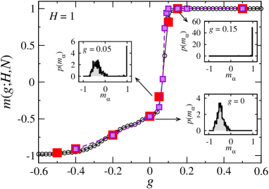
In order to study larger systems and check that the above conclusions are correct, one has to resort to the simulated annealing procedure (this is mandatory in the case of the cubic lattice, as discussed below in section VII). Unfortunately, as noted in section IV.3, this method does not work properly when one introduces a threshold $m_{th}$ so to take into account the fact that ${\cal N}(m;H,N)$ has two maxima. In consequence, we use one Legendre transform only, which has the unpleasant consequence that the two branches $m^{\pm}(g)$ are mixed. Nevertheless, as shown in Fig. 15 for $H=1$, the existence of a gap in the magnetization of the metastable states has a clear signature in $m(g)$. In order to compare with the entropic sampling method, let us first consider the case of random graphs of size $N=100$. One can see that the two methods are in perfect agreement. The comparison with the results obtained with two Legendre transforms (see Fig. 13) shows that $m(g)=m^{-}(g)$ for $g<g_{1}\simeq 0.04$ and $m(g)=m^{+}(g)$ for $g>g_{2}\simeq 0.15$. In the range $g_{1}<g<g_{2}$, the magnetization varies continuously but steeply from the branch $m^{-}(g)$ to the branch $m^{+}(g)$. This behavior comes from the fact that the distribution $p(m_{\alpha})$ of the magnetizations $m_{\alpha}(g)$ has a single peak for $g<g_{1}$ (because $\Lambda_{\alpha}^{-}(g)>\Lambda_{\alpha}^{+}(g)$ in all disorder realizations) or $g>g_{2}$ (because $\Lambda_{\alpha}^{-}(g)<\Lambda_{\alpha}^{+}(g)$), and two peaks for $g_{1}<g<g_{2}$ (because there are some realizations for which $\Lambda_{\alpha}^{-}(g)<\Lambda_{\alpha}^{+}(g)$). Therefore, in the latter case, the “mixed” quantity $m(g)$ does not represent properly the distribution of the magnetizations. However, the rapid increase of $m(g)$ signals unambiguously the passage from one branch to the other one (compare for instance with the case $z=2$ in Fig. 7). One can see that the slope becomes steeper as one goes from $N=100$ to $N=1000$, and, therefore, one expects a discontinuity in the thermodynamic limit. We stress, however, that this discontinuity has no physical meaning and that two branches $m^{\pm}(g)$ coexist from $g=-\infty$ to $+\infty$ for this value of $H$.

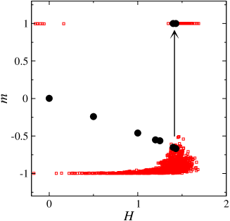
Finally, in Fig. 16, we show the curve $m(g=0;H)$ which represents the locus of the maximum of the quenched complexity in the $H-m$ plane and corresponds to the typical magnetization of the metastable states. As could be seen already in Fig. 14, the maximum for $H\lesssim 1.3$ is located at negative magnetizations despite the fact that the external field is positive. This behavior is somewhat unexpected (see the discussion in section 5 of Ref. Detcheverry2005, ) and similar to that of the (annealed) average magnetization $m_{A}(H)$ (Fig. 9 in Ref. Detcheverry2005, ). This is in contrast with the behavior observed for $z=2$ and for $z=4$ in the strong disorder regime (although the change of behavior does not exactly occur at $\Delta=\Delta_{c}$). When $H$ is further increased, the maximum of $\Sigma_{Q}^{+}$ becomes larger than the maximum of $\Sigma_{Q}^{-}$ and $m(g=0;H)$ jumps to a positive value very close to $1$ (the arrow in the figure indicates the approximate average field at which the two maxima are equal in systems of size $N=1000$). As we shall see in the following section, the qualitative behavior on the cubic lattice is quite similar.

Figure 16: Typical magnetization $m(g=0;H)$ (solid circles) of the metastable states for $H>0$ (random graphs with $z=4$, $N=1000$, and $\Delta=1$). The data are obtained by the simulated annealing method. The small squares represent the hysteresis loops obtained in $100$ disorder realizations (for clarity, the points are not connected). The case $H<0$ is obtained by symmetry. (Color on line.)

VII Results for the cubic lattice

Figure 17: Saturation hysteresis loops (small squares) for $100$ disorder realizations on a cubic lattice with $N=10^{3}$ and $\Delta=1.8$ (for clarity, the points are not connected). The solid circles represent the typical magnetization $m(g=0,H)$ for $H>0$ obtained by simulated annealing.(Color on line.)

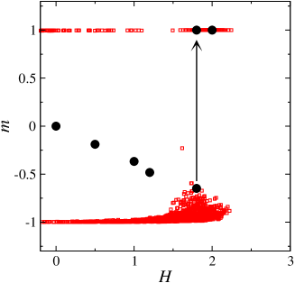
In this section, we present some results for the metastable states of the RFIM on the cubic lattice. We focus on the low disorder regime where the hysteresis loop is discontinuous. Our only objective is to show that there exists a gap in magnetization with no metastable states for a certain value of $H$ smaller than the coercive field. By continuity, this implies that there is a whole region inside the hysteresis loop where the number of states is zero. Since the entropic sampling method is limited to systems which are too small (say, $N<5\times 5\times 5$), we have used the simulated annealing algorithm and analyzed the results with a single Legendre transform, as discussed above. The system size is $N=10\times 10\times 10$ with typically 100 to 300 disorder realizations. We have chosen $\Delta=1.8$ which is smaller than the critical disorder $\Delta_{c}\simeq 2.2$ estimated in Refs.Perkovic1999 ; PerezReche2003 ).

Figure 18: Magnetization $m(g)$ for $H=1$ obtained from a single Legendre transform (simulated annealing method on a cubic lattice with $N=1000$ and $\Delta=1.8$). The insets display the normalized distribution of $m_{\alpha}$ for $g=0.05,0.08$ and $0.15$.(Color on line.)

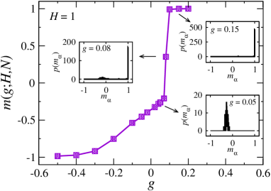
In Fig. 17, we show the hysteresis loops obtained in 100 disorder realizations. All of them display a big jump in magnetization at a coercive field whose average value is $H=1.95$. For $H=1$, the behavior of the magnetization $m(g)$ is quite similar to the one observed on random graphs for $z=4$. As shown in Fig. 18, there is a steep increase in $m(g)$ around $g\approx 0.08$ (to be contrasted with the 1d case shown in Fig. 7 or the situation for $\Delta>\Delta_{c}$), with a displacement of the peak in $p(m_{\alpha})$, the distribution of the magnetizations $m_{\alpha}(g;H,N)$, from $m\approx-0.25$ to $m\approx 1$. The interval in which two peaks are present simultaneously is very small. This suggests that there are in fact two branches $m^{\pm}(g)$, each one corresponding to a distinct branch $\Sigma^{+}(m)$ or $\Sigma^{-}(m)$ of the quenched complexity as in Fig. 14. The similarity with the scenario on random graphs is also confirmed by the behavior of $m(g=0;H)$, the typical magnetization of the metastable states. In Fig. 17, like in Fig. 16, the typical magnetization first decreases as the field increases (revealing that the maximum of the complexity occurs at negative magnetizations), and finally, at a field that is smaller than the average coercive field, jumps to a value very close to $+1$.

Note that the fact that the domain of existence of the metastable states (in the $H-m$ plane) for the cubic lattice is nonconvex is also suggested by the local mean-field calculations done in Ref. Illa2006a, in which the system is driven by the magnetization at finite temperature (see Fig. 5 in that reference).

VIII Summary and conclusions

We have studied numerically the distribution of the 1-spin-flip stable states in the RFIM at $T=0$ on random regular graphs and on the cubic lattice. Three complementary numerical methods (exact enumeration, entropic sampling, and simulated annealing) have been used to calculate the annealed and quenched complexities as a function of the magnetization and the field. The three methods have been shown to yield consistent results when applied simultaneously to the same sample. The entropic sampling algorithm allows one to study significantly larger systems than exact enumeration while obtaining interesting informations on the whole configurational spacenote3 . The simulated annealing algorithm, however, is the only one which is adapted to large systems.

In the case of random graphs, comparison with the analytical results of Ref. Detcheverry2005, (for $\Sigma_{A}(m,H)$ and $\Sigma_{Q}(m,H)$ when $z=2$ and for $\Sigma_{A}(m,H)$ when $z=4$) shows that the numerical data can be successfully extrapolated to the thermodynamic limit. In particular, for $z=4$, the concave character of $\Sigma_{A}(m)$ for $H=0$ and the non-concavity for $H\neq 0$ are well captured by the numerical results.

The present study allows us to confirm that in the low disorder regime (i.e., for $\Delta<\Delta_{c}$ on random graphs with $z=4$ or on the cubic lattice), there is a whole region inside the hysteresis loop without any typical metastable states, as illustrated in Fig. 1(b). In this case, the quenched complexity $\Sigma_{Q}(m;H)$ is positive in two distinct regions separated by a finite gap in magnetization (for $H$ close but smaller than the coercive field). The existence of the two branches is also confirmed by the discontinuous behavior of the typical magnetization of the states as a function of the field. In other words, a macroscopic discontinuity along the hysteresis loop merely indicates that there is a “hole” in the distribution of the metastable states (i.e. the domain of existence of the metastable states in the $H-m$ plane is nonconvex). It is likely that this explanation is valid for all driven systems at $T=0$ (at least when the hysteresis loop is the outer bound of all metastable states, which is the case when the coupling interactions are ferromagnetic).

Figure 19: Schematic behavior of the quenched complexity $\Sigma_{Q}(m)$ in the $\Delta$-$H$ plane for different values of $\Delta$ and $H$ in the case where a disorder-induced phase transition exists. The solid line represents the coercive field $H_{coer}(\Delta)$ at which the macroscopic discontinuity in the magnetization occurs. This line ends at the critical point (CP). Points A to D correspond to the low disorder regime ($\Delta<\Delta_{c}$) and points E and F to the strong-disorder regime ($\Delta>\Delta_{c}$). The diagram for $H<0$ is obtained by symmetry.

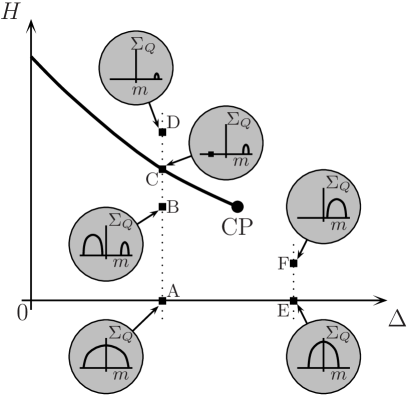
The relation between the phase diagram of the out-of-equilibrium transition in the $\Delta-H$ plane and the behavior of the quenched complexity $\Sigma_{Q}(m;H)$ as a function of $m$ is summarized schematically in Fig. 19 for different values of $H$ (for simplicity, we only consider $H>0$). The solid line represents the coercive field $H_{coer}(\Delta)$ at which the macroscopic discontinuity in the magnetization occurs. This line ends at the critical point (CP). In the strong-disorder regime (points E and F), the complexity has a single maximum that moves towards positive magnetizations as $H$ increases. This behavior is qualitatively similar to the one observed in 1 dimension (e.g., on random graphs with $z=2$). In the low disorder regime, the behavior as $H$ increases is more complicated. Whereas $\Sigma_{Q}(m)$ has a single maximum at $m=0$ when $H=0$ (point A), there are two maxima when $H$ approaches the coercive field (point B). Moreover, the global maximum is the one with the smallest magnetization, which is negative (although the field is positive). At a certain field, close to but smaller than $H_{coer}$, the maximum on the positive side of the magnetizations becomes the global one (which thus corresponds to a discontinuity in the typical magnetization of the states). At $H=H_{coer}$ (point C), all the states have a positive magnetization except one. When $H>H_{coer}$ (point D), the complexity has a single maximum at a large positive magnetization.

Note that we have not detailed the passage from one maximum to two maxima in $\Sigma_{Q}(m)$ as $H$ increases. This point is still unclear and deserves further investigation. For simplicity, we have also assumed that $\Sigma_{Q}(m)$ goes continuously to zero when $m$ approaches the borders of the gap (i.e., when $m\rightarrow m^{-}_{+\infty}$ or $m\rightarrow m^{+}_{-\infty}$, see Figs. 2 and 19). However, this is not mandatory. Note also that the behavior for larger connectivities may be more complicated than the one depicted in Fig. 19. Indeed, when $z\rightarrow\infty$, one expects to recover the mean-field behavior with its distinct $S$ shape (which in turn implies that $\Sigma_{Q}(m;H=0)$ must have three maxima when $z$ is large). This is in fact a very interesting issue which justifies an analytical study of the quenched complexity on random graphs in the large-$z$ limit. This study should also permit to understand the actual status of the “unstable” branch that can be computed from the fixed-point equation of Ref. Dhar1997, . The present numerical study seems to indicate that this branch does not coincide with the boundary $\Sigma_{Q}(m;H)=0$ but finite-size effects are too important to yield a definite conclusion.

Finally, it would be interesting (but probably highly nontrivial) to study the behavior of the quenched complexity as the critical point CP is approached. It is indeed remarkable that the essential phenomenology of the out-of-equilibrium phase transition (including the critical behavior) is encoded in $\Sigma_{Q}(m,H$).

IX Acknowledgements

We acknowledge fruitful discussions with L. Truskinovsky and E. Vives. FJPR was supported by the Marie-Curie contract MRTN-CT-2004-505226 and by the spanish grant MEC EX2005-0792. The LPTMC is the UMR 7600 of the CNRS.

References

- (1) J. P. Sethna, K. A. Dahmen, and O. Perković in The Science of Hysteresis II, edited by G. Bertotti and I. Mayergoyz, Academic Press, Amsterdam (2006).
- (2) F. Detcheverry, M.L. Rosinberg, and G. Tarjus, Eur. Phys. J. B 44, 327 (2005).
- (3) J. P. Sethna, K. A. Dahmen, S. Kartha, J. A. Krumhansl, B. W. Roberts, and J. D. Shore, Phys. Rev. Lett. 70, 3347 (1993).
- (4) X. Illa, M. L. Rosinberg, and E. Vives, Phys. Rev. B 74, 224403 (2006).
- (5) X. Illa, M. L. Rosinberg, P. Shukla, and E. Vives, Phys. Rev. B 74, 224404 (2006).
- (6) M. Mezard and G. Parisi, Eur. Phys. J. B 20, 217 (2001). (1993).
- (7) D. Dhar, P. Shukla, and J. P. Sethna, J. Phys. A: Math. Gen. 30, 5259 (1997).
- (8) O. Perković, K. A. Dahmen, and J. P. Sethna, Phys. Rev. B 59, 6106 (1999).
- (9) F. J. Perez-Reche and E. Vives, Phys. Rev. B 67, 134421 (2003); ibid 70, 214422 (2004).
- (10) F. Colaiori, M. J. Alava, G. Durin, A. Magni, and S. Zapperi, Phys. Rev. Lett. 92, 257203 (2004).
- (11) C. M. Newman and D. L. Stein, Phys. Rev. E 60, 5244 (1999). For instance, the 2-spin-flip dynamics has been recently analyzed by E. Vives, M. L. Rosinberg, and G. Tarjus, Phys. Rev. B 71, 134424 (2005).
- (12) R. Cherrier, D. S. Dean, and A. Lefèvre, J. Phys. A: Math. Gen. 36, 3955 (2003).
- (13) if . The ferromagnetic interaction ensures that this order relation is preserved by the dynamics during a monotonous field history (i.e., if increases from to , then ). This is the so-called no-passing ruleSethna1993 .
- (14) J. Lee, Phys. Rev. Lett. 71, 211 (1993).
- (15) I. Shteto, J. Linares, and F. Varret, Phys. Rev. E 56, 5128 (1997).
- (16) B. A. Berg and T. Neuhaus, Phys. Rev. Lett. 68, 9 (1992).
- (17) A. Barrat, J. Kurchan, V. Loreto, and M. Sellitto, Phys. Rev. E 63, 051301 (2001).
- (18) J. Berg and M. Sellitto, Phys. Rev. E. 65, 016115 (2001).
- (19) The behavior of in the thermodynamic limit is expected to be dominated by the exponential . Accordingly, for finite systems, we assume that , introducing the natural subdominant dependencies associated with an exponential behavior. The ansatz for is readily obtained by using this expression in Eq. (7).
- (20) For instance, one can compute the quenched complexity associated to configurations that are not fully metastable (i.e., with a “misalignment“ parameter ). Interestingly, we have found that the gap in magnetization also concerns the states with sufficiently small. We plan to come back to this issue in a future work.