Density Functional Theory of Inhomogeneous Liquids: I. The liquid-vapor interface in Lennard-Jones fluids.

Abstract

A simple model is proposed for the direct correlation function (DCF) for simple fluids consisting of a hard-core contribution, a simple parametrized core correction and a mean-field tail. The model requires as input only the free energy of the homogeneous fluid, obtained e.g. from thermodynamic perturbation theory. Comparisons to the DCF obtained from simulation of a Lennard-Jones fluid shows this to be a surprisingly good approximation for a wide range of densities. The model is used to construct a density functional theory for inhomogeneous fluids which is applied to the problem of calculating the surface tension of the liquid-vapor interface. The numerical values found are in good agreement with simulation.

I Introduction

The modern understanding of liquid-vapor interfaces begins with the seminal paper of van der Waals in which he introduces what is now known as the square-gradient approximation to the free energy of inhomogeneous systems and the mean-field approximationvan der Waals (1894); Rowlinson (1979). That work was developed from a thermodynamic perspective which has been superseded by more fundamental, statistical mechanical approachesEvans (1979); Rowlinson and Widom (2002); Lutsko (2006). In the modern approach, it is possible to give formally exact expressions for the free energy in terms of structural quantities such as the pair-distribution function and the direct correlation function. In practice, these expressions must be approximated leading to a compromise between the two goals of simplicity and accuracy. Given modern computational resources, simplicity is not an overriding constraint when dealing with simple fluids governed by spherically symmetric pair potentials but it quickly does become an issue for more complex systems such as solids, fluids governed by anisotropic potentials, extended molecules, etc. When confronted with these types of complications, there is often little choice than to revert to the most primitive mean field models and to hope that the qualitative picture obtained is sufficient. The object of the present work is to present an approach which is little more complex than the simplest mean field theory and yet which gives quantitatively accurate results.

The original theory of van der Waals was based on two basic approximations. First is what in modern language would be called a mean-field approximation whereby the microscopic structure of the liquid is neglected and the only spatial variation taken into consideration is a continuous variation of the density. This means that the interaction energy for a system of molecules interacting via a pair potential can be expressed in the form

$$\int_{V}\int_{V}\rho\left(\mathbf{r}_{1}\right)\rho\left(\mathbf{r}_{2}\right)v\left(\mathbf{r}_{12}\right)d\mathbf{r}_{1}d\mathbf{r}_{2}$$ (1)

where $V$ is the volume of the system, $\rho\left(\mathbf{r}\right)$ is the local density and $v\left(\mathbf{r}_{12}\right)$ is the pair potential. The second is a gradient expansion about the center of mass. This model was also discussed by Cahn and HilliardCahn and Hilliard (1958). Today, there are two more or less fundamental approaches to the description of inhomogeneous liquidsEvans (1979); Rowlinson and Widom (2002). The oldest are the integral equation methods where the object is to solve the Ornstein-Zernike equation, which relates the pair-distribution function to the direct correlation function, subject to an independent closure condition. This approach is one of the most reliable methods for calculating the properties of simple fluids. It is however intrinsically somewhat complex since the fundamental objects being determined, e.g. the pair distribution function, are two-body functions. The main alternative are density functional theories which are somewhat simpler since the local density is a one-point function. The utility of DFT for the description of liquid-vapor interfaces was first demonstrated by the work of Ebner, Saam and StroudEbner et al. (1976). They used an approximate DFT which was, as they themselves later wroteSaam and Ebner (1977). somewhat ad hoc. The key quantity needed to evaluate the theory was the direct correlation function (DCF) of the homogeneous fluid which was obtained from the Percus-Yevick integral theory. However, for interfacial calculations, the DCF was needed for all densities from that of the liquid to that of the vapor which is problematic as the integral theory does not possess solutions in the two-phase region. Ebner et al. were therefore forced to interpolate the DCF’s from the region where the integral equation could be solved through the region without a solution. The resulting values for the surface tension of a Lennard-Jones fluid were in fact quite reasonable.

Since this early work, the DFT approach to interfacial problems has developed primarily along two different lines. One is based on the perturbative expression for the free energy in terms of a hard-sphere contribution and a perturbative correction involving the potential and the direct correlation function of hard spheres( see e.g. Tang et al. (1991); Wadewitz and Winkelmann (2000)). This approach has the advantage that it reduces to the rather accurate perturbative expression for the free energy for the homogeneous fluids and therefore gives a good description of the phase diagram. Indeed, as discussed by Wadewitz and Winkelmann (2000), this is one of the main motivations for using this model. The second approach is more in line with the work of Ebner et al and is based on the direct correlation function (DCF) and the exact relations between the DCF and the free energy. A good example is the recent work of Tang and coworkersTang and Wu (2003, 2004); Tang (2005) who approximate the DCF by that obtained from an approximate solution of the mean-spherical approximation. (In the mean spherical approximation, the Ornstein-Zernike equation is solved by assuming that there is an effective hard core inside of which the pair distribution function vanishes and outside of which the DCF is equal to $-\beta v\left(\mathbf{r}_{12}\right)$). To further simplify, Tang approximates the Lennard-Jones interaction by a sum of Yukawa potentials so that the resulting mean-spherical model can be solved analytically both exactlyHoye and Blum (1977) and within the first order approximationTang (2003). This is then used in an approximate DFT, somewhat different from that of Ebner et al, to calculate a variety of properties of inhomogeneous Lennard-Jones fluids including the surface tension of the liquid-vapor interfaceTang (2005) and the structure of confined fluidsTang and Wu (2004),Tang (2004). Since surface tension in particular is well-known to be very sensitive to the range of the potential, the Yukawa’s, which are short-ranged, must eventually be replaced by the original potential in order to account for the long-ranged contributions to the surface tension.

The perturbation-theory approach requires as input the pair-distribution function of the reference system, usually hard-spheres for simple fluids. Even when the reference fluid is hard-spheres, the pair-distribution function is not an easy object to work with (see ref.Wadewitz and Winkelmann (2000)) and the calculations would be even more difficult for more complex interactions. On the other hand, the difficulty with the DCF-based theories is that there have been few options for getting the DCF required in the theories: either the mean-field approximation such as eq.(1) above is used (which is very crude) or the full machinery of liquid-state theory is used (which is expensive). However, given that even when the latter approach is used, quite ad hoc corrections, such as the interpolation of Ebner et al., are needed suggests that the effort expended to try to produce as good a DCF as possible is perhaps unnecessary. Instead, the work of Tang et al suggests that the most important ingredient beyond the mean-field form is that the underlying equation of state should be reasonably accurate. The present work aims to test this intuition by studying a minimal extension of the mean-field model for the DCF designed so as to reproduce a known equation of state. Specifically, the model proposed here consists of a hard core, described by the Fundamental Measure DFTRosenfeld (1989); Rosenfeld et al. (1990); Tarazona (2000); Roth et al. (2002), a mean-field type tail and a simple polynomial correction within the core with parameters chosen to give the desired equation of state. The utility of the model lies in the fact that the equation of state of the homogeneous bulk fluid, is much easier to determine than are structural properties such as the DCF and the pair distribution function and it is much less sensitive to the details of the interaction potential. In this work, for application to the Lennard-Jones fluid, first order thermodynamic perturbation theory is used. This approach represents a relatively minimal extension of the mean field model and as shown below, even a relatively crude model gives good results for the surface tension of the liquid-vapor interface. It is in keeping with the idea that the DCF should be a relatively simple object as illustrated, e.g., by the contrast in hard-spheres as described by the Percus-Yevick approximation where the pair-distribution function is a complicated function with a lot of structure whereas the DCF is just a cubic polynomial within the hard core. The same is true in the analytic solution of the mean-spherical approximation for a sum of YukawasHoye and Blum (1977).

In the next Section, the basic elements of Density Functional Theory are reviewed. A plausible, but uncontrolled, approximation is introduced to give a framework suitable for practical applications. It is shown that further approximations give the functional used by Ebner et al.Ebner et al. (1976) as well as that introduced by TangTang (2005) . Because it is still often discussed in the literature, see e.g. refs. Cornelisse et al. (1997) and Duque et al. (2004), the square-gradient approximation is also described. The third Section discusses the extended mean-field approximation for the DCF. Different versions are described depending on how accurately the tail of the DCF is modeled. These are compared to the simulation data of Llano-Restrepo and ChapmanLlano-Restrepo and Chapman (1992) and it is demonstrated that these models are in good agreement with the simulations. In the fourth Section, the calculation of the surface tension for the liquid-vapor interface of the Lennard-Jones fluid are presented. Aside from testing the model for the DCF, the results from the different approximate DFTs are compared and it is found that they are all in reasonable agreement with one another and with the results from simulation. The paper ends with a discussion of the results.

II Theory

II.1 Density Functional Theory formalism

Density Functional Theory is based on the fact that there is a one-to-one correspondence between applied external fields, $V_{ext}\left(\mathbf{r}\right)$, and the ensemble-averaged equilibrium density profile, $\rho\left(\mathbf{r}\right)$. For a given external field, there is a functional of the form

$$\Omega\left[n,V_{ext}\right]=F\left[n\right]-\int\mu n\left(\mathbf{r}\right)d\mathbf{r}+\int V_{ext}\left(\mathbf{r}\right)n\left(\mathbf{r}\right)dr$$ (2)

such that $\Omega\left[n,V_{ext}\right]$ is extremized by the equilibrium density profile giving

$$0=\left.\frac{\delta\Omega\left[n,V_{ext}\right]}{\delta n\left(\mathbf{r}\right)}\right|_{n\left(\mathbf{r}\right)=\rho\left(\mathbf{r}\right)}=\left.\frac{\delta F\left[n\right]}{\delta n\left(\mathbf{r}\right)}\right|_{n\left(\mathbf{r}\right)=\rho\left(\mathbf{r}\right)}-\mu+V_{ext}\left(\mathbf{r}\right).$$ (3)

Throughout this Section, square brackets are used to denote a functional dependence and round brackets to denote an ordinary function. In general, the domain of the spatial integrals is unbounded with the effect of any walls being explicitly accounted for by the external field. The presence of a hard wall will, in this way, manifest itself by the equilibrium density profile obtained from eq.(3) giving zero density outside the wall. However, for clarity, a volume $V$ will be explicitly indicated below with the understanding that it simply connotes the region of non-zero density. The functional $F$ is conveniently written as a sum of an ideal gas contribution,

$$\beta F_{id}\left[n\right]=\int_{V\ }\left(n\left(\mathbf{r}\right)\log\left(\Lambda^{3}n\left(\mathbf{r}\right)\right)-n\left(\mathbf{r}\right)\right)d\mathbf{r,}$$ (4)

where $\Lambda$ is the thermal wavelength, and a remaining, excess contribution $F_{ex}\left[n\right].$ In general, the latter is unknown, but since it depends only on the density, and not explicitly on the field, it can be expressed by expansion about a uniform state having constant density $\overline{\rho}_{0}$ as

$$\frac{1}{V}\beta F_{ex}\left[n\right] = \frac{1}{V}\beta F_{ex}\left(\overline{\rho}_{0}\right)+\beta\mu_{ex}\left(\overline{\rho}_{0}\right)\left(\overline{n}-\overline{\rho}_{0}\right)$$

$$-\frac{1}{V}\sum_{j=2}^{\infty}\frac{1}{j!}\int_{V}...\int_{V}\left(n\left(\mathbf{r}_{1}\right)-\overline{\rho}_{0}\right)...\left(n\left(\mathbf{r}_{j}\right)-\overline{\rho}_{0}\right)c_{j}\left(\mathbf{r}_{1},...,\mathbf{r}_{j};\overline{\rho}_{0}\right)d\mathbf{r}_{1}...d\mathbf{r}_{j}$$

where $\mu_{ex}\left(\overline{\rho}_{0}\right)=\frac{\partial}{\partial\overline{\rho}_{0}}\frac{1}{V}F_{ex}\left(\overline{\rho}_{0}\right)$ and where $c_{j}\left(\mathbf{r}_{1},...,\mathbf{r}_{j};\overline{\rho}_{0}\right)$ is the j-body direct correlation function of a uniform fluid. These are simply the functional derivatives of the $F_{ex}\left[n\right]$ in the uniform limit,

$$c_{j}\left(\mathbf{r}_{1},...,\mathbf{r}_{j};\overline{\rho}_{0}\right)=\lim_{n\left(\mathbf{r}\right)\rightarrow\overline{\rho}_{0}}c_{j}\left(\mathbf{r}_{1},...,\mathbf{r}_{j};\left[n\right]\right)=-\lim_{n\left(\mathbf{r}\right)\rightarrow\overline{\rho}_{0}}\frac{\delta^{j}\beta F_{ex}\left[n,V_{ext}\right]}{\delta n\left(\mathbf{r}_{1}\right)...\delta n\left(\mathbf{r}_{j}\right)}$$ (6)

and it can be shown that they correspond to the usual direct correlation functions discussed in liquid state theoryEvans (1979). Thus, the free energy functional of an arbitrary non-uniform system is expressed in terms of the properties of a uniform fluid. This series can be resummed to give

$$\beta F_{ex}\left[n\right] = \beta F_{ex}\left(\overline{\rho}_{0}\right)+V\beta\mu_{ex}\left(\overline{\rho}_{0}\right)\left(\overline{n}-\overline{\rho}_{0}\right)$$

$$-\int_{V}d\mathbf{r}_{1}\int_{V}d\mathbf{r}_{2}\int_{0}^{1}d\lambda\int_{0}^{\lambda}d\lambda^{\prime}\left(n\left(\mathbf{r}_{1}\right)-\overline{\rho}_{0}\right)\left(n\left(\mathbf{r}_{2}\right)-\overline{\rho}_{0}\right)c_{2}\left(\mathbf{r}_{1},\mathbf{r}_{2};\left[n_{\lambda^{\prime}}\right]\right)$$

where $n_{\lambda}\left(\mathbf{r}\right)=\overline{\rho}_{0}+\lambda\left(n\left(\mathbf{r}\right)-\overline{\rho}_{0}\right)$ the integral depends on the two-body direct correlation function for an arbitrary density profile. In particular, in the case of a uniform density $n(\mathbf{r})=\overline{n}$ the last term on the right gives the standard result for homogeneous fluids,

$$\frac{1}{V}\beta F_{ex}\left(\overline{n}\right)=\frac{1}{V}\beta F_{ex}\left(\overline{\rho}_{0}\right)+\beta\mu_{ex}\left(\overline{\rho}_{0}\right)\left(\overline{n}-\overline{\rho}_{0}\right)-\int_{V}\int_{0}^{1}\left(\overline{n}-\overline{\rho}_{0}\right)^{2}c_{2}\left(r_{12};\overline{\rho}_{0}+\lambda\left(\overline{n}-\overline{\rho}_{0}\right)\right)\left(1-\lambda\right)d\lambda d\mathbf{r}_{12},$$ (8)

which relates the DCF of the homogeneous system to the thermodynamics. (Note that in writing this equation, the fact that the DCF of a simple fluid depends only on the scalar $r_{12}=\left|\mathbf{r}_{1}-\mathbf{r}_{2}\right|$ has been explicitly indicated.) An important point in all of these exact expressions is that the results for the free energy of the system with density $n\left(\mathbf{r}\right)$ (or the liquid with density $\overline{n}$) are independent of the choice of reference liquid density $\overline{\rho}_{0}$. This is of course not true when approximations are introduced but any approximation will involve implicitly or explicitly a choice of reference density. In this Section, the reference state has been explicitly indicated so as to make this clear.

While the n-body DCFs for a uniform system are in principle accessible, in practice only quantities up to the two-body direct correlation function are known with any confidence for arbitrary pair potentials using liquid state theory such as the integral equations of Rogers and YoungRogers and Young (1984) and of Hansen and ZerahZerah and Hansen (1986). Even then, the integral equations only possess solutions for certain ranges of density and temperature. Furthermore, if the goal is to develop a theory which can eventually be applied to more complex systems involving asymmetric interactions or the solid phase, then this approach is infeasible.

II.2 Approximations to the exact theory

In order to construct a more practical approach, it is first noted that the only system for which good general approximations to the functional $F_{ex}\left[n\right]$ exist is that of hard spheres. It is therefore useful to consider the difference

$$\beta F_{ex}\left[n\right] = \beta F_{ex}^{HS}\left[n\right]+\beta\Delta F_{ex}\left(\overline{\rho}_{0};d\right)+V\beta\Delta\mu_{ex}\left(\overline{\rho}_{0};d\right)\left(\overline{n}-\overline{\rho}_{0}\right)$$

$$-\sum_{j=2}^{\infty}\frac{1}{j!}\int_{V}...\int_{V}\left(n\left(\mathbf{r}_{1}\right)-\overline{\rho}_{0}\right)...\left(n\left(\mathbf{r}_{j}\right)-\overline{\rho}_{0}\right)\Delta c_{j}\left(\mathbf{r}_{1},...,\mathbf{r}_{j};\overline{\rho}_{0}\right)d\mathbf{r}_{1}...d\mathbf{r}_{j}$$

$$= \beta F_{ex}^{HS}\left[n\right]+\beta\Delta F_{ex}\left(\overline{\rho}_{0};d\right)+V\beta\Delta\mu_{ex}\left(\overline{\rho}_{0};d\right)\left(\overline{n}-\overline{\rho}_{0}\right)$$

$$-\int_{V}d\mathbf{r}_{1}\int_{V}d\mathbf{r}_{2}\int_{0}^{1}d\lambda\int_{0}^{\lambda}d\lambda^{\prime}\left(n\left(\mathbf{r}_{1}\right)-\overline{\rho}_{0}\right)\left(n\left(\mathbf{r}_{2}\right)-\overline{\rho}_{0}\right)\Delta c_{2}\left(\mathbf{r}_{1},\mathbf{r}_{2};\left[n_{\lambda^{\prime}}\right]\right)$$

where $\Delta c_{j}\left(\mathbf{r}_{1},...,\mathbf{r}_{j};\overline{\rho}_{0}\right)=c_{j}\left(\mathbf{r}_{1},...,\mathbf{r}_{j};\overline{\rho}_{0}\right)-c_{j}^{HS}\left(\mathbf{r}_{1},...,\mathbf{r}_{j};\overline{\rho}_{0};d\right)$, etc. Then, the simplest nontrivial approximation is to truncate the infinite series after the first term giving the theory studied by RosenfeldRosenfeld (1993),

$$\beta F_{ex}\left[n\right] \simeq \beta F_{ex}^{HS}\left[n\right]+\beta\Delta F_{ex}\left(\overline{\rho}_{0};d\right)+V\beta\Delta\mu_{ex}\left(\overline{\rho}_{0};d\right)\left(\overline{n}-\overline{\rho}_{0}\right)$$

$$-\frac{1}{2}\int_{V}\int_{V}\left(n\left(\mathbf{r}_{1}\right)-\overline{\rho}_{0}\right)\left(n\left(\mathbf{r}_{2}\right)-\overline{\rho}_{0}\right)\Delta c_{2}\left(r_{12};\overline{\rho}_{0}\right)d\mathbf{r}_{1}d\mathbf{r}_{2}.$$

However, while this is suitable for some applications, it suffers from the fact that the results depend on the choice of reference density, $\overline{\rho}_{0}$. In fact, in the uniform limit, it will not give the correct free energy for the bulk fluid unless one demands that $\overline{\rho}_{0}=\overline{n}$. This also works for some inhomogeneous systems such as a fluid in contact with a wall since there is a unique bulk limit far from the wallTang and Wu (2004). However, in other problems, most notably that of the planar liquid-vapor interface, there is no unique bulk limit and no choice of reference density gives the correct bulk free energy in all bulk regionsTang (2005).

Perhaps the most natural approximation that is exact in the limit of a homogeneous liquid is to replace the exact DCF for the inhomogeneous system by the DCF of a homogeneous system evaluated at some position-dependent density. There is considerable ambiguity in how to do this since the DCF is a two-point function and the density is a one-point function. The only formal requirements are that the DCF must be symmetric in its arguments and it must reduce to the known result in the uniform limit. Perhaps the two simplest approximations satisfying both requirements are

$$\Delta c_{2}\left(\mathbf{r}_{1},\mathbf{r}_{2};\left[n\right]\right)\simeq\Delta c_{2}\left(r_{12};\frac{n\left(\mathbf{r}_{1}\right)+n\left(\mathbf{r}_{2}\right)}{2}\right)$$ (11)

and

$$\Delta c_{2}\left(\mathbf{r}_{1},\mathbf{r}_{2};\left[n\right]\right)\simeq\frac{1}{2}\left(\Delta c_{2}\left(r_{12};n\left(\mathbf{r}_{1}\right)\right)+\Delta c_{2}\left(r_{12};n\left(\mathbf{r}_{2}\right)\right)\right).$$ (12)

In the following, these will be referred to as the local DCF approximations (LDCF-I and LDCF-II, respectively).

When the LDCF-I approximation is substituted into eq. (II.2), one obtains after some rearrangement,

$$\beta F_{ex}\left[n\right]=\beta F_{ex}^{HS}\left[n\right]+\int d\mathbf{r}\;\beta\Delta f\left(n\left(\mathbf{r}\right)\right)$$ (13)

$$+\frac{1}{4}\int_{V}d\mathbf{r}_{1}\int_{V}d\mathbf{r}_{2}\left(n\left(\mathbf{r}_{1}\right)-n\left(\mathbf{r}_{2}\right)\right)^{2}\Delta\overline{\overline{c}}_{2}\left(r_{12};\frac{n\left(\mathbf{r}_{1}\right)+n\left(\mathbf{r}_{2}\right)}{2},\overline{\rho}_{0}\right)$$

$$-\frac{1}{2}\int_{V}d\mathbf{r}_{1}\int_{V}d\mathbf{r}_{2}\left[\begin{array}[]{c}\left(\frac{n\left(\mathbf{r}_{1}\right)+n\left(\mathbf{r}_{2}\right)}{2}-\overline{\rho}_{0}\right)^{2}\Delta\overline{\overline{c}}_{2}\left(r_{12};\frac{n\left(\mathbf{r}_{1}\right)+n\left(\mathbf{r}_{2}\right)}{2},\overline{\rho}_{0}\right)\\ -\left(n\left(\mathbf{r}_{1}\right)-\overline{\rho}_{0}\right)^{2}\Delta\overline{\overline{c}}_{2}\left(r_{12};n\left(\mathbf{r}_{1}\right),\overline{\rho}_{0}\right)\end{array}\right]$$ (16)

where $\Delta f\left(n\right)=\frac{1}{V}\beta F_{ex}\left(n\right)-\frac{1}{V}\beta F_{ex}^{HS}\left(n\right)$ is the difference in free energy per unit volume of the homogeneous liquid at density $n$ and the density of a homogeneous hard-sphere liquid at the same density and where

$$\Delta\overline{\overline{c}}_{2}\left(r;n,\overline{\rho}_{0}\right)\equiv 2\int_{0}^{1}\int_{0}^{\lambda}\Delta c_{2}\left(r;\overline{\rho}_{0}+\lambda^{\prime}\left(n-\overline{\rho}_{0}\right)\right)d\lambda^{\prime}d\lambda.$$ (17)

The LDCF-II gives a somewhat simpler expression,

$$\beta F_{ex}\left[n\right] = \beta F_{ex}^{HS}\left[n\right]+\int d\mathbf{r}\;\Delta f\left(n\left(\mathbf{r}\right)\right)$$

$$+\frac{1}{2}\int_{V}\int_{V}\left(n\left(\mathbf{r}_{1}\right)-\overline{\rho}_{0}\right)\left(n\left(\mathbf{r}_{1}\right)-n\left(\mathbf{r}_{2}\right)\right)\Delta\overline{\overline{c}}_{2}\left(r_{12};n\left(\mathbf{r}_{1}\right),\overline{\rho}_{0}\right)d\mathbf{r}_{2}d\mathbf{r}_{1}.$$

This has the intuitively appealing form of the sum of a hard-sphere contribution, a local free energy approximation and a nonlocal term that explicitly depends, via the factor $\left(n\left(\mathbf{r}_{1}\right)-n\left(\mathbf{r}_{2}\right)\right)$ , on the inhomogeneity of the fluid. To make contact with earlier work, and anticipating the model for the DCF discussed below, assume that the DCF can be written as the sum of a short-ranged part, $\Delta\overline{\overline{c}}_{2}^{core}\left(r_{12};n\left(\mathbf{r}_{1}\right),\overline{\rho}_{0}\right)$, and a density-independent tail, $\Delta\overline{\overline{c}}_{2}^{tail}\left(r_{12}\right)$. Then, the excess free energy can be written as

$$\beta F_{ex}\left[n\right] = \beta F_{ex}^{HS}\left[n\right]+\int d\mathbf{r}\;\Delta f\left(n\left(\mathbf{r}\right)\right)$$

$$+\frac{1}{4}\int_{V}\int_{V}\left(n\left(\mathbf{r}_{1}\right)-n\left(\mathbf{r}_{2}\right)\right)^{2}\Delta c_{2}^{tail}\left(r_{12}\right)d\mathbf{r}_{2}d\mathbf{r}_{1}$$

$$+\frac{1}{2}\int_{V}\int_{V}\left(n\left(\mathbf{r}_{1}\right)-\overline{\rho}_{0}\right)\left(n\left(\mathbf{r}_{1}\right)-n\left(\mathbf{r}_{2}\right)\right)\Delta\overline{\overline{c}}_{2}^{core}\left(r_{12};n\left(\mathbf{r}_{1}\right),\overline{\rho}_{0}\right)d\mathbf{r}_{2}d\mathbf{r}_{1}$$

Since the core contribution is assumed to be short ranged, is makes sense to expand in terms of the difference $\left(n\left(\mathbf{r}_{1}\right)-n\left(\mathbf{r}_{2}\right)\right)$ giving, see Appendix A for details,

$$\beta F_{ex}\left[n\right] = \beta F_{ex}^{HS}\left[n\right]+\int d\mathbf{r}\;\Delta f\left(n\left(\mathbf{r}\right)\right)$$

$$+\frac{1}{4}\int_{V}\int_{V}\left(n\left(\mathbf{r}_{1}\right)-n\left(\mathbf{r}_{2}\right)\right)^{2}\left[2\int_{0}^{1}\lambda\Delta c_{2}\left(r_{12};\overline{\rho}_{0}+\lambda\left(\frac{n\left(\mathbf{r}_{1}\right)+n\left(\mathbf{r}_{2}\right)}{2}-\overline{\rho}_{0}\right)\right)d\lambda\right]d\mathbf{r}_{1}d\mathbf{r}_{2}$$

$$+...$$

where the neglected terms are integrals involving $\left(n\left(\mathbf{r}_{1}\right)-n\left(\mathbf{r}_{2}\right)\right)^{n}$ for $n>2$. Expanding $\Delta c_{2}$ about $\lambda=1$ , gives to leading order

$$\beta F_{ex}\left[n\right] = \beta F_{ex}^{HS}\left[n\right]+\int d\mathbf{r}\;\Delta f\left(n\left(\mathbf{r}\right)\right)$$

$$+\frac{1}{4}\int_{V}\int_{V}\left(n\left(\mathbf{r}_{1}\right)-n\left(\mathbf{r}_{2}\right)\right)^{2}\Delta c_{2}\left(r_{12};\frac{n\left(\mathbf{r}_{1}\right)+n\left(\mathbf{r}_{2}\right)}{2}\right)d\mathbf{r}_{1}d\mathbf{r}_{2}$$

$$+...$$

which resembles the well-known theory of Ebner et al.Ebner et al. (1976); Saam and Ebner (1977). (In the original work, the hard-sphere contribution was not treated separately. However, because the approximation scheme used here for the excess part is the same, this will be referred to as the ESS theory after the authors of the first paper.) If instead one expands $\Delta c_{2}$ about $\lambda=0$ and keeps only the leading term, the result is

$$\beta F_{ex}\left[n\right] = \beta F_{ex}^{HS}\left[n\right]+\int d\mathbf{r}\;\beta\Delta f\left(n\left(\mathbf{r}\right)\right)$$

$$+\frac{1}{4}\int_{V}\int_{V}\left(n\left(\mathbf{r}_{1}\right)-n\left(\mathbf{r}_{2}\right)\right)^{2}\Delta c_{2}\left(r_{12};\overline{\rho}_{0}\right)d\mathbf{r}_{1}d\mathbf{r}_{2}$$

$$+...$$

which is the recent theory of TangTang (2005).

Finally, having outlined the approximations that will be used in the applications below, it is worth noting some formal differences between them. The LDCF approximations involve a minimal conceptual element, eq.(11) or eq.(12), but as anticipated above and as shown explicitly below, the resulting free energy is no longer independent of the chosen reference state. For the liquid-vapor interface, it will turn out that the dependence on $\overline{\rho}_{0}$ is quite weak except that if it is chosen too large, no stable profile is found. For at least this application, these theories are practically, if not formally, unique. The same is true of the Tang theory although the dependence on the reference state is found to be somewhat stronger than for the LDCF theories. The ESS theory is independent of the reference state. However, hidden in its derivation is an expansion of the density integrals in eq.(II.2) about an arbitrarily chosen point ($\lambda=1$). Perhaps it could be argued that the expansion about $\lambda=1$ is justified by the fact that it makes the theory independent of the reference state, but whether or not this is convincing seems to be a matter of taste.

II.3 Square-gradient approximation

Another approach to the description of inhomogeneous systems is the square-gradient approximationvan der Waals (1894); Rowlinson (1979); Rowlinson and Widom (2002); Lutsko (2006). If the density varies sufficiently slowly, it is possible to expand the density-dependence of the exact free energy functional so as to obtain

$$\beta F_{ex}\left[n\right]=\int_{V}\;\left[\beta f\left(n\left(\mathbf{r}\right)\right)+\frac{1}{2}g\left(n\left(\mathbf{r}\right)\right)\left(\mathbf{\nabla}n\left(\mathbf{r}\right)\right)^{2}+...\right]d\mathbf{r}$$ (23)

where the neglected terms involve higher order derivatives. The coefficient of the gradient term is

$$g\left(n\right)=\frac{1}{6}\int_{V}r^{2}c_{2}\left(r;n\right)d\mathbf{r}$$ (24)

showing that the square-gradient approximation is another way to use information about the uniform system to construct a description of nonuniform systems. The density profile is determined by the Euler-Lagrange equation

$$\mathbf{\nabla}\cdot\left(g\left(n\left(\mathbf{r}\right)\right)\mathbf{\nabla}n\left(\mathbf{r}\right)\right)-\frac{\partial g\left(n\left(\mathbf{r}\right)\right)}{\partial n\left(\mathbf{r}\right)}\frac{1}{2}\left(\mathbf{\nabla}n\left(\mathbf{r}\right)\right)^{2}-\frac{\partial}{\partial n\left(\mathbf{r}\right)}\left(\beta f\left(n\left(\mathbf{r}\right)\right)-\mu n\left(\mathbf{r}\right)\right)=0.$$ (25)

In the original theory of van der Waals, the dependence of $g$ on the density was neglected and the resulting constant value of $g$ is known as the influence parameter.

III The extended mean field mode for the DCF

III.1 Formulation of the model

In order to apply any of the approximate DFT’s discussed above, it is necessary to know the DCF. The only general approach to determine DCF’s up to liquid densities is via integral equation theory. However, this can be computationally expensive for complex systems and also suffers from the fact that solutions often do not exist for some combinations of density and temperature. For a homogeneous system, this is not a problem if the DFT being used involves only the local density (as in the approximations of ESS and of Tang). But for application to liquid-vapor interfaces, the whole range of densities from liquid to vapor, necessarily including densities in the two-phase region. As discussed in the Introduction, the ad hoc nature of the solutions to this problem suggest that the DCF need not be so precisely determined for the purposes of DFT. Thus, the goal here is to put together as simple a model as possible that preserves certain basic exact properties of the DCF. The basic structure of the models considered is

$$c\left(r;n\right)=c_{HS}\left(r;n,d\right)+\Theta\left(d-r\right)\left(a_{0}\left(n,T\right)+a_{1}\left(n,T\right)\frac{r}{d}\right)+c^{tail}\left(r;n,d\right),$$ (26)

where the first term is the DCF for a hard-sphere system with hard-sphere diameter $d$, the second term is a correction to the hard-sphere part in the core region and the third part is the ”tail” of the distribution. The hard-sphere DCF will be chosen to be consistent with the hard-sphere theory used in the DFT. For simple fluids, this will mean either the Percus-Yevick DCF or the one associated with the ”White-Bear” FMTRoth et al. (2002). Both of these are only nonzero for $r<d$ and in the core region they are cubic polynomials in $r$. The core-correction is shown as a linear polynomial, although there is no reason that some other form could not be used. The coefficients will be determined by demanding that the DCF agree with a known equation of state, via eq.(8), and by the requirement that the DCF be continuous, as it is expected to be for any continuous potential. This gives

$$4\pi d^{3}\left(\frac{1}{3}a_{0}\left(n,T\right)+\frac{1}{4}a_{1}\left(n,T\right)\right)=\frac{\partial^{2}f_{ex}^{HS}\left(n\right)}{\partial n^{2}}-\frac{\partial^{2}f_{ex}\left(n\right)}{\partial n^{2}}-4\pi\int_{0}^{\infty}c^{tail}\left(r;n,d\right)r^{2}dr$$ (27)

and

$$c_{HS}\left(d_{-},n,d\right)+a_{0}\left(n,T\right)+a_{1}\left(n,T\right)+c^{tail}\left(d_{-};n,d\right)=c^{tail}\left(d_{+};n,d\right)$$

where $d_{\pm}$ refers to the limit $r\rightarrow d$ from above or below. Note that the core correction could include higher order terms with continuity of the first and higher order derivatives being used to determine the coefficients but only the minimal model involving the linear correction will be studied here. It seems natural to refer to this combination of hard-core + core correction + tail as an ”extended mean field model”. While any reasonable value for the hard-sphere diameter could be used, the calculations presented below are based on the Barker-Henderson formulaBarker and Henderson (1967a); Hansen and McDonald (1986),

$$d=\int_{0}^{r_{0}}\left(1-\exp\left(-\beta v\left(r\right)\right)\right)dr,$$ (28)

where $r_{0}$ is the point at which the potential equals zero.

In order to fix the form of the tail function, there is one useful piece of information that can be considered: namely, that at zero density, the DCF is known to be equal to the negative of the Mayer function,

$$c\left(r;\overline{n}=0\right)=\exp\left(-\beta v\left(r\right)\right)-1.$$ (29)

This suggests the low-density model in which the tail function is simply the difference between the Mayer function for the interaction potential and that for hard-spheres giving

$$c^{tail}\left(r;n,d\right)=\exp\left(-\beta v\left(r\right)\right)-1+\Theta\left(d-r\right)$$ (30)

In this case, if the equation of state has the property that it gives the exact second virial coefficient in the low density limit, then the model DCF will reduce to the exact result in that limit. Unfortunately, while some versions of thermodynamic perturbation theory do possess this property (e.g. that of ParicaudParicaud (2006)), some of the most well-known theories, such as those of Barker and Henderson (BH)Barker and Henderson (1967a); Hansen and McDonald (1986)and that of Weeks, Chandler and Andersen (WCA) Chandler and Weeks (1970); Chandler et al. (1971); Andersen et al. (1971); Hansen and McDonald (1986), do not and so the low-density model will not, in this case, give the correct behavior.

If the exact low-density limit cannot be enforced because of inadequacies in the equation of state, then it may be reasonable to forgo the complexity of the Mayer function. In thermodynamic perturbation theory, the potential is typically written as a sum of a short ranged-repulsion, $v_{0}\left(r\right)$ and a long ranged attraction, $w\left(r\right)$, and it is assumed that the repulsive part can be well approximated by the hard-sphere potential. Applying this to the low-density tail gives

$$c^{tail}\left(r;n,d\right) = \exp\left(-\beta v_{0}\left(r\right)\right)\exp\left(-\beta w\left(r\right)\right)-1+\Theta\left(d-r\right)$$

$$\simeq \Theta\left(r-d\right)\exp\left(-\beta w\left(r\right)\right)-1+\Theta\left(d-r\right)$$

$$\simeq -\Theta\left(r-d\right)\beta w\left(r\right)$$

where the last line is a good approximation at high temperatures. In fact, in perturbation theory, it is often found that this type of approximation is also accurate at high densities, regardless of the temperature, so that this mean-field approximation is frequently more useful than these arguments would suggestStell and Penrose (1983). In the following, this approximation will be used with the simplest choice of the long-ranged part of the potential, namely $w(r)=v(r)$.

Finally, we discuss an interpolation between the low-density model and the extended mean-field model. The former is exact at low density, provided the equation of state gives the correct second virial coefficient. However, at higher densities, it is often better to assume the mean-field tail as opposed to the Mayer function tail (this is in part the rational behind the Mean Spherical Approximation). The same type of thing occurs in thermodynamic perturbation theory where a ”resummed” perturbation theory is sometimes used that interpolates between these two formsBarker and Henderson (1967b); Barker and Henderson (1976); Paricaud (2006). The equivalent idea here would be to represent the tail of the DCF as

$$c^{tail}\left(r;n,d\right)=\exp\left(-\beta v_{0}\left(r\right)\right)\left(1+\kappa_{HS}^{-1}\left(\overline{\rho}\right)\left(\exp\left(-\kappa_{HS}\left(\overline{\rho}\right)\beta w\left(r\right)\right)-1\right)\right)-1+\Theta\left(d-r\right)$$ (32)

where the potential has again been separated into a short-ranged repulsion, $v_{0}\left(r\right)$, and a long ranged attraction, $w\left(r\right)$, as in perturbation theory( see, e.g. ref. Hansen and McDonald (1986) ). The function $\kappa_{HS}\left(\overline{\rho}\right)=\left.\frac{\partial\overline{\rho}}{\partial\beta P}\right|_{T}$ is the reduced compressibility of a hard-sphere system at density $\overline{\rho}$ . At $\overline{\rho}=0$, the compressibility is one and this is identical to the low-density approximation giving the negative of the Mayer function. At high density, the compressibility becomes very small and this becomes very similar to the mean-field tail. The use of the hard-sphere compressibility to control the switching occurs naturally in perturbation theory (see refs. Barker and Henderson (1967b); Barker and Henderson (1976); Paricaud (2006)) although here, it is simply adopted as a convenient model. The model with this form of the tail will be referred to as the hybrid model. In the calculations discussed below, it is implemented using the usual WCA separation of the potentialChandler and Weeks (1970); Chandler et al. (1971); Andersen et al. (1971); Hansen and McDonald (1986).

III.2 Comparison to simulation

In this Section, the extended mean field model for the direct correlation function is illustrated by comparison to data from molecular dynamics simulations for a Lennard-Jones potential,

$$v\left(r\right)=4\varepsilon\left(\left(\frac{\sigma}{r}\right)^{12}-\left(\frac{\sigma}{r}\right)^{6}\right).$$ (33)

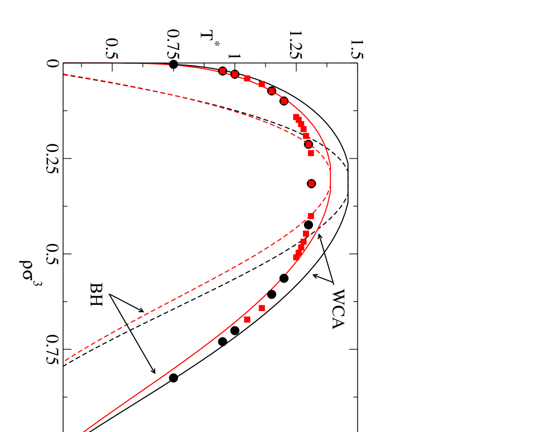
The equation of state of the bulk fluid was calculated using first-order thermodynamic perturbation theory using both the BH and WCA theories and the resulting phase diagrams are shown in Fig. 1. The Barker-Henderson theory gives somewhat low liquid densities and higher vapor densities with a lower critical point than does the WCA theory. Neithr theory is very accurate near the critical point where renormalization effects are expected to be important.

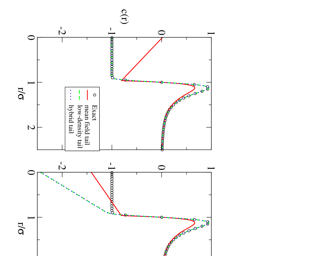
Figure 2 shows a comparison between the exact DCF at zero density and a reduced temperature of $T^{\ast}\equiv k_{B}T/\varepsilon=1.5$ and that of the model. In Fig, 2a, the model is evaluated using the exact second virial coefficient so that the low-density and hybrid tails reproduce the exact result. The error found in using the mean-field tail is due to compensation in the core for the errors made outside the core in the integral of the DCF. Note that the thermodynamic constraint depends on the spatial integral of the DCF times $r^{2}$ which explains the relatively large deviations required inside the core. Figure 2b shows the models as evaluated using the Barker-Henderson theory. Since the low-density free energy is incorrect in this theory, i.e. the second virial coefficient is wrong, the low-density and hybrid models now include spurious core corrections whereas the core correction for the mean-field tail is actually smaller. This is because the mean-field tail is very close to that which is used in the Barker-Henderson perturbation theory giving a case of compensating errors.

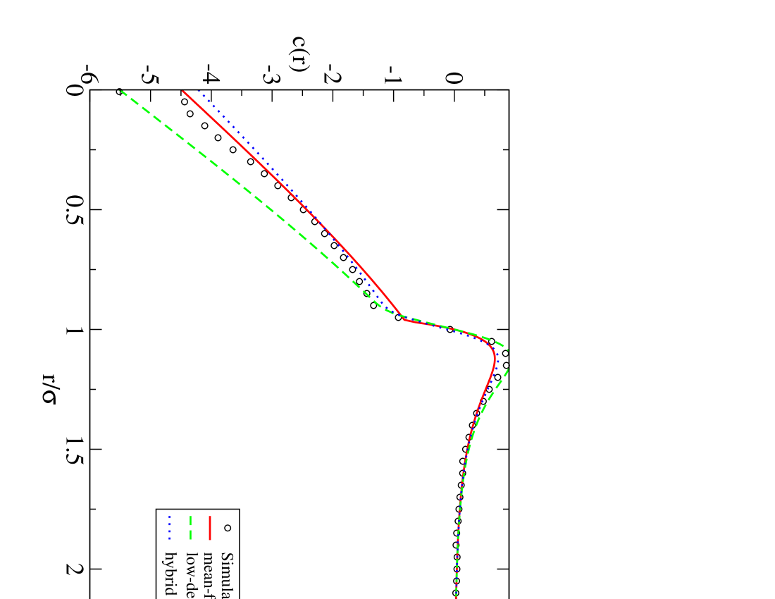
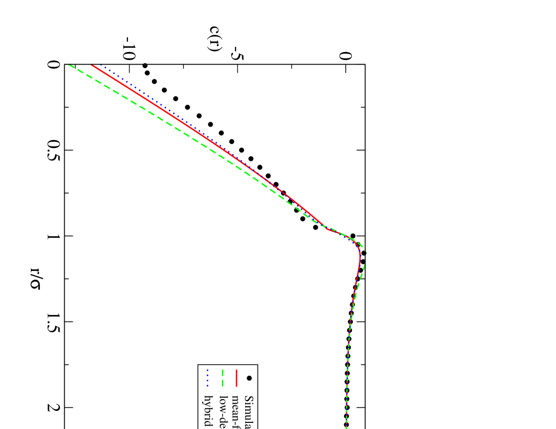
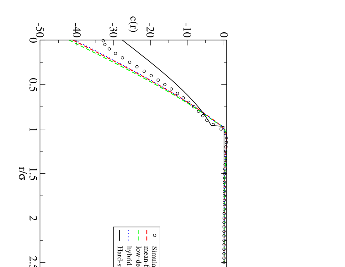
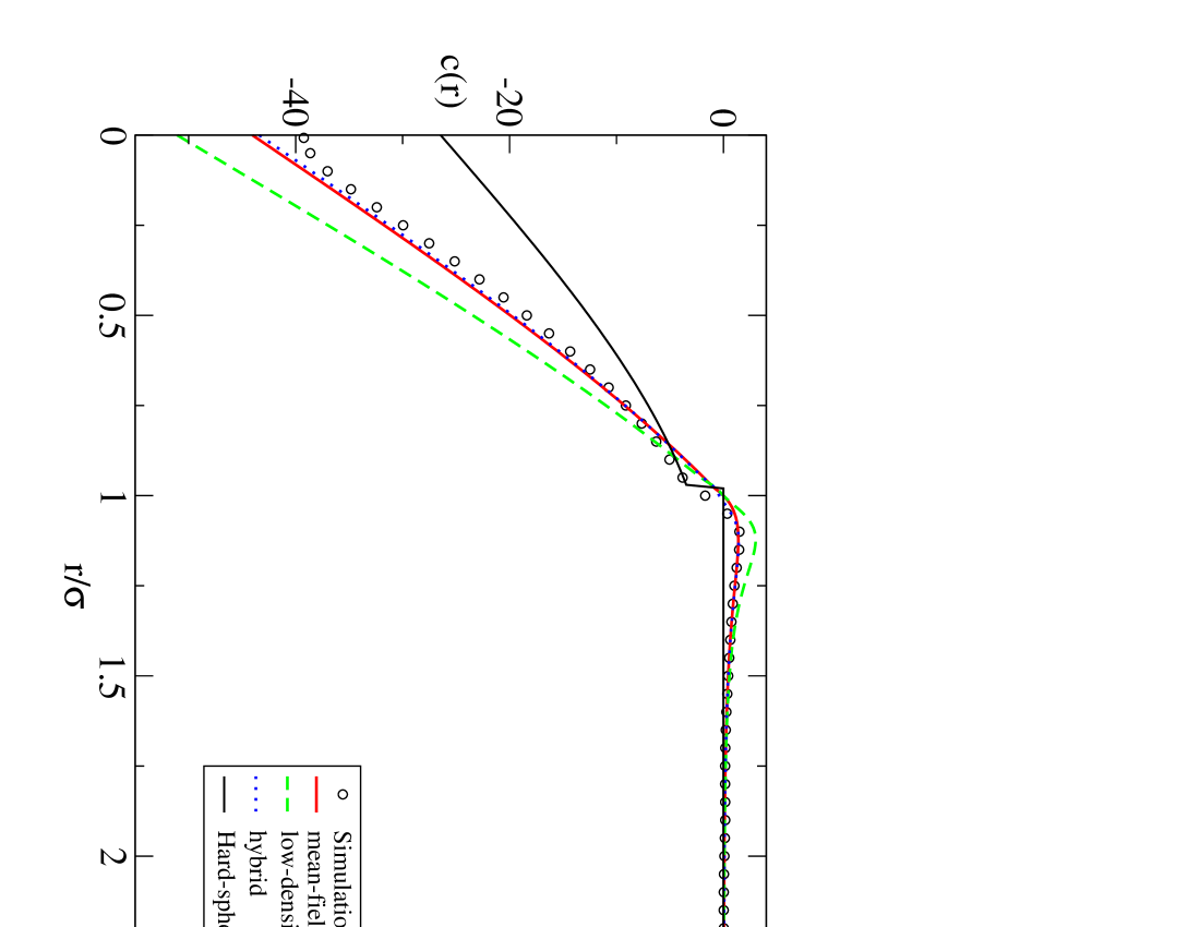
Figures (3)-(5) show the DCF for different densities for $T^{\ast}=1.5$ and Fig. (6) shows the DCF for $T^{\ast}=0.72$ and $\rho\sigma^{3}=0.72$ . While this simple model cannot be expected to be perfect, the figures show that it represents a good first approximation to the actual DCF. For the higher temperature, the low-density tail appears slightly better at the lowest density. At the lower temperature, the difference is greater. This is because the peak in the DFC is due to the minimum in the potential and the low density tail, due to the exponentiation of the potential, gives a higher peak than both the mean field tail and the data. In order to give the same integral, the core correction is therefore forced to be more negative. Altogether, it would appear that all of the tail approximations are reasonable. The low-density tail is better at low densities, the mean-field tail is better at high density and the hybrid model is overall the most accurate. Nevertheless, it would appear that the additional analytic complexity of the low-density and hybrid tails are only justified if the equation of state is exact at low density and if there is particular interest in reproducing the exact low-density DCF.

For the highest densities, see Figs.(5) and (6), the hard-sphere contribution to the DCF is also shown so as to highlight the role of the core correction. For $T^{\ast}=1.5$, the core correction gives a modest improvement over the hard-sphere DCF over most of the core region. The errors are largest at $r=0$ which is probably the least important region. On the other hand, for $T^{\ast}=0.72$, the core correction gives a clear improvement over the hard-sphere DCF throughout the entire core region.

IV Application to the planar interface

IV.1 Reduction to a one-dimensional problem

In this Section, the model DCF is used to evaluate the density functional theories discussed in Section II for the case of a planar liquid-vapor interface. The discussion here will focus on the extended mean-field approximation for the DCF with the mean-field tail. Calculations with the more complex models require more numerical analysis and confirm the conclusions of Section III that the additional complexity has little effect on the quantitative results.

The density is assumed to vary in only one direction, say the $z$ -direction, and to be constant in all other directions. For a fixed temperature below the critical point, there is a unique value of the liquid and vapor densities, $\overline{n}_{l}$ and $\overline{n}_{v}$ , such that the two phases have the same chemical potential and pressure and can therefore coexist. Within the LDCF model, the excess free energy per unit area, i.e. the surface tension, can be written as

$$\gamma\equiv\frac{1}{A}\left(\Omega\left[n\right]-\Omega\left(\overline{n}_{l}\right)\right) = \beta F_{ex}^{HS}\left[n\right]+\int_{-\infty}^{\infty}\left(\Delta f\left(n\left(z\right)\right)-\mu n\left(z\right)-\left(f\left(n_{l}\right)-\mu n_{l}\right)\right)dz$$

$$+\frac{1}{4}\int_{-\infty}^{\infty}\int_{-\infty}^{\infty}\left(n\left(z_{1}\right)-\overline{\rho}_{0}\right)\left(n\left(z_{1}\right)-n\left(z_{2}\right)\right)\widetilde{c}_{2}^{core}\left(z_{12};n\left(z_{1}\right),\overline{\rho}_{0}\right)dz_{2}dz_{1}$$

$$+\frac{1}{4}\int_{-\infty}^{\infty}\int_{-\infty}^{\infty}\left(n\left(z_{1}\right)-n\left(z_{2}\right)\right)^{2}\beta\widetilde{v}\left(z_{12}\right)dz_{2}dz_{1}$$

where

$$\widetilde{v}\left(z\right)\equiv\int_{-\infty}^{\infty}\int_{-\infty}^{\infty}v\left(r\right)\Theta\left(r-d\right)dxdy$$ (35)

and

$$\widetilde{c}_{2}^{core}\left(z;n,\overline{\rho}_{0}\right)\equiv\int_{-\infty}^{\infty}\int_{-\infty}^{\infty}\left(\overline{\overline{a}}_{0}\left(n,\overline{\rho}_{0}\right)+\overline{\overline{a}}_{1}\left(n,\overline{\rho}_{0}\right)\frac{r}{d}\right)\Theta\left(d-r\right)dxdy.$$ (36)

are the planar averages of the potential and the core correction to the DCF. The constants in the core term are related to those in the extended mean-field model by

$$\overline{\overline{a}}_{i}\left(n,\overline{\rho}_{0}\right)=2\int_{0}^{1}d\lambda\int_{0}^{\lambda}d\lambda^{\prime}\;a_{i}\left(\overline{\rho}_{0}+\lambda^{\prime}\left(n-\overline{\rho}_{0}\right)\right).$$ (37)

Note that the equivalent of the model of ESS is obtained by the substitution $\overline{\overline{a}}_{i}\left(n,\overline{\rho}_{0}\right)\rightarrow\frac{1}{2}a_{i}\left(n\right)$ whereas that of Tang results from $\overline{\overline{a}}_{i}\left(n,\overline{\rho}_{0}\right)\rightarrow a_{i}\left(\overline{\rho}_{0}\right)$ together with the specific choice $\overline{\rho}_{0}=\frac{1}{2}\left(\overline{n}_{l}+\overline{n}_{v}\right)$. The equilibrium density profile is found by minimizing the free energy with respect to the density profile subject to the boundary conditions

$$\lim_{z\rightarrow-\infty}n\left(z\right) = n_{l}\left(\mu,T\right)$$ (38)

$$\lim_{z\rightarrow\infty}n\left(z\right) = n_{v}\left(\mu,T\right)$$

$$\lim_{z\rightarrow\pm\infty}\frac{d}{dz}n\left(z\right) = 0.$$

IV.2 Implementation

The numerical work begins with the calculation of the Barker-Henderson hard-sphere diameter, $d(T)$, from eq.(28). The coefficients $a_{i}\left(n\right)$ are evaluated for 100 points in the density range $0\leq n\sigma^{3}\leq 1$ using either the BH or WCA first order perturbation theories. They are then interpolated using cubic splines which permit easy calculation of the coefficients $\overline{\overline{a}}_{i}\left(n,\overline{\rho}_{0}\right)$ for a given value of $\overline{\rho}_{0}$. (In this regard, the difference in computational complexity between the LDCF theory and the approximations of ESS and Tang is minimal.) The calculation of the free energy is discretized by introducing a lattice of points on the interval $[-L,L]$ via $z_{i}=-L+i\delta$ for $i=0$ to $N=2L/\delta$. The limits are chosen sufficiently large that it may be assumed that $n\left(L\right)=n_{v}$ and $n\left(-L\right)=n_{l}$ and the goal is to find the profile in the form of the points $n_{i}=n\left(z_{i}\right)$ which minimize the free energy functional. (Although care must be taken to include the contributions of the regions outside this range, which can be done analytically.) The minimimization of the free energy was performed using the Broyden-Fletcher-Goldfarb-Shanno quasi-Newton method as implemented in the GNU Scientific LibraryGSL . Except where otherwise noted, all results reported here are based on a lattice of $20$ points per hard-sphere diameter, $\delta=d/20$.

IV.3 Results

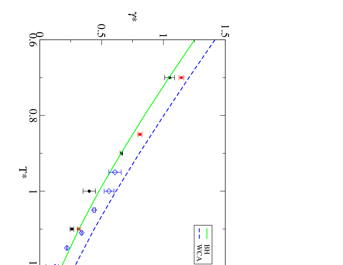
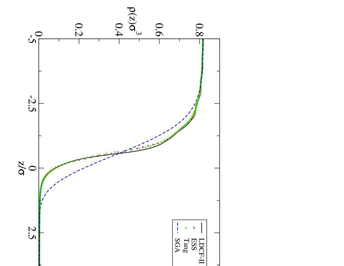
Figure 7 shows the reduced surface tension, $\gamma^{\ast}=\gamma\sigma^{2}/\varepsilon$ as a function of temperature obtained using the LDC-II with both the BH and WCA first order perturbation theories for the equations of state, as well as the simulation results of Mecke, Winkelmann and FischerMecke et al. (1997) of Duque, Pamies and VegaDuque et al. (2004) and of Potoff and PanagiotopoulosPotoff and Panagiotopoulos (2000). The surface tensions calculated are quite sensitive to the densities of the coexisting phases so, as might be guessed from the phase diagrams, the BH results are more accurate at higher temperatures, near the critical point, whereas at the lowest temperatures, the results using both perturbation theories are comparable. Figure 8 shows the density profiles obtained for $T^{\ast}=0.7$ calculated using all of the various DFTs discussed above. The SGA gives a much broader profile than the other DFTs. The LDCF and Tang models give smooth profiles while the ESS shows some small oscillations at the transition to high density, but the profiles for all four models are extremely similar. They all show a very rapid increase in density moving from the vapor into the liquid, followed by a slower, more rounded profile as the density approaches that of the liquid.

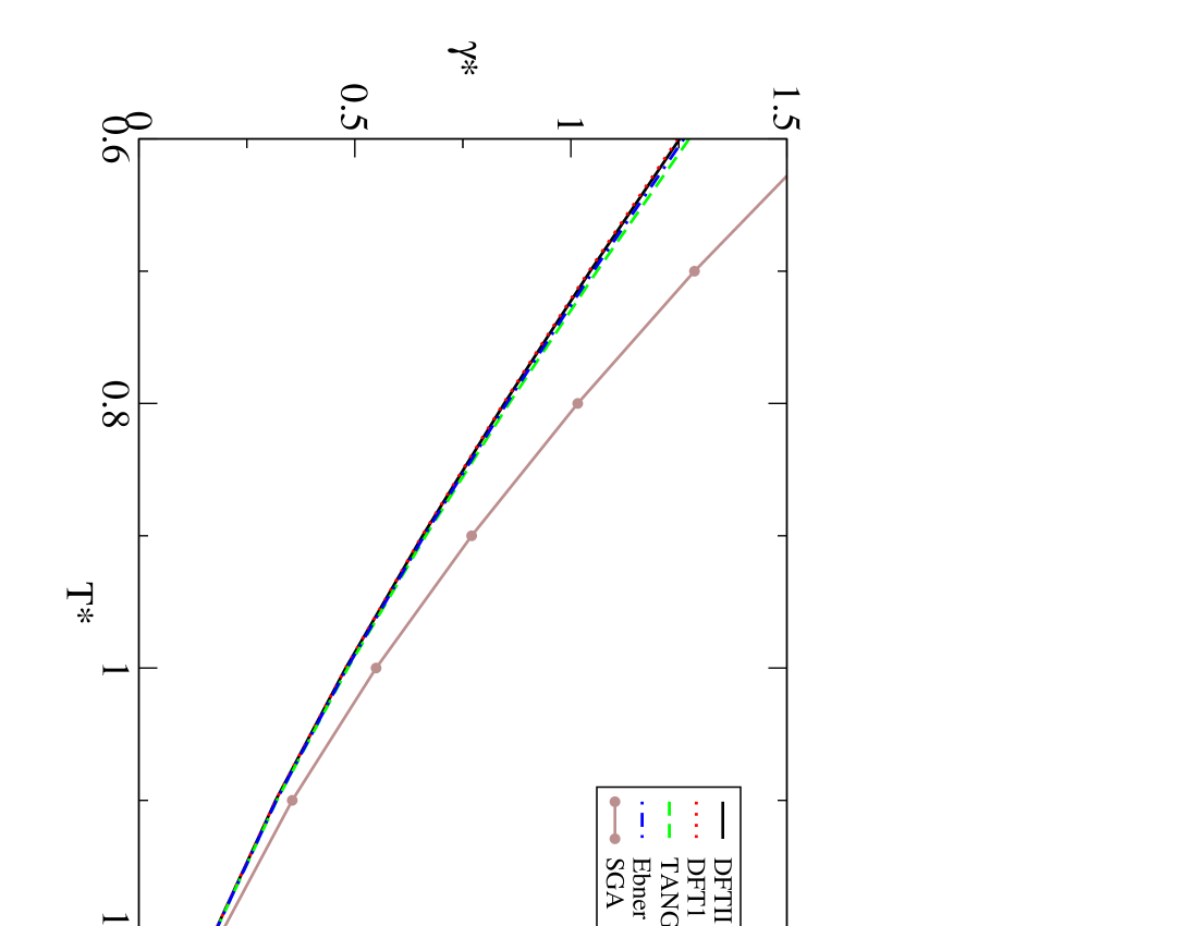
Figure 9 shows a comparison of several different versions of the DFT including the LDCF-I, eq.(11), the LDCF-II,eq.(12), and the approximate theories of ESS type, Tang and the Square-Gradient Approximation (SGA). With one exception, all of the DFTs except the SGA give almost identical results. The SGA gives a considerably higher surface tension, a fact well-known in the literatureCornelisse et al. (1997). The exception is that in the present calculations, the ESS theory is unstable at $T^{\ast}=0.6$ and no solution was found.

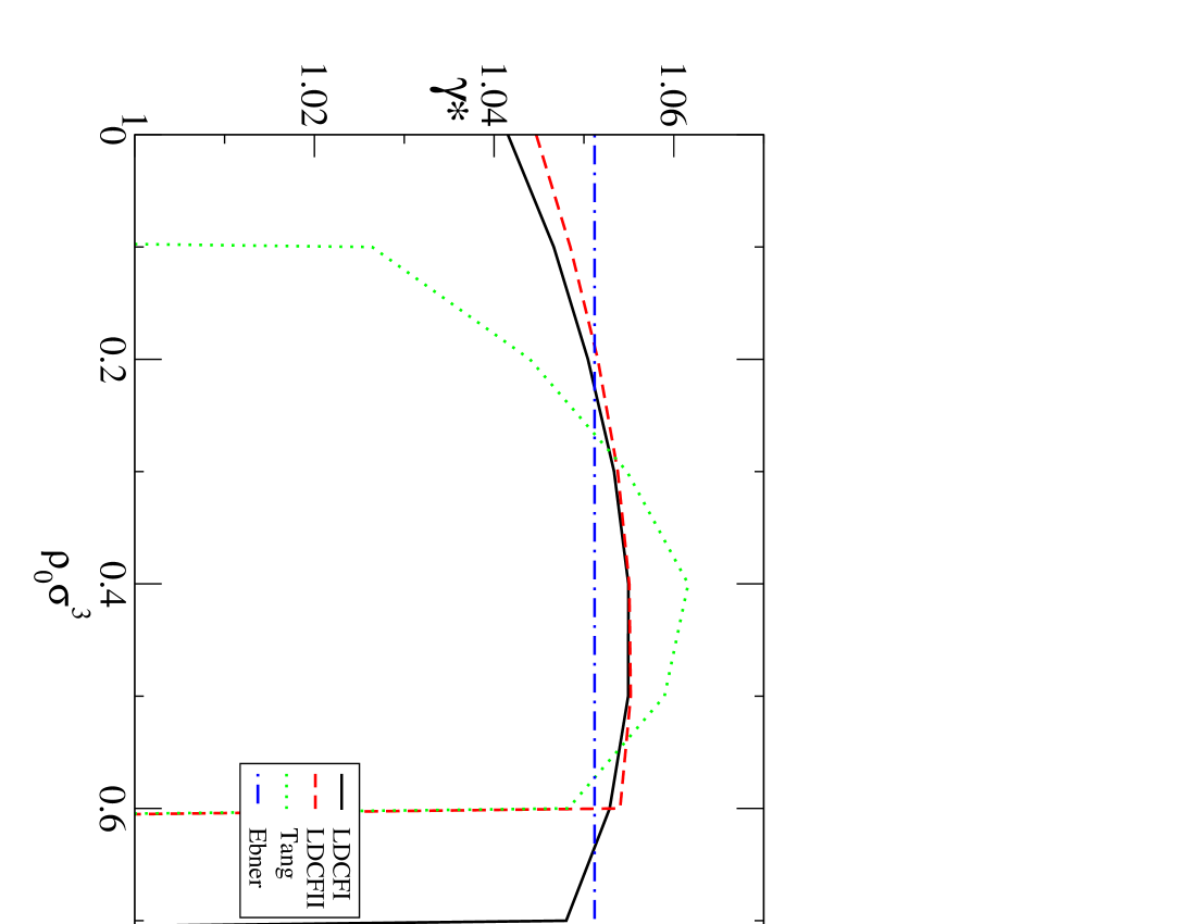
The exact free energy is independent of the path in density space used to calculate it. This property is shared in the ESS-type theory but the other approximate DFTs all contain an explicit dependence on the reference density. Figure 10 shows the variation of the surface tension as a function of the reference density for $T^{\ast}=0.7$ . Note that the LDCF approximations as well as that of Tang do not give stable solutions if the reference density is chosen too large. Within the region that solutions exist, the resulting free energies are in fact only weakly sensitive to the value of the reference density, with the Tang theory showing the largest variation. The LDCF-I theory is the most robust in the sense of possessing the widest range of possible values of reference density.

One interesting distinction between the theories is the range of temperatures for which they give stable solutions. The liquid-vapor interface only exists for temperatures below the critical point (around $T^{\ast}=1.3$ in simulation and the BH theory). As the temperature is lowered, the system eventually reaches the triple point, at about $T^{\ast}=0.7$, below which the thermodynamically stable phases are the vapor and the solid. However, the liquid can still exist as a metastable phase and indeed, the usual perturbation theories continue to work for temperatures much lower than the triple point. It is therefore of interest to check the behavior of the DFT’s for lower temperatures where a metastable liquid-vapor interface is possible. In fact, both of the LDCF theories continue to give sensible results for temperatures as low as $T^{\ast}=0.25$ as does the model of Tang. On the other hand, attempts to solve the ESS-theory below the triple point are problematic. Calculations performed at $T^{\ast}=0.6$ with the ESS are stable but the profile shows significant oscillations. However, when the density of lattice points is doubled, it is no longer possible to find a stable solution and this is true at lower temperatures, even using the original lattice spacing. For comparison, halving the lattice spacing has no qualitative affect on the LDCF calculations, even at the lowest temperature and the surface tension changes by less than $0.2\%$.

V Conclusions

The extended mean field model for the DCF, consisting of a hard-core contribution, a mean-field tail and a linear core correction, has been shown to be a reasonable approximation to the DCF for a Lennard-Jones fluid. The model retains much of the simplicity of the mean-field model but is constructed to give a faithful representation of the thermodynamics of the homogeneous system. The approach used here differs somewhat from that commonly found in the literature wherein the goal is to make an ab initio ansatz for DCF, or more generally, for the DFT, which is subsequently tested by comparing its prediction of the properties of the homogeneous system to simulation. Given that good, computationally efficient means exist - and have long existed - for calculating such properties, there is no real reason to try to construct a DFT at this level. Instead, the philosophy used here is to view DFT as a to0l which is primarily useful for studying more complex inhomogeneous systems and which, as such, is legitimately constructed assuming a priori knowledge of the homogeneous system.

In this paper, the model DCF was used in conjunction with several approximate DFTs to study the liquid-vapor interface of a Lennard-Jones fluid. It was found that aside from the well-known exception of the SGA, all of the DFTs gave very similar results for both the surface tension and the density profile. The calculated surface tensions were also found to agree well with the results from simulations.

It was noted at several points that the different approximate DFT’s were sometimes unstable in the sense that no smooth density profile could be obtained. Fundamentally, this is due to the fact that the hard-sphere part of the free energy, described by FMT, involves smoothed-densities while the attractive part of the free energy involves the density evaluated at a point. The instabilities arise because a very localized spike in the density can increase the size of the attractive part of the free energy whereas, because of the smoothing, it has little effect on the hard-sphere contribution. This defect of the LDCF theories will be explored further in a future publication. Further applications of this work will be to the study of different potential models and geometries, particularly the case of anisotropic potentials.

Appendix A
Proof of eq.(II.2)

To prove eq.(II.2), the two-body term is written as

$$-\frac{1}{2}\int_{V}\int_{V}\left(n\left(\mathbf{r}_{1}\right)-\overline{\rho}_{0}\right)\left(n\left(\mathbf{r}_{2}\right)-n\left(\mathbf{r}_{1}\right)\right)\Delta\overline{\overline{c}}_{2}\left(r_{12};n\left(\mathbf{r}_{1}\right),\overline{\rho}_{0}\right)d\mathbf{r}_{1}d\mathbf{r}_{2}$$

$$= \frac{1}{4}\int_{V}\int_{V}\left(n\left(\mathbf{r}_{2}\right)-n\left(\mathbf{r}_{1}\right)\right)^{2}\Delta\overline{\overline{c}}_{2}\left(r_{12};n\left(\mathbf{r}_{1}\right),\overline{\rho}_{0}\right)d\mathbf{r}_{1}d\mathbf{r}_{2}$$

$$-\frac{1}{2}\int_{V}\int_{V}\left(\frac{n\left(\mathbf{r}_{1}\right)+n\left(\mathbf{r}_{2}\right)}{2}-\overline{\rho}_{0}\right)\left(n\left(\mathbf{r}_{2}\right)-n\left(\mathbf{r}_{1}\right)\right)\Delta\overline{\overline{c}}_{2}\left(r_{12};\frac{n\left(\mathbf{r}_{1}\right)+n\left(\mathbf{r}_{2}\right)}{2}+\frac{n\left(\mathbf{r}_{1}\right)-n\left(\mathbf{r}_{2}\right)}{2},\overline{\rho}_{0}\right)d\mathbf{r}_{1}d\mathbf{r}_{2}$$

Expanding in the difference in densities gives

$$\Delta\overline{\overline{c}}_{2}\left(r_{12};\frac{n\left(\mathbf{r}_{1}\right)+n\left(\mathbf{r}_{2}\right)}{2}+\frac{n\left(\mathbf{r}_{1}\right)-n\left(\mathbf{r}_{2}\right)}{2},\overline{\rho}_{0}\right)$$

$$= \int_{0}^{1}dx\left(1-x\right)\Delta c_{2}\left(r_{12};\overline{\rho}_{0}+x\left(\frac{n\left(\mathbf{r}_{1}\right)+n\left(\mathbf{r}_{2}\right)}{2}+\frac{n\left(\mathbf{r}_{1}\right)-n\left(\mathbf{r}_{2}\right)}{2}-\overline{\rho}_{0}\right)\right)$$

$$= \Delta\overline{\overline{c}}_{2}\left(r_{12};\frac{n\left(\mathbf{r}_{1}\right)+n\left(\mathbf{r}_{2}\right)}{2},\overline{\rho}_{0}\right)$$

$$+\left(\frac{n\left(\mathbf{r}_{1}\right)-n\left(\mathbf{r}_{2}\right)}{2}\right)\int_{0}^{1}dx\left(1-x\right)x\left.\frac{\partial\Delta\overline{\overline{c}}_{2}\left(r_{12};n\right)}{\partial n}\right|_{\overline{\rho}_{0}+x\left(\frac{n\left(\mathbf{r}_{1}\right)+n\left(\mathbf{r}_{2}\right)}{2}-\overline{\rho}_{0}\right)}$$

$$+O\left(\frac{n\left(\mathbf{r}_{1}\right)-n\left(\mathbf{r}_{2}\right)}{2}\right)^{2}$$

The second term is

$$\int_{0}^{1}dx\left(1-x\right)x\left.\frac{\partial\Delta\overline{\overline{c}}_{2}\left(r_{12};n\right)}{\partial n}\right|_{\overline{\rho}_{0}+x\left(\frac{n\left(\mathbf{r}_{1}\right)+n\left(\mathbf{r}_{2}\right)}{2}-\overline{\rho}_{0}\right)}$$

$$= \left(\frac{n\left(\mathbf{r}_{1}\right)+n\left(\mathbf{r}_{2}\right)}{2}-\overline{\rho}_{0}\right)^{-1}\int_{0}^{1}dx\left(1-x\right)x\frac{\partial}{\partial x}\Delta c_{2}\left(r_{12};\overline{\rho}_{0}+x\left(\frac{n\left(\mathbf{r}_{1}\right)+n\left(\mathbf{r}_{2}\right)}{2}-\overline{\rho}_{0}\right)\right)$$

$$= \left(\frac{n\left(\mathbf{r}_{1}\right)+n\left(\mathbf{r}_{2}\right)}{2}-\overline{\rho}_{0}\right)^{-1}\int_{0}^{1}dx\left(-1+2x\right)\Delta c_{2}\left(r_{12};\overline{\rho}_{0}+x\left(\frac{n\left(\mathbf{r}_{1}\right)+n\left(\mathbf{r}_{2}\right)}{2}-\overline{\rho}_{0}\right)\right)$$

So

$$-\frac{1}{2}\int_{V}\int_{V}\left(n\left(\mathbf{r}_{1}\right)-\overline{\rho}_{0}\right)\left(n\left(\mathbf{r}_{2}\right)-n\left(\mathbf{r}_{1}\right)\right)\Delta\overline{\overline{c}}_{2}\left(r_{12};n\left(\mathbf{r}_{1}\right),\overline{\rho}_{0}\right)d\mathbf{r}_{1}d\mathbf{r}_{2}$$

$$= \frac{1}{4}\int_{V}\int_{V}\left(n\left(\mathbf{r}_{2}\right)-n\left(\mathbf{r}_{1}\right)\right)^{2}\int_{0}^{1}dx\left(1-x\right)\Delta c_{2}\left(r_{12};\overline{\rho}_{0}+x\left(\frac{n\left(\mathbf{r}_{1}\right)+n\left(\mathbf{r}_{2}\right)}{2}-\overline{\rho}_{0}\right)\right)$$

$$-\frac{1}{2}\int_{V}\int_{V}\left(\frac{n\left(\mathbf{r}_{1}\right)+n\left(\mathbf{r}_{2}\right)}{2}-\overline{\rho}_{0}\right)\left(n\left(\mathbf{r}_{2}\right)-n\left(\mathbf{r}_{1}\right)\right)\Delta\overline{\overline{c}}_{2}\left(r_{12};\frac{n\left(\mathbf{r}_{1}\right)+n\left(\mathbf{r}_{2}\right)}{2},\overline{\rho}_{0}\right)d\mathbf{r}_{1}d\mathbf{r}_{2}$$

$$+\frac{1}{4}\int_{V}\int_{V}\left(n\left(\mathbf{r}_{2}\right)-n\left(\mathbf{r}_{1}\right)\right)^{2}\int_{0}^{1}dx\left(-1+2x\right)\Delta c_{2}\left(r_{12};\overline{\rho}_{0}+x\left(\frac{n\left(\mathbf{r}_{1}\right)+n\left(\mathbf{r}_{2}\right)}{2}-\overline{\rho}_{0}\right)\right)$$

$$+O\left(\frac{n\left(\mathbf{r}_{1}\right)-n\left(\mathbf{r}_{2}\right)}{2}\right)^{3}$$

The second term on the right is odd under an interchange of the indices and so vanishes. What is left gives

$$-\frac{1}{2}\int_{V}\int_{V}\left(n\left(\mathbf{r}_{1}\right)-\overline{\rho}_{0}\right)\left(n\left(\mathbf{r}_{2}\right)-n\left(\mathbf{r}_{1}\right)\right)\Delta\overline{\overline{c}}_{2}\left(r_{12};n\left(\mathbf{r}_{1}\right),\overline{\rho}_{0}\right)d\mathbf{r}_{1}d\mathbf{r}_{2}$$

$$= \frac{1}{4}\int_{V}\int_{V}\left(n\left(\mathbf{r}_{2}\right)-n\left(\mathbf{r}_{1}\right)\right)^{2}\int_{0}^{1}x\Delta c_{2}\left(r_{12};\overline{\rho}_{0}+x\left(\frac{n\left(\mathbf{r}_{1}\right)+n\left(\mathbf{r}_{2}\right)}{2}-\overline{\rho}_{0}\right)\right)dx$$

$$+O\left(\frac{n\left(\mathbf{r}_{1}\right)-n\left(\mathbf{r}_{2}\right)}{2}\right)^{3}$$

The expression for the free energy is thus

$$\beta F_{ex}\left[n\right] = \beta F_{ex}^{HS}\left[n\right]+\int d\mathbf{r}\;\Delta f\left(n\left(\mathbf{r}\right)\right)$$

$$+\frac{1}{4}\int_{V}\int_{V}\left(n\left(\mathbf{r}_{1}\right)-n\left(\mathbf{r}_{2}\right)\right)^{2}\Delta c_{2}^{tail}\left(r_{12}\right)d\mathbf{r}_{2}d\mathbf{r}_{1}$$

$$+\frac{1}{4}\int_{V}\int_{V}\left(n\left(\mathbf{r}_{1}\right)-n\left(\mathbf{r}_{2}\right)\right)^{2}\left[2\int_{0}^{1}\lambda\Delta c_{2}^{core}\left(r_{12};\overline{\rho}_{0}+\lambda\left(\frac{n\left(\mathbf{r}_{1}\right)+n\left(\mathbf{r}_{2}\right)}{2}-\overline{\rho}_{0}\right)\right)d\lambda\right]d\mathbf{r}_{1}d\mathbf{r}_{2}$$

$$+O\left(\frac{n\left(\mathbf{r}_{1}\right)-n\left(\mathbf{r}_{2}\right)}{2}\right)^{3}$$

or

$$\beta F_{ex}\left[n\right] = \beta F_{ex}^{HS}\left[n\right]+\int d\mathbf{r}\;\Delta f\left(n\left(\mathbf{r}\right)\right)$$

$$+\frac{1}{4}\int_{V}\int_{V}\left(n\left(\mathbf{r}_{1}\right)-n\left(\mathbf{r}_{2}\right)\right)^{2}\left[2\int_{0}^{1}\lambda\Delta c_{2}\left(r_{12};\overline{\rho}_{0}+\lambda\left(\frac{n\left(\mathbf{r}_{1}\right)+n\left(\mathbf{r}_{2}\right)}{2}-\overline{\rho}_{0}\right)\right)d\lambda\right]d\mathbf{r}_{1}d\mathbf{r}_{2}$$

$$+O\left(\frac{n\left(\mathbf{r}_{1}\right)-n\left(\mathbf{r}_{2}\right)}{2}\right)^{3}$$

Appendix B Figure captions

Fig.1. The coexistence curve for the Lennard-Jones fluid as calculated using both the WCA perturbation theory and the BH theory. The full lines are the liquid-vapor coexistence curves, the dashed-lines are the spinodals and the symbols are the simulation data from ref.Hansen and Verlet (1969)(circles) and from ref. Potoff and Panagiotopoulos (2000) (squares).

Fig. 2. The DCF at zero density and $T^{\ast}=1.5$. The symbols are the the negative of the Meyer function (the exact result for zero density), and the lines are from the three choices of tail function described in the text. Figure (a) is based on the exact equation of state while in Fig.(b), the Barker-Henderson perturbation theory is used.

Fig. 3. The DCF at $T^{\ast}=1.5$ and $\rho\sigma^{3}=0.4$ as determined from the model using the Barker-Henderson perturbation theory, lines, and the simulation data of Llano-Restrepo and ChapmanLlano-Restrepo and Chapman (1992).

Fig. 4. The DCF at $T^{\ast}=1.5$ and $\rho\sigma^{3}=0.6$ as determined from the model using the Barker-Henderson perturbation theory, lines, and the simulation data of Llano-Restrepo and ChapmanLlano-Restrepo and Chapman (1992).

Fig. 5. The DCF at $T^{\ast}=1.5$ and $\rho\sigma^{3}=0.9$ as determined from the model using the Barker-Henderson perturbation theory, lines, and the simulation data of Llano-Restrepo and ChapmanLlano-Restrepo and Chapman (1992). The hard-sphere contribution to the DCF is shown in black.

Fig. 6. The DCF at $T^{\ast}=0.72$ and $\rho\sigma^{3}=0.85$ as determined from the model using the Barker-Henderson perturbation theory, lines, and the simulation data of Llano-Restrepo and ChapmanLlano-Restrepo and Chapman (1992).The hard-sphere contribution to the DCF is shown in black.

Fig. 7. The surface tension as a function of temperature. The symbols are measurements from simulations (circles from ref.Duque et al. (2004),squares from ref.Mecke et al. (1997) and triangles from ref. Potoff and Panagiotopoulos (2000)). The lines are from the LDCF-II DFT evaluated with the corrected mean-field DCF using the equation of state calculated from the BH perturbation theory (full line) and the WCA theory (broken line).

Fig. 8. The density profiles calculated from the various DFTs for $T^{\ast}=0.7$.

Fig. 9. A comparison of the surface tension as a function of reduced temperature as calculated from the LDCF-II, ESS, Tang and SGA DFTs.

Fig. 10. The variation of the reduced surface tension, $\gamma^{\ast}$ as a function of the reference density $\rho_{0}\sigma^{3}$ for the different DFTs using the BH equation of state and for $T^{\ast}=0.7$. The vertical lines are the boundary of the region for which a stable solution was found.

Figure 1:

Figure 2:

Figure 3:

Figure 4:

Figure 5:

Figure 6:

Figure 7:

Figure 8:

Figure 9:

Figure 10:

References

- van der Waals (1894) J. D. van der Waals, Z. Phys. Chem. 13, 657 (1894).
- Rowlinson (1979) J. S. Rowlinson, J. Stat. Phys. 20, 197 (1979).
- Evans (1979) R. Evans, Adv. Phys. 28, 143 (1979).
- Rowlinson and Widom (2002) J. S. Rowlinson and B. Widom, Molecular Theory of Capillarity (Dover Publications, N. Y., 2002).
- Lutsko (2006) J. F. Lutsko, Physica A 366, 229 (2006).
- Cahn and Hilliard (1958) J. W. Cahn and J. E. Hilliard, J. Chem. Phys. 28, 258 (1958).
- Ebner et al. (1976) C. Ebner, W. F. Saam, and D. Stroud, Phys. Rev. A 14, 2264 (1976).
- Saam and Ebner (1977) W. F. Saam and C. Ebner, Phys. Rev. A 15, 2566 (1977).
- Tang et al. (1991) Z. Tang, L. E. Scriven, and H. T. Davis, J. Chem. Phys. 95, 2659 (1991).
- Wadewitz and Winkelmann (2000) T. Wadewitz and J. Winkelmann, J. Chem. Phys. 113, 2447 (2000).
- Tang and Wu (2003) Y. Tang and J. Wu, J. Chem. Phys. 119, 7388 (2003).
- Tang and Wu (2004) Y. Tang and J. Wu, Phys. Rev. E 70, 011201 (2004).
- Tang (2005) Y. Tang, J. Chem. Phys. 123, 204704 (2005).
- Hoye and Blum (1977) J. Hoye and L. Blum, J. Stat. Phys. 16, 399 (1977).
- Tang (2003) Y. Tang, J. Chem. Phys. 118, 4140 (2003).
- Tang (2004) Y. Tang, J. Chem. Phys. 121, 21 (2004).
- Rosenfeld (1989) Y. Rosenfeld, Phys. Rev. Lett. 63, 980 (1989).
- Rosenfeld et al. (1990) Y. Rosenfeld, D. Levesque, and J.-J. Weis, J. Chem. Phys. 92, 6818 (1990).
- Tarazona (2000) P. Tarazona, Phys. Rev. Lett. 84, 694 (2000).
- Roth et al. (2002) R. Roth, R. Evans, A. Lang, and G. Kahl, J. Phys.: Cond. Matt. 14, 12063 (2002).
- Cornelisse et al. (1997) P. M. W. Cornelisse, C. J. Peters, and J. de Swaan Arons, J. Chem. Phys. 106, 9820 (1997).
- Duque et al. (2004) D. Duque, J. C. Pamies, and L. F. Vega, J. Chem. Phys. 121, 11395 (2004).
- Llano-Restrepo and Chapman (1992) M. Llano-Restrepo and W. G. Chapman, J. Chem. Phys. 97, 2046 (1992).
- Rogers and Young (1984) F. J. Rogers and D. A. Young, Phys. Rev. A 30, 999 (1984).
- Zerah and Hansen (1986) G. Zerah and J. P. Hansen, J. Chem. Phys. 84, 2336 (1986).
- Rosenfeld (1993) Y. Rosenfeld, J. Chem. Phys. 98, 8126 (1993).
- Barker and Henderson (1967a) J. A. Barker and D. Henderson, J. Chem. Phys. 47, 4714 (1967a).
- Hansen and McDonald (1986) J.-P. Hansen and I. McDonald, Theory of Simple Liquids (Academic Press, San Diego, Ca, 1986).
- Paricaud (2006) P. Paricaud, J. Chem. Phys. 124, 154505 (2006).
- Chandler and Weeks (1970) D. Chandler and J. D. Weeks, Phys. Rev. Lett. 25, 149 (1970).
- Chandler et al. (1971) D. Chandler, J. D. Weeks, and H. C. Andersen, J. Chem. Phys. 54, 5237 (1971).
- Andersen et al. (1971) H. C. Andersen, D. Chandler, and J. D. Weeks, Phys. Rev. A 4, 1597 (1971).
- Stell and Penrose (1983) G. Stell and O. Penrose, Phys. Rev. Lett. 51, 1397 (1983).
- Barker and Henderson (1967b) J. A. Barker and D. Henderson, J. Chem. Phys. 47, 2856 (1967b).
- Barker and Henderson (1976) J. A. Barker and D. Henderson, Rev. Mod. Phys. 48, 587 (1976).
- (36) The gnu scientific library, eprint http://sources.redhat.com/gsl.
- Mecke et al. (1997) M. Mecke, J. Winkelmann, and J. Fischer, J. Chem. Phys. 107, 9264 (1997).
- Potoff and Panagiotopoulos (2000) J. J. Potoff and A. Z. Panagiotopoulos, J. Chem. Physics 112, 6411 (2000).
- Hansen and Verlet (1969) J. P. Hansen and L. Verlet, Phys. Rev. 184, 151 (1969).