Unbiased estimates of galaxy scaling relations from photometric redshift surveys

Abstract

Many physical properties of galaxies correlate with one another, and these correlations are often used to constrain galaxy formation models. Such correlations include the color-magnitude relation, the luminosity-size relation, the Fundamental Plane, etc. However, the transformation from observable (e.g. angular size, apparent brightness) to physical quantity (physical size, luminosity), is often distance-dependent. Noise in the distance estimate will lead to biased estimates of these correlations, thus compromising the ability of photometric redshift surveys to constrain galaxy formation models. We describe two methods which can remove this bias. One is a generalization of the $V_{\rm max}$ method, and the other is a maximum likelihood approach. We illustrate their effectiveness by studying the size-luminosity relation in a mock catalog, although both methods can be applied to other scaling relations as well. We show that if one simply uses photometric redshifts one obtains a biased relation; our methods correct for this bias and recover the true relation.

1 Introduction

The ‘configuration space’ we use to describe galaxies is large, but galaxies do not fill it. The luminosity, color, size, surface brightness, stellar velocity dispersion, morphology, stellar mass, star formation history and spectral energy distribution of a galaxy are all correlated with one another. These correlations encode important information about galaxy formation, and so quantifying them provides important constraints on models.

Current (e.g. SDSS, Combo-17, MUSYC, Cosmos) and planned surveys (e.g. DES, LSST, SNAP) go considerably deeper in multicolor photometry than in spectroscopy, or are entirely photometric. For such surveys, reasonably accurate photometric redshift estimates are or will be made. The question then arises as to which galaxy observables and correlations are affected by the noisy distance estimate associated with a photometric rather than spectroscopic redshift. The most widely studied property is luminosity - clearly, errors in the distance result in incorrect luminosity estimates. If not accounted for, this leads to a biased estimate of the luminosity function (e.g. Subbarao et al. 1996). Hence, there has been considerable effort devoted to the question of how to correct for this bias (e.g. Chen et al. 2003), and the problem has now been solved (Sheth 2007).

The next step is to recover an unbiased estimate of not just the luminosity function, but the joint distribution of luminosity, color, size, etc., from photometric redshift datasets. The main goal of the present work is to provide an algorithm which does this for a magnitude limited photometric redshift survey. Because the same distance error which leads to a mis-estimate of the luminosity will produce a correlated mis-estimate of the size, we have chosen to phrase the discussion in terms of the size-luminosity relation - it exhibits all the features of interest.

Section 2 illustrates the nature of the problem by showing the bias in the size-luminosity relation which results from treating photometric redshifts as though they were spectroscopic redshifts. This is done by constructing a mock galaxy sample and then perturbing the true redshifts to mimic photometric redshift errors. Section 3 places this problem in the more general context of inverse problems in statistical astronomy, and argues that a deconvolution algorithm, such as that due to Lucy (1974), is well-suited to removing the bias. It shows the result of applying this non-parametric deconvolution technique to a mock galaxy sample. Section 4 provides a maximum-likelihood formulation and solution of the problem. A final section summarizes our findings and discusses possible further studies and applications.

Where necessary, we write the Hubble constant as $H_{0}=100h~{}{\rm km~{}s}^{-1}~{}{\rm Mpc}^{-1}$, and we assume a spatially flat cosmological model with $(\Omega_{M},\Omega_{\Lambda},h)=(0.3,0.7,0.7)$, where $\Omega_{M}$ and $\Omega_{\Lambda}$ are the present-day densities of matter and cosmological constant scaled to the critical density. We use $D_{\rm L}(z)$ to denote the luminosity distance; the angular diameter distance is $D_{\rm A}(z)=D_{\rm L}(z)/(1+z)^{2}$.

2 Correlations with observables: effect of distance errors

Figure 1: Distribution of spectroscopic and photometric redshifts in our mock catalog which was set-up to mimic the SDSS early-type galaxy sample. Contours show levels which are $1/2^{n}$ times the height of the maximum value, with $n$ running from 1 to 5. The photo-$z$ error distribution was assumed to follow equation (1).

In what follows, we use the luminosity-size relation to illustrate how photo-$z$ errors lead to biases.

We begin by generating a magnitude-limited mock galaxy catalog with parameters chosen to mimic those of SDSS early-type galaxies in the $g$ band, following the method given by Bernardi et al. (2003). The redshift range is restricted to the interval $0.01\leq z\leq 0.3$. We ignored passive evolution of the luminosities and colors, as well as K-corrections. The simulated magnitude-limited catalog has a similar ${\rm d}N/{\rm d}z$ distribution to that observed, and the distribution of apparent magnitudes, angular sizes, and velocity dispersions are very similar to those in the real data.

We then model photometric redshifts $\zeta$ by assuming that

$$p\big{[}D_{\rm L}(\zeta)|D_{\rm L}(z)\big{]}\,{\rm d}D_{\rm L}(\zeta)=\frac{{\rm d}x}{x}\,(\gamma x)^{\gamma}\,\frac{\exp(-\gamma x)}{\Gamma(\gamma)},$$ (1)

where $x=D_{\rm L}(\zeta)/D_{\rm L}(z)$ is the ratio of the photo-$z$ based luminosity distance to the true one, and $\gamma=5$. This distribution has $\langle x\rangle=1$ and $\sigma_{x}^{2}=1/\gamma$. With $\gamma=5$, this error distribution is substantially worse than typical photometric redshift errors. Figure 1 compares $\zeta$ and $z$. Note that the analysis which follows is not tied to this functional form for the photo-$z$ error distribution; we are simply using it to illustrate our methods.

In what follows, we use $M$ to denote the true absolute magnitude, and ${\cal M}$ to denote that estimated using $\zeta$ rather than $z$. And, with some abuse of notation, we use $R$ to denote $\log_{10}$ of the physical size $\theta D_{\rm A}(z)$, where $\theta$ is the measured angular size and $D_{\rm A}(z)$ is the angular diameter distance defined earlier. The estimated size based on the photometric redshift $\zeta$ is

$${\cal R} \equiv \log_{10}[\theta D_{\rm A}(\zeta)]=R+\log_{10}[D_{\rm A}(\zeta)/D_{\rm A}(z)]$$ (2)

$$= R-({\cal M}-M)/5-2\log_{10}[(1+\zeta)/(1+z)];$$

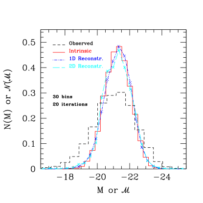
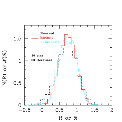
in principle, there are also evolution and K-correction terms which we set to zero. Figure 2 compares ${\cal M}$ with $M$ and ${\cal R}$ with $R$.

Figure 2: Distributions of intrinsic and estimated absolute magnitudes (top panel) and sizes (bottom panel) which result from the differences between true and photo-$z$ shown in the previous Figure.

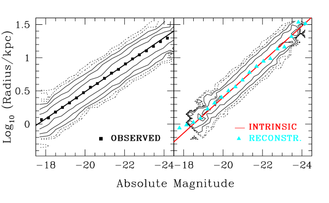
The qualitative nature of the distributions in the two panels are easy to understand. The distribution in ${\cal M}$ is broader than that in $M$, as is the distribution of ${\cal R}$ compared to $R$: photometric redshift errors have broadened both distributions. However, the changes to the estimated absolute magnitude and size are not independent. Assuming an object is closer than it really is makes one infer a fainter luminosity and smaller size than it really has. These correlated changes can have a dramatic effect on the size-luminosity relation, since photo-$z$ errors move each galaxy in the $R-M$ plane left and down or right and up. In general, these motions are not parallel to the principal axis of the true relation, so the mean relation in the photo-$z$ catalog, $\langle{\cal R}|{\cal M}\rangle$, need not be the same as the true relation $\langle R|M\rangle$. In our mock catalog, $\langle{\cal R}|{\cal M}\rangle\propto-0.20\,{\cal M}$, whereas $\langle R|M\rangle\propto-0.27\,M$ (see Figure 3).

Figure 3: Effect of photo-$z$ on the size-luminosity correlation in our mock catalog. In the left panel, contours and solid line show the ${\cal R}-{\cal M}$ relation associated with photo-$z$s, whereas the right panel shows the intrinsic $R-M$ relation. Note the strong bias (shallower slope in panel on left) which results from the fact that the photo-$z$ distance error moves points down and left or up and right on this plot. Squares in left panel show the binned starting guess for the 2d deconvolution algorithm, and triangles in right panel show the result after 20 iterations (equation 13). Convergence to the correct solution is clearly seen.

3 A non-parametric deconvolution-like method

Sheth (2007) shows that to extend Schmidt’s (1968) $V_{\rm max}$ estimator of the luminosity function $\phi(M)$ so that it produces unbiased results in photo-$z$ surveys, it is helpful to think of ${\cal N}({\cal M})$, the number of observed objects with estimated ${\cal M}$, as being a convolution of the true number which have $M$, $N(M)$, with the probability that an object with magnitude $M$ is thought to have magnitude ${\cal M}$. The luminosity function is then estimated by first deconvolving the distribution of ${\cal N}({\cal M})$ to obtain $N(M)$, and then using the fact that $N(M)\equiv\phi(M)\,V_{\rm max}(M)$.

For the same reason, the present problem may be thought of as a two dimensional deconvolution problem (or an $n$-dimensional deconvolution if we were interested in the full manifold, rather than just two-dimensional projections of it). Specifically, let

$$N(M,R)=N(M)\,p(R|M)=V_{\rm max}(M)\,\phi(M)\,p(R|M)$$ (3)

denote the (true) number of galaxies with absolute magnitude $M$ and size $R$ in a magnitude-limited catalog. Here $p(R|M)$ is the probability of having size $R$ when the magnitude is $M$. Similarly, set ${\cal N}({\cal M},{\cal R})={\cal N}({\cal M})~{}p({\cal R}|{\cal M})$. Then

$${\cal N}({\cal M},{\cal R}) = \int{\rm d}M\int{\rm d}R~{}N(M,R)~{}p({\cal M},{\cal R}|M,R)$$ (4)

$$= \int{\rm d}M~{}N[M,{\cal R}-F(M,{\cal M})]~{}p({\cal M}|M),$$

where $F=({\cal M}-M)/5+2\log[(1+\zeta)/(1+z)]$. Our problem is to obtain a reliable estimate of the intrinsic $N(M,R)$ given the photo-$z$ biased ${\cal N}({\cal M},{\cal R})$ and the error distribution $p({\cal M}|M)$. We do this using the deconvolution algorithm proposed by Lucy (1974).

Before we present our algorithm and results, it is worth noting that we could have attempted to invert equation (4) in other ways. Classical naive ‘exact’ inversion methods include matrix-quadrature techniques (reduction of the integral equation to a linear matrix system), polynomial expansion methods, singular function expansion and product integration methods. These typically run into difficulties because the measured data function usually cannot provide sufficient information on the high frequency components of the solution. A standard non-classical technique (Phillips 1962; Twomey 1963; Tikhonov 1963) is the method of regularisation. A “regularisation” parameter is introduced, which balances the size of the residual against the smoothness of the solution, and the problem is turned into one of minimization. However, there is no general strategy for choosing the optimum regularisation parameter; this led Lucy (1974) to formulate his algorithm, and is what has led us to choose his algorithm over these others. One might argue that we are likely to know a fair amount about the expected form of the intrinsic distribution (e.g., luminosity functions are rather smooth, and conditional distributions tend to be bell-shaped), so it may be that these other methods are worth pursuing further. This is the subject of work in progress.

3.1 The deconvolution algorithm

The general two-dimensional problem is that of estimating the frequency distribution $\Psi(\xi^{\prime},\eta^{\prime})$ of the quantities $\xi^{\prime}$ and $\eta^{\prime}$ when the available measures ${x^{\prime}_{1},y^{\prime}_{1};x^{\prime}_{2},y^{\prime}_{2};...,x^{\prime}_{N},y^{\prime}_{N}}$ are a finite sample drawn from an infinite population characterized by:

$$\Phi(x,y)=\int{\rm d}\xi\int{\rm d}\eta~{}\Psi(\xi,\eta)~{}p(x,y|\xi,\eta).$$ (5)

Here $\Phi(x,y)$ is the function accessible to measurement and $p(x,y|\xi,\eta)$ is the conditional probability that $x^{\prime}$ will fall in $[x,x+{\rm d}x]$ when it is known that $\xi^{\prime}\equiv\xi$, and that $y^{\prime}$ will fall in $[y,y+{\rm d}y]$ when $\eta^{\prime}\equiv\eta$. In many cases $\Phi$ and $\Psi$ represent probability density functions, so they obey normalization and non-negativity constraints.

The iterative procedure for generating estimates to $\Psi$ presented in Lucy (1974) is

$$\Psi^{r+1}(\xi,\eta)=\Psi^{r}(\xi,\eta)\int{\rm d}x\int{\rm d}y~{}\frac{\tilde{\Phi}(x,y)}{\Phi^{r}(x,y)}~{}p(x,y|\xi,\eta),$$ (6)

where

$$\Phi^{r}(x,y)=\int{\rm d}\xi\int{\rm d}\eta~{}\Psi^{r}(\xi,\eta)~{}p(x,y|\xi,\eta).$$ (7)

The index $r$ indicates the $r$th iteration in the sequence of estimates, and $\tilde{\Phi}$ is an approximation to $\Phi$ obtained from the observed sample. Convergence is achieved if $\Phi^{r}=\tilde{\Phi}$. The starting approximation $\Psi^{0}(\xi,\eta)$ should be a smooth, non-negative function having the same integrated density as the observed distribution. The extension to $n$-dimensions is obvious, although, if the number of dimensions is large, then performing the multi-dimensional integrations efficiently may become challenging.

The two-dimensional problem simplifies if, as happens in our problem,

$$p(x,y|\xi,\eta) = p(x|\xi)\,p(y|\xi,\eta,x)$$ (8)

$$= p(x|\xi)\,\delta_{\rm D}\Bigl{[}y=\eta-F(x,\xi)\Bigr{]}$$

because the delta function simplifies one of the integrals. The iterative scheme becomes

$$\Psi^{r+1}(\xi,\eta)=\Psi^{r}(\xi,\eta)\int{\rm d}x~{}\frac{\tilde{\Phi}[x,\eta-F(x,\xi)]}{\Phi^{r}[x,\eta-F(x,\xi)]}~{}p(x|\xi)$$ (9)

with

$$\Phi^{r}(x,y)=\int{\rm d}\xi~{}\Psi^{r}[\xi,y+F(x,\xi)]~{}p(x|\xi).$$ (10)

Partial distributions can be easily computed via marginalization from $\Psi^{r+1}$:

$$\Psi^{r+1}(\xi)=\int{\rm d}\eta~{}\Psi^{r+1}(\xi,\eta),$$ (11)

$$\Psi^{r+1}(\eta)=\int{\rm d}\xi~{}\Psi^{r+1}(\xi,\eta).$$ (12)

and

$$\langle\eta|\xi\rangle^{r+1}=\int{\rm d}\eta~{}\eta~{}\frac{\Psi^{r+1}(\eta,\xi)}{\Psi^{r+1}(\xi)}.$$ (13)

The generalization to $n$-dimensions is a straightforward extension of the expressions above, so we do not present explicit expressions. Note that, just as happens in the 2-dimensional case presented here, delta-functions will reduce the $n$-dimensional problem to a simple one-dimensional integral, because the same distance error affects all $n$ quantities.

Figure 4: Reconstruction of the intrinsic $N(M)$ distribution from the distribution of estimated redshifts. Dashed histogram shows the observed absolute magnitude distribution, used as a starting guess. Jagged lines show the reconstructed intrinsic distribution after 20 iteration, using the simpler 1d algorithm (blue) or a 2d iterative scheme (cyan).

Figure 5: Reconstruction of the intrinsic $N(R)$ distribution from the distribution of estimated redshifts. Line styles same as previous Figure.

Figure 6: Examples of reconstructed conditional distributions $p(R|M)$ bins in magnitude of width $\Delta M=0.355$ centred on $M=-22.046,-21.691,-20.982$. Jagged lines show the distributions recovered by the 2d deconvolution algorithm after 20 iterations.

3.2 Results

The formalism outlined above is readily applicable to the size-luminosity correlation if we interpret ($x,y$) as the estimated absolute magnitudes and sizes (${\cal M},{\cal R}$), and ($\xi,\eta$) as the true intrinsic ones, ($M,R$).

Figures 4 and 5 show how well this method recovers the intrinsic distribution of absolute magnitudes and sizes (solid histograms). The broad dashed histograms show the photo-$z$ derived ${\cal M}$ and ${\cal R}$ distributions. These were used as a convenient starting guess in the deconvolution algorithm, although prior knowledge about the expected intrinsic shapes could have been used instead. The reconstruction after 20 iterations is shown by the jagged lines. Of course, we could have chosen to reconstruct $N(M)$ directly from ${\cal N}({\cal M})$, using the 1d deconvolution algorithm outlined in Sheth (2007). This procedure converges in about 5 iterations to the distribution shown by the crosses. Note how well the deconvolved distributions match the intrinsic ones.

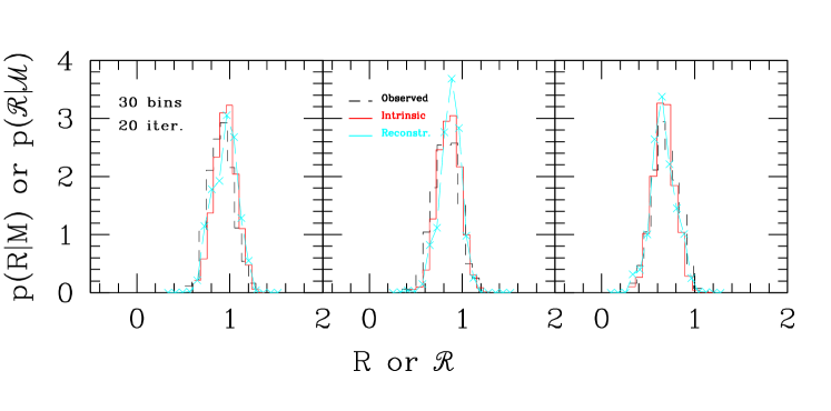
A more stringent test is to check if the conditional distributions, $p(R|M)$, are also well recovered. Figure 6 shows $p(R|M)$ for three bins of width $\Delta M=0.355$ centred at $-22.046$, $-21.691$ and $-20.982$. Clearly, the method works well.

The means of these recovered distributions can be used as an estimate of the recovered size-luminosity relation: $\langle R|M\rangle$. Recall we had noted that this relation was rather strongly biased because use of the photo-$z$ distance estimate means that the error in the size is correlated with that on the luminosity. The squares in the left hand panel of Figure 3 show the starting guess for our algorithm, and the triangles in the right hand panel show the reconstructed relation obtained from the deconvolution procedure — it is in excellent agreement with the true one.

4 A maximum-likelihood method

Sheth (2007) describes an algorithm which produces a maximum-likelihood estimate of the luminosity function from magnitude limited photo-$z$ datasets. It is straightforward to extend that analysis to the present case, in which the quantity of interest is not just the distribution of luminosities, but the joint distribution of luminosity and other observed physical parameters.

Let ${{\mbox{\boldmath$\cal M$}}}_{i}$ denote the vector of physical quantities for galaxy $i$ estimated using the photometric redshift $\zeta_{i}$ when computing distances, and let ${\cal N}({{\mbox{\boldmath$\cal M$}}}_{i},\zeta_{i}|{{\mbox{\boldmath$a$}}})$ denote the number of galaxies in a magnitude limited catalog that have estimated redshifts $\zeta_{i}$ and estimated luminosities, sizes, etc., ${{\mbox{\boldmath$\cal M$}}}_{i}$, when the model for the intrinsic joint distribution of physical quantities is specified by the parameters $a$. Then, dropping the understood $i$-index dependence,

$${\cal N}({{\mbox{\boldmath$\cal M$}}},\zeta|{{\mbox{\boldmath$a$}}})=\int{\rm d}z{{\rm d}V_{\rm c}\over{\rm d}z}\,\phi({{\mbox{\boldmath$M$}}}|{{\mbox{\boldmath$a$}}})\,p\Bigl{(}\zeta|z,m({{\mbox{\boldmath$\cal M$}}},\zeta)\Bigr{)},$$ (14)

where $p(\zeta|z,m)$ is the photo-$z$ redshift error distribution, and $\phi({{\mbox{\boldmath$M$}}}|{{\mbox{\boldmath$a$}}})$ denotes the true joint distribution of physical quantities, but evaluated at values which account for the fact that the same photo-$z$ error which affects the absolute magnitudes affects the other observables. E.g., in the size-luminosity relation we have been considering,

$${{\mbox{\boldmath$\cal M$}}}=({\cal M},{\cal R})\qquad{\rm and}\qquad{{\mbox{\boldmath$M$}}}=(M,R),$$ (15)

where

$$M = {\cal M}-5\log_{10}[D_{\rm L}(z)/D_{\rm L}(\zeta)]$$ (16)

$$R = {\cal R}+\log_{10}[D_{\rm A}(z)/D_{\rm A}(\zeta)].$$ (17)

The factor of $m$ is the apparent magnitude associated with photo-$z$ redshift $\zeta$ and absolute magnitude ${\cal M}$; of course, $m$ is the same for true redshift $z$ and absolute magnitude $M$.

The predicted number of objects with photometric redshift $\zeta$ when the model has parameters $a$ is

$${\cal N}(\zeta|{{\mbox{\boldmath$a$}}})=\int{\rm d}{{\mbox{\boldmath$\cal M$}}}\,{\cal N}({{\mbox{\boldmath$\cal M$}}},\zeta|{{\mbox{\boldmath$a$}}}).$$ (18)

If the redshift-error distribution is independent of $m$, then

$${\cal N}(\zeta|{{\mbox{\boldmath$a$}}}) = \int{\rm d}z\,({\rm d}V_{\rm c}/{\rm d}z)\,S(z,{{\mbox{\boldmath$a$}}})\,p(\zeta|z)$$ (19)

$$\equiv \int{\rm d}z\,N(z|{{\mbox{\boldmath$a$}}})\,p(\zeta|z),$$

where

$$S(z,{{\mbox{\boldmath$a$}}})=\int_{M_{\rm max}(z)}^{M_{\rm min}(z)}{\rm d}M\,\phi(M).$$ (20)

This shows that ${\cal N}(\zeta|{{\mbox{\boldmath$a$}}})$ is just the convolution of the intrinsic redshift distribution (in a flux-limited catalog) with the redshift-error distribution.

The expressions above generalize those given in Sheth (2007), where ${{\mbox{\boldmath$\cal M$}}}={\cal M}$ and ${{\mbox{\boldmath$M$}}}=M$, with $M$ given by equation (16). Hence, by analogy to when the distances are known accurately, the likelihood to be maximized is (reintroducing the index $i$)

$${\cal L}({{\mbox{\boldmath$a$}}})=\prod_{i}\,p_{i},\qquad{\rm where}\qquad p_{i}={{\cal N}({{\mbox{\boldmath$\cal M$}}}_{i},\zeta_{i}|{{\mbox{\boldmath$a$}}})\over{\cal N}(\zeta_{i}|{{\mbox{\boldmath$a$}}})}.$$ (21)

The analysis in Sheth (2007) can now be followed to show analytically that this is indeed the appropriate expression for the likelihood, so we do not reproduce it here.

5 Discussion and future work

We presented two algorithms for reconstructing the intrinsic correlations between distance-dependent quantities in apparent magnitude limited photometric redshift datasets. One was a generalization of the non-parametric $V_{\rm max}$ method (Section 3), and the other used a maximum-likelihood approach (Section 4).

Both our reconstruction methods assume that the distribution of photo-$z$ errors is known accurately. In practice, this means that spectroscopic redshifts are available for a subset of the data. The question then arises as to whether or not the number of spectra which must be taken to specify the error distribution reliably is sufficient to also provide a reliable (spectroscopic!) estimate of these scaling relations. If so, what is the basis for deciding that it is worth reconstructing these relations from the photo-$z$ data? This is the subject of work in progress, although the methods presented in this paper assume that such reconstructions will indeed be necessary. E.g., if the spectra are not simply a random subset of the magnitude limited photometric sample, then it may be difficult to quantify and so correct for the selection effects associated with the spectroscopic subset.

We used the size-luminosity relation in a mock catalog which had realistic choices for the correlation to illustrate the biases which are present and must be corrected if photometric redshift datasets are to provide reliable estimates of galaxy scaling relations (Figures 2 and 3). We showed that our iterative deconvolution scheme provides a simple and reliable correction of this bias (Figures 3–6). Note that although we have illustrated our methods using a 2-dimensional distribution, the extension to $n$-correlated variables is trivial.

Because our algorithm permits the accurate measurement of many scaling relations for which spectra were previously thought to be necessary (e.g. the color-magnitude relation, the size-surface brightness relation, the Photometric Fundamental Plane), we hope that our work will permit photometric redshift surveys to provide more stringent constraints on galaxy formation models at a fraction of the cost of spectroscopic surveys.

Our results may have other applications. For example, Bernardi (2007) has highlighted a bias associated with the correlation between stellar velocity dispersion $\sigma$ and luminosity $L$ which arises if the distance indicator used to estimate $L$ is correlated with $\sigma$ (as may happen in the local Universe, where peculiar velocities make spectroscopic redshifts unreliable distance estimators). It may be that the methods presented here would allow an accurate reconstruction of the true relation from the biased one. This is the subject of on-going work.

References

- (1)
- Bernardi (2007) Bernardi M., 2007, ApJ, 660, 267
- Bernardi et al. (2003) Bernardi M., et al., 2003, AJ, 125, 1849
- Chen et al. (2003) Chen H.-W., et al. 2003, ApJ, 586, 745
- Lucy (1974) Lucy L. B., 1974, AJ, 79, 745
- Phillips (1962) Phillips D. L., 1962, J. Ass. Comput. Mach. 9, 84
- Schmidt (1968) Schmidt M., 1968, ApJ, 151, 393
- Sheth (2007) Sheth R. K., 2007, MNRAS, 378, 709
- Subbarao et al. (1996) Subbarao M. U., Connolly A. J., Szalay A. S., & Koo D. C., 1996, AJ, 112, 929
- Tikhonov (1963) Tikhonov A. N., 1963, Sov. Maths.–Dokl. 4, 1035
- Twomey (1963) Twomey S., 1963, J. Ass. Comput. Mach. 10, 97