Alfvén QPOs in Magnetars

Abstract

We investigate torsional Alfvén oscillations of relativistic stars with a global dipole magnetic field, via two-dimensional numerical simulations. We find that a) there exist two families of quasi-periodic oscillations (QPOs) with harmonics at integer multiples of the fundamental frequency, b) the lower-frequency QPO is related to the region of closed field lines, near the equator, while the higher-frequency QPO is generated near the magnetic axis, c) the QPOs are long-lived, d) for the chosen form of dipolar magnetic field, the frequency ratio of the lower to upper fundamental QPOs is $\sim 0.6$, independent of the equilibrium model or of the strength of the magnetic field, and e) within a representative sample of equations of state and of various magnetar masses, the Alfvén QPO frequencies are given by accurate empirical relations that depend only on the compactness of the star and on the magnetic field strength. The lower and upper QPOs can be interpreted as corresponding to the edges or turning points of an Alfvén continuum, according to the model proposed by Levin (2007). Several of the low-frequency QPOs observed in the X-ray tail of SGR 1806-20 can readily be identified with the Alfvén QPOs we compute. In particular, one could identify the 18Hz and 30Hz observed frequencies with the fundamental lower and upper QPOs, correspondingly, while the observed frequencies of 92Hz and 150Hz are then integer multiples of the fundamental upper QPO frequency (three times and five times, correspondingly). With this identification, we obtain an upper limit on the strength of magnetic field of SGR 1806-20 (if is dominated by a dipolar component) between $\sim 3$ and $7\times 10^{15}$G. Furthermore, we show that an identification of the observed frequency of 26Hz with the frequency of the fundamental torsional $\ell=2$ oscillation of the magnetar’s crust is compatible with a magnetar mass of about $1.4$ to 1.6$M_{\odot}$ and an EOS that is very stiff (if the magnetic field strength is near its upper limit) or moderately stiff (for lower values of the magnetic field).

1 Introduction

The phenomenon of Soft Gamma Repeaters (SGRs) may allow us in the near future to determine fundamental properties of strongly magnetized, compact stars. Already, there exist at least two sources in which quasi-periodic oscillations (QPOs) have been observed in their X-ray tail, following the initial discovery by Israel et al. (2005), see Watts & Strohmayer (2006) for a recent review. The frequency of many of these oscillations is similar to what one would expect for torsional modes of the solid crust of a compact star. This observation is in support of the proposal that SGRs are magnetars (compact objects with very strong magnetic fields) (Duncan & Thompson, 1992). During an SGR event, torsional oscillations in the solid crust of the star could be excited (Duncan, 1998), leading to the observed frequencies in the X-ray tail. However, not all of the observed frequencies fit the above picture. For example, the three lowest observed frequencies for SGR 1806-20 are 18, 26, 30Hz. Only one of these could be the fundamental, $\ell=2,m=0$ torsional frequency of the crust, as the first overtone has a much higher frequency. Levin (2006) stressed the importance of crust-core coupling by a global magnetic field and of the existence of an Alfvén continuum, while Glampedakis et al. (2006) considered model with simplified geometry, in which Alfvén oscillations form a discrete spectrum of normal modes, that could be associated with the observed low-frequency QPOS. In Levin (2007), the existence of a continuum was stressed further and it was shown that the edges or turning points of the continuum can yield long-lived QPOs. In addition, numerical simulations showed that drifting QPOs within the continuum become amplified near the frequencies of the crustal normal modes. Within this model, Levin suggested a likely identification of the 18Hz QPO in SGR 1806-20 with the lowest frequency of the MHD continuum or its first overtone. The above results were obtained in toy models with simplified geometry and Newtonian gravity.

In this Letter, we perform two-dimensional numerical simulations of linearized Alfvén oscillations in magnetars. Our model improves on the previously considered toy models in various ways: relativistic gravity is assumed, various realistic equations of state (EOS) are considered and a consistent dipolar magnetic field is constructed. We do not consider the presence of a solid crust, but only examine the response of the ideal magnetofluid to a chosen initial perturbation.

Spherical stars have generally two type of oscillations, spheroidal with polar parity and toroidal with axial parity. The observed QPOs in SGR X-ray tails may originate from toroidal oscillations, since these could be excited more easily than poloidal oscillations, because they do not involve density variations. In Newtonian theory, there have been several investigations of torsional oscillations in the crust region of neutron stars (see e.g., Lee (2007) for reference). On the other hand, only few studies have taken general relativity into account (Messios et al., 2001; Sotani et al., 2007a, b; Samuelsson & Andersson, 2007; Vavoulidis et al., 2007).

SGRs produce giant flares with peak luminosities of $10^{44}$ – $10^{46}$ erg/s, which display a decaying tail for several hundred seconds. Up to now, three giant flares have been detected, SGR 0526-66 in 1979, SGR 1900+14 in 1998, and SGR 1806-20 in 2004. The timing analysis of the latter two events revealed several QPOs in the decaying tail, whose frequencies are approximately 18, 26, 30, 92, 150, 625, and 1840 Hz for SGR 1806-20, and 28, 53, 84, and 155 Hz for SGR 1900+14, see Watts & Strohmayer (2006).

In Sotani et al. (2007a) (hereafter Paper I), it was suggested that some of the observational data of SGRs could agree with the crustal torsional oscillations, if, e.g., frequencies lower than 155 Hz are identified with the fundamental oscillations of different harmonic index $\ell$, while higher frequencies are identified with overtones. However, in Paper I and above, it will be quite challenging to identify all observed QPO frequencies with only crustal torsional oscillations. For example, it is difficult to explain all of the frequencies of 18, 26 and 30 Hz for SGR 1806-20 with crustal models, because the actual spacing of torsional oscillations of the crust is larger than the difference between these two frequencies. Similarly, the spacing between the 625Hz and a possible 720Hz QPO in SGR 1806-20 may be too small to be explained by consecutive overtones of crustal torsional oscillations.

One can notice, however, that the frequencies of 30, 92 and 150 Hz in SGR 1806-20 are in near integer ratios. As we will show below, the numerical results presented in this Letter are compatible with this observation, as we find two families of QPOs (corresponding to the edges or turning points of a continuum) with harmonics at near integer multiples. Furthermore, our results are compatible with the ratio of 0.6 between the 18 and 30Hz frequencies, if these are identified, as we suggest, with the edges (or turning points) of the Alfvén continuum. With this identification, we can set an upper limit to the dipole magnetic field of $\sim 3$ to $~{}7\times 10^{15}$G. If the drifting QPOs of the continuum are amplified at the fundamental frequency of the crust, and the latter is assumed to be the observed 26Hz for SGR 1806-20, then our results are compatible with a magnetar mass of about $1.4$ to 1.6$M_{\odot}$ and an EOS that is very stiff (if the magnetic field strength is near its upper limit) or moderately stiff (for lower values of the magnetic field).

Unless otherwise noted, we adopt units of $c=G=1$, where $c$ and $G$ denote the speed of light and the gravitational constant, respectively, while the metric signature is $(-,+,+,+)$.

2 Numerical Setup

The general-relativistic equilibrium stellar model is assumed to be spherically symmetric and static, i.e. a solution of the well-known TOV equations for and perfect fluid and metric described the line element

$$ds^{2}=-e^{2\Phi(r)}dt^{2}+e^{2\Lambda(r)}dr^{2}+r^{2}(d\theta^{2}+\sin^{2}\theta d\phi^{2}).$$ (1)

We neglect the influence of the magnetic field on the structure of the star, since the magnetic field energy, ${\cal E_{M}}$, is orders of magnitudes smaller than the gravitational binding energy, ${\cal E_{G}}$, for magnetic field strengths considered realistic for magnetars, ${\cal E_{M}}/{\cal E_{G}}\approx 10^{-4}(B/(10^{16}{\rm G}))^{2}$. For simplicity, we assume that the magnetic field is a pure dipole (toroidal magnetic fields will be treated elsewhere, see Sotani et al. (2007c). Details on the numerical method for constructing the magnetic field, as well as representative figure of the magnetic field lines, can be found in Paper I.

MHD oscillations of the above equilibrium model are described by the linearized equations of motion and the magnetic induction equations, presented in detail in Papers I and II (we neglect perturbations in the spacetime metric, as these couple weakly to toroidal modes in a spherically symmetric background). The perturbative equations presented in Papers I and II can readily be converted from an eigenvalue problem to the form of a two-dimensional time-evolution problem, by defining a displacement ${\cal Y}(t,r,\theta)$ due to the toroidal motion (the coefficient of shear viscosity is set to $\mu=0$, as we neglect the presence of a solid crust in the present work). The contravariant coordinate component of the perturbed four-velocity, $\delta u^{\phi}$, is then related to time derivative of ${\cal Y}$ through

$$\delta u^{\phi}=e^{-\Phi}\partial_{t}{\cal Y}(t,r,\theta).$$ (2)

The two-dimensional evolution equation for ${\cal Y}(t,r,\theta)$ is

$${\cal A}_{tt}\frac{\partial^{2}{\cal Y}}{\partial t^{2}} = {\cal A}_{20}\frac{\partial^{2}{\cal Y}}{\partial r^{2}}+{\cal A}_{11}\frac{\partial^{2}{\cal Y}}{\partial r\partial\theta}+{\cal A}_{02}\frac{\partial^{2}{\cal Y}}{\partial\theta^{2}}$$ (3)

$$+ {\cal A}_{10}\frac{\partial{\cal Y}}{\partial r}+{\cal A}_{01}\frac{\partial{\cal Y}}{\partial\theta}+\varepsilon_{D}{\cal D}_{4}{\cal Y},$$

where ${\cal A}_{tt}$, ${\cal A}_{20}$, ${\cal A}_{11}$, ${\cal A}_{02}$, ${\cal A}_{10}$, and ${\cal A}_{01}$ are functions of $r$ and $\theta$, given by

$${\cal A}_{tt} = \left[\epsilon+p+\frac{{a_{1}}^{2}}{\pi r^{4}}\cos^{2}\theta+\frac{{{a_{1}}^{\prime}}^{2}}{4\pi r^{2}}e^{-2\Lambda}\sin^{2}\theta\right]e^{-2(\Phi-\Lambda)},$$ (4)

$${\cal A}_{20} = \frac{{a_{1}}^{2}}{\pi r^{4}}\cos^{2}\theta,$$ (5)

$${\cal A}_{11} = -\frac{a_{1}{a_{1}}^{\prime}}{\pi r^{4}}\sin\theta\cos\theta,$$ (6)

$${\cal A}_{02} = \frac{{{a_{1}}^{\prime}}^{2}}{4\pi r^{4}}\sin^{2}\theta,$$ (7)

$${\cal A}_{10} = \left(\Phi^{\prime}-\Lambda^{\prime}\right)\frac{{a_{1}}^{2}}{\pi r^{4}}\cos^{2}\theta+\frac{a_{1}{a_{1}}^{\prime}}{2\pi r^{4}}\sin^{2}\theta,$$ (8)

$${\cal A}_{01} = \left[\frac{a_{1}}{\pi r^{4}}\left(2\pi j_{1}-\frac{a_{1}}{r^{2}}\right)e^{2\Lambda}+\frac{3{{a_{1}}^{\prime}}^{2}}{4\pi r^{4}}\right]\sin\theta\cos\theta,$$ (9)

and where $a_{1}(r)$ and $j_{1}(r)$ are the radial components of the electromagnetic four-potential and the four-current, respectively. In the above equations, a prime denotes a partial derivative with respect to the radial coordinate.

In our numerical scheme, we employ the 2nd-order, iterative Crank-Nicholson scheme. A numerical instability, which sets in after many oscillations, was treated by adding a 4th-order Kreiss-Oliger dissipation term (Kreiss & Oliger, 1973), shown as $\varepsilon_{D}{\cal D}_{4}{\cal Y}$ in Equation (3) above. We experimented with various values of the dissipation coefficient $\varepsilon_{D}$ and found the evolution to be stable for values as small as a few times $10^{-5}$. We verified that in this limit, the solution becomes independent of the strength of the numerical dissipation, as the ${\cal D}_{4}$ Kreiss-Oliger dissipation operator introduces an error of higher order than the 2nd-order iterative Crank-Nicholson scheme. The numerical grid we use is equidistant, covering only the interior of the star, with (typically) 50 radial zones and 40 angular zones (we also compared our results to simulations with 100x80 points). The boundary conditions are: (a) ${\cal Y}=0$ at $r=0$ (regularity), (b) ${\cal Y}_{,r}=0$ at $r=R$ (vanishing traction) (c) ${\cal Y}_{,\theta}=0$ at $\theta=0$ (axisymmetry) and (d) ${\cal Y}=0$ at $\theta=\pi/2$ (equatorial plane symmetry of the $\ell=2$ initial data). We obtain the same results if you use a grid that extends to $\theta=\pi$. We have also evolved initial data with $\ell=3$, for which the appropriate boundary condition at $\theta=\pi/2$ is ${\cal Y}_{,\theta}=0$.

3 Alfvén QPOs

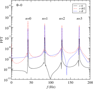
Figure 1: FFT of the MHD oscillations at $\theta\sim 0$ (magnetic axis). Three lines in each figure correspond to different radial positions $r\sim 0$, $R/2$, and $R$). A fundamental ($n=0$) QPO and several overtones (nearly integer multiples) are clearly present.

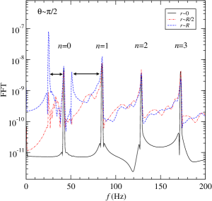
Figure 2: Same as Fig. 1, but at $\theta\sim\pi/2$ (magnetic equator). A second family of QPOs is present. Arrows indicate several continuous parts, of which only the first is distinct from the others, which partially overlap.

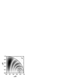
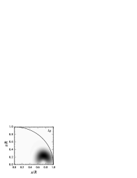
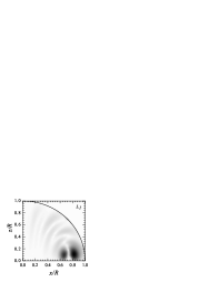
Figure 3: Distribution of effective amplitude of several Alfvén QPOs (see text for details). The grayscale map varies from white (zero amplitude) to black (maximum amplitude).

As a fist equilibrium model, we examined a polytropic stellar model with $\Gamma=2$, whose mass and radius are $M=1.4M_{\odot}$ and $R=14.16$ km, respectively, with a dipole magnetic field strength of $B\equiv B_{\mu}=4\times 10^{15}$ G, where $B_{\mu}$ is a typical strength. As initial data, we use the numerical eigenfunction of the $\ell=2,m=0$ fundamental mode, for the truncated system presented in Paper II. The grid size is $100\times 80$ and $\varepsilon_{D}=10^{-3}$, while the total simulation time is 2s. By computing the FFT of $\partial_{t}{\cal Y}$ (which is proportional to $\delta u^{\phi}$) at various points inside the star, we obtain the following results: Examining the FFT at three different radial locations ($r\sim 0,R/2,R$) at $\theta\sim 0$ (magnetic axis), Fig. 1, we observe a number of narrow frequency peaks. The strength of the peaks is several orders of magnitude larger than the FFT continuum. The overtones ($n>0$) are nearly integer multiples of the fundamental frequency ($n=0)$. The corresponding FFTs at the same radial points, but at $\theta\sim\pi/2$ (magnetic equator) are shown in Fig. 2, where, in addition to the family of frequency peaks observed in Fig. 1, one can also observe a second family of frequency peaks, mainly at $r\sim R$, for which the fundamental frequency is at a ratio of 0.6 with respect to the fundamental frequency in Fig. 1. The fundamental frequency of this family, as well as the first overtone (again an integer multiple) are clearly visible, while the other overtones seem to be buried inside a continuum of other frequencies.

Using Levin’s toy model for the Alfvén continuum in magnetars, the above numerical results can be interpreted as follows: The fundamental frequency peaks of the two families are QPOs generated by the edges or turning points of an Alfvén continuum (henceforth we call these two frequencies as the fundamental lower and upper QPOs and denote them as $L_{0}$ and $U_{0}$). We denote the overtones (which are nearly integer multiples) as $L_{n}$ and $U_{n}$, where $n>0$. For the chosen form of the magnetic field, the extent of the first continuum, between the fundamental $L_{0}$ and $U_{0}$ QPOs is at lower frequencies than the continuous frequency intervals corresponding to the overtones, which all overlap partially.

Because of the Alfvén continuum, the phase of the oscillations at the QPO frequencies is not constant, but varies throughout the star. Since the magnetic field is axisymmetric, the axis is both a turning point and edge of the continuum. Near the magnetic axis, the background magnetic field varies slowly, which allows for the upper QPOs to remain nearly coherent for a large number of oscillations. Since $\delta u^{\phi}$ is only a coordinate component, we also obtained FFTs of $r\sin\theta\partial_{t}{\cal Y}$ (which is proportional to the physical velocity in a unit basis) at all grid points. In two-dimensional simulations of fluid modes in non-magnetized stars, it has been shown that the amplitude of the FFT of physical variables at every point in the numerical grid, at a chosen normal mode frequency, is correlated to the shape of the eigenfunction of a given mode (Stergioulas et al., 2004). Similarly, we use the magnitude of the FFT of $r\sin\theta\partial_{t}{\cal Y}$ at every point in the grid to define an effective amplitude for each QPO (which, of course, will be time-varying, due to the absorption of individual modes in the continuum). In Fig. 3, we show the effective amplitude of the fundamental upper QPO, $U_{0}$ and its first overtone $U_{1}$ as well as for the corresponding lower QPOs $L_{0}$ and $L_{1}$, obtained after a simulation with a $50\times 40$ grid, $\varepsilon_{D}=2\times 10^{-5}$ and a duration of 2.1s.

The effective amplitude for $U_{0}$ has a maximum near the magnetic axis, while there are also nodal lines along certain magnetic field lines. For the overtone, $U_{1}$, there exists an additional nodal line, starting perpendicular near the magnetic axis, which divides the region of maximum amplitude near the magnetic axis roughly in half. Similarly (not shown here), each successive overtone corresponds to an additional “horizontal” nodal line, dividing the region of maximum amplitude near the magnetic axis into roughly equidistant parts. This agrees well with the fact that the frequencies of the overtones are nearly integer multiples of the fundamental frequency.

The effective amplitude of the fundamental lower QPO, $L_{0}$, is practically limited to a region that is only somewhat larger than the region of closed magnetic field lines inside the star. For the first overtone $L_{1}$, a nodal line divides the region of maximum amplitude into two parts.

In Fig. 4 we show the evolution of $\partial_{t}{\cal Y}$ at the location inside the star where the effective amplitude of the fundamental upper QPO, $U_{0}$ attains its maximum value. It is evident that the QPO is long-lived, since the amplitude of the oscillations barely diminishes with time.

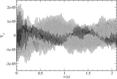
Figure 4: Time evolution of $\partial_{t}{\cal Y}$ at the location inside the star where the effective amplitude of the fundamental upper QPO, $U_{0}$ attains its maximum value. The amplitude of the oscillations barely diminish with time

Table 1: Frequencies of lower and upper Alfvén QPOs and their ratios, for a representative sample of equilibrium models, constructed with various EOSs and masses and for a magnetic field strength of $B=B_{\mu}$ (see text for details).

Model	M/R	$f_{L_{0}}$ (Hz)	$f_{U_{0}}$ (Hz)	ratio	$f_{L_{1}}$ (Hz)	$f_{U_{1}}$ (Hz)	ratio	$f_{U_{2}}$ (Hz)
A+DH14	0.218	15.4	25.0	0.616	30.7	49.4	0.621	74.4
A+DH16	0.264	11.7	18.3	0.639	23.5	35.7	0.658	54.0
WFF3+DH14	0.191	17.9	29.8	0.601	36.2	59.2	0.611	89.8
WFF3+DH18	0.265	11.7	18.0	0.650	23.5	35.5	0.662	53.3
APR+DH14	0.171	20.4	34.1	0.598	41.3	68.6	0.602	104.6
APR+DH20	0.248	12.8	20.6	0.621	26.0	40.3	0.645	61.0
L+DH14	0.141	23.7	40.8	0.581	47.5	81.6	0.582	123.8
L+DH20	0.199	16.4	27.8	0.590	33.1	54.7	0.605	82.6

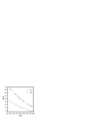
Figure 5: Quadratic fits in terms of the compactness of the star, $M/R$, of the lower and upper fundamental Alfvén QPO frequencies, obtained for a representative sample of equilibrium models with various EOSs and masses. The magnetic field was set to $B=B_{\mu}$.

4 Realistic EOS and Empirical Relations

We have obtained the lower and upper Alfvén QPO frequencies for a representative sample of magnetar models with realistic (tabulated) EOSs and various masses. These equilibrium models and their detailed properties have already been presented in Paper I. In Table 1 we summarize our numerical results for $B=B_{\mu}$, for a somewhat smaller sample of models, than the one considered in Paper I. As in the case of the polytropic model of Sec. 3, the overtones are nearly integer multiples of the fundamental frequency

$$f_{L_{n}} \simeq (n+1)f_{L_{0}},$$ (10)

$$f_{U_{n}} \simeq (n+1)f_{U_{0}},$$ (11)

with an accuracy on the order of 1% or better. In addition, the ratio of the lower to upper QPO frequencies (also shown in Table 1) roughly agrees with the value of 0.6 for the polytropic model. A quadratic fit in terms of $M/R$ gives:

$$\frac{f_{L_{0}}}{f_{U_{0}}}\simeq 0.62\left[1-1.08\left(\frac{M}{R}\right)+4.52\left(\frac{M}{R}\right)^{2}\right],$$ (12)

with an accuracy of better than $2\%$. Similarly, a quadratic fit for the ratio of the lower to upper first overtone frequencies yields

$$\frac{f_{L_{1}}}{f_{U_{1}}}\simeq 0.58\left[1-0.54\left(\frac{M}{R}\right)+3.88\left(\frac{M}{R}\right)^{2}\right],$$ (13)

with a similar accuracy.

We find that the frequencies of the Alfvén QPOs scale linearly with the strength of the magnetic field (with an accuracy on the order of 1% or better) at least for magnetic field strengths on the order of $B_{\mu}$.

Within the representative sample of the equilibrium models we display in Table 1, the frequencies of all lower and upper Alfvén QPOs (with $n=0,1,2,...$) are given by the following two empirical relations

$$f_{L_{n}}({\rm Hz}) \simeq 48.9(n+1)\left[1-4.51\left(\frac{M}{R}\right)+6.18\left(\frac{M}{R}\right)^{2}\right]$$ (14)

$$\times\left(\frac{B}{4\times 10^{15}{\rm G}}\right),$$

$$f_{U_{n}}({\rm Hz}) \simeq 86.1(n+1)\left[1-4.58\left(\frac{M}{R}\right)+6.06\left(\frac{M}{R}\right)^{2}\right]$$ (15)

$$\times\left(\frac{B}{4\times 10^{15}{\rm G}}\right),$$

with an accuracy of less than about 4%. The quadratic fits in terms of $M/R$, for $B=B_{\mu}$ is shown in Fig. 5. We emphasize that in all of the above relations, the ratio $M/R$ is dimensionless, in gravitational units ($c=G=1$). To restore units, it has to be replaced by $GM/Rc^{2}$.

5 CONSTRAINTS ON MAGNETIC FIELD STRENGTH AND EOS

Several of the low-frequency QPOs observed in the X-ray tail of SGR 1806-20 can readily be identified with the Alfvén QPOs we compute. In particular, one could identify the 18Hz and 30Hz observed frequencies with the fundamental lower and upper QPOs, correspondingly, while the observed frequencies of 92Hz and 150Hz would then be integer multiples of the fundamental upper QPO frequency (three times and five times, correspondingly). With this identification, our empirical relations Eqs. (14) and (15) constrain the magnetic field strength of SGR 1806-20 (if is dominated by a dipolar component) to be between $~{}3\times 10^{15}$G and $~{}7\times 10^{15}$G. Furthermore, an identification of the observed frequency of 26Hz with the frequency of the fundamental torsional $\ell=2$ oscillation of the magnetar’s crust (Eq. (79) of Paper I) implies a very stiff equation of state and a mass of about 1.4 to 1.6$M_{\odot}$. For example, for the $1.4M_{\odot}$ model constructed with EOS L+DH, one obtains the following frequencies: ${}_{2}t_{0}=25.8$Hz, $f_{L_{0}}=17.5$Hz, $f_{U_{0}}=30.0$Hz, $f_{U_{3}}=90.1$Hz and $f_{U_{5}}=150.2$Hz, for $B=2.94\times 10^{15}$ G.

Alternatively, one could also identify the 18Hz and 30Hz observed frequencies with overtones (which are also at a near 0.6 ratio). In this case, the strength of the magnetic field derived above is only an upper limit and the actual magnetic field may be weaker. Then, if one assumes that the observed frequency of 26Hz is due to the fundamental $\ell=2$ crust mode for a weak magnetic field, our numerical data agree best with a  1.4$M_{\odot}$ model constructed with an EOS of moderate stiffness. For example, for the 1.4$M_{\odot}$ model constructed with the APR+DH EOS one obtains ${}_{2}t_{0}=25.9$Hz, $f_{L_{1}}=17.7$Hz, $f_{U_{1}}=30.0$Hz, $f_{U_{5}}=90.1$Hz and $f_{U_{9}}=150.1$Hz, for $B=1.77\times 10^{15}$ G.

6 Discussion

We have already verified that our main QPO frequencies agree with frequencies obtained with an independent, fully nonlinear numerical code (Cerdá-Durán et al., 2007), for the same initial model. We caution, however, that we have not yet considered the crust-core interaction, different magnetic field topologies or the coupling to the exterior magnetosphere. These effects have to be taken into account and already Sotani et al. (2007c), find that the observed QPOs could lead to constraints on the magnetic field topology. To complete the picture, a three-dimensional numerical simulation, that includes a proper coupling of the crust to the MHD interior and to the exterior magnetosphere will be required and our current results provide a good starting point. Extensive details of our computations will be presented in Sotani et al. (2007d).

References

- Cerdá-Durán et al. (2007) Cerdá-Durán P., Sotani H., Stergioulas N., Font J.A., 2007, in preparation
- Duncan & Thompson (1992) Duncan R.C., Thompson C., 1992, ApJ, 392, L9
- Duncan (1998) Duncan R.C.,1998, ApJ, 1998, 498, L45
- Glampedakis et al. (2006) Glampedakis K., Samuelsson L., Andersson N., 2006, MNRAS, 371, L74
- Israel et al. (2005) Israel G. et al., 2005, ApJ, 628, L53
- Kreiss & Oliger (1973) Kreiss H.-O., Oliger J., 1973, Methods for the approximate solution of time dependent problems, GARP Publications Series 10
- Lee (2007) Lee U., 2007, MNRAS, 374, 1015
- Levin (2006) Levin Y., 2006, MNRAS, 368, L35
- Levin (2007) Levin Y., 2007, MNRAS, 377, 159
- Messios et al. (2001) Messios N., Papadopoulos D.B., Stergioulas N., 2001, MNRAS, 328, 1161
- Samuelsson & Andersson (2007) Samuelsson L., Andersson N., 2007, MNRAS, 374, 256
- Sotani et al. (2007a) Sotani H., Kokkotas K.D., Stergioulas N., 2007a, MNRAS, 375, 261 (Paper I)
- Sotani et al. (2007b) Sotani H., Kokkotas K.D., Stergioulas N., Vavoulidis M., 2007b, preprint (astro-ph/0611666) (Paper II)
- Sotani et al. (2007c) Sotani H., Colaiuda A., Kokkotas K.D., 2007c, preprint (gr-qc/0711.1518)
- Sotani et al. (2007d) Sotani H., Kokkotas K.D., Stergioulas N., 2007d, in preparation
- Stergioulas et al. (2004) Stergioulas N., Apostolatos T.A., Font J.A., 2004, MNRAS, 352, 1089
- Vavoulidis et al. (2007) Vavoulidis M., Stavridis A., Kokkotas K.D., Beyer H., 2007, MNRAS, 377, 1553
- Watts & Strohmayer (2006) Watts A.L., Strohmayer T.E., 2006, Advances in Space Research, in press (astro-ph/0612252)