Fractal and Multifractal Scaling of Electrical Conduction in Random Resistor Networks
S. Redner

Article Outline

Glossary
I. Definition of the Subject
II. Introduction to Current Flows
III. Solving Resistor Networks
III.1 Fourier Transform
III.2 Direct Matrix Solution
III.3 Potts Model Connection
III.4 $\Delta$-Y and Y-$\Delta$ Transforms
III.5 Effective Medium Theory
IV. Conduction Near the Percolation Threshold
IV.1 Scaling Behavior
IV.2 Conductance Exponent
V. Voltage Distribution of Random Resistor Networks
V.1 Multifractal Scaling
V.2 Maximum Voltage
VI. Random Walks and Resistor Networks
VI.1 The Basic Relation
VI.2 Network Resistance and Pólya’s Theorem
VII. Future Directions
VIII. Bibliography

Glossary

conductance ($G$): the relation between the current $I$ in an electrical network and the applied voltage $V$: $I=GV$.

conductance exponent ($t$): the relation between the conductance $G$ and the resistor (or conductor) concentration $p$ near the percolation threshold: $G\sim(p-p_{c})^{t}$.

effective medium theory (EMT): a theory to calculate the conductance of a heterogeneous system that is based on a homogenization procedure.

fractal: a geometrical object that is invariant at any scale of magnification or reduction.

multifractal: a generalization of a fractal in which different subsets of an object have different scaling behaviors.

percolation: connectivity of a random porous network.

percolation threshold $p_{c}$: the transition between a connected and disconnected network as the density of links is varied.

random resistor network: a percolation network in which the connections consist of electrical resistors that are present with probability $p$ and absent with probability $1-p$.

I Definition of the Subject

Consider an arbitrary network of nodes connected by links, each of which is a resistor with a specified electrical resistance. Suppose that this network is connected to the leads of a battery. Two natural scenarios are: (a) the “bus-bar geometry” (Fig. 1), in which the network is connected to two parallel lines (in two dimensions), plates (in three dimensions), etc., and the battery is connected across the two plates, and (b) the “two-point geometry”, in which a battery is connected to two distinct nodes, so that a current $I$ injected at a one node and the same current withdrawn from the other node. In both cases, a basic question is: what is the nature of the current flow through the network?

Figure 1: Resistor networks in the (a) bus-bar geometry, and (b) the two-point geometry.

There are many reasons why current flows in resistor networks have been the focus of more than a century of research. First, understanding currents in networks is one of the earliest subjects in electrical engineering. Second, the development of this topic has been characterized by beautiful mathematical advancements, such as Kirchhoff’s formal solution for current flows in networks in terms of tree matrices [1], symmetry arguments to determine the electrical conductance of continuous two-component media [2, 3, 4, 5, 6], clever geometrical methods to simplify networks [7, 8, 9, 10], and the use of integral transform methods to solve node voltages on regular networks [11, 12, 13, 14]. Third, the nodes voltages of a network through which a steady electrical current flows are harmonic [15]; that is, the voltage at a given node is a suitably-weighted average of the voltages at neighboring nodes. This same harmonicity also occurs in the probability distribution of random walks. Consequently, there are deep connections between the probability distribution of random walks on a given network and the node voltages on the same network [15].

Another important theme in the subject of resistor networks is the essential role played by randomness on current-carrying properties. When the randomness is weak, effective medium theory [2, 3, 16, 17, 18, 19] is appropriate to characterize how the randomness affects the conductance. When the randomness is strong, as embodied by a network consisting of a random mixture of resistors and insulators, this random resistor network undergoes a transition between a conducting phase and an insulating phase when the resistor concentration passes through a percolation threshold [18]. The feature underlying this phase change is that for a small density of resistors, the network consists of disconnected clusters. However, when the resistor density passes through the percolation threshold, a macroscopic cluster of resistors spans the system through which current can flow. Percolation phenomenology has motivated theoretical developments, such as scaling, critical point exponents, and multifractals that have advanced our understanding of electrical conduction in random resistor networks.

This article begins with an introduction to electrical current flows in networks. Next, we briefly discuss analytical methods to solve the conductance of an arbitrary resistor network. We then turn to basic results related to percolation: namely, the conduction properties of a large random resistor network as the fraction of resistors is varied. We will focus on how the conductance of such a network vanishes as the percolation threshold is approached from above. Next, we investigate the more microscopic current distribution within each resistor of a large network. At the percolation threshold, this distribution is multifractal in that all moments of this distribution have independent scaling properties. We will discuss the meaning of multifractal scaling and its implications for current flows in networks, especially the largest current in the network. Finally, we discuss the relation between resistor networks and random walks and show how the classic phenomena of recurrence and transience of random walks are simply related to the conductance of a corresponding electrical network.

The subject of current flows on resistor networks is a vast subject, with extensive literature in physics, mathematics, and engineering journals. This review has the modest goal of providing an overview, from my own myopic perspective, on some of the basic properties of random resistor networks near the percolation threshold. Thus many important topics are simply not mentioned and the reference list is incomplete because of space limitations. The reader is encouraged to consult the review articles listed in the reference list to obtain a more complete perspective.

II Introduction to Current Flows

In an elementary electromagnetism course, the following classic problem has been assigned to many generations of physics and engineering students: consider an infinite square lattice in which each bond is a 1 ohm resistor; equivalently, the conductance of each resistor (the inverse resistance) also equals 1. There are perfect electrical connections at all vertices where four resistors meet. A current $I$ is injected at one point and the same current $I$ is extracted at a nearest-neighbor lattice point. What is the electrical resistance between the input and output? A more challenging question is: what is the resistance between two diagonal points, or between two arbitrary points? As we shall discuss, the latter questions can be solved elegantly using Fourier transform methods.

For the resistance between neighboring points, superposition provides a simple solution. Decompose the current source and sink into its two constituents. For a current source $I$, symmetry tells us that a current $I/4$ flows from the source along each resistor joined to this input. Similarly, for a current sink $-I$, a current $I/4$ flows into the sink along each adjoining resistor. For the source/sink combination, superposition tells us that a current $I/2$ flows along the resistor directly between the source and sink. Since the total current is $I$, a current of $I/2$ flows indirectly from source to sink via the rest of the lattice. Because the direct and indirect currents between the input and output points are the same, the resistance of the direct resistor and the resistance of rest of the lattice are the same, and thus both equal to 1. Finally, since these two elements are connected in parallel, the resistance of the infinite lattice between the source and the sink equals 1/2 (conductance 2). As we shall see in Sec. III.5, this argument is the basis for constructing an effective medium theory for the conductance of a random network.

More generally, suppose that currents $I_{i}$ are injected at each node of a lattice network (normally many of these currents are zero and there would be both positive and negative currents in the steady state). Let $V_{i}$ denote the voltage at node $i$. Then by Kirchhoff’s law, the currents and voltages are related by

$$I_{i}=\sum_{j}g_{ij}(V_{i}-V_{j}),$$ (1)

where $g_{ij}$ is the conductance of link $ij$, and the sum runs over all links $ij$. This equation simply states that the current flowing into a node by an external current source equals the current flowing out of the node along the adjoining resistors. The right-hand side of Eq. (1) is a discrete Laplacian operator. Partly for this reason, Kirchhoff’s law has a natural connection to random walks. At nodes where the external current is zero, the node voltages in Eq. (1) satisfy

$$V_{i}=\frac{\sum_{j}g_{ij}V_{j}}{\sum_{j}g_{ij}}\to\frac{1}{z}\sum_{j}V_{j}.$$ (2)

The last step applies if all the conductances are identical; here $z$ is the coordination number of the network. Thus for steady current flow, the voltage at each unforced node equals the weighted average of the voltages at the neighboring sites. This condition defines $V_{i}$ as a harmonic function with respect to the weight function $g_{ij}$.

An important general question is the role of spatial disorder on current flows in networks. One important example is the random resistor network, where the resistors of a lattice are either present with probability $p$ or absent with probability $1-p$ [18]. Here the analysis tools for regular lattice networks are no longer applicable, and one must turn to qualitative and numerical approaches to understand the current-carrying properties of the system. A major goal of this article is to outline the essential role that spatial disorder has on the current-carrying properties of a resistor network by such approaches.

A final issue that we will discuss is the deep relation between resistor networks and random walks [15, 20]. Consider a resistor network in which the positive terminal of a battery (voltage $V=1$) is connected to a set of boundary nodes, defined to be $\mathcal{B}_{+}$), and where a disjoint set of boundary nodes $\mathcal{B}_{-}$ are at $V=0$. Now suppose that a random walk hops between nodes of the same geometrical network in which the probability of hopping from node $i$ to node $j$ in a single step is $g_{ij}/\sum_{k}g_{ik}$, where $k$ is one of the neighbors of $i$. For this random walk, we can ask: what is the probability $F_{i}$ for a walk to eventually be absorbed on $\mathcal{B}_{+}$ when it starts at node $i$? We shall show in Sec. VI that $F_{i}$ satisfies Eq. (2): $F_{i}=\sum_{j}g_{ij}F_{j}/\sum_{j}g_{ij}$! We then exploit this connection to provide insights about random walks in terms of known results about resistor networks and vice versa.

III Solving Resistor Networks

III.1 Fourier Transform

The translational invariance of an infinite lattice resistor network with identical bond conductances $g_{ij}=1$ cries out for applying Fourier transform methods to determine node voltages. Let’s study the problem mentioned previously: what is the voltage at any node of the network when a unit current enters at some point? Our discussion is specifically for the square lattice; the extension to other lattices is straightforward.

For the square lattice, we label each site $i$ by its $x,y$ coordinates. When a unit current is injected at $\mathbf{r_{0}}=(x_{0},y_{0})$, Eq. (1) becomes

$$-\delta_{x,x_{0}}\,\,\delta_{y,y_{0}}=V(x+1,y)+V(x-1,y)+V(x,y+1)+V(x,y-1)-4V(x,y)\,,$$ (3)

which clearly exposes the second difference operator of the discrete Laplacian. To find the node voltages, we define $V(\mathbf{k})=\sum_{\mathbf{r}}V(\mathbf{r})\,e^{i\mathbf{k}\cdot\mathbf{r}}~{}$ and then we Fourier transform Eq. (3) to convert this infinite set of difference equations into the single algebraic equation

$$V(\mathbf{k})=\frac{e^{i\mathbf{k}\cdot\mathbf{r_{0}}}}{4-2(\cos k_{x}+\cos k_{y})}~{}.$$ (4)

Now we calculate $V(\mathbf{r})$ by inverting the Fourier transform

$$V(\mathbf{r})=\frac{1}{(2\pi)^{2}}\int_{-\pi}^{\pi}\int_{-\pi}^{\pi}\frac{e^{-i\mathbf{k}\cdot(\mathbf{r}-\mathbf{r_{0}})}}{4-2(\cos k_{x}+\cos k_{y})}\,\,d\mathbf{k}\,.$$ (5)

Formally, at least, the solution is trivial. However, the integral in the inverse Fourier transform, known as a Watson integral [21], is non-trivial, but considerable understanding has gradually been developed for evaluating this type of integral [21, 11, 12, 13, 14].

For a unit input current at the origin and a unit sink of current at $\mathbf{r_{0}}$, the resistance between these two points is $V(0)-V(\mathbf{r_{0}})$, and Eq. (5) gives

$$R=V(0)-V(\mathbf{r_{0}})=\frac{1}{(2\pi)^{2}}\int_{-\pi}^{\pi}\int_{-\pi}^{\pi}\frac{(1-e^{i\mathbf{k}\cdot\mathbf{r_{0}}})}{4-2(\cos k_{x}+\cos k_{y})}\,d\mathbf{k}\,.$$ (6)

Tables for the values of $R$ for a set of closely-separated input and output points are given in [11, 13]. As some specific examples, for $\mathbf{r_{0}}=(1,0)$, $R=\frac{1}{2}$, thus reproducing the symmetry argument result. For two points separated by a diagonal, $\mathbf{r_{0}}=(1,1)$, $R=\frac{2}{\pi}$. For $\mathbf{r_{0}}=(2,0)$, $R=2-\frac{4}{\pi}$. Finally, for two points separated by a knight’s move, $\mathbf{r_{0}}=(2,1)$, $R=-\frac{1}{2}+\frac{4}{\pi}$.

III.2 Direct Matrix Solution

Another way to solve Eq. (1), is to recast Kirchhoff’s law as the matrix equation

$$I_{i}=\sum_{j=1}^{N}G_{ij}V_{j},\qquad i=1,2,\ldots,N$$ (7)

where the elements of the conductance matrix are:

$$G_{ij}=\begin{cases}\sum_{k\neq i}g_{ik},\quad i=j\\ -g_{ij},\qquad i\neq j\,.\end{cases}$$

The conductance matrix is an example of a tree matrix, as $\mathbf{G}$ has the property that the sum of any row or any column equals zero. An important consequence of this tree property is that all cofactors of $G$ are identical and are equal to the spanning tree polynomial [22]. This polynomial is obtained by enumerating all possible tree graphs (graphs with no closed loops) on the original electrical network that includes each node of the network. The weight of each spanning tree is simply the product of the conductances for each bond in the tree.

Inverting Eq. (7), one obtains the voltage $V_{i}$ at each node $i$ in terms of the external currents $I_{j}$ ($j=1,2,\ldots,N$) and the conductances $g_{ij}$. Thus the two-point resistance $R_{ij}$ between two arbitrary (not necessarily connected) nodes $i$ and $j$ is then given by $R_{ij}=(V_{i}-V_{j})/I$, where the network is subject to a specified external current; for example, for the two-point geometry, $I_{i}=1$, $I_{j}=-1$, and $I_{k}=0$ for $k\neq i,j$. Formally, the two-point resistance can be written as [23]

$$R_{ij}=\frac{|G^{(ij)}|}{|G^{(j)}|},$$ (8)

where $|G^{(j)}|$ is the determinant of the conductance matrix with the $j^{\rm th}$ row and column removed and ${|G^{(ij)}|}$ is the determinant with the $i^{\rm th}$ and $j^{\rm th}$ rows and columns removed. There is a simple geometric interpretation for this conductance matrix inversion. The numerator is just the spanning tree polynomial for the original network, while the denominator is the spanning tree polynomial for the network with the additional constraint that nodes $i$ and $j$ are identified as a single point. This result provides a concrete prescription to compute the conductance of an arbitrary network. While useful for small networks, this method is prohibitively inefficient for larger networks because the number of spanning trees grows exponentially with network size.

III.3 Potts Model Connection

The matrix solution of the resistance has an alternative and elegant formulation in terms of the spin correlation function of the $q$-state Potts model of ferromagnetism in the $q\to 0$ limit [23, 24]. This connection between a statistical mechanical model in a seemingly unphysical limit and an enumerative geometrical problem is one of the unexpected charms of statistical physics. Another such example is the $n$-vector model, in which ferromagnetically interacting spins “live” in an $n$-dimensional spin space. In the limit $n\to 0$ [25], the spin correlation functions of this model are directly related to all self-avoiding walk configurations.

In the $q$-state Potts model, each site $i$ of a lattice is occupied by a spin $s_{i}$ that can assume one of $q$ discrete values. The Hamiltonian of the system is

$$\mathcal{H}=-\sum_{i,j}J\,\delta_{s_{i},s_{j}},$$

where the sum is over all nearest-neighbor interacting spin pairs, and $\delta_{s_{i},s_{j}}$ is the Kronecker delta function ($\delta_{s_{i},s_{j}}=1$ if $s_{i}=s_{j}$ and $\delta_{s_{i},s_{j}}=0$ otherwise). Neighboring aligned spin pairs have energy $-J$, while spin pairs in different states have energy zero. One can view the spins as pointing from the center to a vertex of a $q$-simplex, and the interaction energy is proportional to the dot product of two interacting spins.

The partition function of a system of $N$ spins is

$$\mathcal{Z}_{N}=\sum_{\{s\}}e^{\beta\sum_{i,j}J\,\delta_{s_{i},s_{j}}}\,,$$ (9)

where the sum is over all $2^{N}$ spin states ${\{s\}}$. To make the connection to resistor networks, notice that: (i) the exponential factor associated with each link $ij$ in the partition function takes the values 1 or $e^{\beta J}$, and (ii) the exponential of the sum can be written as the product

$$\mathcal{Z}_{N}=\sum_{\{s_{i}\}}\prod_{i,j}(1+v\delta_{s_{i},s_{j}}),$$ (10)

with $v=\tanh\beta J$. We now make a high-temperature (small-$v$) expansion by multiplying out the product in (10) to generate all possible graphs on the lattice, in which each bond carries a weight $v\delta_{s_{i},s_{j}}$. Summing over all states, the spins in each disjoint cluster must be in the same state, and the last sum over the common state of all spins leads to each cluster being weighted by a factor of $q$. The partition function then becomes

$$\mathcal{Z}_{N}=\sum_{\rm graphs}q^{N_{c}}\,v^{N_{b}},$$ (11)

where $N_{c}$ is the number of distinct clusters and $N_{b}$ is the total number of bonds in the graph.

It was shown by Kasteleyn and Fortuin [26] that the limit $q=1$ corresponds to the percolation problem when one chooses $v=p/(1-p)$, where $p$ is the bond occupation probability in percolation. Even more striking [27], if one chooses $v=\alpha q^{1/2}$, where $\alpha$ is a constant, then $\lim_{q\to 0}\mathcal{Z}_{N}/q^{(N+1)/2}=\alpha^{N-1}T_{N}$, where $T_{N}$ is again the spanning tree polynomial; in the case where all interactions between neighboring spins have the same strength, then the polynomial reduces to the number of spanning trees on the lattice. It is because of this connection to spanning trees that the resistor network and Potts model are intimately connected [23]. In a similar vein, one can show that the correlation function between two spins at nodes $i$ and $j$ in the Potts model is simply related to the conductance between these same two nodes when the interactions $J_{ij}$ between the spins at nodes $i$ and $j$ are equal to the conductances $g_{ij}$ between these same two nodes in the corresponding resistor network [23].

III.4 $\Delta$-Y and Y-$\Delta$ Transforms

In elementary courses on circuit theory, one learns how to combine resistors in series and parallel to reduce the complexity of an electrical circuit. For two resistors with resistances $R_{1}$ and $R_{2}$ in series, the net resistance is $R=R_{1}+R_{2}$, while for resistors in parallel, the net resistance is $R=\left(R_{1}^{-1}+R_{2}^{-2}\right)^{-1}$. These rules provide the resistance of a network that contains only series and parallel connections. What happens if the network is more complicated? One useful way to simplify such a network is by the $\Delta$-Y and Y-$\Delta$ transforms [7, 8, 9, 10, 28].

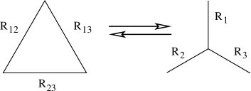
Figure 2: Illustration of the $\Delta$-Y and Y-$\Delta$ transforms.

The basic idea of the $\Delta$-Y transform is illustrated in Fig. 2. Any triangular arrangement of resistors $R_{12}$, $R_{13}$, and $R_{23}$ within a larger circuit can be replaced by a star, with resistances $R_{1}$, $R_{2}$, and $R_{3}$, such that all resistances between any two points among the three vertices in the triangle and the star are the same. The conditions that all two-point resistances are the same are:

$$(R_{1}+R_{2})=\left[R_{12}^{-1}+(R_{13}+R_{23})^{-1}\right]^{-1}\equiv a_{12}\qquad\textrm{+ cyclic permutations}.$$

Solving for $R_{1},R_{2}$, and $R_{3}$ gives $R_{1}=\frac{1}{2}(a_{12}-a_{23}+a_{13})$ + cyclic permutations; the explicit result in terms of the $R_{ij}$ is:

$$R_{1}=\frac{R_{12}R_{13}}{R_{12}+R_{13}+R_{23}}\qquad\textrm{+ cyclic permutations},$$ (12)

as well as the companion result for the conductances $G_{i}=R_{i}^{-1}$:

$$G_{1}=\frac{G_{12}G_{13}+G_{12}G_{23}+G_{13}G_{23}}{G_{23}}\qquad\textrm{+ cyclic permutations}.$$

These relations allow one to replace any triangle by a star to reduce an electrical network.

However, sometimes we need to replace a star by a triangle to simplify a network. To construct the inverse Y-$\Delta$ transform, notice that the $\Delta$-Y transform gives the resistance ratios $R_{1}/R_{2}=R_{13}/R_{23}$ + cyclic permutations, from which $R_{13}=R_{12}(R_{3}/R_{2})$ and $R_{23}=R_{12}(R_{3}/R_{1})$. Substituting these last two results in Eq. (12), we eliminate $R_{13}$ and $R_{23}$ and thus solve for $R_{12}$ in terms of the $R_{i}$:

$$R_{12}=\frac{R_{1}R_{2}+R_{1}R_{3}+R_{2}R_{3}}{R_{3}}\qquad\textrm{+ cyclic permutations},$$ (13)

and similarly for $G_{ij}=R_{ij}^{-1}$. To appreciate the utility of the $\Delta$-Y and Y-$\Delta$ transforms, the reader is invited to apply them on the Wheatstone bridge.

When employed judiciously and repeatedly, these transforms systematically reduce planar lattice circuits to a single bond, and thus provide a powerful approach to calculate the conductance of large networks near the percolation threshold. We will return to this aspect of the problem in Sec. IV.2.

III.5 Effective Medium Theory

Effective medium theory (EMT) determines the macroscopic conductance of a random resistor network by a homogenization procedure [2, 3, 16, 17, 18, 19] that is reminiscent of the Curie-Weiss effective field theory of magnetism. The basic idea in EMT is to replace the random network by an effective homogeneous medium in which the conductance of each resistor is determined self-consistently to optimally match the conductances of the original and homogenized systems. EMT is quite versatile and has been applied, for example, to estimate the dielectric constant of dielectric composites and the conductance of conducting composites. Here we focus on the conductance of random resistor networks, in which each resistor (with conductance $g_{0}$) is present with probability $p$ and absent with probability $1-p$. The goal is to determine the conductance as a function of $p$.

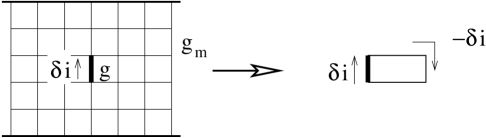
Figure 3: Illustration of EMT. (left) The homogenized network with conductances $g_{m}$ and one bond with conductance $g$. (right) The equivalent circuit to the lattice.

To implement EMT, we first replace the random network by an effective homogeneous medium in which each bond has the same conductance $g_{m}$ (Fig. 3). If a voltage is applied across this effective medium, there will be a potential drop $V_{m}$ and a current $I_{m}=g_{m}V_{m}$ across each bond. The next step in EMT is to assign one bond in the effective medium a conductance $g$ and adjust the external voltage to maintain a fixed total current $I$ passing through the network. Now an additional current $\delta i$ passes through the conductor $g$. Consequently, a current $-\delta i$ must flow through one terminal of $g$ to the other terminal via the remainder of the network (Fig. 3). This current perturbation leads to an additional voltage drop $\delta V$ across $g$. Thus the current-voltage relations for the marked bond and the remainder of the network are

$$I_{m}+\delta i = g(V_{m}+\delta V)$$

$$-\delta i = G_{ab}\,\delta V,$$ (14)

where $G_{ab}$ is the conductance of the rest of the lattice between the terminals of the conductor $g$.

The last step in EMT is to require that the mean value $\delta V$ averaged over the probability distribution of individual bond conductances is zero. Thus the effective medium “matches” the current-carrying properties of the original network. Solving Eq. (III.5) for $\delta V$, and using the probability distribution $P(g)=p\delta(g-g_{0})+(1-p)\delta(g)$ appropriate for the random resistor network, we obtain

$$\langle\delta V\rangle=V_{m}\left[\frac{(g_{m}-g_{0})p}{(G_{ab}+g_{0})}+\frac{g_{m}(1-p)}{G_{ab}}\right]=0.$$ (15)

It is now convenient to write $G_{ab}=\alpha g_{m}$, where $\alpha$ is a lattice-dependent constant of the order of one. With this definition, Eq. (15) simplifies to

$$g_{m}=g_{o}\frac{p(1+\alpha)-1}{\alpha}.$$ (16)

The value of $\alpha$—the proportionality constant for the conductance of the initial lattice with a single bond removed—can usually be determined by a symmetry argument of the type presented in Sec. II. For example, for the triangular lattice (coordination number 6), the conductance $G_{ab}=2g_{m}$ and $\alpha=2$. For the hypercubic lattice in $d$ dimensions (coordination number $z=2^{d}$), $G_{ab}=\frac{z-2}{2}\,g_{m}$.

The main features of the effective conductance $g_{m}$ that arises from EMT are: (i) the conductance vanishes at a lattice-dependent percolation threshold $p_{c}=1/(1+\alpha)$; for the hypercubic lattice $\alpha=\frac{z-2}{2}$ and the percolation threshold $p_{c}=\frac{2}{z}=2^{1-d}$ (fortuitously reproducing the exact percolation threshold in two dimensions); (ii) the conductance varies linearly with $p$ and vanishes linearly in $p-p_{c}$ as $p$ approaches $p_{c}$ from above. The linearity of the effective conductance away from the percolation threshold accords with numerical and experimental results. However, EMT fails near the percolation threshold, where large fluctuations arise that invalidate the underlying assumptions of EMT. In this regime, alternative methods are needed to estimate the conductance.

IV Conduction Near the Percolation Threshold

IV.1 Scaling Behavior

EMT provides a qualitative but crude picture of the current-carrying properties of a random resistor network. While EMT accounts for the existence of a percolation transition, it also predicts a linear dependence of the conductance on $p$. However, near the percolation threshold it is well known that the conductance varies non-linearly in $p-p_{c}$ near $p_{c}$ [29]. This non-linearity defines the conductance exponent $t$ by

$$G\sim(p-p_{c})^{t}\qquad p\downarrow p_{c},$$ (17)

and much research on random resistor networks [29] has been done to determine this exponent. The conductance exponent generically depends only on the spatial dimension of the network and not on any other details (a notable exception, however, is when link resistances are broadly distributed, see [30, 31]). This universality is one of the central tenets of the theory of critical phenomena [32, 33]. For percolation, the mechanism underlying universality is the absence of a characteristic length scale; as illustrated in Fig. 4, clusters on all length scales exist when a network is close to the percolation threshold.

The scale of the largest cluster defines the correlation length $\xi$ by $\xi\sim(p_{c}-p)^{-\nu}$ as $p\to p_{c}$. The divergence in $\xi$ also applies for $p>p_{c}$ by defining the correlation length as the typical size of finite clusters only (Fig. 4), thus eliminating the infinite percolating cluster from consideration. At the percolation threshold, clusters on all length scales exist, and the absence of a characteristic length implies that the singularity in the conductance should not depend on microscopic variables. The only parameter remaining upon which the conductance exponent $t$ can depend upon is the spatial dimension $d$ [32, 33]. As typifies critical phenomena, the conductance exponent has a constant value in all spatial dimensions $d>d_{c}$, where $d_{c}$ is the upper critical dimension which equals 6 for percolation [34]. Above this critical dimension, mean-field theory (not to be confused with EMT) gives the correct values of critical exponents.

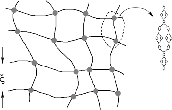
Figure 4: (left) Realization of bond percolation on a $25\times 25$ square lattice at p=0.505. (Right) Schematic picture of the nodes (shaded circles), links and blobs picture of percolation for $p\,\,{\mathrel{\raise 1.29167pt\hbox{$>$\kern-7.5pt\lower 4.30554pt\hbox{$\sim$}}}}\,\,p_{c}$.

While there does not yet exist a complete theory for the dimension dependence of the conductance exponent below the critical dimension, a crude but useful nodes, links, and blobs picture of the infinite cluster [35, 36, 37] provides partial information. The basic idea of this picture is that for $p\,{\mathrel{\raise 1.29167pt\hbox{$>$\kern-7.5pt\lower 4.30554pt\hbox{$\sim$}}}}\,p_{c}$, a large system has an irregular network-like topology that consists of quasi-linear chains that are separated by the correlation length $\xi$ (Fig. 4). For a macroscopic sample of linear dimension $L$ with a bus bar-geometry, the percolating cluster above $p_{c}$ then consists of $(L/\xi)^{d-1}$ statistically identical chains in parallel, in which each chain consists of $L/\xi$ macrolinks in series, and the macrolinks consists of nested blob-like structures

The conductance of a macrolink is expected to vanish as $(p-p_{c})^{\zeta}$, with $\zeta$ a new unknown exponent. Although a theory for the conductance of a single macrolink, and even a precise definition of a macrolink, is still lacking, the nodes, links, and blobs picture provides a starting point for understanding the dimension dependence of the conductance exponent. Using the rules for combining parallel and series conductances, the conductance of a large resistor network of linear dimension $L$ is then

$$G(p,L)\sim\left(\frac{L}{\xi}\right)^{d-1}\frac{(p-p_{c})^{\zeta}}{L/\xi}\sim L^{d-2}\,(p-p_{c})^{(d-2)\nu+\zeta}.$$ (18)

In the limit of large spatial dimension, we expect that a macrolink is merely a random walk between nodes. Since the spatial separation between nodes is $\xi$, the number of bonds in the macrolink, and hence its resistance, scales as $\xi^{2}$ [38]. Using the mean-field result $\xi\sim(p-p_{c})^{-1/2}$, the resistance of the macrolink scales as $(p-p_{c})^{-1}$ and thus the exponent $\zeta=1$. Using the mean-field exponents $\nu=1/2$ and $\zeta=1$ at the upper critical dimension of $d_{c}=6$, we then infer the mean-field value of the conductance exponent $t=3$ [34, 38, 39].

Scaling also determines the conductance of a finite-size system of linear dimension $L$ exactly at the percolation threshold. Although the correlation length formally diverges when $p-p_{c}=0$, $\xi$ is limited by $L$ in a finite system of linear dimension $L$. Thus the only variable upon which the conductance can depend is $L$ itself. Equivalently, deviations in $p-p_{c}$ that are smaller than $L^{-1/\nu}$ cannot influence critical behavior because $\xi$ can never exceed $L$. Thus to determine the dependence of a singular observable for a finite-size system at $p_{c}$, we may replace $(p-p_{c})$ by $L^{-1/\nu}$. By this prescription, the conductance at $p_{c}$ of a large finite-size system of linear dimension $L$ becomes

$$G(p_{c},L)\sim L^{d-2}(L^{-1/\nu})^{(d-2)\nu+\zeta}\sim L^{-\zeta/\nu}~{}.$$ (19)

In this finite-size scaling [29], we fix the occupation probability to be exactly at $p_{c}$ and study the dependence of an observable on $L$ to determine percolation exponents. This approach provides a convenient and more accurate method to determine the conductance exponent compared to studying the dependence of the conductance of a large system as a function of $p-p_{c}$.

IV.2 Conductance Exponent

In percolation and in the random resistor network, much effort has been devoted to computing the exponents that characterize basic physical observables—such as the correlation length $\xi$ and the conductance $G$—to high precision. There are several reasons for this focus on exponents. First, because of the universality hypothesis, exponents are a meaningful quantifier of phase transitions. Second, various observables near a phase transition can sometimes be related by a scaling argument that leads to a corresponding exponent relation. Such relations may provide a decisive test of a theory that can be checked numerically. Finally, there is the intellectual challenge of developing accurate numerical methods to determine critical exponents. The best such methods have become quite sophisticated in their execution.

A seminal contribution was the “theorists’ experiment” of Last and Thouless [40] in which they punched holes at random in a conducting sheet of paper and measured the conductance of the sheet as a function of the area fraction of conducting material. They found that the conductance vanished faster than linearly with $(p-p_{c})$; here $p$ corresponds to the area fraction of the conductor. Until this experiment, there was a sentiment that the conductance should be related to the fraction of material in the percolating cluster [41]—the percolation probability $P(p)$—a quantity that vanished slower than linearly with $(p-p_{c})$. The reason for this disparity is that in a resistor network, much of the percolating cluster consists of dangling ends—bonds that carry no current—and thus make no contribution to the conductance. A natural geometrical quantity that ought to be related to the conductance is the fraction of bonds $B(p)$ in the conducting backbone—the subset of the percolating cluster without dangling ends. However, a clear relation between the conductivity and a geometrical property of the backbone has not yet been established.

Analytically, there are primary two methods that have been developed to compute the conductance exponent: the renormalization group [42, 43, 44, 45] and low-density series expansions [46, 47, 48]. In the real-space version of the renormalization group, the evolution of conductance distribution under length rescaling is determined, while the momentum-space version involves a diagrammatic implementation of this length rescaling in momentum space. The latter is a perturbative approach away from mean-field theory in the variable $6-d$ that become exact as $d\to 6$.

Considerable effort has been devoted to determining the conductance exponent by numerical and algorithmic methods. Typically, the conductance is computed for networks of various linear dimensions $L$ at $p=p_{c}$, and the conductance exponent is extracted from the $L$ dependence of the conductance, which should vanish as $L^{-\zeta/\nu}$. An exact approach, but computationally impractical for large networks, is Gauss elimination to invert the conductance matrix [49]. A simple approximate method is Gauss relaxation [50, 51, 52, 53, 54] (and its more efficient variant of Gauss-Seidel relaxation [55]). This method uses Eq. (2) as the basis for an iteration scheme, in which the voltage $V_{i}$ at node $i$ at the $n^{\rm th}$ update step is computed from (2) using the values of $V_{j}$ at the $(n-1)^{\rm st}$ update in the right-hand side of this equation. However, one can do much better by the conjugate gradient algorithm [56] and speeding up this method still further by Fourier acceleration methods [57].

Another computational approach is based on the node elimination method, in which the $\Delta$-Y and Y-$\Delta$ transforms are used to successively eliminate bonds from the network and ultimately reduce a large network to a single bond [8, 9, 10]. In a different vein, the transfer matrix method has proved to be extremely accurate and efficient [58, 59, 60, 61]. The method is based on building up the network one bond at a time and immediately calculating the conductance of the network after each bond addition. This method is most useful when applied to very long strips of transverse dimension $L$ so that a single realization gives an accurate value for the conductance.

As a result of these investigations, as well as by series expansions for the conductance, the following exponents have been found. For $d=2$, where most of the computational effort has been applied, the best estimate [61] for the exponent $t$ (using $\zeta=t$ in $d=2$ only) is $t=1.299\pm 0.002$. One reason for the focus on two dimensions is that early estimates for $t$ were tantalizingly close to the correlation length exponent $\nu$ that is now known to exactly equal 4/3 [62]. Another such connection was the Alexander-Orbach conjecture [63], which predicted $t=91/72=1.2638\ldots$, but again is incompatible with the best numerical estimate for $t$. In $d=3$, the best available numerical estimate for $t$ appears to be $t=2.003\pm 0.047$ [64, 65], while the low concentration series method gives an equally precise result of $t=2.02\pm 0.05$ [47, 48]. These estimates are just compatible with the rigorous bound that $t\leq 2$ in $d=3$ [66, 67]. In greater than three dimensions, these series expansions give $t=2.40\pm 0.03$ for $d=4$ and $t=2.74\pm 0.03$ for $d=5$, and the dimension dependence is consistent with $t=3$ when $d$ reaches 6.

V Voltage Distribution in Random Networks

V.1 Multifractal Scaling

While much research has been devoted to understanding the critical behavior of the conductance, it was realized that the distribution of voltages across each resistor of the network was quite rich and exhibited multifractal scaling [68, 69, 70, 71]. Multifractality is a generalization of fractal scaling in which the distribution of an observable is sufficiently broad that different moments of the distribution scale independently. Such multifractal scaling arises in phenomena as diverse as turbulence [72, 73], localization [74], and diffusion-limited aggregation [75, 76]. All these diverse examples showed scaling properties that were much richer than first anticipated.

To make the discussion of multifractality concrete, consider the example of the Maxwell-Boltzmann velocity distribution of a one-dimensional ideal gas

$$P(v)=\sqrt{\frac{m}{2\pi k_{B}T}}\,e^{-mv^{2}/2k_{B}T}\equiv\frac{1}{\sqrt{2\pi v_{\rm th}^{2}}}\,e^{-v^{2}/2v_{\rm th}^{2}},$$

where $k_{B}$ is Boltzmann’s constant, $m$ is the particle mass, $T$ is the temperature, and $v_{\rm th}=\sqrt{k_{B}T/m}$ is the characteristic thermal velocity. The even integer moments of the velocity distribution are

$$\langle(v^{2})^{n}\rangle\propto(v_{\rm th}^{\,\,2})^{n}\equiv(v_{\rm th}^{\,\,2})^{p(n)}.$$

Thus a single velocity scale, $v_{\rm th}$, characterizes all positive moments of the velocity distribution. Alternatively, the exponent $p(n)$ is linear in $n$. This linear dependence of successive moment exponents characterizes single-parameter scaling. The new feature of multifractal scaling is that a wide range of scales characterizes the voltage distribution (Fig. 5). As a consequence, the moment exponent $p(n)$ is a non-linear function of $n$.

One motivation for studying the voltage distribution is its relation to basic aspects of electrical conduction. If a voltage $V=1$ is applied across a resistor network, then the conductance $G$ and the total current flow $I$ are equal: $I=G$. Consider now the power dissipated through the network $P=IV=GV^{2}\to G$. We may also compute the dissipated power by adding up these losses in each resistor to give

$$P=G=\sum_{ij}g_{ij}V_{ij}^{2}\to\sum_{ij}V_{ij}^{2}=\sum_{V}V^{2}\,N(V).$$ (20)

Here $g_{ij}=1$ is the conductance of resistor $ij$, and $V_{ij}$ is the corresponding voltage drop across this bond. In the last equality, $N(V)$ is the number of resistors with a voltage drop $V$. Thus the conductance is just the second moment of the distribution of voltage drops across each bond in the network.

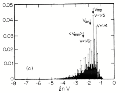
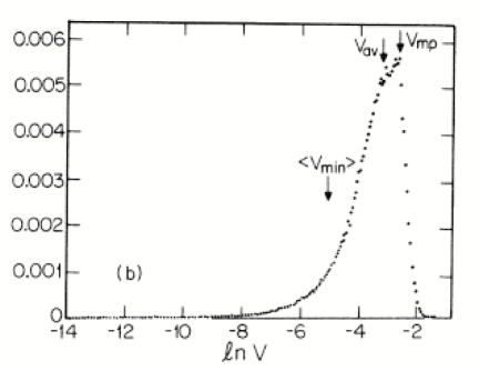
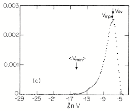
Figure 5: The voltage distribution on an $L\times L$ square lattice random resistor network at the percolation threshold for (a) $L=4$ (exact), (b) $L=10$, and (c) $L=130$. The latter two plots are based on simulation data. For $L=4$, a number of peaks, that correspond to simple rational fractions of the unit potential drop, are indicated. Also shown are the average voltage over all realizations, $V_{\rm av}$, the most probable voltage, $V_{\rm mp}$, and the average of the minimum voltage in each realization, $\langle V_{\rm min}\rangle$. [Reprinted from Ref. [69]].

From the statistical physics perspective it is natural to study other moments of the voltage distribution and the voltage distribution itself. Analogous to the velocity distribution, we define the family of exponents $p(k)$ for the scaling dependence of the voltage distribution at $p=p_{c}$ by

$$\mathcal{M}(k)\equiv\sum_{V}N(V)V^{k}\sim L^{-p(k)/\nu}.$$ (21)

Since $\mathcal{M}(2)$ is just the network conductance, $p(2)=\zeta$. Other moments of the voltage distribution also have simple interpretations. For example, $\langle V^{4}\rangle$ is related to the magnitude of the noise in the network [71, 77], while $\langle V^{k}\rangle$ for $k\to\infty$ weights the bonds with the highest currents, or the “hottest” bonds of the network, most strongly, and they help understand the dynamics of fuse networks of failure [78]. On the other hand, negative moments weight low-current bonds more strongly and emphasize the low-voltage tail of the distribution. For example, $\mathcal{M}(-1)$ characterizes hydrodynamic dispersion [79], in which passive tracer particles disperse in a network due to a multiplicity of network paths. In hydrodynamics dispersion, the transit time across each bond is proportional to the inverse of the current in the bond, while the probability for tracer to enter a bond is proportional to the entering current. As a result, the $k^{\rm th}$ moment of the transit time distribution varies as $\mathcal{M}(-k+1)$, so that the quantity that quantifies dispersion, $\langle t^{2}\rangle-\langle t\rangle^{2}$, scales as $\mathcal{M}(-1)$.

A simple fractal model [80, 81, 82] of the conducting backbone (Fig. 6) illustrates the multifractal scaling of the voltage distribution near the percolation threshold [68]. To obtain the $N^{\rm th}$-order structure, each bond in the $(N-1)^{\rm st}$ iteration is replaced by the first-order structure. The resulting fractal has a hierarchical embedding of links and blobs that captures the basic geometry of the percolating backbone. Between successive generations, the length scale changes by a factor of 3, while the number of bonds changes by a factor of 4. Defining the fractal dimension $d_{f}$ as the scaling relation between mass ($M=4^{N}$) and the length scale ($\ell=3^{N}$) via $M\sim\ell^{d_{f}}$, gives a fractal dimension $d_{f}=\ln 4/\ln 3$.

Figure 6: The first few iterations of a hierarchical model.

Now let’s determine the distribution of voltage drops across the bonds. If a unit voltage is applied at the opposite ends of a first-order structure ($N=1$) and each bond is a 1 ohm resistor, then the two resistors in the central bubble each have a voltage drop of 1/5, while the two resistors at the ends have a voltage drop 2/5. In an $N^{\rm th}$-order hierarchy, the voltage of any resistor is the product of these two factors, with number of times each factor occurs dependent on the level of embedding of a resistor within the blobs. It is a simple exercise to show that the voltage distribution is [68]

$$N(V(j))=2^{N}\binom{N}{j}~{},$$ (22)

where the voltage $V(j)$ can take the values $2^{j}/5^{N}$ (with $j=0,1,\ldots,N$). Because $j$ varies logarithmically in $V$, the voltage distribution is log binomial [83]. Using this distribution in Eq. (21), the moments of the voltage distribution are

$$\mathcal{M}(k)=\left[\frac{2(1+2^{k})}{5^{k}}\right]^{N}.$$ (23)

In particular, the average voltage, $\mathcal{M}(1)/\mathcal{M}(0)\equiv V_{\rm av}$ equals $\bigl{(}\frac{3/2}{5}\bigr{)}^{N}$, which is very different from the most probable voltage, $V_{\rm mp}=\bigl{(}\frac{\sqrt{2}}{5}\bigr{)}^{N}$ as $N\rightarrow\infty$. The underlying multiplicativity of the bond voltages is the ultimate source of the large disparity between the average and most probable values.

To calculate the moment exponent $p(k)$, we first need to relate the iteration index $N$ to a physical length scale. For percolation, the appropriate relation is based on Coniglio’s theorem [84], which is a simple but profound statement about the structure of the percolating cluster. This theorem states that the number of singly-connected bonds in a system of linear dimension $L$, $\mathcal{N}_{s}$, varies as $L^{1/\nu}$. Singly-connected bonds are those that would disconnect the network if they were cut. An equivalent form of the theorem is $\mathcal{N}_{s}=\frac{\partial p^{\prime}}{\partial p}$, where $p^{\prime}$ is the probability that a spanning cluster exists in the system. This relation reflects the fact that when $p$ is decreased slightly, $p^{\prime}$ changes only if a singly-connected bond happens to be deleted.

In the $N^{\rm th}$-order hierarchy, the number of such singly-connected links is simply $2^{N}$. Equating these two gives an effective linear dimension, $L=2^{N\nu}$. Using this relation in (23), the moment exponent $p(k)$ is

$$p(k)=k-1+\left[k\ln\left(5/4\right)-\ln(1+2^{-k})\right]/\ln 2.$$ (24)

Because each $p(k)$ is independent, the moments of the voltage distribution are characterized by an infinite set of exponents. Eq. (24) is in excellent agreement with numerical data for the voltage distribution in two-dimensional random resistor networks at the percolation threshold [69]. A similar multifractal behavior was also found for the voltage distribution of the resistor network at the percolation threshold in three dimensions [85].

Maximum Voltage

An important aspect of the voltage distribution, both because of its peculiar scaling properties [56] and its application to breakdown problems [78, 56], is the maximum voltage in a network. The salient features of this maximum voltage are: (i) logarithmic scaling as a function of system size [56, 86, 87, 89, 88], and (ii) non-monotonic dependence on the resistor concentration $p$ [90]. The former property is a consequence of the expected size of the largest defect in the network that gives maximal local currents. Here, we use the terms maximum local voltage and maximum local current interchangeably because they are equivalent.

To find the maximal current, we first need to identify the optimal defects that lead to large local currents. A natural candidate is an ellipse [56, 86] with major and minor axes $a$ and $b$ (continuum), or its discrete analog of a linear crack (hyperplanar crack in greater than two dimensions) in which $n$ resistors are missing (Fig. 7). Because current has to detour around the defect, the local current at the ends of the defect is magnified. For the continuum problem, the current at the tip of the ellipse is $I_{\rm tip}=I_{0}(1+a/b)$, where $I_{0}$ is the current in the unperturbed system [56]. For the maximum current in the lattice system, one must integrate the continuum current over a one lattice spacing and identify $a/b$ with $n$ [89]. This approach gives the maximal current at the tip of a crack $I_{\rm max}\propto(1+n^{1/2})$ in two dimensions and as $I_{\rm max}\propto(1+n^{1/2(d-1)})$ in $d$ dimensions.

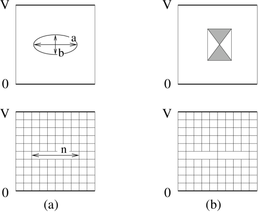
Figure 7: Defect configurations in two dimensions. (a) An ellipse and its square lattice counterpart, (b) a funnel, with the region of good conductor shown shaded, and a 2-slit configuration on the square lattice.

Next, we need to find the size of the largest defect, which is an extreme-value statistics exercise [91]. For a linear crack, each broken bond occurs with probability $1-p$, so that the probability for a crack of length $n$ is $(1-p)^{n}\equiv e^{-an}$, with $a=-\ln(1-p)$. In a network of volume $L^{d}$, we estimate the size of the largest defect by $L^{d}\int_{n_{\rm max}}^{\infty}e^{-an}\,dx=1$; that is, there exists of the order of one defect of size $n_{\rm max}$ or larger in the network [91]. This estimate gives $n_{\rm max}$ varying as $\ln L$. Combining this result with the current at the tip of a crack of length $n$, the largest current in a system of linear dimension $L$ scales as $(\ln L)^{1/2(d-1)}$.

A more thorough analysis shows, however, that a single crack is not quite optimal. For a continuum two-component network with conductors of resistance 1 with probability $p$ and with resistance $r>1$ with probability $1-p$, the configuration that maximizes the local current is a funnel [87, 88]. For a funnel of linear dimension $\ell$, the maximum current at the apex of the funnel is proportional to $\ell^{1-\nu}$, where $\nu=\frac{4}{\pi}\tan^{-1}(r^{-1/2})$ [87, 88]. The probability to find a funnel of linear dimension $\ell$ now scales as $e^{-b\ell^{2}}$ (exponentially in its area), with $b$ a constant. By the same extreme statistics reasoning given above, the size of the largest funnel in a system of linear dimension $L$ then scales as $(\ln L)^{1/2}$, and the largest expected current correspondingly scales as $(\ln L)^{(1-\nu)/2}$. In the limit $r\to\infty$, where one component is an insulator, the optimal discrete configuration in two dimensions becomes two parallel slits, each of length $n$, between which a single resistor remains [89]. For this two-slit configuration, the maximum current is proportional to $n$ in two dimensions, rather than $n^{1/2}$ for the single crack. Thus the maximal current in a system of linear dimension $L$ scales as $\ln L$ rather than as a fractional power of $\ln L$.

The $p$ dependence of the maximum voltage is intriguing because it is non-monotonic. As $p$, the fraction of occupied bonds, decreases from 1, less total current flows (for a fixed overall voltage drop) because the conductance is decreasing, while local current in a funnel is enhanced because such defects grow larger. The competition between these two effects leads to $V_{\rm max}$ attaining its peak at $p_{\rm peak}$ above the percolation threshold that only slowly approaches $p_{c}$ as $L\to\infty$. An experimental manifestation of this non-monotonicity in $V_{\rm max}$ occurred in a resistor-diode network [92], where the network reproducibly burned (solder connections melting and smoking) when $p\simeq 0.77$, compared to a percolation threshold of $p_{c}\simeq 0.58$. Although the directionality constraint imposed by diodes enhances funneling, similar behavior should occur in a random resistor network.

Figure 8: The bubble model: a chain of $L$ bubbles in series, each consisting of $w$ bonds in parallel. Each bond is independently present with probability $p$.

The non-monotonic $p$ dependence of $V_{\rm max}$ can be understood within the quasi-one-dimensional “bubble” model [90] that captures the interplay between local funneling and overall current reduction as $p$ decreases (Fig. 8). Although this system looks one-dimensional, it can be engineered to reproduce the percolation properties of a system in greater than one dimension by choosing the length $L$ to scale exponentially with the width $w$. The probability for a spanning path in this structure is

$$p^{\prime}=\left[1-(1-p)^{w}\right]^{L}\to\exp[-L\,e^{-pw}]\qquad L,w\to\infty,$$ (25)

which suddenly changes from 0 to 1—indicative of percolation—at a threshold that lies strictly within (0,1) as $L\to\infty$ and $L\sim e^{w}$. In what follows, we take $L=2^{w}$, which gives $p_{c}=1/2$.

To determine the effect of bottlenecking, we appeal to the statement of Coniglio’s theorem [84], $\frac{\partial p^{\prime}}{\partial p}$ equals the average number of singly-connected bonds in the system. Evaluating $\frac{\partial p^{\prime}}{\partial p}$ in Eq. (25) at the percolation threshold of $p_{c}=\frac{1}{2}$ gives

$$\frac{\partial p^{\prime}}{\partial p}=w+{\cal O}(e^{-w})\sim\ln L.$$ (26)

Thus at $p_{c}$ there are $w\sim\ln L$ bottlenecks. However, current focusing due to bottlenecks is substantially diluted because the conductance, and hence the total current through the network, is small at $p_{c}$. What is needed is a single bottleneck of width 1. One such bottleneck ensures the total current flow is still substantial, while the narrowing to width 1 endures that the focusing effect of the bottleneck is maximally effective.

Clearly, a single bottleneck of width 1 occurs above the percolation threshold. Thus let’s determine when a such an isolated bottleneck of width 1 first appears as a function of $p$. The probability that a single non-empty bubble contains at least two bonds is $(1-q^{w}-wpq^{w-1})/(1-q^{w})$, where $q=1-p$. Then the probability $P_{1}(p)$ that the width of the narrowest bottleneck has width 1 in a chain of $L$ bubbles is

$$P_{1}(p)=1-\left(1-\frac{wpq^{w-1}}{1-q^{w}}\right)^{L}\sim 1-\exp\left(-Lw\frac{p}{q(1-q^{w})}\,e^{-pw}\right).$$ (27)

The subtracted term is the probability that $L$ non-empty bubbles contain at least two bonds, and then $P_{1}(p)$ is the complement of this quantity. As $p$ decreases from 1, $P_{1}(p)$ sharply increases from 0 to 1 when the argument of the outer exponential becomes of the order of 1; this change occurs at $\hat{p}\sim p_{c}+{\cal O}(\ln(\ln L)/\ln L)$. At this point, a bottleneck of width 1 first appears and therefore $V_{\rm max}$ also occurs for this value of $p$.

VI Random Walks and Resistor Networks

VI.1 The Basic Relation

We now discuss how the voltages at each node in a resistor network and the resistance of the network are directly related to first-passage properties of random walks [94, 20, 95, 93]. To develop this connection, consider a random walk on a finite network that can hop between nearest-neighbor sites $i$ to $j$ with probability $p_{ij}$ in a single step. We divide the boundary points of the network into two disjoint classes, $\mathcal{B}_{+}$ and $\mathcal{B}_{-}$, that we are free to choose; a typical situation is the geometry shown in Fig. 9. We now ask: starting at an arbitrary point $i$, what is the probability that the walk eventually reaches the boundary set $\mathcal{B}_{+}$ without first reaching any node in $\mathcal{B}_{-}$? This quantity is termed the exit probability $\mathcal{E}_{+}(i)$ (with an analogous definition for the exit probability $\mathcal{E}_{-}(i)=1-\mathcal{E}_{+}(i)$ to $\mathcal{B}_{-}$).

We obtain the exit probability ${\mathcal{E}}_{+}(i)$ by summing the probabilities for all walk trajectories that start at $i$ and reach a site in $\mathcal{B}_{+}$ without touching any site in $\mathcal{B}_{-}$ (and similarly for ${\mathcal{E}}_{-}(i)$). Thus

$${\mathcal{E}}_{\pm}(i)=\sum_{p_{\pm}}{\mathcal{P}}_{p_{\pm}}(i),$$ (28)

where ${\mathcal{P}}_{p_{\pm}}(i)$ denotes the probability of a path from $i$ to $\mathcal{B}_{\pm}$ that avoids $\mathcal{B}_{\mp}$. The sum over all these restricted paths can be decomposed into the outcome after one step, when the walk reaches some intermediate site $j$, and the sum over all path remainders from $j$ to $\mathcal{B}_{\pm}$. This decomposition gives

$${\mathcal{E}}_{\pm}(i) = \sum_{j}p_{ij}\,{\mathcal{E}}_{\pm}(j).$$ (29)

Thus ${\mathcal{E}}_{\pm}(i)$ is a harmonic function because it equals a weighted average of ${\mathcal{E}}_{\pm}$ at neighboring points, with weighting function $p_{ij}$. This is exactly the same relation obeyed by the node voltages in Eq. (2) for the corresponding resistor network when we identify the single-step hopping probabilities $p_{ij}$ with the conductances $g_{ij}/\sum_{j}g_{ij}$. We thus have the following equivalence:

• Let the boundary sets $\mathcal{B}_{+}$ and $\mathcal{B}_{-}$ in a resistor network be fixed at voltages 1 and 0 respectively, with $g_{ij}$ the conductance of the bond between sites $i$ and $j$. Then the voltage at any interior site $i$ coincides with the probability for a random walk, which starts at $i$, to reach $\mathcal{B}_{+}$ before reaching $\mathcal{B}_{-}$, when the hopping probability from $i$ to $j$ is $p_{ij}=g_{ij}/\sum_{j}g_{ij}$.

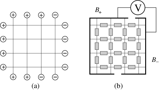
Figure 9: (a) Lattice network with boundary sites $\mathcal{B}_{+}$ or $\mathcal{B}_{-}$. (b) Corresponding resistor network in which each rectangle is a 1 ohm resistor. The sites in $\mathcal{B}_{+}$ are all fixed at potential $V=1$, and sites in $\mathcal{B}_{-}$ are all grounded.

If all the bond conductances are the same—corresponding to single-step hopping probabilities in the equivalent random walk being identical—then Eq. (29) is just the discrete Laplace equation. We can then exploit this correspondence between conductances and hopping probabilities to infer non-trivial results about random walks and about resistor networks from basic electrostatics. This correspondence can also be extended in a natural way to general random walks with a spatially-varying bias and diffusion coefficient, and to continuous media.

The consequences of this equivalence between random walks and resistor networks is profound. As an example [93], consider a diffusing particle that is initially at distance $r_{0}$ from the center of a sphere of radius $a<r_{0}$ in otherwise empty $d$-dimensional space. By the correspondence with electrostatics, the probability that this particle eventually hits the sphere is simply the electrostatic potential at $r_{0}$, ${\mathcal{E}}_{-}(r_{0})=(a/r_{0})^{d-2}$ !

VI.2 Network Resistance and Pólya’s Theorem

An important extension of the relation between exit probability and node voltages is to infinite resistor networks. This extension provides a simple connection between the classic recurrence/transience transition of random walks on a given network [94, 20, 95, 93] and the electrical resistance of this same network [15]. Consider a symmetric random walk on a regular lattice in $d$ spatial dimensions. Suppose that the walk starts at the origin at $t=0$. What is the probability that the walk eventually returns to its starting point? The answer is strikingly simple:

• For $d\leq 2$, a random walk is certain to eventually return to the origin. This property is known as recurrence.

• For $d>2$, there is a non-zero probability that the random walk will never return to the origin. This property is known as transience.

Let’s now derive the transience and recurrence properties of random walks in terms of the equivalent resistor network problem. Suppose that the voltage $V$ at the boundary sites $\mathcal{B}_{+}$ is set to one. Then by Kirchhoff’s law, the total current entering the network is

$$I=\sum_{j}(1-V_{j})g_{+j}=\sum_{j}(1-V_{j})p_{+j}\sum_{k}g_{+k}.$$ (30)

Here $g_{+j}$ is the conductance of the resistor between $\mathcal{B}_{+}$ and a neighboring site $j$, and $p_{+j}=g_{+j}/\sum_{j}g_{+j}$. Because the voltage $V_{j}$ also equals the probability for the corresponding random walk to reach $\mathcal{B}_{+}$ without reaching $\mathcal{B}_{-}$, the term $V_{j}\,p_{+j}$ is just the probability that a random walk starts at $\mathcal{B}_{+}$, makes a single step to one of the sites $j$ adjacent to $\mathcal{B}_{+}$ (with hopping probability $p_{ij}$), and then returns to $\mathcal{B}_{+}$ without reaching $\mathcal{B}_{-}$. We therefore deduce that

$$I=\sum_{j}(1-V_{j})g_{+j} = \sum_{k}g_{+k}\sum_{j}(1-V_{j})p_{+j}$$ (31)

$$= \sum_{k}g_{+k}\times(1-{\rm return\ probability})$$

$$= \sum_{k}g_{+k}\times{\rm escape\ probability}.$$

Here “escape” means that the random walk reaches the set $\mathcal{B}_{-}$ without returning to a node in $\mathcal{B}_{+}$.

On the other hand, the current and the voltage drop across the network are related to the conductance $G$ between the two boundary sets by $I=GV=G$. From this fact, Eq. (31) gives the fundamental result

$${\rm escape\ probability}\equiv P_{\rm escape}=\frac{G}{\sum_{k}g_{+k}}.$$ (32)

Suppose now that a current $I$ is injected at a single point of an infinite network, with outflow at infinity (Fig. 10). Thus the probability for a random walk to never return to its starting point, is simply proportional to the conductance $G$ from this starting point to infinity of the same network. Thus a subtle feature of random walks, namely, the escape probability, is directly related to currents and voltages in an equivalent resistor network.

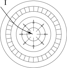
Figure 10: Decomposition of a conducting medium into concentric shells, each of which consists of fixed-conductance blocks. A current $I$ is injected at the origin and flows radially outward through the medium.

Part of the reason why this connection is so useful is that the conductance of the infinite network for various spatial dimensions can be easily determined, while a direct calculation of the return probability for a random walk is more difficult. In one dimension, the conductance of an infinitely long chain of identical resistors is clearly zero. Thus $P_{\rm escape}=0$ or, equivalently, $P_{\rm return}=1$. Thus a random walk in one dimension is recurrent. As alluded to at the outset of Sec. II, the conductance between one point and infinity in an infinite resistor lattice in general spatial dimension is somewhat challenging. However, to merely determine the recurrence or transience of a random walk, we only need to know if the return probability is zero or greater than zero. Such a simple question can be answered by a crude physical estimate of the network conductance.

To estimate the conductance from one point to infinity, we replace the discrete lattice by a continuum medium of constant conductance. We then estimate the conductance of the infinite medium by decomposing it into a series of concentric shells of fixed thickness $dr$. A shell at radius $r$ can be regarded as a parallel array of $r^{d-1}$ volume elements, each of which has a fixed conductance. The conductance of one such shell is proportional to its surface area, and the overall resistance is the sum of these shell resistances. This reasoning gives

$$R\sim\int^{\infty}R_{\rm shell}(r)\,dr \sim \int^{\infty}\frac{dr}{r^{d-1}}=\begin{cases}\infty&\text{for}\ d\leq 2\\ \\ (P_{\rm escape}\sum_{j}g_{+j})^{-1}&\text{for}\ d>2\end{cases}$$ (33)

The above estimate gives an easy solution to the recurrence/transience transition of random walks. For $d\leq 2$, the conductance to infinity is zero because there are an insufficient number of independent paths from the origin to infinity. Correspondingly, the escape probability is zero and the random walk is recurrent. The case $d=2$ is more delicate because the integral in Eq. (33) diverges only logarithmically at the upper limit. Nevertheless, the conductance to infinity is still zero and the corresponding random walk is recurrent (but just barely). For $d>2$, the conductance between a single point and infinity in an infinite homogeneous resistor network is non zero and therefore the escape probability of the corresponding random walk is also non zero—the walk is now transient.

There are many amusing ramifications of the recurrence of random walks and we mention two such properties. First, for $d\leq 2$, even though a random walk eventually returns to its starting point, the mean time for this event is infinite! This divergence stems from a power-law tail in the time dependence of the first-passage probability [93, 94], namely, the probability that a random walk returns to the origin for the first time. Another striking aspect of recurrence is that because a random walk returns to its starting point with certainty, it necessarily returns an infinite number of times.

VII Future Directions

There is a good general understanding of the conductance of resistor networks, both far from the percolation threshold, where effective medium theory applies, and close to percolation, where the conductance $G$ vanishes as $(p-p_{c})^{t}$. Many advancements in numerical techniques have been developed to determine the conductance accurately and thereby obtain precise values for the conductance exponent, especially in two dimensions. In spite of this progress, we still do not yet have the right way, if it exists at all, to link the geometry of the percolation cluster or the conducting backbone to the conductivity itself. Furthermore, many exponents of two-dimensional percolation are known exactly. Is it possible that the exact approaches developed to determine percolation exponents can be extended to give the exact conductance exponent?

Finally, there are aspects about conduction in random networks that are worth highlighting. The first falls under the rubric of directed percolation [96]. Here each link in a network has an intrinsic directionality that allows current to flow in one direction only—a resistor and diode in series. Links are also globally oriented; on the square lattice for example, current can flow rightward and upward. A qualitative understanding of directed percolation and directed conduction has been achieved that parallels that of isotropic percolation. However, there is one facet of directed conduction that is barely explored. Namely, the state of the network (the bonds that are forward biased) must be determined self consistently from the current flows. This type of non-linearity is much more serious when the circuit elements are randomly oriented. These questions about the coupling between the state of the network and its conductance are central when the circuit elements are intrinsically non-linear [97, 98]. This is a topic that seems ripe for new developments.

References

- [1] Kirchhoff G (1847) Über die Auflösung der Gleichungen, auf Welche man bei der Untersuchung der Linearen Verteilung Galvanischer Ströme Geführt Wird. Ann Phys Chem 72:497–508. [English translation by O’Toole JB: Kirchhoff G (1958) On the Solution of the Equations Obtained from the Investigation of the Linear Distribution of Galvanic Currents. IRE Trans Circuit Theory CT5:4–8.]
- [2] Rayleigh JW (1892) On the Influence of Obstacles Arranged in Rectangular Order upon the Properties of a Medium. Philosophical Magazine, 34:481–502.
- [3] Bruggeman DAG (1935) Berechnung Verschiedener Physikalischer Konstanten von Heterogenen Substanzen. I. Dielektrizitätskonstanten und Leitfähigkeiten der Mischkörper aus Isotropen Substanzen, Ann Phys (Leipzig) 24:636–679. [Engl Trans: Computation of Different Physical Constants of Heterogeneous Substances. I. Dielectric Constants and Conductivenesses of the Mixing Bodies from Isotropic Substances.]
- [4] Keller JB (1964) A Theorem on the Conductance of a Composite Medium. J Math Phys 5:548-549.
- [5] Dykhne AM (1970) Conductivity of a Two-Dimensional Two-Phase System. Zh Eksp Teor Fiz 59:110-115 [Engl Transl: (1971) Sov Phys-JETP 32:63–65].
- [6] Nevard J and Keller JB (1985) Reciprocal Relations for Effective Conductivities of Anisotropic Media. J Math Phys 26:2761–2765.
- [7] Lobb CJ and Frank DJ (1979) A Large-Cell Renormalisation Group Calculation of the Percolation Conduction Critical Exponent. J Phys C 12:L827–L830.
- [8] Fogelholm R (1980) The Conductance of Large Percolation Network Samples. J Phys C 13:L571–L574.
- [9] Lobb CJ and Frank DJ (1982) Percolative Conduction and the Alexander-Orbach Conjecture in Two Dimensions. Phys Rev B 30:4090–4092.
- [10] Frank DJ and Lobb CJ (1988) Highly Efficient Algorithm for Percolative Transport Studies in Two Dimensions. Phys Rev B 37:302–307.
- [11] van der Pol B and Bremmer H (1955) Operational Calculus Based on the Two-Sided Laplace Integral. Cambridge University Press, Cambridge, UK.
- [12] Venezian G (1994) On the resistance between two points on a grid. Am J Phys 62:1000–1004.
- [13] Atkinson D and van Steenwijk FJ (1999) Infinite Resistive Lattice. Am J Phys 67:486–492.
- [14] Cserti J (2000) Application of the lattice Green’s function of calculating the resistance of an infinite network of resistors. Am J Phys 68:896–906.
- [15] Doyle PG and Snell JL (1984) Random Walks and Electric Networks. The Carus Mathematical Monograph, Series 22, The Mathematical Association of America, USA.
- [16] Landauer R (1952) The Electrical Resistance of Binary Metallic Mixtures. J Appl Phys 23:779–784.
- [17] Kirkpatrick S (1971) Classical Transport in Disordered Media: Scaling and Effective-Medium Theories. Phys Rev Lett 27:1722–1725.
- [18] Kirkpatrick S (1973) Percolation and Conduction. Rev Mod Phys 45:574–588.
- [19] Koplik J (1981) On the Effective Medium Theory of Random Linear Networks. J Phys C 14:4821–4837.
- [20] Lovasz L (1993) Random Walks on Graphs: A Survey. in: Combinatorics, Paul Erdös is Eighty, Vol 2 (eds: Miklós D, Sós VT, and Szönyi T) János Bolyai Mathematical Society, Budapest 2:1–46.
- [21] Watson GN (1939 Three Triple Integrals. Quart J Math, Oxford Ser 2 10:266–276.
- [22] Harary F (1969) Graph Theory, Addison Wesley, Reading, MA.
- [23] Wu FY (1982) The Potts Model. Rev Mod Phys 54:235–268.
- [24] Stephen MJ (1976) Percolation problems and the Potts model. Phys Lett A 56:149-150.
- [25] de Gennes PG (1972) Exponents for the Excluded Volume Problem as Derived by the Wilson Method. Physics Lett A 38:339–340.
- [26] Kasteleyn PW and Fortuin CM (1969) Phase Transitions in Lattice Systems with Random Local Properties. J Phys Soc Japan (Suppl) 26:11–14.
- [27] Fortuin CM and Kasteleyn PW (1972). On the Random Cluster Model. I. Introduction and Relation to Other Models, Physica 57:536–564.
- [28] Senturia SB and Wedlock BD (1975) Electronic Circuits and Applications. John Wiley and Sons, New York, pp 75.
- [29] Stauffer D and Aharony A (1994) Introduction to Percolation Theory, ed, Taylor & Francis, London; Bristol, PA.
- [30] Trugman SA and Weinrib A (1985) Percolation with a Threshold at Zero: A New Universality Class. Phys Rev B 31:2974–2980.
- [31] Halperin BI, Feng S and Sen PN (1985) Differences Between Lattice and Continuum Percolation Transport Exponents. Phys Rev Lett 54:2391–2394.
- [32] Stanley HE (1971) Introduction to Phase Transition and Critical Phenomena. Oxford University Press, Oxford, UK.
- [33] Ma S-k (1976) Modern Theory of Critical Phenomena. W. A. Benjamin, Reading, MA.
- [34] de Gennes PG (1976) On a Relation Between Percolation Theory and the Elasticity of Gels. J Physique Lett 37:L1–L3.
- [35] Skal AS and Shklovskii BI (1975) Topology of the Infinite Cluster of The Percolation Theory and its Relationship to the Theory of Hopping Conduction. Fiz Tekh Poluprov 8:1586–1589 [Engl. transl.: Sov Phys-Semicond 8:1029–1032].
- [36] de Gennes PG (1976) La Notion de Percolation: Un Concept Unificateur. La Recherche 7:919–927.
- [37] Stanley HE (1977) Cluster Shapes at the Percolation Threshold: An Effective Cluster Dimensionality and its Connection with Critical-Point Exponents. J Phys A: Math Gen 10:L211–L220.
- [38] Straley JP (1982) Threshold Behaviour of Random Resistor Networks: A Synthesis of Theoretical Approaches. J Phys C 10:2333–2341.
- [39] Straley JP (1982) Random Resistor Tree in an Applied Field. J Phys C 10:3009–3014.
- [40] Last BL and Thouless DJ (1971) Percolation Theory and Electrical Conductance. Phys Rev Lett 27:1719–1721.
- [41] Eggarter TP and Cohen MH (1970) Simple Model for Density of States and Mobility of an Electron in a Gas of Hard-Core Scatterers. Phys Rev Lett 25:807–810.
- [42] Stinchcombe RB and Watson BP (1976) Renormalization Group Approach for Percolation Conductance. J Phys C 9:3221–3247.
- [43] Stephen M (1978) Mean-Field Theory and Critical Exponents for a Random Resistor Network. Phys Rev B 17:4444–4453.
- [44] Harris AB, Kim S, and Lubensky TC (1984) Expansion for the Conductance of a Random Resistor Network, Phys Rev Lett 53:743–746.
- [45] Stenull O, Janssen HK, and Oerding K (1999) Critical Exponents for Diluted Resistor Networks. Phys Rev E 59:4919–4930.
- [46] Fisch R and Harris AB (1978) Critical Behavior of Random Resistor Networks Near the Percolation Threshold. Phys Rev B 18:416–420.
- [47] Adler J (1985) Conductance Exponents From the Analysis of Series Expansions for Random Resistor Networks. J Phys A: Math Gen 18:307–314.
- [48] Adler J, Meir Y, Aharony A, Harris AB, and Klein L (1990) Low-Concentration Series in General Dimension. J Stat Phys 58:511–538.
- [49] Sahimi M, Hughes BD, Scriven LE, and Davis HT (1983) Critical Exponent of Percolation Conductance by Finite-Size Scaling. J Phys C 16:L521–L527.
- [50] Webman I, Jortner J, and Cohen MH (1975) Numerical Simulation of Electrical Conductance in Microscopically Inhomogeneous Materials. Phys Rev B 11:2885–2892.
- [51] Straley JP (1977) Critical Exponents for the Conductance of Random Resistor Lattices. Phys Rev B 15:5733–5737.
- [52] Mitescu CD, Allain A, Guyon E, and Clerc J (1982) Electrical Conductance of Finite-Size Percolation Networks. J Phys A: Math Gen 15:2523–2532.
- [53] Li PS and Strieder W (1982) Critical Exponents for Conduction in a Honeycomb Random Site Lattice. J Phys C 15:L1235–L1238; Li PS and Strieder W (1982) Monte Carlo Simulation of the Conductance of the Two-Dimensional Triangular Site Network. J Phys C 15:6591–6595.
- [54] Sarychev AK and Vinogradoff AP (1981) Drop Model of Infinite Cluster for 2d Percolation. J Phys C 14:L487–L490.
- [55] Press W, Teukolsky S, Vetterling W, Flannery B (1992) Numerical Recipes in Fortran 90. The Art of Parallel Scientific Computing. Cambridge University Press, New York.
- [56] Duxbury PM, Beale PD, and Leath PL (1986) Size Effects of Electrical Breakdown in Quenched Random Media. Phys Rev Lett 57:1052–1055.
- [57] Batrouni GG, Hansen A, and Nelkin M (1986) Fourier Acceleration of Relaxation Processes in Disordered Systems. Phys Rev Lett 57:1336–1339.
- [58] Derrida B and Vannimenus J (1982) Transfer-Matrix Approach to Random Resistor Networks. J Phys A: Math Gen 15:L557–L564.
- [59] Zabolitsky JG (1982) Monte Carlo Evidence Against the Alexander-Orbach Conjecture for Percolation Conductance. Phys Rev B 30:4077–4079.
- [60] Derrida B, Zabolitzky JG, Vannimenus J, and Stauffer D (1984) A Transfer Matrix Program to Calculate the Conductance of Random Resistor Networks. J Stat Phys 36:31–42.
- [61] Normand JM, Herrmann HJ, and Hajjar M (1988) Precise Calculation of the Dynamical Exponent of Two-Dimensional Percolation. J Stat Phys 52:441–446.
- [62] den Nijs M (1979) A Relation Between the Temperature Exponents of the Eight-Vertex and q-state Potts Model. J Phys A: Math Gen 12:1857–1868.
- [63] Alexander S and Orbach R (1982) Density of States of Fractals: ’Fractons’. Journale de Phys Lett 43:L625–L631.
- [64] Gingold DB and Lobb CJ (1990) Percolative Conduction in Three Dimensions. Phys Rev B 42:8220–8224.
- [65] Byshkin MS and Turkin AA (2005) A new method for the calculation of the conductance of inhomogeneous systems. J Phys A: Math Gen 38:5057–5067.
- [66] Golden K (1989) Convexity in Random Resistor Networks. In: Kohn RV and Milton GW (eds) Random Media and Composites, SIAM, Philadelphia, pp 149–170.
- [67] Golden K (1990) Convexity and Exponent Inequalities for Conduction Near Percolation. Phys Rev Lett 65:2923–2926.
- [68] de Arcangelis L, Redner S, and Coniglio A (1985) Anomalous Voltage Distribution of Random Resistor Networks and a New Model for the Backbone at the Percolation Threshold. Phys Rev B 3:4725–4727.
- [69] de Arcangelis L, Redner S, and Coniglio A (1986) Multiscaling Approach in Random Resistor and Random Superconducting Networks. Phys Rev B 34:4656–4673.
- [70] Rammal R, Tannous C, Breton P, and Tremblay A-MS (1985) Flicker (1/f) Noise in Percolation Networks: A New Hierarchy of Exponents Phys Rev Lett 54:1718–1721.
- [71] Rammal R, Tannous C, and Tremblay A-MS (1985) 1/f Noise in Random Resistor Networks: Fractals and Percolating Systems. Phys Rev A 31:2662–2671.
- [72] Mandelbrot BB (1974) Intermittent Turbulence in Self-Similar Cascades: Divergence of High Moments and Dimension of the Carrier. J Fluid Mech 62:331–358.
- [73] Hentschel HGE and Procaccia I (1983) The Infinite Number of Generalized Dimensions of Fractals and Strange Attractors. Physica D 8:435–444.
- [74] Castellani C and Peliti L (1986) Multifractal Wavefunction at the Localisation Threshold. J Phys A: Math Gen 19:L429–L432.
- [75] Halsey TC, Meakin P, and Procaccia I (1986) Scaling Structure of the Surface Layer of Diffusion-Limited Aggregates. Phys Rev Lett 56:854–857.
- [76] Halsey TC, Jensen MH, Kadanoff LP, Procaccia I, and Shraiman BI (1986) Fractal Measures and Their Singularities: The Characterization of Strange Sets. Phys Rev A 33:1141–1151.
- [77] Blumenfeld R, Meir Y, Aharony A, Harris AB (1987) Resistance Fluctuations in Randomly Diluted Networks. Phys Rev B 35:3524–3535.
- [78] de Arcangelis L, Redner S, and Herrmann HJ (1985) A Random Fuse Model for Breaking Processes. J de Physique 46:L585–L590.
- [79] Koplik J, Redner S, and Wilkinson D (1988) Transport and Dispersion in Random Networks with Percolation Disorder. Phys Rev A 37:2619–2636.
- [80] Mandelbrot BB (1982) The Fractal Geometry of Nature. W.H. Freeman, San Francisco.
- [81] Aharony A and Feder J, eds (1989) Fractals in Physics. Physica D 38:1–398.
- [82] Bunde A and Havlin S, eds (1991) Fractals and Disordered Systems, Springer-Verlag, Berlin.
- [83] Redner S (1990) Random Multiplicative Processes: An Elementary Tutorial. Am J Phys 58:267–272.
- [84] Coniglio A (1981) Thermal Phase Transition of the Dilute s-State Potts and n-Vector Models at the Percolation Threshold. Phys Rev Lett 46:250–253.
- [85] Batrouni GG, Hansen A, and Larson B (1996) Current Distribution in the Three-Dimensional Random Resistor Network at the Percolation Threshold. Phys Rev E 53:2292–2297.
- [86] Duxbury PM, Leath PL, and Beale PD (1987) Breakdown Properties of Quenched Random Systems: The Random-Fuse Network. Phys Rev B 36:367–380.
- [87] Machta J and Guyer RA (1987) Largest Current in a Random Resistor Network. Phys Rev B 36:2142–2146.
- [88] Chan S-k, Machta J and Guyer RA (1989) Large Currents in Random Resistor Networks. Phys Rev B 39:9236–9239.
- [89] Li YS and Duxbury PM (1987) Size and Location of the Largest Current in a Random Resistor Network. Phys Rev B 36:5411–5419.
- [90] Kahng B, Batrouni GG, and Redner S (1987) Logarithmic Voltage Anomalies in Random Resistor Networks. J Phys A: Math Gen 20:L827–834.
- [91] Gumbel EJ (1958) Statistics of Extremes, Columbia University Press, New York.
- [92] Redner S and Brooks JS (1982) Analog Experiments and Computer Simulations for Directed Conductance, J Phys A: Math Gen 15:L605–L610.
- [93] Redner S (2001) A Guide to First-Passage Processes, Cambridge University Press, New York.
- [94] Feller W (1968) An Introduction to Probability Theory and Its Applications, Volume 1. J. S. Wiley & Sons, New York.
- [95] Weiss GH (1994) Aspects and Applications of the Random Walk. Elsevier Science Publishing Co., New York.
- [96] Kinzel W (1983) Directed Percolation in Percolation Structures and Processes, Annals of the Israel Physical Society, Vol 5, eds G Deutscher, R Zallen, and J Adler, A Hilger, Bristol, UK; Redner S (1983) Percolation and Conduction in Random Resistor-Diode Networks, ibid.
- [97] Kenkel SW and Straley JP (1982) Percolation Theory of Nonlinear Circuit Elements. Phys Rev Lett 49:767–770.
- [98] Roux S and Herrmann HJ (1987) Disorder-Induced Nonlinear Conductivity. Europhys Lett 4:1227–1231.