Multi-Line Spectro-Polarimetry of the Quiet Sun at 5250 and 6302 Å

Abstract

The reliability of quiet Sun magnetic field diagnostics based on the Fe I lines at 6302 Å  has been questioned by recent work. We present here the results of a thorough study of high-resolution multi-line observations taken with the new spectro-polarimeter SPINOR, comprising the 5250 and 6302 Å  spectral domains. The observations were analyzed using several inversion algorithms, including Milne-Eddington, LTE with 1 and 2 components, and MISMA codes. We find that the line-ratio technique applied to the 5250 Å  lines is not sufficiently reliable to provide a direct magnetic diagnostic in the presence of thermal fluctuations and variable line broadening. In general, one needs to resort to inversion algorithms, ideally with realistic magneto-hydrodynamical constrains. When this is done, the 5250 Å  lines do not seem to provide any significant advantage over those at 6302 Å. In fact, our results point towards a better performance with the latter (in the presence of turbulent line broadening). In any case, for very weak flux concentrations, neither spectral region alone provides sufficient constraints to fully disentangle the intrinsic field strengths. Instead, we advocate for a combined analysis of both spectral ranges, which yields a better determination of the quiet Sun magnetic properties. Finally, we propose the use of two other Fe I lines (at 4122 and 9000 Å) with identical line opacities that seem to work much better than the others.

1 Introduction

The empirical investigation of quiet Sun magnetism is a very important but extremely challenging problem. A large (probably dominant) fraction of the solar magnetic flux resides in magnetic accumulations outside active regions, forming network and inter-network patches (e.g., Socas-Navarro & Sánchez Almeida 2002). It is difficult to obtain conclusive observations of these structures, mainly because of two reasons. First, the size of the magnetic concentrations is much smaller than the spatial resolution capability of modern spectro-polarimetric instrumentation. Estimates obtained with inversion codes yield typical values for the filling factor of the resolution element between $\sim$1% and 30% . The interpretation of the polarization signal becomes non-trivial in these conditions and one needs to make use of detailed inversion codes to infer the magnetic field in the atmosphere. Second, the observed signals are extremely weak (typically below $\sim$1% of the average continuum intensity), demanding both high sensitivity and high resolution. Linear polarization is rarely observed in visible lines, so one is usually left with Stokes $I$ and $V$ alone.

Stenflo (1973) proposed to use the pair of Fe I lines at 5247 and 5250 Å  which have very similar excitation potentials and oscillator strengths (and, therefore, very similar opacities) but different Landé factors, to determine the intrinsic field strength directly from the Stokes $V$ line ratio. That work led to the subsequent popularization of this spectral region for further studies of unresolved solar magnetic structures. Later, the pair of Fe I lines at 6302 Å  became the primary target of the Advanced Stokes Polarimeter (ASP, Elmore et al. 1992), mainly due to their lower sensitivity to temperature fluctuations. The success of the ASP has contributed largely to the currently widespread use of the 6302 Å  lines by the solar community.

Recent advances in infrared spectro-polarimetric instrumentation now permit the routine observation of another very interesting pair of Fe I lines, namely those at 15648 and 15653 Å  (hereafter, the 1.56 $\mu$m lines). Examples are the works of Lin & Rimmele (1999); Khomenko et al. (2003). The large Landé factors of these lines, combined with their very long wavelengths, result in an extraordinary Zeeman sensitivity. Their Stokes $V$ profiles exhibit patterns where the $\sigma$-components are completely split for fields stronger than $\sim$400 G at typical photospheric conditions. They also produce stronger linear polarization. On the downside, this spectral range is accesible to very few polarimeters. Furthermore, the 1.56 $\mu$m lines are rather weak in comparison with the above-mentioned visible lines.

Unfortunately, the picture revealed by the new infrared data often differs drastically from what was being inferred from the 6302 Å  observations (e.g., Lin & Rimmele 1999; Khomenko et al. 2003; Socas-Navarro & Sánchez Almeida 2002; Socas-Navarro & Lites 2004; Domínguez Cerdeña et al. 2003), particularly in the inter-network. Socas-Navarro & Sánchez Almeida (2003) proposed that the discrepancy in the field strengths inferred from the visible and infrared lines may be explained by magnetic inhomogeneities within the resolution element (typically 1″). If multiple field strengths coexist in the observed pixel, then the infrared lines will be more sensitive to the weaker fields of the distribution whereas the visible lines will provide information on the stronger fields (see also the discussion about polarimetric signal increase in the 1.56 $\mu$m lines with weakening fields in Sánchez Almeida & Lites 2000). This conjecture has been tested recently by Domínguez Cerdeña et al. (2006) who modeled simultaenous observations of visible and infrared lines using unresolved magnetic inhomogeneities.

A recent paper describing numerical simulations by Martínez González et al. (2006) casts some doubts on the results obtained using the 6302 Å  lines. Our motivation for the present work is to resolve this issue by observing simultaneously the quiet Sun at 5250 and 6302 Å. We know that unresolved magnetic structure might result in different field determinations in the visible and the infrared, but the lines analyzed in this work are close enough in wavelengths and Zeeman sensitivities that one would expect to obtain the same results for both spectral regions.

2 Methodology

Initially, our goal was to observe simultaneously at 5250 and 6302 Å because we expected the 5250 Å lines to be a very robust indicator of intrinsic field strength, which we could then use to test under what conditions the 6302 Å lines are also robust. Unfortunately, as we show below, it turns out that in most practical situations the 5250 Å lines are not more robust than the 6302 Å pair. This left us without a generally valid reference frame against which to test the 6302 Å lines. We then decided to employ a different approach for our study, namely to analyze the uniqueness of the solution obtained when we invert the lines and how the solutions derived for both pairs of lines compare to each other. In doing so, there are some subtleties that need to be taken into consideration.

An inversion technique necessarily resorts on a number of physical assumptions on the solar atmosphere in which the lines are formed and the (in general polarized) radiative transfer. This implies that the conclusions obtained from applying a particular inversion code to our data may be biased by the modeling implicit in the inversion. Therefore, a rigorous study requires the analysis of solutions from a wide variety of inversion procedures. Ideally, one would like to cover at least the most frequently employed algorithms. For our purposes here we have chosen four of the most popular codes, spanning a wide range of model complexity. They are described in some detail in section 3 below.

When dealing with Stokes inversion codes, there are two very distinct problems that the user needs to be aware of. First, it may happen that multiple different solutions provide satisfactory fits to our observations. This problem is of a very fundamental nature. It is not a problem with the inversion algorithm but with the observables themselves. Simply put, they do not carry sufficient information to discriminate among those particular solutions. The only way around this problem is to either supply additional observables (e.g., more spectral lines) or to restrict the allowed range of solutions by incorporating sensible constraints in the physical model employed by the inversion. A second problem arises when the solution obtained does not fit the observed profiles satisfactorily. This can happen because the physical constraints in the inversion code are too stringent (and thus no good solution exists within the allowed range of parameters), or simply because the algorithm happened to stop at a secondary minimum. This latter problem is not essential because one can always discard “bad” solutions (i.e., those that result in a bad fit to the data) and simply try again with a different initialization. In this work we are interested in exploring the robustness of the observables in as much as they relate to the former problem, i.e. the underlying uniqueness of the solution. We do this by performing a large number of inversions with random initializations and analyzing the dependence of the solutions with the merit function $\chi^{2}$ (defined below).

Ideally, one would like to see that for small values of $\chi^{2}$, all the solutions are clustered around a central value with a small spread (the behavior for large $\chi^{2}$ is not very relevant for our purposes here). This should happen regardless of the inversion code employed and the pair of lines analyzed. If that were the case we could conclude that our observables are truly robust. Otherwise, one needs to be careful when analyzing data corresponding to that particular scenario.

3 Observations and Data Reduction

The observations used in this work were obtained during an observing run in March 2006 with the Spectro-Polarimeter for Infrared and Optical Regions (SPINOR, see Socas-Navarro et al. 2006b), attached to the Dunn Solar Telescope (DST) at the Sacramento Peak Observatory (Sunspot, NM USA, operated by the National Solar Observatory). SPINOR allows for the simultaneous observation of multiple spectral domains with nearly optimal polarimetric efficiency over a broad range of wavelengths.

The high-order adaptive optics system of the DST (Ren et al. 2003) was employed for image stabilization and to correct for atmospheric turbulence. This allowed us to attain sub-arcsecond spatial resolution during some periods of good seeing.

The observing campaign was originally devised to obtain as much information as possible on the unresolved properties of the quiet Sun magnetic fields. In addition to the 5250 and 6302 Å  domains discussed here, we also observed the Mn I line sensitive to hyperfine structure effects (López Ariste et al. 2002) at 5537 Å  and the Fe I line pair at 1.56 $\mu$m.

SPINOR was operated in a configuration with four different detectors which were available at the time of observations (see Table 1): The Rockwell TCM 8600 infrared camera, with a format of 1024$\times$1024 pixels, was observing the 1.56 $\mu$m region. The SARNOFF CAM1M100 of 1024$\times$512 pixels was used at 5250 Å. Finally, the two dual TI TC245 cameras of 256$\times$256 pixels (the original detectors of the Advanced Stokes Polarimeter) were set to observe at 5537 and 6302 Å. Unfortunately, we encountered some issues during the reduction of the 5537 Å  and 1.56 $\mu$m data and it is unclear at this point whether or very not they are usable. Therefore, in the remainder of this paper we shall focus on the analysis of the data taken at 5250 and 6302 Å. The spectral resolutions quoted in the table are estimated as the quadratic sum of the spectrograph slit size, diffraction limit and pixel sampling.

In order to have good spectrograph efficiency at all four wavelengths simultaneously we employed the 308.57 line mm^-1 grating (blaze angle 52^o), at the expense of obtaining a relatively low dispersion and spectral resolution (see Table 1 for details).

Table 1: SPINOR detector configuration

Camera	Wavelength	Spectral resolution	Spectral sampling	Usable range	Field of view
	(Å)	(mÅ)	(mÅ)	(Å)	along the slit (″)
ROCKWELL	15650	190	150	150	187
SARNOFF	5250	53	31	15	145
TI TC245	5537	40	29	5	95
TI TC245	6302	47	24	6	95

Standard flatfield and bias correction proceduress were applied to the images. Subsequent processing included the removal of spectrum curvature and the alignment of both polarized beams, using for this purpose a pair of hairlines inserted across the slit. Calibration operations were performed to determine the SPINOR polarimetric response matrix by means of calibration optics located at the telescope beam exit port. In this manner we can decontaminate the datasets from instrumental polarization introduced by the polarimeter. Finally, it is also important to consider the contamination introduced by the telescope. To this aim we obtained telescope calibration data with an array of linear polarizers situated over the DST entrance window. By rotating these polarizers to different angles, it is possible to feed light in known polarization states into the system. A cross-dispersing prism was placed in front of one of the detectors, allowing us to obtain calibration data simultaneously across the entire visible spectrum. Details on the procedure may be found in Socas-Navarro et al. (2006b).

In this paper we focus on two scan operations near disk center, one over a relatively large pore (at solar heliocentric coordinates longitude -25.40, latitude -3.68) and the other of a quiet region (coordinates longitude 0.01^o, latitude -7.14^o). The pore map was taken with rather low spatial resolution ($\sim$1.5″) but exhibits a large range of polarization signal amplitudes. The quiet map, on the other hand, has very good spatial resolution ($\sim$0.6″) but the polarization signals are much weaker. The noise level, measured as the standard deviation of the polarization signal in continuum regions, is approximately 7$\times$10^-4 and 5$\times$10^-4 times the average quiet Sun continuum intensity at 5250 and 6302 Å, respectively.

We used several different inversion codes for the various tests presented here, namely: SIR (Stokes Inversion based on Response functions, Ruiz Cobo & del Toro Iniesta 1992); MELANIE (Milne-Eddington Line Analysis using a Numerical Inversion Engine) and LILIA (LTE Inversion based on the Lorien Iterative Algorithm, Socas-Navarro 2001); and MISMA (MIcro-Structured Magnetic Atmosphere, Sánchez Almeida 1997). The simplest of these algorithms is MELANIE, which implements a Milne-Eddington type of inversion similar to that of Skumanich & Lites (1987). The free parameters considered include a constant along the line of sight magnetic field vector, magnetic filling factor, line-of-sight velocity and several spectral line parameters that represent the thermal properties of the atmosphere (Doppler width $\Delta\lambda_{D}$, line-to-continuum opacity ratio $\eta_{0}$, source function $S$ and damping $a$). The Fe I lines at 6302 Å  belong to the same multiplet and their $\eta_{0}$ are related by a constant factor. Assuming that the formation height is similar enough for both lines we can also consider that they have the same $\Delta\lambda_{D}$, $S$ and $a$. In this manner the same set of free parameters can be used to fit both lines. In the case of the 5250 Å  lines we only invert the Fe I pair and assume that both lines have identical opacities $\eta_{0}$.

SIR considers a model atmosphere defined by the depth stratification of variables such as temperature, pressure, magnetic field vector, line-of-sight velocity and microturbulence. Atomic populations are computed assuming LTE for the various lines involved, making it possible to fit observations of lines from multiple chemical elements with a single model atmosphere that is common to all of them. Unlike MELANIE, one can produce line asymmetries by incorporating gradients with height of the velocity and other parameters. LILIA is a different implementation of the SIR algorithm. It works very similarly with some practical differences that are not necessary to discuss here.

MISMA is another LTE code but has the capability to consider three atmospheric components (two magnetic and one non-magnetic) that are interlaced on spatial scales smaller than the photon mean free path. Perhaps the most interesting feature of this code for our purposes here is that it implements a number of magneto-hydrodynamic (MHD) constrains, such as momentum, as well as mass and magnetic flux conservation. In this manner it is possible to derive the full vertical stratification of the model atmosphere from a limited number of free parameters (e.g., the magnetic field and the velocity at the base of the atmosphere).

In all of the inversions presented here we employed the same set of atomic line parameters, which are listed in Table 2.

Table 2: Atomic line data

	Wavelength	Excit. Potential	$\log(gf)$	Lower level	Upper level
Ion	(Å)	(eV)		configuration	configuration
Fe I	4121.8020	2.832	-1.300	3P2	3F3
Cr II	5246.7680	3.714	-2.630	4P1/2	4P3/2
Fe I	5247.0504	0.087	-4.946	5D2	7D3
Ti I	5247.2870	2.103	-0.927	5F3	5F2
Cr I	5247.5660	0.961	-1.640	5D0	5P1
Fe I	5250.2089	0.121	-4.938	5D0	7D1
Fe I	5250.6460	2.198	-2.181	5P2	5P3
Fe I	6301.5012	3.654	-0.718	5P2	5D2
Fe I	6302.4916	3.686	-1.235	5P1	5D0
Fe I	8999.5600	2.832	-1.300	3P2	3P2

4 Results

Figures 1 and 2 show continuum maps and reconstructed magnetograms of the pore and quiet Sun scans in the 5250 Å  region. Notice the much higher spatial resolution in the quiet Sun observation (Fig 1). Similar maps, but with a somewhat smaller field of views, can be produced at 6302 Å.

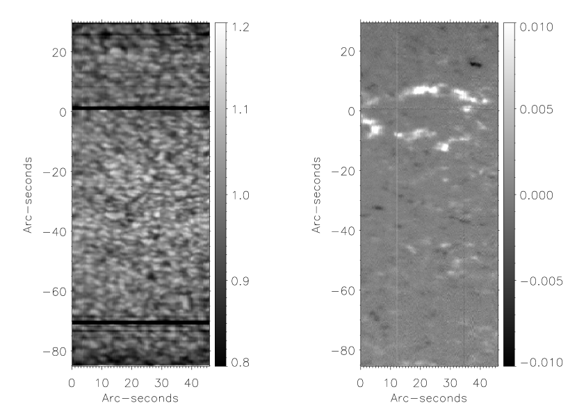
Figure 1: Continuum intensity map (left) and reconstructed magnetogram (right) of the quiet Sun scan near 5250 Å. The magnetogram shows the integrated Stokes $V$ signal over a narrow bandwidth on the red lobe of the Fe I 5250.2 Å  line. In both panels, values are referred to the average quiet Sun intensity. The angular scale on the vertical axis measures the distance from the upper hairline.

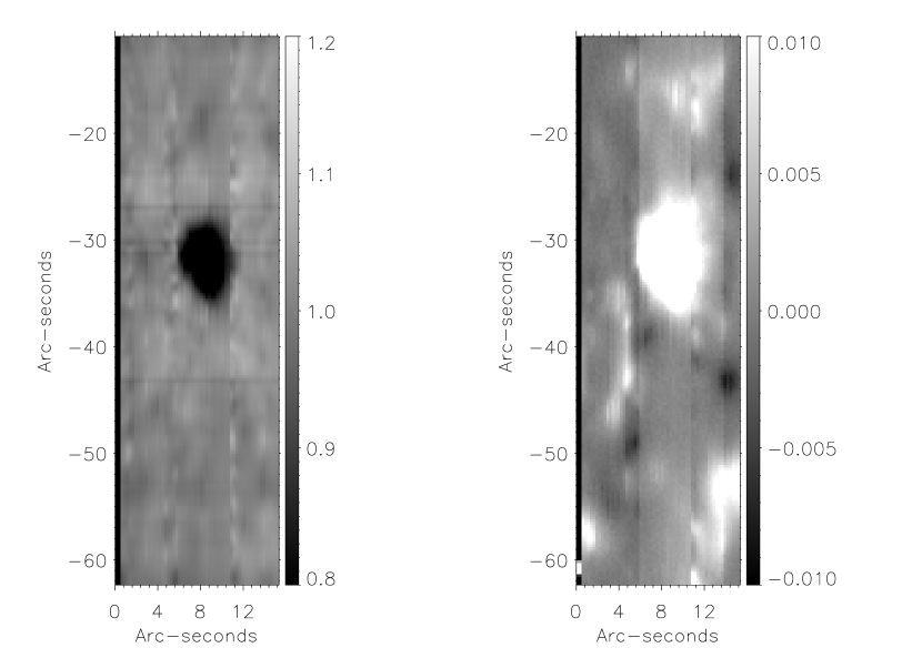
Figure 2: Continuum intensity map (left) and reconstructed magnetogram (right) of the pore scan near 5250 Å. The magnetogram shows the integrated Stokes $V$ signal over a narrow bandwidth on the red lobe of the Fe I 5250.2 Å  line. In both panels, values are referred to the average quiet Sun intensity. The angular scale on the vertical axis measures the distance from the upper hairline.

The first natural step in the analysis of these observations, before even considering any inversions, is to calculate the Stokes $V$ amplitude ratio of the Fe I line 5250.2 to 5247.0 Å  (hereafter, the line ratio). One would expect to obtain a rough idea of the intrinsic magnetic field strength from this value alone. A simple calibration was derived by taking the thermal stratification of the Harvard-Smithsonian Reference Atmosphere (HSRA, see Gingerich et al. 1971) and adding random (depth-independent) Gaussian temperature perturbations with an amplitude (standard deviation) of $\pm$300 K, different magnetic field strengths and a fixed macroturbulence of 3 km s^-1 (this value corresponds roughly to our spectral resolution). Line-of-sight gradients of temperature, field strength and velocity are also included. Figure 3 shows the line ratio obtained from the synthetic profiles as a function of the magnetic field employed to synthesize them. The line ratio is computed simply as the peak-to-peak amplitude ratio of the Stokes $V$ profiles. Notice that when the same experiment is carried out with a variable macroturbulent velocity the scatter increases considerably, even for relatively small values of up to 1 km s^-1 (right panel). The syntheses of Fig 3 consider the partial blends of all 6 lines in the 5250 Å  spectral range.

Figure 3: Line ratio calibration using synthetic Stokes profiles of Fe I 5250 Å emergent from the HSRA model atmosphere after adding random temperature perturbations and magnetic fields. Left: Macroturbulence was kept fixed at 3 km s^-1. Right: Random macroturbulence varies between 0 and 1 km s^-1.

Figure 4 shows the observed line ratios for both scans. According to our calibration (see above), ratios close to 1 indicate strong fields of nearly (at least) $\sim$2 kG, whereas larger values would suggest the presence of weaker fields, down to the weak-field saturation regime at (at most) $\sim$500 G corresponding to a ratio of 1.5. Figure 4 is somewhat disconcerting at first sight. The pore exhibits the expected behavior with strong $\sim$2 kG fields at the center that decrease gradually towards the outer boundaries until it becomes weak. The network and plage patches, on the other hand, contain relatively large areas with high ratios of 1.4 and even 1.6 at some locations. This is in sharp contrast with the strong fields ($\sim$1.5 kG) that one would expect in network and plage regions (e.g., Stenflo et al. 1984; Sánchez Almeida & Lites 2000; Bellot Rubio et al. 2000).

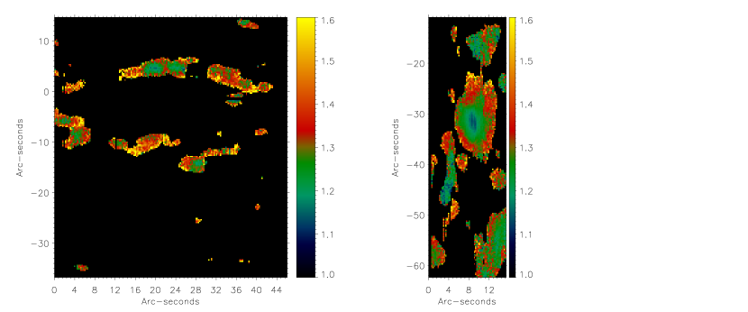
Figure 4: Amplitude ratio of Stokes $V$ in Fe I 5250.2 to Fe I 5247.0 Å. Left: Network patches observed in the quiet Sun scan. Right: A small pore (centered on coordinates [10,-30] approximately) and surrounding plage. Ratios close to 1 are indicative of a strong field of nearly 2 kG. Ratios close to 1.6 correspond to the weak-field (up to $\sim$500 G) regime. Black areas exhibit a circular polarization amplitude smaller than 1% and have not been inverted.

In view of these results we carried out inversions of the Stokes $I$ and $V$ profiles of the spectral lines in the 5250 Å  region emergent from the pore. We used the code LILIA considering a single magnetic component with a constant magnetic field embedded in a (fixed) non-magnetic background, taken to be the average quiet Sun. The resulting field-ratio scatter plot is shown in Figure 5. Note that the scatter in this case is much larger than that obtained with the HSRA calibration above. It is important to point out that the line ratio depicted in the figure is that measured on the synthetic profiles. Therefore, the scatter cannot be ascribed to inaccuracies of the inversion. As a verification test we picked one of the models with kG fields that produced a line ratio of $\simeq$1.4 and synthesized the emergent profiles with a different code (SIR), obtaining the same ratio. We therefore conclude that, when the field is strong, many different atmospheres are able to produce similar line ratios if realistic thermodynamic fluctuations and turbulence are allowed in the model. For weak fields, the ratio tends to a value of $\simeq$1.5 without much fluctuations.

Figure 5: Line ratio calibration using synthetic Stokes profiles obtained in the inversion of the pore.

Accepting then that we could no longer rely on the line ratio of Fe I 5247.0 and 5250.2 Å  as an independent reference to verify the magnetic fields obtained with the 6302 Å  lines, we considered the result of inverting each spectral region separately. Figure 6 depicts the scatter plot obtained. At the center of the pore, where we have the strongest fields (right-hand side of the figure), there is a very good correlation between the results of both measurements. However, those points lay systematically below the diagonal of the plot. This may be explained by the different “formation heights” of the lines. The Fe I lines at 5250 Å  generally form somewhat higher than those at 6302 Å. If the field strength decreases with height, one would expect to retrieve a slightly lower field strength when using 5250 Å. Unfortunately, the correlation breaks down for the weaker fields. In Figure 7 we can see that both sets of lines yield approximately the same field strengths (with a slightly lower values for the 5250 inversions, as discussed above) for longitudinal fluxes above some $\sim$500 G. Below this limit our diagnosis is probably not sufficiently robust.

Figure 6: Intrinsic field strengths determined from inverting the lines at 5250 (ordinates) and 6302 (abscissa) observed in the pore. The solid line shows the diagonal of the plot.

Figure 7: Differences in intrinsic field strengths measured at 6302 and 5250 Å  as a function of the average longitudinal magnetic flux density. The solid line represents the median value over 100 G bins. The dashed lines represent the standard deviation of the points in each bin.

If instead of the intrinsic field we consider the longitudinal magnetic flux, we obtain a fairly good agreement between both spectral regions. The Milne-Eddington inversions with MELANIE yield a Pearsons correlation coefficient of 0.89. In principle, the agreement is somewhat worse for the LILIA inversions, with a correlation coefficient of 0.60. However, we have found that this is due to a few outlayer points. Removing them results in a correlation coefficient of 0.82.

The situation becomes more complicated in the network. The results of inverting a network patch with MELANIE and LILIA can be seen in Figure 8. The inversions with MELANIE (upper panels) do not agree very well with each other. The correlation coefficient is only 0.23. The 5250 Å  map (upper right panel in the figure) looks considerably more noisy and rather homogeneous, compared to the 6302 Å  map (upper left). The LILIA inversions (lower panels) exhibit somewhat better agreement (correlation is 0.65), but again look very noisy at 5250 Å.

Figure 8: Longitudinal flux density from the inversions of a network patch at 6302 (left) and 5250 Å  (right). Upper panels: Inversions with the Milne-Eddington code MELANIE. Lower panels: Inversions with the LTE code LILIA. Spatial scales are in pixels.

Figure 9 depicts average profiles over a network patch. The 5250 line ratio for this profile is 1.21. We started by exploring the uniqueness of the magnetic field strength inferred with the simplest algorithm, MELANIE. Each one of these average profiles was inverted 100 times with random initializations. The results are presented in Figures 10 and 11, which show the values obtained versus the goodness of the fit, defined as the merit function $\chi^{2}$, which in this work is defined as:

$$\chi^{2}={1\over N_{p}}\sum_{i=1}^{N_{p}}{(I_{i}^{obs}-I_{i}^{syn})^{2}\over\sigma_{i}^{2}}\,,$$ (1)

where $N_{p}$ is the number of wavelengths and $\sigma_{i}$ have been taken to be 10^-3, so that a value of $\chi^{2}$=1 would represent on average a good fit at the 10^-3 level. The average profiles inverted here have a much lower noise (near 10^-4) and thus it is some times possible to obtain $\chi^{2}$ smaller than 1.

The $\chi^{2}$ represented in the plots is the one corresponding to the Stokes $V$ profile only (although the inversion codes consider both $I$ and $V$, but $I$ is consistently well reproduced and does not help to discriminate among the different solutions). Most of the fits correspond to kG field, indicating that inversions of network profiles are very likely to yield high field strengths. However, there exists a very large spread of field strength values that provide reasonably good fits to the observed data. This is especially true for the 5250 Å  lines, for which it is possible to fit the observations virtually equally well with fields either weaker than 500 G or stronger than 1 kG. In the case of 6302 Å  the best solutions are packed around $\simeq$1.5 kG, although other solutions of a few hecto-Gauss (hG) are only slightly worse than the best fit.

Figure 9: Average observed Stokes $V$ profiles in a network patch (located approximately around coordinates [20,7] in Figure 1). Ordinate values are related to the average quiet Sun continuum intensity. The 5250 line ratio (the relevant Fe I lines are marked with arrows) is 1.21.

Figure 10: Representation of the solutions from 100 different inversions of the 5250 Å  region with random initializations obtained using the Milne-Eddington code MELANIE. The field strength inferred by the inversion is plotted versus the quality of the fit, as measured by the merit function $\chi^{2}$.

Figure 11: Representation of the solutions from 100 different inversions of the 6302 Å  region with random initializations obtained using the Milne-Eddington code MELANIE. The field strength inferred by the inversion is plotted versus the quality of the fit, as measured by the merit function $\chi^{2}$.

It could be argued that Milne-Eddington inversions are too simplistic to deal with network profiles, since they are known to exhibit fairly strong asymmetries (both in area and in amplitude) that cannot be reproduced by a Milne-Eddington model. With this consideration in mind, we made a similar experiment using the LILIA and SIR codes. Figures 12 and 13 show the results obtained with LILIA. The magnetic and non-magnetic atmospheres have been forced to have the same thermodynamics in order to reduce the possible degrees of freedom (on the downside, this introduces an implicit assumption on the solar atmosphere). Again, the 6302 Å  lines seem to yield somewhat more robust inversions. The best fits correspond to field strengths of approximately 1.5 kG, with weaker fields delivering somewhat lower fit quality. The 5250 Å  lines give nearly random results (although they tend to be clustered between 500 and 800 G there is a tail of good fits with up to almost 1400 G). Similar results are obtained using SIR. In order to give an idea of what the different $\chi^{2}$ values mean, we present some of the fits in Fig 14.

Figure 12: Representation of the solutions from 100 different inversions of the 5250 Å  region with random initializations obtained using the LTE code LILIA. The field strength inferred by the inversion is plotted versus the quality of the fit, as measured by the merit function $\chi^{2}$.

Figure 13: Representation of the solutions from 100 different inversions of the 6302 Å  region with random initializations obtained using the LTE code LILIA. The field strength inferred by the inversion is plotted versus the quality of the fit, as measured by the merit function $\chi^{2}$.

Figure 14: Fits obtained with MELANIE (left) and LILIA (right) to the average network profile observed at 5250 (upper four panels) and 6302 Å  (lower four panels). For each case we show the best fit (smaller $\chi^{2}$) and a not so good one.

The thermal stratifications obtained in the 6302 Å  inversions are relatively similar, although the weaker fields require a hotter upper photosphere than the stronger fields (see Fig 15). On the other hand, the 5250 Å  inversions do not exhibit a clear correlation between the magnetic fields and temperature inferred (Fig 16).

Figure 15: Temperature stratification of the models obtained from the 6302 Å  inversions with LILIA. Solid line: Models that include kG fields. Dashed line: Models with sub-kG field.

Figure 16: Temperature stratification of the models obtained from the 5250 Å  inversions with LILIA. Solid line: Models that include kG fields. Dashed line: Models with sub-kG field.

The MISMA code was also able to find good solutions with either weak or strong fields. The smallest $\chi^{2}$ values correspond systematically to kG fields, but there are also some reasonably good fits ($\chi^{2}\simeq 1$) obtained with weak fields of $\sim$500 G (Figs 17 and 18). However, we found that all the weak-field solutions for 6302 Å  have a temperature that increases outwards in the upper photosphere (Fig 17). This might be useful to discriminate between the various solutions. The 5250 Å  lines, on the other hand, do not exhibit this behavior (Fig 18).

Figure 17: Inversions of the 6302 Å  region. Average magnetic field in the lower photosphere of the MISMA component that harbors more flux, as a function of the quality of the fit $\chi^{2}$. Asterisks: Solutions where the temperature decreases outwards in the upper photosphere. Diamonds: Solutions where the temperature increases outwards in the upper photosphere.

Figure 18: Inversions of the 5250 Å  region. Average magnetic field in the lower photosphere of the MISMA component that harbors more flux, as a function of the quality of the fit $\chi^{2}$. Asterisks: Solutions where the temperature decreases outwards in the upper photosphere. Diamonds: Solutions where the temperature increases outwards in the upper photosphere.

In principle it would seem plausible to discard the models with outward increasing temperature using physical arguments. This would make us conclude from the 6302 Å  lines that the fields are actually very strong, between $\sim$1.5 and 2.5 kG (it would not be possible to draw similar conclusions from the 5250 Å  lines). In any case, it would be desirable to have a less model-dependent measurement that could be trusted regardless of what the thermal stratification is.

Interestingly, when we invert all four Fe I lines simultaneously, both at 5250 and 6302 Å, the weak-field solutions disappear from the low-$\chi^{2}$ region of the plot and the best solutions gather between approximately 1 and 1.4 kG (see Fig 19).

Figure 19: Inversions of combined 5250 and 6302 Å  profiles. Average magnetic field in the lower photosphere of the MISMA component that harbors more flux, as a function of the quality of the fit $\chi^{2}$.

Socas-Navarro et al. (2006a) present a list of spectral lines with identical excitation potentials and oscillator strengths. We decided to test one of the most promising pairs, namely the Fe I lines at 4122 and 9000 Å. The choice was made based on their equivalent widths, Landé factors and also being reasonably free of blends in the quiet solar spectrum. Simulations similar to those in Figure 3 showed that the line-ratio technique is still incapable of retrieving an unambiguous field strength due to the presence of line broadening. Also, even if the line opacities are the same, the continuum opacities are significantly different at such disparate wavelengths, but in any case the line opacity is much stronger than the background continuum where the Stokes $V$ lobes are formed.

When we tested the robustness of inversion codes applied to this pair of lines, we obtained extremely reliable results as described below. Unfortunately we do not have observations of these two lines and therefore resorted on synthetic profiles to perform the tests. We used a 2-component reference model, where both components have the thermal structure of HSRA. The magnetic comonent has an arbitrary magnetic field and line-of-sight velocity. The field has a linear gradient and goes from $\simeq$1.6 kG at the base of the photosphere to 1 kG at continuum optical depth $\log(\tau_{5000})$=-4. The velocity field goes from 2.5 km s^-1 to 0.4 km s^-1 at $\log(\tau_{5000})$=-4. The magnetic component has a filling factor of 0.2. The reference macroturbulence is 3 km s^-1, which is roughly the value inferred from our observations. The spectra produced by this model at 5250 and 6302 Å  are very similar to typical network profiles. We considered the reference 4122 and 9000 Å  profiles as simulated observations and inverted them with two different methods.

Figure 20: Inversions of the proposed Fe I 4122 and 9000 Å  profiles. Average magnetic field in the lower photosphere of the magnetic component as a function of the quality of the fit $\chi^{2}$.

In order to make the test as realistic as possible, we gave the inversion code a somewhat erroneous non-magnetic profile. Specifically, we multiplied the profile from the reference non-magnetic component by a factor of 0.9 and shifted it 1 pixel towards the red. The wavelength shift corresponds to roughly 0.36 km s^-1 in both regions. This distorted non-magnetic profile was given as input to the inversion codes. We inverted the reference profiles using LILIA with 100 different initializations. Only $\sim$30% of the inversions converged to a reasonably low value of $\chi^{2}$, with the results plotted in Figure 20. We can see that the inversions are extremely consistent over a range of $\chi^{2}$ much larger than in the previous cases. In fact, none of the solutions are compatible with weak fields, suggesting that these lines are much better at discriminating intrinsic field strengths.

A much more demanding verification for the diagnostic potential of these new lines is to use a simpler scenario in the inversion than in the synthesis of the reference profiles, incorporating typical uncertainties in the calculation. After all, the real Sun will always be more complex than our simplified physical models. Thus, inverting the reference profiles with the Milne-Eddington code is an appropriate test. For this experiment we not only supplied the same “distorted” non-magnetic profile as above, but we also introduced a systematic error in the $\log(gf)$ of the lines. We forced the opacity of the 9000 Å  line to be 20% lower than that of 4122 (instead of taking them to be identical, as their tabulated values would indicate). Again, we performed 100 different inversions of the reference set of profiles with random initializations. In this case the inversion results are astonishingly stable, with 98 out of the 100 inversions converging to a $\chi^{2}$ within 15% of the best fit. The single-valued magnetic field obtained for those 98 inversions has a median of 1780 G with a standard deviation of only 3 G. The small scatter does not reflect the systematic errors introduced by several factors, including: a)the inability of the Milne-Eddington model to reproduce the comparatively more complex referece profiles; b)the artificial error introduced in the atomic parameters of the 9000 Å  line; c)the distortion (scale and shift) of the non-magnetic profile provided to the inversion code.

A final caveat with this new pair is that, even though the synthetic atlas of Socas-Navarro et al. (2006a) indicates that the 9000 Å  line Stokes $V$ profile is relatively free of blends, this still needs to be confirmed by observations (there is a very prominent line nearby that may complicate the analysis otherwise).

5 Conclusions

The ratio of Stokes $V$ amplitudes at 5250 and 5247 Å  is a very good indicator of the intrinsic field strength in the absence of line broadening, e.g. due to turbulence. However, line broadening tends to smear out spectral features and reduce the Stokes $V$ amplitudes. This reduction is not the same for both lines, depending on the profile shape. If the broadening could somehow be held constant, one would obtain a line-ratio calibration with very low scatter. However, if the broadening is allowed to fluctuate, even with amplitudes as small as 1 km s^-1, the scatter becomes very large. Fluctuations in the thermal conditions of the atmosphere further complicate the analysis. This paper is not intended to question the historical merits of the line-ratio technique, which led researchers to learn that fields seen in the quiet Sun at low spatial resolution are mostly of kG strength with small filling factors. However, it is important to know its limitations. Otherwise, the interpretation of data such as those in Figure 4 could be misleading. Before this work, most of the authors were under the impression that measuring the line ratio of the 5250 Å  lines would always provide an accurate determination of the intrinsic field strength.

With very high-resolution observations, such as those expected from the Advanced Technology Solar Telescope (ATST, Keil et al. 2003) or the Hinode satellite, there is some hope that most of the turbulent velocity fields may be resolved. In that case, the turbulent broadening would be negligible and the line-ratio technique would be more robust. However, even with the highest possible spatial resolution, velocity and temperature fluctuations along the line of sight will still produce turbulent broadening.

From the study presented here we conclude that, away from active region flux concentrations, it is not straightforward to measure intrinsic field strengths from either 5250 or 6302 Å  observations taken separately. Weak-flux internetwork observations would be even more challenging, as demonstrated recently by Martínez González (2007). Surprisingly enough, the 6302 Å  pair of Fe I lines is more robust than the 5250 Å  lines in the sense that it is indeed possible to discriminate between weak and strong field solutions if one is able to rule out a thermal stratification with temperatures that increase outwards. Even so, this is only possible when one employs an inversion code that has sufficient MHD constrains (an example is the MISMA implementation used here) to reduce the space of possible solutions.

The longitudinal flux density obtained from inversions of the 6302 Å  lines is better determined than those obtained with 5250 Å. This happens regardless of the inversion method employed, although using a code like LILIA provides better results than a simpler one such as MELANIE. The best fits to average network profiles correspond to strong kG fields, as one would expect.

An interesting conclusion of this study is that it is possible to obtain reliable results by inverting simultaneous observations at both 5250 and 6302 Å. Obviously this would be possible with relatively sophisticated algorithms (e.g., LTE inversions) but not with simple Milne-Eddington inversions.

The combination of two other Fe I lines, namely those at 4122 and 9000 Å, seems to provide a much more robust determination of the quiet Sun magnetic fields. Unfortunately, these lines are very distant in wavelength and few spectro-polarimeters are capable of observing them simultaneously. Examples of instrument with this capability are the currently operational SPINOR and THEMIS, as well as the planned ATST and GREGOR. Depending on the evolution time scales of the structures analyzed it may be possible for some other instruments to observe the blue and red lines alternatively.

References

- Bellot Rubio et al. (2000) Bellot Rubio, L. R., Ruiz Cobo, B., & Collados, M. 2000, ApJ, 535, 475
- Domínguez Cerdeña et al. (2003) Domínguez Cerdeña, I., Sánchez Almeida, J., & Kneer, F. 2003, A&A, 407, 741
- Domínguez Cerdeña et al. (2006) Domínguez Cerdeña, I., Sánchez Almeida, J., & Kneer, F. 2006, ApJ, 646, 1421
- Elmore et al. (1992) Elmore, D. F., Lites, B. W., Tomczyk, S., Skumanich, A., Dunn, R. B., , Schuenke, J. A., Streander, K. V., Leach, T. W., Chambellan, C. W., Hull, & Lacey, L. B. 1992, in Proc SPIE, Vol. 1746, 22
- Gingerich et al. (1971) Gingerich, O., Noyes, R. W., Kalkofen, W., & Cuny, Y. 1971, Sol. Phys., 18, 347
- Keil et al. (2003) Keil, S. L., Rimmele, T., Keller, C. U., Hill, F., Radick, R. R., Oschmann, J. M., Warner, M., Dalrymple, N. E., Briggs, J., Hegwer, S. L., & Ren, D. 2003, in Innovative Telescopes and Instrumentation for Solar Astrophysics. Edited by Stephen L. Keil, Sergey V. Avakyan . Proceedings of the SPIE, Volume 4853, pp. 240-251 (2003)., 240–251
- Khomenko et al. (2003) Khomenko, E. V., Collados, M., Solanki, S. K., Lagg, A., & Trujillo Bueno, J. 2003, A&A, 408, 1115
- López Ariste et al. (2002) López Ariste, A., Tomczyk, S., & Casini, R. 2002, ApJ, 580, 519
- Lin & Rimmele (1999) Lin, H., & Rimmele, T. 1999, ApJ, 514, 448
- Martínez González et al. (2006) Martínez González, M., Collados, M., & Ruiz Cobo, B. 2006, A&A, in press
- Martínez González (2007) Martínez González, M. J. 2007, Memorie della Societa Astronomica Italiana, 78, 59
- Ren et al. (2003) Ren, D., Hegwer, S. L., Rimmele, T., Didkovsky, L. V., & Goode, P. R. 2003, in Innovative Telescopes and Instrumentation for Solar Astrophysics. Edited by Stephen L. Keil, Sergey V. Avakyan . Proceedings of the SPIE, Volume 4853, pp. 593-599 (2003)., 593–599
- Ruiz Cobo & del Toro Iniesta (1992) Ruiz Cobo, B., & del Toro Iniesta, J. C. 1992, ApJ, 398, 375
- Sánchez Almeida (1997) Sánchez Almeida, J. 1997, ApJ, 491, 993
- Sánchez Almeida & Lites (2000) Sánchez Almeida, J., & Lites, B. W. 2000, ApJ, 532, 1215
- Skumanich & Lites (1987) Skumanich, A., & Lites, B. W. 1987, ApJ, 322, 473
- Socas-Navarro (2001) Socas-Navarro, H. 2001, in ASP Conf. Ser. 236: Advanced Solar Polarimetry – Theory, Observation, and Instrumentation, 487