Fine tuning of quantum operations performed via Raman transitions

Abstract

A scheme for fine tuning of quantum operations to improve their performance is proposed. A quantum system in $\Lambda$ configuration with two-photon Raman transitions is considered without adiabatic elimination of the excited (intermediate) state. Conditional dynamics of the system is studied with focus on improving fidelity of quantum operations. In particular, the $\pi$ pulse and $\pi/2$ pulse quantum operations are considered. The dressed states for the atom-field system, with an atom driven on one transition by a classical field and on the other by a quantum cavity field, are found. A discrete set of detunings is given for which high fidelity of desired states is achieved. Analytical solutions for the quantum state amplitudes are found in the first order perturbation theory with respect to the cavity damping rate $\kappa$ and the spontaneous emission rate $\gamma$. Numerical solutions for higher values of $\kappa$ and $\gamma$ indicate a stabilizing role of spontaneous emission in the $\pi$ and $\pi/2$ pulse quantum operations. The idea can also be applied for excitation pulses of different shapes.

I Introduction

An atomic $\Lambda$ system with Zeeman sublevels of the ground state, which are sufficiently long lived to store qubits, plays a very important role in quantum computations. Superpositions of such states can store quantum information for sufficiently long time to make various quantum algorithms feasible Langer et al. (2005). Therefore, researchers frequently consider such states in their proposals Parkins et al. (1993); Pellizzari et al. (1995); Bose et al. (1999); Beige et al. (2000); Chimczak (2005); Lim et al. (2006); Yuan and Zhu (2007) and use them in their experiments Riebe et al. (2004); Barrett et al. (2004); McKeever et al. (2004); Boozer et al. (2007); Legero et al. (2004); Hijlkema et al. (2007). Access to a good quantum memory is necessary, but not sufficient, to realize quantum computation. It is also important to be able to perform quantum operations on such coded qubits with high fidelity differing from unity by $10^{-5}$ or less Preskill (1998); Steane (1999).

Although there is no direct, strong coupling between the Zeeman sublevels, one can efficiently manipulate populations of the states using the two-photon Raman transition involving an auxiliary level, for example, state $|2\rangle$ in the $\Lambda$ configuration, as shown in Fig. 1. This method of qubit encoding and manipulation has many different implementations. There are single atoms or ions modeled by different level configuration systems: a three-level $\Lambda$ system Legero et al. (2004); Boozer et al. (2007), a four-level system with three levels in $\Lambda$ configuration, and one additional long-lived level, which does not participate in the transition van Enk et al. (1997); Pachos and Walther (2002), a six-level double $\Lambda$ system, which consists of two $\Lambda$ systems behaving exactly in parallel Pellizzari et al. (1995); Lim et al. (2006); Schön et al. (2007). There are also solid-state implementations: quantum dots modeled by the $\Lambda$-type Kiraz et al. (2004); Djuric and Search (2007) three-level system and superconducting quantum interference devices modeled by the $\Lambda$-type three-level system Zhou et al. (2002); Amin et al. (2003); Yang et al. (2003); Yang and Han (2004); Yang et al. (2004). In all these systems it is easy to store qubits and it is easy to perform single qubit gates just by turning the lasers on and off, to drive transitions for a proper period of time. Moreover, $\Lambda$-type systems are also perfect to realize the multiple qubit gates, as for example the crucial for quantum computation controlled NOT gate Beige et al. (2000); Tregenna et al. (2002); Goto and Ichimura (2004), because one can place two or more such systems in a microcavity and couple one transition in each $\Lambda$-type structure to the cavity field mode. Then, qubit interactions are mediated by the cavity field mode. Another way to realize two qubit gates is to perform the joint detection of photons leaking out of two separate cavities with trapped $\Lambda$-type systems Lim et al. (2006).

Since there are many advantages of devices composed of $\Lambda$-type systems and cavities, such systems are very popular elements of various quantum information processing schemes. However, there is one important drawback of such schemes — the population transferred to the intermediate level diminishes the fidelity of quantum operations performed with them. To avoid the destructive effect of populating the intermediate level, one can decide to work in the decoherence-free space Pellizzari et al. (1995); Goto and Ichimura (2004); Beige et al. (2000); Tregenna et al. (2002); Kis and Renzoni (2002); Sangouard et al. (2005) or, alternatively, one can assume that the cavity mode and the laser fields are far detuned from their respective transitions, as to make the population of the intermediate state negligible. The latter approach is referred to as adiabatic elimination. In realistic situations with not extremely large values of detunings, the population of the intermediate level is small but noticeable enough to significantly deteriorate the quality of quantum operations.

Figure 1: $\Lambda$-type Raman transition: a key ingredient of different quantum devices.

In this paper, we propose a scheme for fine tuning of the quantum operations performed via Raman transitions in the atomic $\Lambda$ system driven on one transition by a classical field, and on the other by a quantum cavity field. We discuss the conditional evolution of the $\Lambda$ system in a situation when the adiabatic elimination is not made, and we show that it is possible to take advantage of the fact that the intermediate state population oscillates rapidly, periodically approaching zero, which can be used to improve the quality of quantum gates based on the Raman transitions in the $\Lambda$ system. It turns out that it is possible, by setting appropriate values for the detuning, to make the population of the intermediate state negligible at the time the quantum operation is completed, and in this way we are able to increase significantly the fidelity of the operation. Such fine tuning of the quantum operations works well even for small detunings and, therefore, it can prove useful when one wants to perform quantum operations with high fidelity. We have found a discrete set of detunings for which perfect operations are possible if there is no damping. We have also found approximate analytical solutions describing the evolution of the $\Lambda$ system including both the cavity damping and spontaneous emission. Numerical results for higher values of the cavity decay rate and spontaneous emission rate show, somewhat unexpectedly, that the spontaneous emission can play a stabilizing role improving the result of quantum operation when the cavity decay rate becomes sufficiently large. We shortly address the issue of fine tuning for the nonrectangular pulses.

II Model

Let us consider two basic operations, which can be performed on qubit-encoding states of the $\Lambda$-type level structures: the $\pi$ pulse operation and the $\pi/2$ pulse operation. These two basic operations can be used to realize a number of important quantum information tasks as, for example, generation of maximally entangled states Chimczak (2005), quantum information transfer Bose et al. (1999); Chimczak et al. (2005), or the performing of controlled two qubit gates Lim et al. (2006). We consider an atom in $\Lambda$ configuration trapped in a cavity. The long-lived states $|0\rangle$ and $|1\rangle$ of the atom are coupled via the intermediate level $|2\rangle$ (see Fig. 1). The $|0\rangle\leftrightarrow|2\rangle$ transition is coupled to the cavity mode with a frequency $\omega_{\textrm{cav}}$ and coupling strength $g$. The second transition is driven by a classical laser field with the coupling strength $\Omega$. The frequency of the laser field is $\omega_{\textrm{L}}$. Both the classical laser field and the quantized cavity mode are detuned from the corresponding transition frequencies by $\Delta=(E_{2}-E_{1})/\hbar-\omega_{L}$. The population transfer between long-lived states $|0\rangle$ and $|1\rangle$ take place only when both transitions $|0\rangle\leftrightarrow|2\rangle$ and $|1\rangle\leftrightarrow|2\rangle$ are driven. Therefore, the qubit is safe if the laser is turned off. If we want to perform the $\pi$ pulse operation or the $\pi/2$ pulse operation then all we need to do is turning the laser on for a proper period of time.

The evolution of the $\Lambda$-type quantum systems is determined by the effective non-Hermitian Hamiltonian (we set $\hbar=1$ here and in the following):

$$H=(\Delta-i\gamma)\sigma_{22}+(\Omega\sigma_{21}+ga\sigma_{20}+{\rm{H.c.}})-i\kappa a^{\dagger}a\,,$$ (1)

where $\gamma$ is the spontaneous emission rate from the atomic state $|2\rangle$, and $\kappa$ is the cavity decay rate. In expression (1) we also introduce the flip operators $\sigma_{ij}=|i\rangle\langle j|$, where $i,j=0,1,2$. The effective Hamiltonian (1) describes conditional evolution of the atom-field system and will be used in our further calculations.

III Exact solutions

As a first step, we find the solutions for the Schrödinger equation when both $\gamma$ and $\kappa$ are zeros. This assumption allows us to obtain exact solutions. The Hamiltonian (1) takes in this case the form

$$H=\Delta\sigma_{22}+(\Omega\sigma_{21}+ga\sigma_{20}+{\rm{H.c.}})\,,$$ (2)

and it can be easily diagonalized in the basis being the product states of the atomic states and the cavity field photon states. To give the expressions a more compact form, we denote by $|jn\rangle=|j\rangle\otimes|n\rangle$ a state of the system consisting of the atomic state $|j\rangle$ and the cavity field with $n$ photons. Diagonalizing Hamiltonian (2) in the basis $\{|1\,n\rangle,|0\,n+1\rangle,|2\,n\rangle\}$ leads to the dressed states energies Parkins et al. (1993)

$$\omega_{0}=0, \omega_{\pm}=\frac{1}{2}(\Delta\pm\Omega^{\prime})\,,$$ (3)

where

$$\Omega^{\prime}=\sqrt{\Delta^{2}+4g^{2}(n+1)+4\Omega^{2}},$$ (4)

and the dressed states

$$|\Psi_{0}\rangle = -\sin\vartheta|1\,n\rangle+\cos\vartheta|0\,n+1\rangle$$

$$|\Psi_{-}\rangle = -\sin\varphi\left[\cos\vartheta|1\,n\rangle+\sin\vartheta|0\,n+1\rangle\right]$$ (5)

$$+\cos\varphi|2\,n\rangle$$

$$|\Psi_{+}\rangle = \cos\varphi\left[\cos\vartheta|1\,n\rangle+\sin\vartheta|0\,n+1\rangle\right]$$

$$+\sin\varphi|2\,n\rangle\,.\$$

We have introduced the notation

$$\sin\vartheta=\frac{\tilde{g}}{\sqrt{1+\tilde{g}^{2}}}, \cos\vartheta=\frac{1}{\sqrt{1+\tilde{g}^{2}}}\,,$$ (6)

$$\sin\varphi=\sqrt{\frac{\Omega^{\prime}+\Delta}{2\Omega^{\prime}}}, \cos\varphi=\sqrt{\frac{\Omega^{\prime}-\Delta}{2\Omega^{\prime}}}\,,$$ (7)

where $\tilde{g}=g\sqrt{n+1}/\Omega$.

Initially, the cavity field mode is in a vacuum state and, therefore, we are especially interested in the time evolution of the $|10\rangle$ state, so we assume $n=0$. Knowing the evolution for the dressed states (III), we can write the exact expression for this evolution of the initial state $|10\rangle(t)$

$$\textrm{e}^{-iHt}|10\rangle=|10\rangle(t)=a(t)|10\rangle+b(t)|01\rangle+c(t)|20\rangle,$$ (8)

where

$$a(t) = \cos^{2}\vartheta\left[\tilde{g}^{2}+f_{+}(t)-\frac{\Delta}{\Omega^{\prime}}f_{-}(t)\right],$$

$$b(t) = \sin\vartheta\cos\vartheta\left[-1+f_{+}(t)-\frac{\Delta}{\Omega^{\prime}}f_{-}(t)\right],$$ (9)

$$c(t) = \frac{2\Omega}{\Omega^{\prime}}f_{-}(t),$$

and

$$f_{\pm}(t) = \frac{1}{2}\left(\textrm{e}^{-i\omega_{+}t}\pm\textrm{e}^{-i\omega_{-}t}\right)\,.$$ (10)

The perfect $\pi$ pulse operation, defined by $|10\rangle\to|01\rangle$, requires the condition $\tilde{g}=1$, which means $g=\Omega$ and, therefore, we restrict the following considerations to this case only. Then, we have $\cos\vartheta=\sin\vartheta=1/\sqrt{2}$, and expressions (III) take simpler form.

It is evident from (III) that the excited atomic state population shows oscillatory behavior. Since the qubit is coded into the lower states, the fidelity of quantum operations performed on the qubit is reduced when some amount of population is present in the intermediate level. To overcome this problem, the upper level is usually adiabatically eliminated by choosing the detuning so large as to make the intermediate state population negligible. There is, however, an important drawback of this approach — it is necessary to use very large values of the detuning to achieve fidelities of the quantum operations sufficient for quantum computation. It would require $\Delta/g>640$ to get the fidelity different from unity by amount smaller than $10^{-5}$. Such detunings lead to long operation times, which are very challenging for optical cavities.

Here, we propose a scheme for fine tuning the quantum operations by using the fact that, in an ideal case, the population of the excited state evolves periodically in time, periodically approaching zero. By quantum operation, we understand a unitary operation transforming a given initial state into another (desired) quantum state. The quantum operation is perfect if the desired state is produced with the fidelity equal to unity. The idea of fine tuning is to choose the operation time in a way as to complete the operation when the population of the intermediate state is zero. To achieve this goal, we choose the evolution time in such a way that $f_{-}(t=t_{k})=0$, which means

$$(\omega_{+}-\omega_{-})\,t_{k}=\Omega^{\prime}\,t_{k}=2\pi\,k, k=1,2,3\ldots,$$ (11)

and

$$f_{+}(t_{k})=\exp\left[i\frac{\epsilon}{2}(\Omega^{\prime}-|\Delta|)t_{k}\right]$$ (12)

with

$$\epsilon=\left\{\begin{array}[]{rl}1&\textrm{ if }\Delta\geq 0\\ -1&\textrm{ if }\Delta<0\end{array}\right.\,.$$ (15)

Let us now require that, beside the relation (11), the evolution time satisfies the relation

$$\frac{1}{2}(\Omega^{\prime}-|\Delta|)\,t_{k,l}=\frac{\pi}{2}\,l,\quad l=1,2,3,\ldots,2k-1\,.$$ (16)

Both requirements for the evolution time can be satisfied provided the numbers $k$ and $l$ obey the relation

$$\frac{2k}{l}=\frac{\Omega^{\prime}}{\Omega^{\prime}-|\Delta|}\geq 1, 2k\geq l,$$ (17)

which leads to the discrete set of detunings $\Delta_{k,l}$ given by the formula

$$\left(\frac{\Delta_{k,l}}{2g}\right)^{2}=\frac{2\left(\frac{2k}{l}-1\right)^{2}}{2\left(\frac{2k}{l}-1\right)+1}\,.$$ (18)

For large detunings $2k/l-1$ is large, and we can drop unity in the denominator getting simpler, but approximate, relation. The discrete values of the detuning $\Delta_{k,l}$, in units of $2g$, are shown in Fig. 2

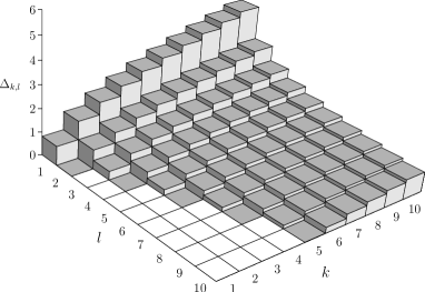
Figure 2: Discrete values of $|\Delta_{k,l}|$ (in units of 2$g$) for initial values of $k$ and $l$.

Enforcing both condition (11) and (16) gives us a discrete set of the evolution times for which solution (8) takes the form

$$|10\rangle(t_{k,l})=\frac{1}{2}\left[1+(i\epsilon)^{l}\right]|10\rangle-\frac{1}{2}\left[1-(i\epsilon)^{l}\right]|01\rangle\,.$$ (19)

The solution (19) is quite simple, and under appropriate choice of the numbers $\{k,l\}$ it gives either the superposition of the two initial states or one of the initial states.

The important $\pi$ operation we get for times

$$t_{\pi}=t_{k,l}, \textrm{ for }l\textrm{ even, }\quad l/2\textrm{ odd }$$ (20)

for which

$$\textrm{e}^{-iHt_{\pi}}|10\rangle = -|01\rangle\,.$$ (21)

For the second basic operation, the $\pi/2$ pulse operation, we should choose $l$ odd, for which we have

$$t_{\pi/2}=t_{k,l}, \textrm{ for }l\textrm{ odd, }$$ (22)

and the solutions are

$$\textrm{e}^{-iHt_{\pi/2}}|10\rangle=\left\{\begin{array}[]{ll}\frac{1-i\epsilon}{2}|10\rangle-\frac{1+i\epsilon}{2}|01\rangle,&\frac{l-1}{2}\textrm{ odd }\\[6.0pt] \frac{1+i\epsilon}{2}|10\rangle-\frac{1-i\epsilon}{2}|01\rangle,&\frac{l-1}{2}\textrm{ even }\end{array}\right.\,.$$ (23)

Depending on the value of $(l-1)/2$, we get from (23) one of the two orthogonal superposition states, which are maximally entangled (Bell states) of the atom-cavity system.

The solutions presented above are a direct consequence of the periodic evolution of the system. The periodicity appears when the two frequencies $\omega_{\pm}$, given by (3), are commensurate, i.e., their ratio is a ratio of integers. Taking absolute values of the two frequencies we can distinguish between the “fast” $\omega_{>}$ and “slow” $\omega_{<}$ frequency, where

$$\omega_{>\atop<}=\frac{1}{2}\left(\Omega^{\prime}\pm|\Delta_{k,l}|\right)=\left\{\begin{array}[]{ll}|\omega_{\pm}|&\textrm{ if }\Delta_{k,l}>0\\ |\omega_{\mp}|&\textrm{ if }\Delta_{k,l}<0\end{array}\right.\,.$$ (26)

From (11) and (16) it is easy to check that the frequencies $\omega_{<}$, $\omega_{>}$, and $\Omega^{\prime}=\omega_{<}+\omega_{>}$ are all commensurate, so the evolution is periodic.

The period of the slow oscillation is equal to

$$T=\frac{2\pi}{\omega_{<}}=\frac{4\pi}{\Omega^{\prime}-|\Delta_{k,l}|}=4\,\frac{t_{k,l}}{l}\,,$$ (27)

and is related to the time $t_{k,l}$ for perfect quantum operation. The period of oscillation of the intermediate state population is given by

$$T^{\prime}=\frac{2\pi}{\Omega^{\prime}}=\frac{2\pi}{\omega_{<}}\frac{\omega_{<}}{\Omega^{\prime}}=T\frac{l}{4k}=\frac{t_{k,l}}{k}\,.$$ (28)

The subsequent minima in the intermediate state population are separated by $T^{\prime}$. If $4k/l$ is an integer the period of the system evolution is equal to $T$, and, simultaneously, it is equal to an integer multiple ($4k/l$) of the period $T^{\prime}$. When $4k/l$ is an irreducible fraction, the period of the system evolution is equal to $4kT^{\prime}=lT$, and if the fraction is reducible the period is reduced appropriately.

For example, choosing $k=1$ and $l=2$, we have $\Delta_{k,l}=0$ and the resulting state is, according to (21), $-|01\rangle$, which is, up to the phase, an illustration of the perfect $\pi$ pulse operation. The operation is completed at time $t_{k,l}=kT^{\prime}$ for which the population of the intermediate state is zero, so the fidelity of the operation is equal to one. Similarly, by choosing $k=1$ and $l=1$ we get, according to (23), the superposition state $(1+i)/2|01\rangle-(1-i)/2|10\rangle$ which is generated with the fidelity equal to one. This is a perfect $\pi/2$ pulse operation, and the detuning in this case is equal to $\Delta_{1,1}/(2g)=0.8165$.

The two examples illustrate the idea of fine tuning of the quantum operations: choose one of the discrete values of the detuning $\Delta_{k,l}$ and corresponding operation time $t_{k,l}$ to complete the operation at a time when the population of the intermediate state is zero.

IV Approximate solutions

So far we have discussed the ideal case, when there is no cavity decay, and the spontaneous emission from the atomic excited level is ignored. To make the system useful for quantum information processing it is necessary to have access to the quantum information stored in the system and the possibility of sending it over long distances. In the case of the quantum system under discussion it is possible, when one mirror of the cavity is partially transparent. Of course, transparency of the mirror leads to a damping of the cavity field mode. Moreover, spontaneous emission introduces damping to the atomic system which spoils the desirable results of quantum operations. Unfortunately, in the presence of damping in the system, it is not possible to get exact analytical solutions; therefore, we have to resort to some approximations. When the two decay rates $\kappa$ and $\gamma$ are small we can apply the perturbative methods to find the first order corrections to the dressed states energies as well as the state amplitudes.

The first order corrections to the dressed states energies lead to the following modifications:

$$\tilde{\omega}_{0}=\omega_{0}-i\kappa_{0}, \tilde{\omega}_{\pm}=\omega_{\pm}-i(\kappa_{\pm}+\gamma_{\pm})\,,$$ (29)

where the damping rates $\kappa_{0},\kappa_{\pm}$, and $\gamma_{\pm}$ are given by

$$\kappa_{0}=\frac{\kappa}{2},\quad\kappa_{\pm}=\frac{\kappa}{4}\left(1\mp d\right),\quad\gamma_{\pm}=\frac{\gamma}{2}(1\pm d)\,,$$ (30)

where $d=\Delta/\Omega^{\prime}$. The solution (8) for the conditional evolution of the state $|10\rangle$, according to the first order perturbation theory with respect to both $\kappa$ and $\gamma$, is given, under the assumption $\Omega=g$ ($\tilde{g}=1$), by the following formulas:

$$a(t) = \frac{1}{2}\left\{(1+i\,2\eta\,d)\,\textrm{e}^{-\kappa_{0}t}+(1-i\,2\eta\,d)\,\tilde{f}_{+}(t)\right.$$

$$\left.-\left[d-i\,\xi-i\,\eta\,(1+d^{2})\right]\tilde{f}_{-}(t)\right\}$$

$$b(t) = \frac{1}{2}\left\{-\textrm{e}^{-\kappa_{0}t}+\tilde{f}_{+}(t)-\left(d-i\,\xi\right)\,\tilde{f}_{-}(t)\right\}$$

$$c(t) = \frac{1}{\Theta}\left\{-i\,\frac{\eta}{2}\textrm{e}^{-\kappa_{0}t}+i\,\frac{\eta}{4}(1+d^{2})\,\tilde{f}_{+}(t)\right.$$ (31)

$$\left.+\left[1-i\,\left(\frac{\eta}{2}-\bar{\gamma}\right)\,d\right]\tilde{f}_{-}(t)\right\}\,,$$

where we have introduced the notation $\Theta=\Omega^{\prime}/(2g)$, $\bar{\gamma}=\gamma/\Omega^{\prime}$, $\bar{\kappa}=\kappa/\Omega^{\prime}$, $\eta=\bar{\kappa}\Theta^{2}$, and $\xi=\bar{\gamma}/\Theta^{2}$. Functions $\tilde{f}_{\pm}$ have the form (10) except that the frequencies $\omega_{\pm}$ are replaced by $\tilde{\omega}_{\pm}$ from (29).

The solution (IV) is valid as long as $\kappa$ and $\gamma$ are small. In fact, the real smallness parameters are $\eta$ and $\xi$, so we require that both $\eta\ll 1$ and $\xi\ll 1$. In deriving (IV) we also discarded terms proportional to the product $\kappa\gamma$. On the other hand, the solution (IV) is valid for any value of the detuning $\Delta$. This means that it allows also for the resonant case of the $\pi$ pulse operation, when $k=1,l=2$ and $\Delta_{1,2}=0$. The resonant case is usually not recommended because of the spontaneous emission from the intermediate level. What is usually done to minimize the effect of spontaneous emission is the adiabatic elimination of the excited level. This requires large values of the detuning $\Delta$. It is seen from (IV) that when $1/\Theta=2g/\Omega^{\prime}\ll 1$, the amplitude $c(t)$ of the excited level is small. Neglecting this amplitude by setting $c(t)=0$ is exactly what the adiabatic elimination is about.

However, when the rate of spontaneous emission is small with respect to $2g$, the approximate solution (IV) should describe properly the role of spontaneous emission. This will be discussed later.

IV.1 Adiabatic elimination

The standard procedure used to eliminate the influence of the exited atomic level on the result of quantum operation is the adiabatic elimination of the excited level. It is realized by taking large detunings of the fields from the atomic transition frequencies, which makes the population of the excited state very small, and, in consequence, the state is assumed not to take part in the evolution. Assuming that $1/\Theta=2g/\Omega^{\prime}\ll 1$, which means that $\Delta/(2g)\gg 1$ and the requirements for adiabatic elimination are met, we can eliminate the state $|20\rangle$ from the evolution by putting in equations (IV) $c(t)=0$. We should also put $\gamma=0$ ($\bar{\gamma}=0,\xi=0$) to get rid of the $\gamma$ dependence in the other amplitudes. For large detuning we can also put $|d|=1$. With all these substitutions we get the following solutions:

$$a(t) = \frac{1}{2}\,\textrm{e}^{-\kappa_{0}t}\left[1+2i\epsilon\eta+(1-2i\epsilon\eta)\textrm{e}^{i\epsilon\omega_{<}t}\right]$$

$$= \textrm{e}^{-\kappa_{0}t}\,\textrm{e}^{\frac{i}{2}\epsilon\omega_{<}t}\left[\cos\left(\frac{1}{2}\omega_{<}t\right)+2\eta\sin\left(\frac{1}{2}\omega_{<}t\right)\right]$$

$$b(t) = \frac{1}{2}\,\textrm{e}^{-\kappa_{0}t}\left(-1+\textrm{e}^{i\epsilon\omega_{<}t}\right)$$ (32)

$$= \textrm{e}^{-\kappa_{0}t}\,\textrm{e}^{\frac{i}{2}\epsilon\omega_{<}t}\left[i\epsilon\sin\left(\frac{1}{2}\omega_{<}t\right)\right]\,,$$

where now $\eta=\kappa|\Delta|/(4g^{2})$. From (IV.1), one can calculate the time for the $\pi$ pulse operation, which takes the form

$$t_{\pi}(\kappa)=t_{k,l}\left[1+\frac{2}{l}\left(1-\frac{2}{\pi}\arctan\frac{1}{2\eta}\right)\right]\,,$$ (33)

and similarly for the $\pi/2$ pulse operation

$$t_{\pi/2}(\kappa)=t_{k,l}\left[1-\frac{1}{l}\left(1-\frac{4}{\pi}\arctan\frac{1}{1-2\eta}\right)\right]\,.$$ (34)

For large detuning $\omega_{<}=2g^{2}/|\Delta|$, $2\eta=\kappa/\omega_{<}$, and formulas (33) and (34) are consistent with corresponding formulas obtained when the adiabatic elimination is performed at the Hamiltonian level Bose et al. (1999). To be precise, the consistency is up to terms linear in $\kappa$, because the solutions (IV), and consequently (IV.1), were obtained in the linear approximation with respect to $\kappa$ (or $\eta$), i.e., under assumption $\eta\ll 1$. As far as the linear approximation is valid, one can derive simplified formulas for the relative changes of the operation times, which take the form

$$\frac{t_{\pi}(\kappa)-t_{k,l}}{t_{k,l}} = \frac{8\eta}{l\pi}$$

$$\frac{t_{\pi/2}(\kappa)-t_{k,l}}{t_{k,l}} = \frac{4\eta}{l\pi}\,.$$ (35)

In the presence of damping the evolution is not unitary and the resulting state, under the condition that neither a photon from the cavity nor a spontaneous emission photon are registered, is given by

$$|\Psi(t)\rangle=\frac{|\tilde{\Psi}(t)\rangle}{\sqrt{\langle\tilde{\Psi}(t)|\tilde{\Psi}(t)\rangle}}\,,$$ (36)

where

$$|\tilde{\Psi}|(t)\rangle=\text{e}^{-iHt}|10\rangle$$ (37)

is the unnormalized, conditional quantum state generated with the effective Hamiltonian (1). The fidelity of the resulting state is equal to $|\langle\Psi(t)|10\rangle(t_{k,l})|^{2}$, where $|10\rangle(t_{k,l})$ is a desired state given by (19). The solutions (IV.1) are the amplitudes of the unnormalized state (37) and must be normalized when we calculate state (36) and the fidelity in the presence of damping. For simplicity we use the same notation for the normalized amplitudes $a,b,c$ as for the unnormalized.

It is well known that when damping is present in the system, the periodic behavior of the system is lost, and the maxima and minima are shifted. This is exactly what we observe here. The quantum states generated in the presence of damping are no longer the ideal states (21) or (23), but if $\kappa/(2g)\ll 1$, the fidelity of the states generated can be quite high. The best choice for $t_{k,l}$ is that with the smallest possible values of $l$.

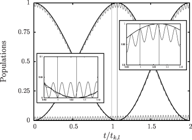
Figure 3: Comparison of the populations $|a(t)|^{2}$, $|b(t)|^{2}$, and $|c(t)|^{2}$ obtained from Eqs. (IV) and (IV.1) (normalized) for $k=31$, $l=2$, and $\kappa/(2g)=0.01$. Broad lines are populations after adiabatic elimination of the intermediate level. Vertical lines mark the times $t_{k,l}$ and $t_{\pi}(\kappa)$.

An example is shown in Fig. 3, where the $\pi$ pulse operation is illustrated. After adiabatic elimination of the intermediate level the populations of the remaining levels oscillate smoothly (broad lines), and the maximum is shifted from the time $t_{k,l}$ to $t_{\pi}(\kappa)$. However, without adiabatic elimination the populations are modulated with fast oscillations, and there are fast oscillations of the population of the intermediate level seen at the bottom. With the parameters of Fig. 3 the detuning $\Delta_{31,2}/(2g)=5.4321$. If $g/2\pi=16$ MHz then $\Delta_{31,2}/2\pi=173.83$ MHz, which is quite big, but the presence of the intermediate level is still visible, and it has significant influence on the fidelity of the resulting state. In the figures we illustrate the state evolution by plotting the state populations only, but the solutions are more general and give the state amplitudes that include also the phase information. The resulting state is a superposition of the basis states and the populations do not fully characterize the superposition. More precise characteristic of the state created during the evolution is its fidelity. To make it clear we give examples of the state amplitudes and the fidelities in Tables 1 and 2. For the example shown in Fig. 3, we present in Table 1 the amplitudes, calculated according to the approximate solution (IV), for the state amplitudes at different operation times.

Table 1: Normalized amplitudes of the quantum states for the $\pi$ pulse operation at various operation times ($k=31$, $l=2$, $\kappa/(2g)=0.01$)

Time	a	b	c	Fidelity
$t_{k,l}$	-0.0029+0.1078 i	-0.9940+0.0000 i	-0.0162-0.0098 i	0.9880
$t_{\pi}(\kappa)$	0.0022+0.0066 i	-0.9887-0.1012 i	0.0372+0.1043,i	0.9877
$t_{f}$	-0.0037+0.0064 i	-0.9946-0.1015 i	-0.0162-0.0133 i	0.9995

The time $t_{f}$, which we denote as the fine tuning time, is defined as the time at which the closest to $t_{\pi}(\kappa)$ maximum of the population of the state $|01\rangle$ (or minimum of the population of the state $|20\rangle$) occurs. From insets in Fig. 3 it is clear that $t_{f}=t_{k,l}+2T^{\prime}$, and this choice improves significantly the fidelity of the operation. Similar results are obtained for the $\pi/2$ pulse operation. An example is given in Table II, where the state amplitudes are presented for $k=31$, $l=1$, and $\kappa/(2g)=0.01$. In this case $\Delta_{31,1}/(2g)=7.7784$, and it is larger than in the previous case. This example is even more interesting because the fidelity at the operation time $t_{\pi/2}(\kappa)$ coming from the adiabatic elimination is smaller than the fidelity at time $t_{k,l}$ for ideal case of periodic evolution. The fine tuning, which this time gives $t_{f}=t_{k,l}+3T^{\prime}$, again improves the fidelity.

Table 2: Normalized amplitudes of the quantum states for the $\pi/2$ pulse operation at various operation times ($k=31$, $l=1$, $\kappa/(2g)=0.01$)

Time	a	b	c	Fidelity
$t_{k,l}$	0.5342+0.5351 i	-0.4623+0.4632 i	-0.0045+0.0029 i	0.9948
$t_{\pi/2}(\kappa)$	0.4584+0.5339 i	-0.5371+0.4497 i	0.0589-0.1034 i	0.9858
$t_{f}$	0.4632+0.5407 i	-0.5323+0.4579 i	-0.0058+0.0029 i	0.9999

From Fig. 3 it is clear that the time $t_{\pi}(\kappa)$ is different from the time $t_{k,l}$ for the ideal case. This difference suggests another possibility of fine tuning of the quantum operations, which consists in taking the operation time calculated from (33) as a new $t_{k,l}$ and adjust the detuning appropriately to get a maximum of the fast oscillations at the new $t_{k,l}$. Within linear approximation with respect to $\eta$ it leads to the detuning

$$|\Delta_{k,l}(\kappa)|=|\Delta_{k,l}|\left[1-\frac{4\eta}{l\pi}\sin^{2}\left(\frac{l\pi}{4}\right)\right].$$ (38)

By adjusting the detuning according to (38) we get the situation illustrated in Fig. 4.

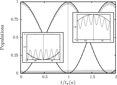
Figure 4: Same as Fig. 3, but with $\Delta_{k,l}(\kappa)$ given by (38). Vertical line marks the $t_{\pi}(\kappa)$.

Now, the fidelity at time $t_{\pi}(\kappa)$ takes the value $0.9992$. The fine tuning of the quantum operations can be performed in both ways: by finding the best operation time and/or adjusting the detuning. The values $\Delta_{k,l}$ given by (18) for the ideal case are a good starting point.

Examples given here show clearly that even for quite large values of detuning, the presence of the intermediate state is still visible, but the fidelity of the resulting states can be significantly enhanced when the operation time and/or the detuning are adjusted appropriately. This, however, requires knowledge of the solutions for the three-level system, and cannot be done when the adiabatic elimination of the intermediate state has already been accomplished.

Making the adiabatic elimination on the Hamiltonian level, consisting in diagonalizing the $2\times 2$ resulting Hamiltonian without resorting to perturbation theory, leads to the following results Bose et al. (1999):

$$a(t) = \textrm{e}^{\frac{i}{2}\left(\epsilon\omega_{<}+i\kappa\right)t}\left[\cos\left(\frac{1}{2}\,\omega_{<}(\kappa)t\right)\right.$$

$$\left.\hphantom{\textrm{e}^{\frac{i}{2}\left(\epsilon\omega_{<}+i\kappa\right)t}}+\frac{\kappa}{\omega_{<}(\kappa)}\sin\left(\frac{1}{2}\,\omega_{<}(\kappa)t\right)\right],$$

$$b(t) = \textrm{e}^{\frac{i}{2}\left(\epsilon\omega_{<}+i\kappa\right)t}\left[i\epsilon\frac{\omega_{<}}{\omega_{<}(\kappa)}\sin\left(\frac{1}{2}\,\omega_{<}(\kappa)t\right)\right],$$ (39)

where $\omega_{<}(\kappa)=\sqrt{\omega_{<}^{2}-\kappa^{2}}$ is the modified by $\kappa$ frequency $\omega_{<}$. Since the modification is at least quadratic in $\kappa$, by keeping only the linear terms in (IV.1), we easily reproduce formulas (IV.1). When corrections due to $\kappa^{2}$ become important, the populations of the two states oscillate with the modified frequency $\omega_{<}(\kappa)$ instead of $\omega_{<}$. The operation times are then given by

$$t_{\pi}(\kappa) = \frac{t_{k,l}}{r}\left[1+\frac{2}{l}\left(1-\frac{2}{\pi}\arctan\frac{r}{\sqrt{1-r^{2}}}\right)\right],$$

$$t_{\pi/2} = \frac{t_{k,l}}{r}\left[1-\frac{1}{l}\left(1-\frac{4}{\pi}\arctan\frac{r}{1-\sqrt{1-r^{2}}}\right)\right]\,\hskip 12.0pt$$ (40)

where $r$ is the ratio given by

$$r = \omega_{<}(\kappa)/\omega_{<}=\sqrt{1-(\kappa/\omega_{<})^{2}}.$$ (41)

Since $\omega_{<}=2g^{2}/|\Delta|$ decreases as $|\Delta|$ increases, the ratio $r$ for a given value of $\kappa$ can significantly differ from unity. This is true for very large detunings, i.e., for large values of $k$. It is important, however, to have $\kappa/\omega_{<}<1$, which puts some restrictions on the possible values of the detuning.

IV.2 Small detunings and spontaneous emission

In the case of small detunings, adiabatic elimination of the intermediate state is not possible, but solutions (IV) are valid for arbitrary detuning, that is, also for small detunings and resonant cases. In order to check how close to unity the fidelity of the $\pi$ pulse operation can be, we have investigated this problem for the parameters $(\Omega,g,\kappa)/2\pi=(16,16,0.05)$ MHz. This means that $\kappa/(2g)=0.0015$. Of course, for nonzero cavity damping $\kappa$, we should choose the smallest possible values for $l$ as to complete the operation in the shortest possible time. For example, for $k=1$, $l=2$ we get from (18) $\Delta_{k,l}=0$ and we obtain, after time $t_{k,l}$, the state $|01\rangle$ with the fidelity different from unity by less than $10^{-6}$. This is the resonant case, which is usually not recommended because of the spontaneous emission from the excited atomic state.

Similarly for the $\pi/2$ pulse operation, for $k=1$, $l=1$ we get $\Delta/(2g)=0.8165$, which means that for $g/2\pi=16$ MHz, $\Delta/2\pi=26.128$ MHz, and for such a value of $\Delta$ we can reproduce the state (23) with the fidelity that differs from unity by less than $10^{-6}$.

Choosing $k=4$ and $l=2$, we get the $\pi$ operation with $\Delta_{k,l}/(2g)=1.6036$ ($51.314$ MHz for $g/2\pi=16$ MHz), and we have a noticeable value of detuning. For $\kappa/2\pi=0.05$ MHz, we still get fidelity $0.99997$.

If spontaneous emission is ignored, one can expect very good performance of quantum operations at small detunings. The approximate formulas (IV) take into account spontaneous emission and they are valid whenever the spontaneous emission rate $\gamma$ is small with respect to $\Omega^{\prime}$. We can thus use equations (IV) to calculate the state amplitudes in the presence of spontaneous emission. Assuming the parameter values $(\Omega,g,\kappa,\gamma)/2\pi=(16,16,0.05,1)$ MHz, we have $\kappa/(2g)=0.0015$ and $\gamma/(2g)=0.03$ and, for $k=1$ and $l=2$, get the situation illustrated in Fig. 5,

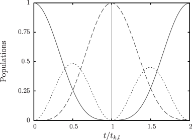
Figure 5: Evolution of the atom-field states populations (normalized): $|a(t)|^{2}$ (solid line), $|b(t)|^{2}$ (dashed line), $|c(t)|^{2}$ (dotted line) for $k=1$, $l=2$, $\kappa/(2g)=0.0015$, and $\gamma/(2g)=0.03$. Time is scaled in units of $t_{k,l}$.

where the state populations are shown. With these values of parameters the state $|01\rangle$ is generated with the fidelity still equal to $0.9989$, which is quite good. For the $\pi/2$ pulse operation the situation is even better and the fidelity takes the value $0.9993$. Of course, spontaneous emission rapidly deteriorates the quality of states generated at small detunings, but it is still possible to obtain remarkable fidelities.

V Numerical results

Approximate analytical results presented in previous section are valid only for sufficiently small values of $\kappa$ and $\gamma$. They illustrate the idea of fine tuning of quantum operations, but looking, for example, at Fig. 4, it is clear that it should be feasible to get even better results when more precise tuning is carried out. To this end, numerical calculations are necessary. The effective Hamiltonian (1) can be diagonalized numerically and we can find nonunitary evolution governed by this Hamiltonian. The numerical solution allows for adjustment of the detuning and corresponding time $t_{\pi}$ allowing for further improvement in the fidelity. For example, for the situation illustrated in Fig. 4, numerical optimization gives the fidelity $0.9997$ if we take $\Delta_{31,2}(\kappa)/(2g)=5.2409$ instead of $\Delta_{31,2}(\kappa)/(2g)=5.2380$ given by (38) and $\Delta_{31,2}/(2g)=5.4321$ given by (18), which for $g/2\pi=16$ MHz gives for the detunings $\Delta_{31,2}/2\pi$ values $167.71$, $167.62$, and $173.83$ MHz, respectively. This example shows that for $\kappa/(2g)=0.01$ and $\gamma=0$, analytical formulas give quite accurate results, and precise numerical tuning does improve the results but only slightly.

The situation changes dramatically when $\kappa$ and $\gamma$ are not so small as to justify linear approximation made in derivation of the analytical formulas. In such a situation the only reliable solutions are numerical solutions. To visualize the role of the two damping rates in the evolution we plot in Fig. 6 the populations of the quantum states for the value of $\kappa/(2g)=0.05$ and $\gamma=0$. The time $t_{\pi}(\kappa)$ is now calculated according to (IV.1). The amplitudes of the fast oscillation are quite big, and the $\pi$ pulse operation is far from being perfect. The detuning $\Delta_{31,2}$ is numerically tuned to fit the maximum of population and takes the value $\Delta_{31,2}/(2g)=4.4491$.

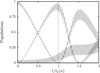
Figure 6: Numerical solutions for the state populations for $\kappa/(2g)=0.05$, $\gamma/(2g)=0$, and numerically tuned $\Delta_{31,2}/(2g)=4.4491$.

We find that the fidelity in this case is equal to $0.9660$ and is, of course, much worse than it was for $\kappa/(2g)=0.01$ shown in Fig. 4. In both cases the spontaneous emission is not taken into account. In Fig. 7 we present the same situation but when the spontaneous emission is included.

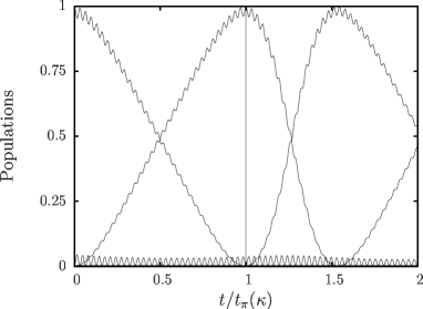
Figure 7: Same as Fig. 6 but for $\gamma/(2g)=0.03$

We take the value $\gamma/(2g)=0.03$ for the spontaneous emission rate, which gives for $g/2\pi=16$ MHz the value $\gamma/2\pi=1$ MHz. It turns out that the presence of spontaneous emission has a stabilizing effect on the evolution. The fast oscillations are damped significantly, and, surprisingly, the fidelity of the state generated becomes higher. For the parameters of Fig. 7 we find the fidelity $0.9994$. The reason for such behavior can be understood from Eq. (30), which shows the difference between $\kappa_{\pm}$ and $\gamma_{\pm}$ when the detuning is large and $|d|\rightarrow 1$. The two damping rates act in a sense in opposite directions: when fast oscillations are weakly damped by $\kappa$ they are strongly damped by $\gamma$, and vice versa. The effect is more pronounced for higher values of the detuning, i.e., for higher values of $k$. Similar effects can be observed for the $\pi/2$ pulse operation. These results show that in some situations spontaneous emission can play a positive role in performance of quantum operations.

V.1 Nonrectangular pulses

In real experiments the field cannot be switched on and off abruptly, so the rectangular pulses are rather not realistic. There are always a finite rise time and a finite fall time of the pulse. The pulse has definite shape, and usually what we observe in experiments depends on the pulse shape. Here, we address the effects of the pulse shape on the fine tuning discussed above.

With the Hamiltonian (1), assuming that $\Omega\to gF(t)$ and $g\to gF(t)$, where the function $F(t)$ describes the pulse shape, we get from the Schrödinger equation (units scaled to $2g$) the following set of equations for the state amplitudes

$$\dot{a}(t) = -\frac{i}{2}F(t)\,c(t)\,,$$

$$\dot{b}(t) = -\kappa\,b(t)-\frac{i}{2}F(t)\,c(t)\,,$$ (42)

$$\dot{c}(t) = -\frac{i}{2}F(t)\,a(t)-\frac{i}{2}F(t)\,b(t)-(\gamma+i\Delta)\,c(t)\,.$$

On resonance, without damping, the system (V.1) has the solutions

$$a(t) = \frac{1}{2}\left[1+f_{+}(t)\right]\,,$$

$$b(t) = \frac{1}{2}\left[-1+f_{+}(t)\right]\,,$$

$$c(t) = \frac{1}{\sqrt{2}}\,f_{-}(t)\,.$$ (43)

where

$$f_{\pm}(t) = \frac{1}{2}\left\{\exp\left[-\frac{i}{\sqrt{2}}\int_{0}^{t}F(t^{\prime})\text{d}t^{\prime}\right]\right.$$ (44)

$$\left.\pm\exp\left[\frac{i}{\sqrt{2}}\int_{0}^{t}F(t^{\prime})\text{d}t^{\prime}\right]\right\}\,.$$

The solutions (V.1) depend only on the pulse area $\int_{0}^{t}F(t^{\prime})\text{d}t^{\prime}$, so for any shape $F(t)$, with the same area, the resulting state after time $t$ is the same.

We do not know analytical solutions for the nonresonant case, even without damping, but the system (V.1) can be easily solved numerically for a given pulse shape $F(t)$. The solutions lack their periodic character and the quantum operation time depends on the pulse shape. The situation is thus more complex than for the rectangular pulses discussed in previous sections. Nevertheless, even in this case the idea of fine tuning is useful for finding the operation time. We illustrate the problem with few examples. Let us consider two different pulse shapes: the trapezium shape and the sine square shape, which are defined by the functions:

$$F(t)=\left\{\begin{array}[]{ll}s\frac{t}{t_{r}}&\text{ for }0<t<t_{r}\\ s&\text{ for }t_{r}<t<t_{p}-t_{f}\\ s\frac{t_{p}-t}{t_{f}}&\text{ for }t_{p}-t_{f}<t<t_{p}\end{array}\right.\,,$$ (48)

where

$$s=\frac{1}{1-\frac{t_{r}+t_{f}}{2t_{p}}}$$ (49)

is the scaling factor which makes the pulse area for the pulse duration $t_{p}$ to be the same as the area of the rectangular pulse of the same duration and unit height. The times $t_{r}$ and $t_{f}$ are the rise and fall time of the pulse, respectively. The normalization to the same pulse area ensures, on resonance, the same final state at time $t_{p}$ after the pulse for different pulse shapes.

The sine square pulse shape is given by the function (normalized to the same area)

$$F(t)=\left\{\begin{array}[]{ll}2\sin^{2}\left(\pi\frac{t}{t_{p}}\right)&\text{ for }0<t<t_{p}\\ 0&\text{ otherwise }\end{array}\right.\,.$$ (52)

The two pulse shapes are of different character. The trapezium is close to the rectangle when the rise and fall times are short. The sine square pulse is much narrower and changes smoothly over the whole duration time $t_{p}$. For the rectangle pulse we have $F(t)=1$.

To find approximately the proper operation times for pulse excitation, we use the following trick. We replace the oscillation frequency $\Omega^{\prime}$ of the intermediate state population with an “average frequency”

$$\Omega^{\prime}=\sqrt{\Delta^{2}+2}\to\Omega^{\prime}=\sqrt{\Delta^{2}+2\overline{F^{2}(t)}}\,,$$ (53)

where

$$\overline{F^{2}(t)}=\frac{1}{t_{p}}\int_{0}^{t_{p}}F^{2}(t)\,\text{d}t$$ (54)

which gives

$$\overline{F^{2}(t)}=\left\{\begin{array}[]{ll}s(4-s)/3&\text{ for trapezium}\\ 3/2&\text{ for sine square }\end{array}\right.\,,$$ (55)

with $s$ given by (49). Applying such a replacement we can calculate the “period” $T^{\prime}$ using (28) and the time $t_{k,l}$ for the considered operation using $\Delta_{k,l}$ defined by (18). The pulse is characterized by one parameter — the mean square amplitude defined by (54). For pulses with smooth rise and fall times, the evolution is no longer periodic, so the time $T^{\prime}$ is not really the period, but for small values of $l$ ($l=1,2$), the time $t_{k,l}$ calculated in this way is still a good approximation for the optimal operation time. It can at least be treated as a good starting point for further optimization.

To illustrate this situation we plot the evolution of the final states populations for two different pulse shapes. In Fig. 8 we present the evolution of final state populations for the trapezium shape with $t_{r}/t_{p}=t_{f}/t_{p}=0.1$ and the sine square pulse of the same duration. The other parameters are chosen as $k=3$, $l=2$, $\kappa=0$, $\gamma=0$, and the pulse duration $t_{p}=t_{k,l}$ with $t_{k,l}$ calculated with $\Omega^{\prime}$ adjusted according to (53).

Figure 8: Populations of the resulting states for pulse excitation with the trapezium pulse (upper figure) and sine square pulse (lower figure) for $k=3$, $l=2$, $\kappa=0$, and $\gamma=0$. The meaning of the lines is the same as in Fig. 5

The small value of $k=3$ gives the detuning $\Delta_{3,2}/(2g)=1.2649$ which is rather small, and in this case, as is seen from Fig. 8, the desired state is not of good quality. The fidelity, assuming the pulse duration $t_{p}=t_{k,l}$, is equal to $0.8176$ for the trapezium pulse and to $0.9529$ for the sine square pulse. This means that the approximation for $t_{k,l}$ is not very good for small detunings. Small detunings mean the situation is close to resonance, and the solutions should be close to periodic solutions (V.1). Actually, the oscillations are still visible in the figure. The fidelities of the generated states can be improved by adjusting the pulse duration. If the pulse duration is increased by a factor of $1.103$, for the trapezium pulse, we get the fidelity equal to $0.9681$, and this is the best result for the trapezium with $\Delta_{3,2}$. In the case of the sine square pulse, by increasing the pulse length by a factor of $1.087$, we get a fidelity better than $0.99999$. In this respect, for small detunings, the sine square pulse appears to be better than the trapezium pulse. We have to remember, however, that the results refer to the ideal situation, where there is no damping.

In Fig. 9 we illustrate the situation for $k=31$ and $l=2$.

Figure 9: Same as Fig. 8, but for $k=31$ and $l=2$.

In this case we have detuning $\Delta_{31,2}/(2g)=5.4321$, and the pulse duration time $t_{p}=t_{k,l}$ calculated according to the above procedure fits much better for producing desired state. The fidelities obtained with such $t_{p}$ are: $0.99994$ for the trapezium shape and $0.99899$ for the sine square pulse. The results are remarkable and confirm that the procedure works pretty well for larger detunings, i.e., higher values of $k$. The result for the trapezium pulse is optimal for the detuning $\Delta_{31,2}$, while the result for the sine square pulse can be still improved when the pulse duration $t_{k,l}$ is multiplied by a factor of $1.02$ giving a fidelity better than $0.99999$. Since the evolution is not periodic as it is in the case of rectangular pulses, the procedure will not work so well for higher values of $l$. The results obtained give evidence that for pulse excitation the idea of fine tuning of the quantum operations is also applicable.

In a real experimental situation, we have to take into account the damping rates $\kappa$ and $\gamma$. In analogy to the results for rectangular pulses, we can expect that the pulse duration should be increased to get desired states with good quality. The approximation described here does not give any hint as to how long the pulse should be, but starting from the ideal case it is easy to adjust the time numerically. For example, for the sine square pulse, taking $\kappa/(2g)=0.05$, $\gamma/(2g)=0.03$, and other parameters as in Fig. 9, we get a fidelity better than $0.99999$ for the time $1.154\,t_{k,l}$. Even in this case the approximate value of the pulse duration $t_{p}=t_{k,l}$ is a good starting point for numerical optimization.

VI Conclusion

In conclusion, we have studied the effect of the population of the intermediate state on two basic operations performed via the two-photon Raman transition in the atomic $\Lambda$ system. Full dynamics of the three-level system is taken into account without adiabatic elimination of the intermediate level. The dynamics studied are conditioned on no photon detection emitted by spontaneous emission and no photon detection leaking out of the cavity. We have found a discrete set of detunings leading to perfect $\pi$ pulse and $\pi/2$ pulse operations. It is shown how to make the population oscillations for improving the quantum operation precision useful. In the ideal case of $\kappa=0$ and $\gamma=0$, the population of the intermediate state $|2\rangle$ oscillates, becoming periodically zero and giving perfect operations. For nonzero, but small values of $\kappa$ and $\gamma$, the fidelity can achieve values very close to unity. Approximate analytical solutions obtained in first order perturbation theory are given, including both the cavity damping rate $\kappa$ as well as the spontaneous emission rate $\gamma$. Numerical results show that at certain circumstances, the spontaneous emission can play a positive, stabilizing role and improve the performance of quantum operations. The idea of fine tuning can also be applied for the pulse excitation with pulse shapes different than rectangle.

For realistic, moderate values of the detuning, the intermediate state has significant influence on the reliability of the quantum operation, but its destructive role can be limited by the fine tuning presented here. The possibility of using small or moderate values of detunings, without reducing the operation fidelity by the nonzero population of the excited state, is also important because the operation time is a function of the detuning, and short operation times are preferred to minimize effects of dissipation.

References

- Langer et al. (2005) C. Langer, R. Ozeri, J. D. Jost, J. Chiaverini, B. DeMarco, A. Ben-Kish, R. B. Blakestad, J. Britton, D. B. Hume, W. M. Itano, et al., Phys. Rev. Lett. 95, 060502 (2005).
- Pellizzari et al. (1995) T. Pellizzari, S. A. Gardiner, J. I. Cirac, and P. Zoller, Phys. Rev. Lett. 75, 3788 (1995).
- Bose et al. (1999) S. Bose, P. L. Knight, M. B. Plenio, and V. Vedral, Phys. Rev. Lett. 83, 5158 (1999).
- Beige et al. (2000) A. Beige, D. Braun, B. Tregenna, and P. L. Knight, Phys. Rev. Lett. 85, 1762 (2000).
- Chimczak (2005) G. Chimczak, Phys. Rev. A 71, 052305 (2005).
- Lim et al. (2006) Y. L. Lim, S. D. Barrett, A. Beige, P. Kok, and L. C. Kwek, Phys. Rev. A 73, 012304 (2006).
- Yuan and Zhu (2007) C.-H. Yuan and K.-D. Zhu, J. Phys. B 40, 801 (2007).
- Parkins et al. (1993) A. S. Parkins, P. Marte, P. Zoller, and H. J. Kimble, Phys. Rev. Lett. 71, 3095 (1993).
- Riebe et al. (2004) M. Riebe, H. Häffner, C. F. Roos, W. Hänsel, J. Benhelm, G. P. T. Lancaster, T. W. Körber, C. Becher, F. Schmidt-Kaler, D. F. V. James, et al., Nature (London) 429, 734 (2004).
- Barrett et al. (2004) M. D. Barrett, J. Chiaverini, T. Schaetz, J. Britton, W. M. Itano, J. D. Jost, E. Knill, C. Langer, D. Leibfried, R. Ozeri, et al., Nature (London) 429, 737 (2004).
- McKeever et al. (2004) J. McKeever, A. Boca, A. D. Boozer, R. Miller, J. R. Buck, A. Kuzmich, and H. J. Kimble, Science 303, 1992 (2004).
- Boozer et al. (2007) A. D. Boozer, A. Boca, R. Miller, T. E. Northup, and H. J. Kimble, Phys. Rev. Lett. 98, 193601 (2007).
- Legero et al. (2004) T. Legero, T. Wilk, M. Hennrich, G. Rempe, and A. Kuhn, Phys. Rev. Lett. 93, 070503 (2004).
- Hijlkema et al. (2007) M. Hijlkema, B. Weber, H. P. Specht, S. C. Webster, A. Kuhn, and G. Rempe, Nat. Phys. 3, 253 (2007).
- Preskill (1998) J. Preskill, Proc. R. Soc. London, Ser. A 454, 385 (1998).
- Steane (1999) A. M. Steane, Nature (London) 399, 124 (1999).
- van Enk et al. (1997) S. J. van Enk, J. I. Cirac, and P. Zoller, Phys. Rev. Lett. 78, 4293 (1997).
- Pachos and Walther (2002) J. Pachos and H. Walther, Phys. Rev. Lett. 89, 187903 (2002).
- Schön et al. (2007) C. Schön, K. Hammerer, M. M. Wolf, J. I. Cirac, and E. Solano, Phys. Rev. A 75, 032311 (2007).
- Kiraz et al. (2004) A. Kiraz, M. Atatüre, and A. Imamoḡlu, Phys. Rev. A 69, 032305 (2004).
- Djuric and Search (2007) I. Djuric and C. P. Search, Phys. Rev. B 75, 155307 (2007).
- Zhou et al. (2002) Z. Zhou, Shih-I. Chu, and S. Han, Phys. Rev. B 66, 054527 (2002).
- Amin et al. (2003) M. H. S. Amin, A. Y. Smirnov, and A. Maassen van den Brink, Phys. Rev. B 67, 100508(R) (2003).
- Yang et al. (2003) C.-P. Yang, Shih-I. Chu, and S. Han, Phys. Rev. A 67, 042311 (2003).
- Yang and Han (2004) C.-P. Yang and S. Han, Phys. Lett. A 321, 273 (2004).
- Yang et al. (2004) C.-P. Yang, Shih-I. Chu, and S. Han, Phys. Rev. Lett. 92, 117902 (2004).
- Tregenna et al. (2002) B. Tregenna, A. Beige, and P. L. Knight, Phys. Rev. A 65, 032305 (2002).
- Goto and Ichimura (2004) H. Goto and K. Ichimura, Phys. Rev. A 70, 012305 (2004).
- Kis and Renzoni (2002) Z. Kis and F. Renzoni, Phys. Rev. A 65, 032318 (2002).
- Sangouard et al. (2005) N. Sangouard, X. Lacour, S. Guérin, and H. R. Jauslin, Phys. Rev. A 72, 062309 (2005).
- Chimczak et al. (2005) G. Chimczak, R. Tanaś, and A. Miranowicz, Phys. Rev. A 71, 032316 (2005).