DFTT07/23

JINR-E2-2007-145

The arrow of time and the Weyl group:
all supergravity billiards are integrable^†
Pietro Fré^a and Alexander S. Sorin^b

^a Dipartimento di Fisica Teorica, Universitá di Torino,

$\&$ INFN - Sezione di Torino
via P. Giuria 1, I-10125 Torino, Italy

fre@to.infn.it

^b Bogoliubov Laboratory of Theoretical Physics,
Joint Institute for Nuclear Research,
141980 Dubna, Moscow Region, Russia

sorin@theor.jinr.ru

In this paper we show that all supergravity billiards corresponding to $\sigma$-models on any $\mathrm{U/H}$ non compact-symmetric space and obtained by compactifying supergravity to $D=3$ are fully integrable. The key point in establishing the integration algorithm is provided by an upper triangular embedding of the solvable Lie algebra associated with $\mathrm{U/H}$ into $\mathfrak{sl}(\mathrm{N},\mathbb{R})$ which always exists. In this context we establish a remarkable relation between the arrow of time and the properties of the Weyl group. The asymptotic states of the developing Universe are in one-to-one correspondence with the elements of the Weyl group which is a property of the Tits Satake universality classes and not of their single representatives. Furthermore the Weyl group admits a natural ordering in terms of $\ell_{T}$, the number of reflections with respect to the simple roots and the direction of time flows is always towards increasing $\ell_{T}$, which plays the unexpected role of an entropy.

 ^† This work is supported in part by the European Union RTN contract MRTN-CT-2004-005104 and by the Italian Ministry of University (MIUR) under contracts PRIN 2005-024045 and PRIN 2005-023102. Furthermore the work of A.S. was partially supported by the RFBR Grant No. 06-01-00627-a, RFBR-DFG Grant No. 06-02-04012-a, DFG Grant 436 RUS 113/669-3, the Program for Supporting Leading Scientific Schools (Grant No. NSh-5332.2006.2), and the Heisenberg-Landau Program.

1 Foreword

Notwithstanding its length and its somewhat pedagogical organization, the present one is a research article and not a review. All the presented material is, up to our knowledge, new. Due to the combination of several different mathematical results and techniques necessary to make our point, which is instead physical in spirit and relevant to basic questions in supergravity and superstring cosmology, we considered it appropriate to choose the present somewhat unconventional format for our paper. After the theoretical statement of our result, we have illustrated it with the detailed study of a few examples. These case-studies were essential for us in order to understand the main point which we have formalized in mathematical terms in part I and we think that they will be similarly essential for the physicist reader. The table of contents helps the reader to get a comprehensive view of the article and of its structure.

Contents

1. 1 Foreword
2. I Theory: Stating the principles
   1. 2 Supergravity billiards: a paradigm for cosmology
   2. 3 The paint group and the Tits Satake projection
      1. 3.1 The solvable algebra
      2. 3.2 The paint group and its Lie algebra
      3. 3.3 The subpaint group and the Tits Satake subalgebra
   3. 4 Triangular embedding in $\mathrm{SL(N,\mathbb{R})/SO(N)}$ and integrability
      1. 4.1 The integration algorithm for the Lax Equation
   4. 5 Properties of the general integral and the parameter space
      1. 5.1 Discussion of the generalized Weyl group
      2. 5.2 The arrow of time, trapped and critical surfaces
3. II Examples illustrating the principles
   1. 6 Choice of the examples
   2. 7 The simplest maximally split case: $\mathrm{SL(3,\mathbb{R})}/\mathrm{SO(3)}$
      1. 7.1 Discussion of the generalized Weyl group
      2. 7.2 The flow diagram and the critical surfaces for $\mathrm{SL(3,\mathbb{R})}$
   3. 8 The maximally split case $\mathrm{Sp(4,\mathbb{R})}/\mathrm{U(2)}$
      1. 8.1 The Weyl group and the generalized Weyl group of $\mathfrak{sp}(4,\mathbb{R})$
      2. 8.2 Construction of the $\mathfrak{sp}(4,\mathbb{R})$ Lie algebra
      3. 8.3 Parameterization of the compact group $\mathrm{U(2)}$ and critical submanifolds
      4. 8.4 Examples for $\mathfrak{sp}(4,\mathbb{R})$
         1. 8.4.1 An example of flow in the bulk of parameter space: $\Omega_{5}\,\Rightarrow\,\Omega_{8}$
         2. 8.4.2 An example of flow on the super-critical surface $\Sigma_{9}$: $\Omega_{6}\,\Rightarrow\,\Omega_{8}$
         3. 8.4.3 An example of flow on the super-critical surface $\Sigma_{2}$: $\Omega_{1}\,\Rightarrow\,\Omega_{8}$
   4. 9 The case of the $\mathfrak{so}(r,r+2s)$ algebra
      1. 9.1 The corresponding complex Lie algebra and root system
      2. 9.2 The real form $\mathfrak{so}(r,r+2s)$ of the $D_{r+s}$ Lie algebra
   5. 10 A case study for the Tits Satake projection: $\mathrm{SO(2,4)}$
      1. 10.1 The generalized Weyl group for $\mathrm{SO(2,4)}$
      2. 10.2 Vertices, edges and trapped surfaces
      3. 10.3 Examples of flows for $\mathrm{SO(2,4)}$
4. III Perspectives
   1. 11 Summary of results
   2. 12 Open problems and directions to be pursued

Part I Theory: Stating the principles

2 Supergravity billiards: a paradigm for cosmology

Cosmological implications of superstring theory have been under attentive consideration in the last few years from various viewpoints [1]. This involves the classification and the study of possible time-evolving string backgrounds which amounts to the construction, classification and analysis of supergravity solutions depending only on time or, more generally, on a low number of coordinates including time.

In this context a quite challenging and potentially highly relevant phenomenon for the overall interpretation of extra–dimensions and string dynamics is provided by the so named cosmic billiard phenomenon [2], [3], [4], [5]. This is based on the relation between the cosmological scale factors and the duality groups $\mathrm{U}$ of string theory. The group $\mathrm{U}$ appears as isometry group of the scalar manifold $\mathcal{M}_{scalar}$ emerging in compactifications of $10$–dimensional supergravity to lower dimensions $D<10$ and depends both on the geometry of the compact dimensions and on the number of preserved supersymmetries $\mathcal{N}_{Q}\leq 32$. For $\mathcal{N}_{Q}>8$ the scalar manifold is always a homogeneous space $\mathrm{U/H}$. The cosmological scale factors $a_{i}(t)$ associated with the various dimensions of supergravity are interpreted as exponentials of those scalar fields $h_{i}(t)$ which lie in the Cartan subalgebra of $\mathbb{U}$, while the other scalar fields in $\mathrm{U/H}$ correspond to positive roots $\alpha>0$ of the Lie algebra $\mathbb{U}$. The cosmological evolution is described by a fictitious ball that moves in the CSA of $\mathbb{U}$ and occasionally bounces on the hyperplanes orthogonal to the various roots: the billiard walls. Such bounces represent inversions in the time evolution of scale factors. Such a scenario was introduced by Damour, Henneaux, Julia and Nicolai in [2], [3], [4], [5], generalizing classical results obtained in the context of pure General Relativity [6]. In these papers the billiard phenomenon was mainly considered as an asymptotic regime near singularieties.

In a series of papers [7], [8, 9, 10] involving both the present authors and other collaborators it was started and developed what can be described as the smooth cosmic billiard programme. This amounts to the study of the billiard features within the framework of exact analytic solutions of supergravity rather than in asymptotic regimes. Crucial starting point in this programme was the observation [7] that the fundamental mathematical setup underlying the appearance of the billiard phenomenon is the so named Solvable Lie algebra parametrization of supergravity scalar manifolds, pioneered in [11] and later applied to the solution of a large variety of superstring/supergravity problems [12], [13], [16], [14], [15] (for a comprehensive review see [17]).

Thanks to the solvable parametrization, one can establish a precise algorithm to implement the following programme:

a

Reduce the original supergravity in higher dimensions $D\geq 4$ (for instance $D=10,11$) to a gravity-coupled $\sigma$–model in $D\leq 3$ where gravity is non–dynamical and can be eliminated. The target manifold is the non compact coset $\mathrm{U/H}\cong\exp\left[Solv\left(\mathrm{U/H}\right)\right]$ metrically equivalent to a solvable group manifold.

b

Utilize various group theoretical techniques in order to integrate analytically the $\sigma$–model equations.

c

Dimensionally oxide the solutions obtained in this way to extract time dependent solutions of $D\geq 4$ supergravity.

In view of the above observation we will use the following definition of supergravity billiards:

Definition 2.1

$<<$ A supergravity billiard is a one-dimensional $\sigma$-model whose target space is a non-compact coset manifold $\mathrm{U/H}$, metrically equivalent, in force of a general theorem, to a solvable group manifold $\exp\left[Solv\left(\mathrm{U/H}\right)\right]$. $>>$

There exists a complete classification [17, 18, 10] of all non-compact coset manifolds $\mathrm{U/H}$ relevant to the various instances of supergravities in all space-time dimensions $D$ and for all numbers $\mathcal{N}_{Q}$ of supercharges. A general important feature is that maximal supersymmetry $\mathcal{N}_{Q}=32$ corresponds to maximally split symmetric cosets.

Definition 2.2

$<<$ A symmetric coset manifold $\mathrm{U/H}$ is maximally split when the Lie algebra $\mathbb{U}$ of $\mathrm{U}$ is the maximally non compact real section of its own complexification and $\mathbb{H}\,\subset\,\mathbb{U}$ is the unique maximal compact subalgebra. In this case the Cartan subalgebra $\mathcal{C}$ is completely non-compact, namely the non-compact rank $r_{n.c.}=r$ equals the rank and the solvable Lie algebra $Solv\left(\mathrm{U/H}\right)$ is made by all the Cartan generators $\mathcal{H}_{i}$ plus the step operators $E^{\alpha}$ for all the positive roots $\alpha>0$. $>>$

In [19] the present authors shew that for maximally split cosets the one-dimensional $\sigma$-model is fully integrable and the general integral can be constructed using a well established algorithm endowed with a series of distinctive and quite inspiring features.

In the present paper we demonstrate that the algorithm of [19] can be actually extended to all the other cases, also those not maximally split, so that all supergravity billiards are in fact completely integrable as claimed in the title.

Besides demonstrating the integrability we will illustrate the main features of the general integral which reveal a very rich and highly interesting geometrical structure of the parameter space. In this context it will emerge a challenging new concept. The time flows appearing as exact analytical solutions of supergravity billiards have a preferred orientation which is intrinsically determined in group theoretical terms. There emerges a similarity between the second law of thermodynamics and the properties of cosmological evolutions just as there is such a similarity in the case of black-hole dynamics. We establish the following principle

Principle 2.1

$<<$ The asymptotic states of the cosmic billiard at past and future infinity $t=\pm\infty$ are in one-to-one correspondence with the elements $w_{i}$ of the duality algebra Weyl group $\mathrm{Weyl}(\mathbb{U})$. The Weyl group, which for suitable choice of $N$ is a subgroup of the symmetric group $\mathcal{S}_{N}$ admits a natural ordering in terms of the minimal number $\ell_{T}$ of reflections with respect to simple roots $\alpha_{i}$ necessary to reproduce any considered element $w$. The number $\ell_{T}(w)$, named the height of $w\in\mathrm{Weyl}(\mathrm{U})$, is the same as the number of transpositions of the corresponding permutation when $\mathrm{Weyl}(\mathrm{U})$ is embedded in the symmetric group. Time flows goes always in the direction of increasing $\ell_{T}$ which, therefore, plays the role of entropy. $>>$

3 The paint group and the Tits Satake projection

In [9] first and then more systematically in [18] it was observed that the Tits-Satake theory of non-compact cosets, which is a classical chapter of modern differential geometry, provides a natural frame to discuss the structure of the $\mathrm{U/H}$ cosets appearing in supergravity with particular reference to their role in billiard dynamics. In [9] a new concept was introduced, that of paint group, which plays a fundamental role in classifying the relevant $\mathrm{U/H}$ manifolds and grouping them into universality classes with respect to the Tits Satake projection. The systematics of these universality classes was developed in [18].

In the present paper we will clarify and illustrate by means of explicit examples the meaning of these universality classes showing that the essential features of billiard dynamics are just a property of the class, independently from the choice of the representative, namely independently from the choice of the paint group. In particular the Weyl group and the asymptotic states are common to the whole class. On the other hand the notion of the paint group enters in the precise definition of the parameter space for the general integral. Let us therefore recall the essential notions relevant to our subsequent discussion.

3.1 The solvable algebra

Following the discussion of [9] let us recall that in the case the scalar manifold of supergravity is a non maximally non-compact manifold $\mathrm{U/H}$ the Lie algebra $\mathbb{U}$ of the numerator group is some appropriate real form

$$\mathbb{U}\,=\,\mathbb{U}_{R}$$ (3.1)

of a complex Lie algebra $\mathbb{U}(\mathbb{C})$ of rank $r=\mbox{rank}(\mathbb{U})$. The Lie algebra $\mathbb{H}$ of the denominator $\mathrm{H}$ is the maximal compact subalgebra $\mathbb{H}\subset\mathbb{U}_{R}$, which has typically rank $r_{\rm c}<r$. Denoting, as usual, by $\mathbb{K}$ the orthogonal complement of $\mathbb{H}$ in $\mathbb{U}_{R}$

$$\mathbb{U}_{R}=\mathbb{H}\,\oplus\,\mathbb{K}$$ (3.2)

and defining as non-compact rank, or rank of the coset $\mathrm{U/H}$, the dimension of the noncompact Cartan subalgebra

$$r_{\rm nc}\,=\,\mbox{rank}\left(\mathrm{U/H}\right)\,\equiv\,\mbox{dim}\,\mathcal{H}^{\rm nc}\quad;\quad\mathcal{H}^{\rm nc}\,\equiv\,\mbox{CSA}_{\mathbb{U}(\mathbb{C})}\,\bigcap\,\mathbb{K}~{},$$ (3.3)

we obtain that $r_{\rm nc}<r$.

The manifold $\mathrm{U_{R}/H}$ is always metrically equivalent to a solvable group manifold $\mathcal{M}_{Solv}\equiv\exp[Solv(\mathrm{U_{R}/H})]$ although the form of the solvable Lie algebra $Solv(\mathrm{U_{R}/H})$, whose structure constants define the Nomizu connection, is more complicated when $r_{\rm nc}\,<\,r$ than in the maximally split case $r_{\rm nc}\,=\,r$. For the details on the construction of the solvable Lie algebra we refer to the literature [11, 17]. The important thing in our present context is that it exists. Furthermore, using a general theorem proven in such textbooks like [20] we know that every linear representation of a solvable Lie algebra can be written in a basis where all of its elements are given by upper triangular matrices. Hence for any of the $\mathrm{U/H}$ cosets of supergravity we can choose a coset representative $\mathbb{L}(\phi)$ given by the matrix exponential of an upper triangular matrix. This is the so named solvable parametrization of the coset manifold which plays a fundamental role in our subsequent discussion of the general integral.

3.2 The paint group and its Lie algebra

Naming $\mathcal{M}=\mathrm{U/H}$ the considered coset manifold and $Solv_{\mathcal{M}}\,\subset\,\mathbb{U}$ the corresponding solvable algebra, there exists a compact algebra $\mathbb{G}_{\rm paint}$ which acts as an algebra of outer automorphisms (i.e. outer derivatives) of the solvable algebra $Solv_{\mathcal{M}}$

$$\mathrm{Aut}\,\left[Solv_{\mathcal{M}}\right]\,\quad=\quad\left\{X\,\in\,\mathbb{U}\,\mid\,\forall\,\Psi\,\in\,Solv_{\mathcal{M}}\ :\ \left[X\,,\,\Psi\right]\,\in\,Solv_{\mathcal{M}}\,\right\}.$$ (3.4)

By its own definition the algebra $\mathrm{Aut}\,\left[Solv_{\mathcal{M}}\right]$ contains $Solv_{\mathcal{M}}$ as an ideal. Hence we can define the algebra of external automorphisms as the quotient

$$\mathrm{Aut}_{\mathrm{Ext}}\,\left[Solv_{\mathcal{M}}\right]\,\equiv\,\frac{\mathrm{Aut}\,\left[Solv_{\mathcal{M}}\right]}{Solv_{\mathcal{M}}},$$ (3.5)

and we identify $\mathbb{G}_{\mathrm{paint}}$ as the maximal compact subalgebra of $\mathrm{Aut}_{\mathrm{Ext}}\,\left[Solv_{\mathcal{M}}\right]$. Actually we immediately see that

$$\mathbb{G}_{\mathrm{paint}}\,=\,\mathrm{Aut}_{\mathrm{Ext}}\,\left[Solv_{\mathcal{M}}\right].$$ (3.6)

Indeed, as a consequence of its own definition the algebra $\mathrm{Aut}_{\mathrm{Ext}}\,\left[Solv_{\mathcal{M}}\right]$ is composed of isometries which belong to the stabilizer subalgebra $\mathbb{H}$ of any point of the manifold, since $Solv_{\mathcal{M}}$ acts transitively. In virtue of the Riemannian structure of $\mathcal{M}$ we have $\mathbb{H}\subset\mathfrak{so}(n)$ where $n=\mbox{dim}\left(Solv_{\mathcal{M}}\right)$ and hence also $\mathrm{Aut}_{\mathrm{Ext}}\,\left[Solv_{\mathcal{M}}\right]\,\subset\,\mathfrak{so}(n)$ is a compact Lie algebra.

The paint group is now defined by exponentiation of the paint algebra

$$\mathrm{G}_{\mathrm{paint}}\,\equiv\,\exp\,\left[\,\mathbb{G}_{\mathrm{paint}}\,\right]~{}.$$ (3.7)

The notion of maximally split algebras can be formulated in terms of the paint algebra by stating that

$$\mathbb{U}=\mbox{maximally split}\,\Leftrightarrow\,\mathrm{Aut}_{\mathrm{Ext}}\,\left[Solv_{\mathrm{U/H}}\right]=\emptyset~{}.$$ (3.8)

Namely $\mathbb{U}$ is maximally split if and only if the paint group is just the trivial identity group.

3.3 The subpaint group and the Tits Satake subalgebra

Making a long story short, once the paint algebra has been defined, the solvable Lie algebra falls into a linear representation of $\mathbb{G}_{\mathrm{paint}}$ and one can define its little group, generated by the stability subalgebra of a generic element $X\,\in\,Solv_{\mathcal{M}}$. In other words, viewed as a representation of $\mathbb{G}_{\mathrm{paint}}$, under the subalgebra

$$\mathbb{G}_{\mathrm{subpaint}}\,\subset\,\mathbb{G}_{\mathrm{paint}}$$ (3.9)

the solvable Lie algebra decomposes into a singlet subalgebra $Solv_{TS}$ plus a bunch of non trivial irreducible representations of $\mathbb{G}_{\mathrm{subpaint}}$. We name such a Lie subalgebra the subpaint algebra. Then the Tits Satake subalgebra of the original algebra $\mathbb{U}$ is defined as the set of all elements which are invariant with respect to $\mathbb{G}_{\mathrm{subpaint}}$:

$$X\,\in\,\mathbb{U}_{TS}\,\subset\,\mathbb{U}\,\Leftrightarrow\,\forall\Psi\,\in\,\mathbb{G}_{\mathrm{subpaint}}\quad:\quad\left[X\,,\,\Psi\right]\,=\,0~{}.$$ (3.10)

By construction the Tits Satake subalgebra $\mathbb{U}_{\mathrm{TS}}$ is maximally split and the Tits Satake projection is defined as the following mapping of coset manifolds:

$$\Pi_{\mathrm{TS}}\quad:\quad\frac{\mathrm{U}}{\mathrm{H}}\,\rightarrow\,\frac{\mathrm{U}_{\mathrm{TS}}}{\mathrm{H}_{\mathrm{TS}}}~{}.$$ (3.11)

In terms of root systems the Tits Satake projection has a natural and simple intepretation. The root system $\Delta_{\mathrm{U}}$ of the original algebra is composed by a set of vectors in $r$-dimension where $r$ is the rank of $\mathbb{U}$. This system of vectors can be projected onto the $r_{nc}$-dimensional subspace dual to the non-compact Cartan subalgebra. Somewhat surprisingly, with just one exception, the projected set of vectors is a new root system in rank $r_{\rm nc}$, which we name $\Delta_{\mathrm{TS}}$. Indeed the corresponding Lie algebra is precisely the Tits Satake subalgebra $\mathbb{U}_{\mathrm{TS}}\,\subset\,\mathbb{U}$ of the original algebra.

4 Triangular embedding in $\mathrm{SL(N,\mathbb{R})/SO(N)}$ and integrability

As a consequence of all the algebraic structures we have described we can conclude with the following statement.

Statement 4.1

$<<$ Let $N$ be the real dimension of the fundamental representation of $\mathbb{U}$. Then there is a canonical embedding

$$\mathbb{U} \hookrightarrow \mathfrak{sl}(N,\mathbb{R})~{},$$

$$\mathbb{U}\,\supset\,\mathbb{H} \hookrightarrow \mathfrak{so}(N)\,\subset\,\mathfrak{sl}(N,\mathbb{R})~{}.$$ (4.1)

This embedding is determined by the choice of the basis where $Solv\left(\mathrm{U/H}\right)$ is made by upper triangular matrices. In the same basis the elements of $\mathbb{K}$ are symmetric matrices while those of $\mathbb{H}$ are antisymmetric ones. $>>$

The embedding (4.1) defines also a canonical embedding of the relevant Weyl group $Weyl(\mathbb{U})$ of $\mathbb{U}$ into that of $\mathfrak{sl}(N,\mathbb{R})$ namely into the symmetric group $\mathcal{S}_{N}$.

The existence of (4.1) is the key-point in order to extend the integration algorithm of supergravity billiards presented in [19] from the case of maximally-split cosets to the generic case. Indeed that algorithm is defined for $\mathrm{SL(N,\mathbb{R})/SO(N)}$ and it has the property that if initial data are defined in a submanifold $\mathrm{U/H}$ where $\mathrm{U}\,\subset\,\mathrm{SL(N,\mathbb{R})}$ and $\mathrm{H}\,\subset\,\mathrm{SO(N)}$, then the entire time flow occurs in the same submanifold. Hence the embedding (4.1) suffices to define explicit integration formulae for all supergravity billiards.

Let us review the steps of the procedure.

1. First one defines a coset representative for $\mathrm{U/H}$ in the solvable parametrization as follows:

   $$\mathbb{L}\left(\phi\right)\,=\,\prod_{I=m}^{I=1}\,\exp\left[\varphi_{I}\,E^{\alpha_{I}}\right]\,\exp\left[h_{i}\mathcal{H}^{i}\right]$$ (4.2)

   where the roots pertaining to the solvable Lie algebra are ordered in ascending order of height ($\alpha_{I}\leq\alpha_{J}$ if $I<J$), $\mathcal{H}^{i}$ denote the non compact Cartan generators and the product of matrix exponentials appearing in (4.2) goes from the highest on the left, to lowest root on the right. In this way the parameters $\left\{\phi\right\}\,\equiv\,\left\{\varphi_{I}\,,\,h_{i}\right\}$ have a precise and uniquely defined correspondence with the fields of supergravity by means of dimensional oxidation [7, 8].

2. Restricting all the fields $\phi$ of supergravity to pure time dependence $\phi\,=\,\phi(t)$, the coset representative becomes also a function of time $\mathbb{L}\left(\phi(t)\right)=\mathbb{L}(t)$ and we define the Lax operator $L(t)$ and the connection $W(t)$ as follows:

   $$L(t) = \sum_{i}\,\mbox{Tr}\left(\mathbb{L}^{-1}\frac{d}{dt}\mathbb{L}\,\mathrm{K}_{i}\right)\mathrm{K}_{i}~{},$$

   $$W(t) = \sum_{\ell}\,\mbox{Tr}\left(\mathbb{L}^{-1}\frac{d}{dt}\mathbb{L}\,\mathrm{H}_{\ell}\right)\,\mathrm{H}_{\ell}$$ (4.3)

   where $\mathrm{K}_{i}$ and $\mathrm{H}_{\ell}$ denote an orthonormal basis of generators for $\mathbb{K}$ and $\mathbb{H}$, respectively.

3. With these definitions the field equations of supergravity, which are just the geodesic equations for the manifold $\mathrm{U/H}$ in the solvable parametrization, reduce to the single matrix valued Lax equation [19]

   $$\frac{d}{dt}L=\left[W\,,\,L\right]~{}.$$ (4.4)

4. If we are able to write the general integral of the Lax equation, depending on $p=\mbox{dim}(\mathrm{U/H})$ integration constants, then comparison of the definition of the Lax operator (4.3,4.2) with its explicit form in the integration reduces the differential equations of supergravity to quadratures

   $$\frac{d}{dt}\phi(t)\,=\,F(t)\quad=\quad\mbox{known function of time.}$$ (4.5)

4.1 The integration algorithm for the Lax Equation

Let us assume that we have explicitly constructed the embedding (4.1). In this case, in the decomposition

$$\mathbb{U}=\mathbb{K}\oplus\mathbb{H}$$ (4.6)

of the relevant Lie algebra $\mathbb{U}$, the matrices representing the elements of $\mathbb{K}$ are all symmetric while those representing the elements of $\mathbb{H}$ are all antisymmetric as we have already pointed out. Furthermore the matrices representing the solvable Lie algebra $Solv(\mathrm{U}/\mathrm{H})$ are all upper triangular. These are the necessary and sufficient conditions to apply to the relevant Lax equation (4.4) the integration algorithm originally described in [21] and reviewed in [19]. The key point is that the connection $W(t)$ appearing in eq.(4.4) is related to the Lax operator by means of an algebraic projection operator as follows:

$$W=\Pi(L):=L_{>0}-L_{<0},$$ (4.7)

$L_{>0~{}(<0)}$ denoting the strictly upper (lower) triangular part of the $N\times N$ matrix $L$. The relation (4.7) is nothing else but the statement that the coset representative $\mathbb{L}(\phi)$ from which the Lax operator is extracted is taken in the solvable parametrization.

This established, we can proceed to apply the integration algorithm. Actually this is nothing else but an instance of the inverse scattering method. Indeed equation (4.4) represents the compatibility condition for the following linear system exhibiting the iso-spectral property of $L$:

$$L\Psi=\Psi\Lambda,$$

$$\frac{d}{dt}\Psi=P\Psi$$ (4.8)

where $\Psi(t)$ is the eigenmatrix, namely the matrix whose $i$-th row is the eigenvector $\varphi(t,\lambda_{i})$ corresponding to the eigenvalue $\lambda_{i}$ of the Lax operator $L(t)$ at time $t$ and $\Lambda$ is the diagonal matrix of eigenvalues, which are constant throughout the whole time flow

$$\Psi = \left[\varphi(\lambda_{1}),\dots,\varphi(\lambda_{n})]\equiv[\varphi_{i}(\lambda_{j})\right]_{1\leq i,j\leq n},$$

$$\Psi^{-1} = \left[\psi(\lambda_{1}),\dots,\psi(\lambda_{n})]^{T}\equiv[\psi_{j}(\lambda_{i})\right]_{1\leq i,j\leq n},$$

$$\Lambda = \mathrm{diag}\left(\lambda_{1},\dots,\lambda_{n}\right).$$ (4.9)

The solution of (4.1) for the Lax operator is given by the following explicit form of the matrix elements:

$$\left[L(t)\right]_{ij}=\sum_{k=1}^{n}\lambda_{k}\varphi_{i}(\lambda_{k},t)\psi_{j}(\lambda_{k},t)~{}.$$ (4.10)

The eigenvectors of the Lax operator at each instant of time, which define the eigenmatrix $\Psi(t)$, and the columns of its inverse $\Psi^{-1}(t)$, are expressed in closed form in terms of the initial data at some conventional instant of time, say at $t=0$.

Explicitly we have

$$\varphi_{i}(\lambda_{j},t) = \frac{e^{-\lambda_{j}t}}{\sqrt{D_{i}(t)D_{i-1}(t)}}\,\mathrm{Det}\,\left(\begin{array}[]{cccc}c_{11}&\dots&c_{1,i-1}&\varphi_{1}^{0}(\lambda_{j})\\ \vdots&\ddots&\vdots&\vdots\\ c_{i1}&\dots&c_{i,i-1}&\varphi_{i}^{0}(\lambda_{j})\\ \end{array}\right),$$ (4.14)

$$\psi_{j}(\lambda_{i},t) = \frac{e^{-\lambda_{i}t}}{\sqrt{D_{j}(t)D_{j-1}(t)}}\,\mathrm{Det}\,\left(\begin{array}[]{ccc}c_{11}&\dots&c_{1,j}\\ \vdots&\ddots&\vdots\\ c_{j-1,1}&\dots&c_{j-1,j}\\ \psi_{1}^{0}(\lambda_{i})&\dots&\psi_{j}^{0}(\lambda_{i})\end{array}\right)$$ (4.19)

where the time dependent matrix $c_{ij}(t)$ is defined below

$$c_{ij}(t)=\sum_{k=1}^{N}e^{-2\lambda_{k}t}\varphi_{i}^{0}(\lambda_{k})\psi_{j}^{0}(\lambda_{k})$$ (4.20)

and

$$\varphi_{i}^{0}(\lambda_{k}) := \varphi_{i}(\lambda_{k},0)~{},$$

$$\psi_{i}^{0}(\lambda_{k}) := \psi_{i}(\lambda_{k},0)$$ (4.21)

are the eigenvectors and their adjoints calculated at $t=0$. These constant vectors as well as eigenvalues $\lambda_{k}$ constitute the initial data of the problem and provide the integration constants. Finally $D_{k}(t)$ denotes the determinant of the $k\times k$ matrix with entries $c_{ij}(t)$

$$D_{k}(t)=\mathrm{Det}\Biggr{[}\Bigr{(}c_{ij}(t)\Bigr{)}_{1\leq i,j\leq k}\Biggr{]}.$$ (4.22)

Note that $c_{ij}(0)=\delta_{ij}$ and $D_{k}(0)=1$.

5 Properties of the general integral and the parameter space

The algorithm we have described in the previous section realizes a map

$$\mathcal{I}_{K}\quad:\quad L_{0}\,\mapsto\,L\left(t,L_{0}\right)$$ (5.1)

which, starting from the initial data, i.e. the Lax operator $L(0)\,=\,L_{0}\,\in\,\mathbb{K}$ at some conventional time $t=0$, produces a flow, namely a map of the infinite time line into the subspace $\mathbb{K}\,\subset\,\mathbb{U}$

$$L\left(t,L_{0}\right)\quad:\quad\underbrace{\mathbb{R}}_{-\infty\,\leq\,t\,\leq+\infty}\,\mapsto\,\mathbb{K}~{}.$$ (5.2)

It is of the outmost interest to enumerate the properties of the maps (5.1,5.2). A first set of four fundamental properties are listed below:

1. The flow $L\left(t,L_{0}\right)$ is iso-spectral. This means the following. The Lax operator is a symmetric matrix and therefore can be diagonalized at every instant of time. Calling $\lambda_{1}\,\dots\lambda_{N}$ the set of its $N$ eigenvalues, we have that this set is time–independent, namely the numerical values of the eigenvalues remain the same throughout the entire motion.

2. If the Lax operator $L(t)$ is diagonal at any finite time $t\,\neq\,\pm\infty$, then it is actually constant $L(t)=L_{0}$

3. The asymptotic limits of the Lax operator for $t\,\mapsto\,\pm\infty$ are diagonal matrices $L_{\pm\,\infty}$.

4. If $L_{0}\,\in\,\mathbb{K}_{\mathbb{U}}$ belongs to the symmetric part of a proper Lie subalgebra $\mathbb{U}\,\subset\,\mathfrak{sl}\left(N,\mathbb{R}\right)$, then the entire motion remains in that subalgebra, namely $\forall\,t\,,\,L(t)\,\in\,\mathbb{K}_{\mathbb{U}}$.

Relying on this first set of properties we can refine our formulation of the initial conditions and of the asymptotic limits in terms of the generalized Weyl group and of its Tits Satake projection. This leads to state further properties of the map (5.1) which are even more striking.

5.1 Discussion of the generalized Weyl group

Diagonal matrices are just elements of the non-compact Cartan subalgebra $\mathcal{C}\,\subset\,\mathbb{K}\,\subset\,\mathbb{U}$. The Lax operator at $t=0$ can be diagonalized by means of an orthogonal matrix $\mathcal{O}\,\in\,\mathrm{SO(N)}$ which actually lies in the subgroup $\mathrm{H}\,\subset\,\mathrm{SO(N)}$. Hence by writing

$$L_{0}\,=\,\mathcal{O}^{T}\,\mathcal{C}_{0}\,\mathcal{O}$$ (5.3)

initial data can be given as a pair

$$\mathcal{C}_{0}\,\in\,\mbox{CSA}\,\bigcap\,\mathbb{K}\quad;\quad\mathcal{O}\,\in\,\mathrm{H}~{}.$$ (5.4)

Let us now introduce the notion of generalized Weyl group $\mathcal{W}(\mathbb{U})$. To understand its definition let us review the definition of the standard Weyl group. This latter is an intrinsic attribute of a complex Lie algebra. For a complex Lie algebra $\mathbb{U}_{\mathbb{C}}$, the Weyl group $\mbox{Weyl}(\mathbb{U}_{\mathbb{C}})$ is the finite group generated by the reflections $\sigma_{\alpha}$ with respect to all the roots $\alpha$. Actually as generators of $\mbox{Weyl}(\mathbb{U})$ it suffices to consider the reflections with respect to the simple roots $\sigma_{\alpha_{i}}$. It turns out that if we consider the maximally split real section $\mathbb{U}_{split}$ of the complex Lie algebra $\mathbb{U}_{\mathbb{C}}$ then the Weyl group $\mbox{Weyl}(\mathbb{U}_{\mathbb{C}})$ is realized as a subgroup of the maximal compact subgroup $\mathrm{H}_{split}\,\subset\,\mathrm{U}_{split}$. This isomorphism is realized as follows. Consider the integer valued elements of $\mathrm{H}$ defined below

$$\mathrm{H}\,\ni\,\gamma_{\alpha}\,\equiv\,\exp\left[\frac{\pi}{2}\,\left(E^{\alpha}-E^{-\alpha}\right)\right]\,\quad,\quad\alpha\,>\,0$$ (5.5)

and take them as generators. These generators produce a finite subgroup $\mathcal{W}(\mathbb{U})$ which we name generalized Weyl group. It contains a normal subgroup $\mathrm{N}(\mathbb{U})\,\subset\,\mathcal{W}(\mathbb{U})$ whose adjoint action on any Cartan Lie algebra element is just the identity. The factor group $\mathcal{W}(\mathbb{U})/\mathrm{N}(\mathbb{U})\,\sim\,\mbox{Weyl}(\mathbb{U}_{\mathbb{C}})$ is isomorphic to the abstract Weyl group of the complex Lie algebra.

Imitating such a construction also in the non maximally split cases we can introduce the following

Definition 5.1

$<<$ Let $\mathbb{U}$ be a not necessarily maximally split real section of the complex Lie algebra $\mathbb{U}_{\mathbb{C}}$ and $\mathbb{H}\,\subset\,\mathbb{U}$ its maximal compact subalgebra. Let $\left\{\alpha_{[K]}\right\}$ be the set of positive roots which are not in the kernel of the Tits Satake projection and which therefore participate in the construction of the solvable Lie algebra of $\mathrm{U/R}$. The generalized Weyl group $\mathcal{W}(\mathbb{U})$ is the finite subgroup of $\mathrm{H}$ generated by the following generators:

$$\mathrm{H}\,\ni\,\gamma_{\alpha_{[K]}}\,\equiv\,\exp\left[\frac{\pi}{2}\,\left(E^{\alpha_{[K]}}-E^{-\alpha_{[K]}}\right)\right]\,\quad,\quad\alpha_{[K]}\,>\,0$$ (5.6)

whose number is $\mbox{dim}(\mathrm{U/H})\,-\,\mbox{rank}(\mathrm{U/H})$. $>>$

As we already noted, the generalized Weyl group is typically bigger and has more elements than the ordinary Weyl group.

By construction the adjoint action of the generalized Weyl group maps the non-compact Cartan subalgebra into itself

$$\forall\,\mathcal{O}_{w}\,\in\,\mbox{W}(\mathbb{U})\,\,\mbox{and}\,\,\forall\,C\,\in\,\mbox{CSA}\,\bigcap\,\mathbb{K}\quad:\quad\mathcal{O}_{w}^{T}\,C\,\mathcal{O}_{w}\,\in\,\mbox{CSA}\,\bigcap\,\mathbb{K}~{}.$$ (5.7)

This can be verified by means of the same calculation which shows that the ordinary Weyl group, as defined in eq.(5.5), maps the Cartan subalgebra into itself for the maximally split case.

This observation shows that giving the initial data as we did in eq.(5.4) actually corresponds to an over-counting. Indeed the generalized Weyl group should be modded out since it amounts to a redefinition of the Cartan subalgebra data $\mathcal{C}_{0}$. So we are led to guess that for each choice of the eigenvalues of the Lax operator, namely at fixed $\mathcal{C}_{0}$, the parameter space of the Lax equation is $\mathcal{P}\,=\,\mathrm{H}/\mathcal{W}(\mathbb{U})$. This however is not yet the complete truth. Indeed there is also a continuous group, whose adjoint action on the non-compact Cartan subalgebra is the identity map. This is the paint group $\mathrm{G}_{\mathrm{paint}}$. Hence the true parameter space of the Lax equation is the orbifold with respect to the generalized Weyl group, not of a group, rather of a compact coset manifold. Indeed we can write

$$\mathcal{P}\,=\,\frac{\mathrm{H}}{\mathrm{G}_{\mathrm{paint}}}\,/\,\mathcal{W}(\mathbb{U})~{}.$$ (5.8)

Furthermore we can consider a normal subgroup $\mathrm{N}_{\mathcal{W}}(\mathbb{U})\,\subset\,\mathcal{W}(\mathbb{U})$ of the generalized Weyl group defined by the following condition:

$$\gamma\,\in\,\mathrm{N}_{\mathcal{W}}(\mathbb{U})\,\subset\,\mathcal{W}(\mathbb{U})\quad\mbox{iff}\quad\forall C_{0}\,\in\,\mbox{CSA}\,\bigcap\,\mathbb{K}\,\quad\quad\gamma^{T}\,\mathcal{C}_{0}\,\gamma=\mathcal{C}_{0}$$ (5.9)

and we can state the proposition which is true for all non-compact cosets $\mathrm{U/H}$:

Statement 5.1

$<<$ The factor group of the generalized Weyl group with respect to its normal subgroup stabilizing all elements of the non-compact Cartan subalgebra is just isomorphic to the ordinary Weyl group of the Tits Satake subalgebra:

$$\frac{\mathcal{W}(\mathbb{U})}{\mathrm{N}_{\mathcal{W}}(\mathbb{U})}\,\simeq\,\mbox{$\mathrm{Weyl}$}\left(\mathbb{U}_{TS}\right)~{}.$$ (5.10)

$>>$

This shows that the only relevant Weyl group is just the Weyl group of the Tits-Satake subalgebra $\mathbb{U}_{\mathrm{TS}}$.

In view of the iso-spectral property and of the asymptotic property of the Lax operator which becomes diagonal at $t=\pm\infty$ we conclude that, once $\mathcal{C}_{0}$ is chosen, the available end-points of the flows at the remote past and at the remote future are in one-to-one correspondence with the elements of the Weyl group $\mathrm{Weyl}(\mathbb{U}_{TS})$. Indeed diagonal matrix means an element of the non-compact Cartan subalgebra and, since the eigenvalues are numerically fixed by the original choice of $\mathcal{C}_{0}$, the only thing which can happen is a permutation. The available permutations are on the other hand dictated by the embedding of the Weyl group into the symmetric group:

$$\mathrm{Weyl}\left(\mathbb{U}_{\mathrm{TS}}\right)\,\hookrightarrow\,\mathcal{S}_{\mathrm{N}}\,\simeq\,\mathrm{Weyl}\left(A_{N-1}\right)$$ (5.11)

which is induced by the embedding (4.1) of the Lie algebra $\mathbb{U}$ into $\mathfrak{sl}(\mathrm{N},\mathbb{R})$. The latter, as we already stressed, follows by the choice of the upper triangular basis for the solvable Lie algebra in the fundamental representation of $\mathbb{U}$.

5.2 The arrow of time, trapped and critical surfaces

In view of the above discussion we conclude that the integration algorithm (5.1) realizes a map of the following type:

$$\mathcal{T}_{K}\quad:\quad\frac{\mathrm{H}/\mathrm{G}_{\mathrm{paint}}}{\mathcal{W}(\mathbb{U})}\,\Longrightarrow\,\mathrm{Weyl}\left(\mathbb{U}_{\mathrm{TS}}\right)_{-}\,\otimes\,\mathrm{Weyl}\left(\mathbb{U}_{\mathrm{TS}}\right)_{+}$$ (5.12)

where $\mp$ refer to the choice of a Weyl group element at $\mp\infty$ realized by the asymptotic limits of the Lax operator.

It is of the outmost interest to explore the general properties of the map $\mathcal{T}_{K}$.

Let $\overrightarrow{\mathbf{w}}^{I}$, ($I=1,\dots,\mathrm{N})$ be the weights of $\mathbb{U}$ in its fundamental $\mathrm{N}-dimensional$ representation $\mathcal{R}_{N}$ and let

$$\overrightarrow{h}\,=\,\left\{\underbrace{h_{1},..,h_{r_{nc}}}_{\overrightarrow{h}_{TS}},\underbrace{0,0,\dots,0}_{r-r_{nc}}\right\}$$ (5.13)

be the $r$-vector of parameters identifying the $\mathcal{C}_{0}$ element in the non compact Cartan subalgebra

$$\mbox{CSA}\,\bigcap\,\mathbb{K}\,\ni\,\mathcal{C}_{0}\,=\,\sum_{i=1}^{r_{nc}}\,h_{i}\,\mathcal{H}^{i}~{}.$$ (5.14)

The $r-r_{nc}$ zeros in eq.(5.13) correspond to the statement that all components of $\mathcal{C}_{0}$ in the compact directions of the Cartan subalgebra vanish. The sub-vector $\overrightarrow{h}_{TS}$ is the only non vanishing one and it is the same as we would have in the Tits Satake projected case. With these notations the $\mathrm{N}$ eigenvalues of the Lax operator $\lambda^{1},\lambda^{2},\dots,\lambda^{\mathrm{N}}$ are represented as follows:

$$\lambda^{I}\,=\,\overrightarrow{\mathbf{w}}^{I}\left(\mathcal{C}_{0}\right)\,=\,\overrightarrow{\mathbf{w}}^{I}\,\cdot\,\overrightarrow{h}\,.$$ (5.15)

Consider now the branching of the fundamental representation of $\mathbb{U}$ with respect to the Tits Satake subalgebra times the $\mathbb{G}_{\mathrm{subpaint}}$ algebra:

$$\mathcal{R}_{\mathrm{N}}\,\stackrel{{\scriptstyle\mathbb{U}_{\mathrm{TS}}\,\times\,\mathbb{G}_{\mathrm{subpaint}}}}{{\Longrightarrow}}\,\left(\mathcal{R}_{\mathrm{N_{TS}}},\mathbf{1}\right)\,\oplus\,\left(\mathbf{p},\mathbf{q}\right)~{}.$$ (5.16)

By definition $\mathcal{R}_{\mathrm{N_{TS}}}$ is the fundamental representation of the Tits Satake subalgebra of dimension $\mathrm{N_{TS}}\,<\,\mathrm{N}$ which is a singlet under the subpaint algebra $\mathbb{G}_{\mathrm{subpaint}}$, while the remaining representation $\left(\mathbf{p},\mathbf{q}\right)$ is non trivial both with respect to the Tits-Satake and with respect to the subpaint Lie algebra. Obviously we have $p\times q=\mathrm{N}-\mathrm{N_{TS}}$. Correspondingly the eigenvalues of the Lax operator organize in the way we are going to describe. Let $\mathbf{w}^{i}_{-|TS}<0$ ($i=1,\dots,m$) be the negative weights of the representation $\mathcal{R}_{\mathrm{N_{TS}}}$, let $\mathbf{w}^{0}_{TS}=0$ be the null-weight of the same representation (if it exists) and let $\mathbf{w}^{i}_{+|TS}>0$ ($i=1,\dots,m$) be the positive weights. If there is a null-weight we have $\mathrm{N_{TS}}=2m+1$, otherwise $\mathrm{N_{TS}}=2m$. A conventional order for the $\mathrm{N}$ eigenvalues is given by the following vector :

$$\overrightarrow{\lambda}_{[1]}\,=\,\left(\begin{array}[]{ccc}\lambda^{1}&=&\overrightarrow{\mathbf{w}}^{1}_{-|TS}\,\cdot\,\overrightarrow{h}_{TS}\\ \lambda^{2}&=&\overrightarrow{\mathbf{w}}^{2}_{-|TS}\,\cdot\,\overrightarrow{h}_{TS}\\ \dots&\dots&\dots\\ \lambda^{m}&=&\overrightarrow{\mathbf{w}}^{m}_{-|TS}\,\cdot\,\overrightarrow{h}_{TS}\\ \hline\cr\lambda^{m+1}&=&0\\ \lambda_{m+2}&=&0\\ \dots&\dots&\dots\\ \lambda^{m+pq+1}&=&0\\ \hline\cr\lambda^{m+pq+2}&=&\overrightarrow{\mathbf{w}}^{1}_{+|TS}\,\cdot\,\overrightarrow{h}_{TS}\\ \lambda^{m+pq+3}&=&\overrightarrow{\mathbf{w}}^{2}_{+|TS}\,\cdot\,\overrightarrow{h}_{TS}\\ \dots&\dots&\dots\\ \lambda^{N}&=&\overrightarrow{\mathbf{w}}^{m}_{+|TS}\,\cdot\,\overrightarrow{h}_{TS}\end{array}\right)$$ (5.17)

where the weights are organized from the lowest to the highest. The vector $\overrightarrow{\lambda}_{[1]}$ corresponds to the diagonal entries of the matrix $\mathcal{C}_{0}$ defined in eq.(5.4). All the other possible orders of the same eigenvalues are obtained from the action of the Weyl group $\mathrm{Weyl}\left(\mathbb{U}_{\mathrm{TS}}\right)$ on the weights of $\mathcal{R}_{\mathrm{N_{TS}}}$. By construction, such an action permutes the positions of the non-vanishing eigenvalues while all the zeros stay at their place. In this way starting from $\overrightarrow{\lambda}_{[1]}$ we obtain $n=|\mathrm{Weyl}\left(\mathbb{U}_{\mathrm{TS}}\right)|$ such vectors $\overrightarrow{\lambda}_{[x]}$ in one-to-one correspondence with the elements of the Tits Satake Weyl group. Schematically, naming $\Omega_{x}$ the elements of $\mathrm{Weyl}\left(\mathbb{U}_{\mathrm{TS}}\right)$, we obtain

$$\overrightarrow{\lambda}_{[x]}\,=\,\Omega_{x}\,\overrightarrow{\lambda}_{[1]}$$ (5.18)

with the understanding that $\Omega_{1}$ is the identity element of the Weyl group. Each element $\Omega_{x}$ is represented by a permutation of the non vanishing eigenvalues, hence by an element $P(\Omega_{x})\,\in\,\mathcal{S}_{\mathrm{N_{TS}}}\,\subset\,\mathcal{S}_{\mathrm{N}}$. Among the vectors $\overrightarrow{\lambda}_{[x]}$ there will be one $\overrightarrow{\lambda}_{[min]}$ where the eigenvalues are organized in decreasing order

$$\lambda_{[min]}^{1}\,\geq\,\lambda_{[min]}^{2}\,\geq\,\dots\,\geq\,\lambda_{[min]}^{N-1}\,\geq\,\lambda_{[min]}^{N}$$ (5.19)

and there will be another one $\overrightarrow{\lambda}_{[max]}$ where the eigenvalues are instead organized in increasing order

$$\lambda_{[max]}^{1}\,\leq\,\lambda_{[max]}^{2}\,\leq\,\dots\,\leq\,\lambda_{[max]}^{N-1}\,\leq\,\lambda_{[max]}^{N}~{}.$$ (5.20)

Name $\Omega_{min/max}$ the corresponding Weyl elements. It follows that equation (5.18) can be rewritten as

$$\overrightarrow{\lambda}_{[x]}\,=\,\Omega_{x}\,\Omega_{min}^{-1}\,\overrightarrow{\lambda}_{[min]}~{}.$$ (5.21)

The symmetric group admits a partial ordering of its elements given by the number $\ell_{T}(P)$ of elementary transpositions necessary to obtain a given permutation $P$ starting from the fundamental one $P_{0}$. The embedding of the Weyl group into the symmetric group allows to transfer this partial ordering to the Weyl group as well. We define the length of a Weyl element as follows. Taking the permutation of $\lambda_{[min]}$ as fundamental we set

$$\forall\,\Omega_{x}\,\in\,\mathrm{Weyl}\left(\mathbb{U}_{TS}\right)\quad:\quad\ell_{T}\left(\Omega_{x}\right)\,\equiv\,\ell_{T}\left[P\left(\Omega_{x}\,\Omega_{min}^{-1}\right)\right]\,~{}.$$ (5.22)

With this definition the Weyl element $\Omega_{min}$ has length $\ell_{T}=0$ while the Weyl element $\Omega_{max}$ has the maximal length $\ell_{T}={\textstyle\frac{1}{2}}\left(\mathrm{N_{TS}}-1\right)\mathrm{N_{TS}}$ and an element $\Omega_{x}$ is higher than an element $\Omega_{y}$ if $\ell_{T}(\Omega_{x})\,>\,\ell_{T}(\Omega_{y})$. We can observe that the partial ordering induced by the immersion in the symmetric group is, up to some rearrangement, the intrinsic ordering of the Weyl group provided by counting the minimal number of reflections with respect to simple roots necessary to construct the considered element. In our context formalising the precise correspondence between the two ordering procedures is not necessary since the relevant one is that with respect to permutations and this is well and uniquely defined.

Having introduced the above ordering of Weyl elements we can now state the main and most significant property of the map (5.12) and of the Toda flows realized by the integration algorithm (5.1).

Principle 5.1

$<<$ In any flow the arrow of time is so directed that the state at $t=-\infty$ corresponds to the lowest accessible Weyl element and the state at $t=+\infty$ corresponds to the highest accessible one. $>>$

To make the principle 5.1 precise we need to define the notion of accessible Weyl elements. This latter relies on another remarkable and striking property of the Toda flows (5.1) which we have numerically verified in a large variety of cases never finding any counterexample.

Property 5.1

$<<$ At any instant of time the Lax operator $L(t)$ can be diagonalized by a time dependent orthogonal matrix $\mathcal{O}(t)\,\in\,H$, writing $L(t)=\mathcal{O}^{T}(t)\,\mathcal{C}_{0}\,\mathcal{O}(t)$. Consider now the $\mathrm{N}^{2}-1$ minors of $\mathcal{O}(t)$ obtained by intersecting the first $k$ columns with any set of $k$-rows, for $k=1,\dots,\mathrm{N}-1$. If any of these minors vanishes at any finite time $t\,\neq\,\pm\infty$ then it is constant and vanishes at all times. $>>$

The remarkable conservation law stated in property 5.1 which has the mathematical status of a conjecture implies that there are generic initial data, namely points of the parameter space $\mathcal{P}$ defined in eq.(5.8) and $N^{2}-1$ trapped hypersurfaces $\Sigma_{i}\,\subset\,\mathcal{P}$ defined by the vanishing of one of the minors. These trapped surfaces can also be intersected creating trapped sub-varieties of equal or lower dimensions. If the initial data are generic, then principle 5.1 implies that the flow will necessarily be from $\Omega_{min}$ to $\Omega_{max}$. On the other hand if we are on a trapped surface we have to see which elements of the generalized Weyl group $\mathcal{W}(\mathbb{U})$ belong to that surface. As we know from (5.10) each element of $\mathcal{W}(\mathbb{U})$ is equivalent to an element of $\mathrm{Weyl}(\mathbb{U}_{\mathrm{TS}})$ modulo an element in the normal subgroup. Hence we can introduce the following definition:

Definition 5.2

$<<$ A Weyl group element $\gamma\,\in\,\mathrm{Weyl}\left(\mathbb{U}_{TS}\right)$ is accessible to a trapped surface $\Sigma$ if there exists a representative $\mu\,\in\,\mathcal{W}(\mathbb{U})$ of its equivalence class in the generalized Weyl group which belongs to $\Sigma$. $>>$

The set of Weyl elements $\mathcal{A}_{\Sigma}$ accessible to a trapped surface $\Sigma$ inherits an ordering from the general ordering of $\mathrm{Weyl}\left(\mathbb{U}_{TS}\right)$, namely we can write:

$$\mathcal{A}_{\Sigma}\,=\,\left\{\Omega_{x_{1}}\,,\Omega_{x_{2}}\,,\dots\,,\Omega_{x_{\sigma}}\right\}$$ (5.23)

where $\sigma$ is the cardinality of the set $\sigma=\mbox{card}\,\mathcal{A}_{\Sigma}$ and $\Omega_{x_{i}}\,\leq\,\Omega_{x_{j}}$ if $i<j$. Then the flow is always from the lowest Weyl element of $\mathcal{A}_{\Sigma}$ at $t=-\infty$ (i.e., from $\Omega_{x_{1}}$) to the highest one at $t=\infty$ (i.e., to $\Omega_{x_{\sigma}}$) as stated in principle 5.1.

If we consider lower dimensional trapped surfaces obtained by intersection, then the set of Weyl elements accessible to the intersection is simply given by the intersection of the accessible sets:

$$\mathcal{A}_{\Sigma\,\bigcap\,\Pi}\,=\,\mathcal{A}_{\Sigma}\,\bigcap\,\mathcal{A}_{\Pi}$$ (5.24)

and the flow is from the lowest element of $\mathcal{A}_{\Sigma\,\bigcap\,\Pi}$ to its highest one.

We can now introduce a further

Definition 5.3

$<<$ A trapped surface $\Sigma$ is named critical if the set of Weyl elements $\mathcal{A}_{\Sigma}$ accessible to the surface is a proper subset of the Weyl group, in other words if

$$\mathrm{card}\,\mathcal{A}_{\Sigma}\,<\,|\mathrm{Weyl}\left(\mathbb{U}_{TS}\right)|~{}.$$ (5.25)

$>>$

Note that the property of criticality does not necessarily imply a variance of asymptotics from the generic case $\Omega_{min}\,\rightarrow\,\Omega_{max}$. Indeed, although the cardinality of $\mathcal{A}_{\Sigma}$ is lower than the order of the Weyl group so that some elements are missing, yet it suffices that both $\Omega_{min}\,\in\,\mathcal{A}_{\Sigma}$ and $\Omega_{max}\,\in\,\mathcal{A}_{\Sigma}$ to guarantee that the infinite past and infinite future states of the Universe will be the same as in the generic case. This observation motivates the further definition:

Definition 5.4

$<<$ A trapped surface $\Sigma$ is named super-critical if it is critical and moreover either the maximal or the minimal Weyl elements are missing from $\mathcal{A}_{\Sigma}$:

$$\Omega_{min}\,\notin\,\mathcal{A}_{\Sigma}\quad\mbox{and/or}\quad\Omega_{max}\,\notin\,\mathcal{A}_{\Sigma}~{}.$$ (5.26)

$>>$

This discussion shows that the truly relevant concept is that of trapped surface which streams from the remarkable conservation law given by property 5.1, criticality or super-criticality being, from the mathematical point of view, just accessory features although of the highest physical relevance. If we just focus our attention on the initial and final states the intermediate concept of critical surface seems to be unmotivated. The reason why it is useful is that critical surfaces as defined in 5.3 can be computed in an intrinsic way taking a dual point of view. Rather than computing accessible Weyl elements one can define forbidden ones by using the embedding of the Weyl group into the symmetric group mentioned in eq.(5.11). It follows from this that to each element $\Omega_{x}\,\in\,\mathrm{Weyl}\left(\mathbb{U}_{TS}\right)$ we can associate a permutation $P_{x}\,\in\,\mathcal{S}_{\mathrm{N}}$, where $\mathrm{N}$ is the dimension of the fundamental representation of $\mathbb{U}$ and hence of the orthogonal matrix $\mathcal{O}$ we are discussing. This fact allows to associate to $\Omega_{x}$ a set of $\mathrm{N-1}$ minors defined as follows:

$$\mathrm{Weyl}\left(\mathbb{U}_{TS}\right)\,\ni\,\Omega_{x} \rightarrow \left\{\mbox{min}^{(1)}_{x}\,\left[\mathcal{O}\right]\,,\,\mbox{min}^{(2)}_{x}\,\left[\mathcal{O}\right]\,,\dots\,,\,\mbox{min}^{(N-1)}_{x}\,\left[\mathcal{O}\right]\right\}$$ (5.27)

$$\mbox{min}^{(k)}_{x}\,\left[\mathcal{O}\right] = \mbox{Det}\,\left(\mathcal{O}\left[\left(P_{x}(1),\dots,P_{x}(k)\right),\left(1,\dots,k\right)\right]\right)$$ (5.28)

where $M\left[\left(a_{1},\dots,a_{k}\right),\left(1,\dots,k\right)\right]$ denotes the minor of the matrix $M$ obtained by intersecting the $k$-rows $a_{1},\dots,a_{k}$ with the first $k$-columns. Using a dual view-point it was shown in [22] that in any flow, in order for a permutation $P$ of the eigenvalues to be a candidate for asymptotics (i.e. to be available), its associated minors should all be non zero. Hence relying on the embedding of the Weyl group into the symmetric group we conclude that if any minor $\mbox{min}^{(k)}_{x}\,\left[\mathcal{O}\right]$ vanishes then $\Omega_{x}$ is excluded from the set $\mathcal{A}_{\Sigma_{x|k}}$ of Weyl elements accessible to the surface $\Sigma_{x|k}$ defined by the vanishing of the minor $\mbox{min}^{(k)}_{x}\,\left[\mathcal{O}\right]$. We can write:

$$\Sigma_{x|k}\,\equiv\,\left\{\mathcal{O}\,\in\,\mathrm{H}\,\backslash\,\mbox{min}^{(k)}_{x}\,\left[\mathcal{O}\right]\,=\,0\right\}\quad\Rightarrow\quad\Omega_{x}\,\notin\,\mathcal{A}_{\Sigma_{x|k}}~{}.$$ (5.29)

The same minor is produced by more than one element and hence identifying all the $\Omega_{x}$ for which $\mbox{min}^{(k)}_{x}\,\left[\mathcal{O}\right]\,=\,\mbox{min}^{(k)}_{[0]}$ we immediately calculate the set of Weyl elements excluded from $\mathcal{A}_{\Sigma_{0}}$ and by complement we also know the set $\mathcal{A}_{\Sigma_{0}}$.

If all the possible minors considered in property (5.1) could be produced by Weyl elements, then what we have just described would be a quick and efficient way to obtain all trapped surfaces. In that case all trapped surfaces would also be critical. The fact is that not all minors can be obtained from Weyl elements and this implies that there are trapped surfaces which are not critical. The reason of this difference is evident from our discussion. It is due to the fact that the Weyl group is in general only a proper subgroup of the symmetric group $\mathcal{S}_{\mathrm{N}}$. Therefore there are permutations and therefore minors which do not correspond to any Weyl element and for that reason they define non-critical trapped surfaces. In the case of $\mathrm{SL(N,\mathbb{R})}/\mathrm{SO(N)}$ flows the Weyl group is just the full $\mathcal{S}_{\mathrm{N}}$ and all trapped surfaces are critical. In conclusion trapped but not critical surfaces are critical surfaces of the embedding $\mathrm{SL(N)}$ where the missing Weyl elements are in the kernel of the projection $\mathcal{S}_{\mathrm{N}}\,\mapsto\,\mathrm{Weyl}(\mathbb{U})$.

This concludes the general presentation of our results. By means of some case studies the next part illustrates the principles formulated in this part.

Part II Examples illustrating the principles

6 Choice of the examples

In this part we make three case studies:

1

We survey the flows on the simplest example $\mathrm{SL(3,\mathbb{R})}/\mathrm{SO(3)}$ of maximally split coset manifolds in order to demonstrate the relation between the Weyl group and the arrow of time by calculating explicitly all the critical surfaces which are two-dimensional and can be visualized. The parameter space is a three dimensional cube with some vertices identified and can also be visualized.

2

Next we make a detailed study of the flows on $\mathrm{Sp(4,\mathbb{R})}/\mathrm{U(2)}$. This manifold is the Tits Satake projection of an entire universality class of manifolds, $\mathrm{SO(2,2+2s)}/\mathrm{SO(2)}\times\mathrm{SO(2+2s)}$ which, on the other hand, is for $r=2$ of the type $\mathrm{SO(r,r+2s)}/\mathrm{SO(r)}\times\mathrm{SO(r+2s)}$. For the latter we make the general construction of the triangular basis of the solvable algebra illustrating the embedding:

$$\mathfrak{so}(r,r+2s)\,\hookrightarrow\,\mathfrak{sl}(2r+2s)$$ (6.1)

which is crucial in order to establish the integration algorithm. In the case of $\mathfrak{sp}(4)\,\sim\,\mathfrak{so}(2,3)$, which is maximally split of rank two, the parameter space is a $4$-dimensional hypercube also with vertices identified.

3

Finally we study the case of $\mathrm{SO(2,4)}$ in comparison with that of $\mathrm{SO(2,3)}$ in order to illustrate the properties of the Tits Satake projection and the meaning of Tits Satake universality classes.

7 The simplest maximally split case: $\mathrm{SL(3,\mathbb{R})}/\mathrm{SO(3)}$

In order to illustrate the general ideas discussed in the previous part and as a preparation to the study of more general cases, we begin with a detailed analysis of the time flows in the simplest instance of maximally split coset manifolds, namely for

$$\mathcal{M}_{5}\,=\,\frac{\mathrm{SL(3,\mathbb{R})}}{\mathrm{SO(3)}}~{}.$$ (7.1)

The $\mathfrak{sl}(3,\mathbb{R})$ Lie algebra is the maximally split real section of the $A_{2}$ Lie algebra, encoded in the Dynkin diagram of fig.1.

Figure 1: The Dynkin diagram of the $A_{2}$ Lie algebra.

The root system has rank two and it is composed by the six vectors displayed below and pictured in fig.2:

$$\Delta_{A_{2}}\,=\,\left\{\begin{array}[]{rcl}\alpha_{1}&=&\left(\sqrt{2},0\right)~{},\\ \alpha_{2}&=&\left(-\,\frac{1}{\sqrt{2}},\sqrt{\frac{3}{2}}\right)~{},\\ \alpha_{1}\,+\,\alpha_{2}&=&\left(\frac{1}{\sqrt{2}}\,,\,\sqrt{\frac{3}{2}}\right)~{},\\ -\,\alpha_{1}&=&\left(-\sqrt{2},0\right)~{},\\ -\,\alpha_{2}&=&\left(\frac{1}{\sqrt{2}},-\,\sqrt{\frac{3}{2}}\right)~{},\\ -\,\alpha_{1}\,-\,\alpha_{2}&=&\left(-\frac{1}{\sqrt{2}},\,-\,\sqrt{\frac{3}{2}}\right)~{}.\end{array}\right.$$ (7.2)

Figure 2: The $A_{2}$ root system.

The simple roots are $\alpha_{1}$ and $\alpha_{2}$.

A complete set of generators for the Lie algebra is provided by the following $3\times 3$ matrices:

$$\begin{array}[]{ccccccc}H_{1}&=&\left(\begin{array}[]{lll}\frac{1}{\sqrt{2}}&0&0\\ 0&-\frac{1}{\sqrt{2}}&0\\ 0&0&0\end{array}\right)&;&H_{2}&=&\left(\begin{array}[]{lll}-\frac{1}{\sqrt{6}}&0&0\\ 0&-\frac{1}{\sqrt{6}}&0\\ 0&0&\sqrt{\frac{2}{3}}\end{array}\right)~{},\\ E^{\alpha_{1}}&=&\left(\begin{array}[]{lll}0&1&0\\ 0&0&0\\ 0&0&0\end{array}\right)&;&E^{\alpha_{2}}&=&\left(\begin{array}[]{lll}0&0&0\\ 0&0&1\\ 0&0&0\end{array}\right)~{},\\ E^{\alpha_{1}+\alpha_{2}}&=&\left(\begin{array}[]{lll}0&0&1\\ 0&0&0\\ 0&0&0\end{array}\right),&\hbox{}\hfil&\hbox{}\hfil&\hbox{}\hfil&\hbox{}\hfil\end{array}$$ (7.21)

$$E^{-\alpha_{1}}\,=\,\left(E^{\alpha_{1}}\right)^{T}\quad;\quad E^{-\alpha_{2}}\,=\,\left(E^{\alpha_{2}}\right)^{T}\quad;\quad E^{-\alpha_{1}-\alpha_{2}}\,=\,\left(E^{\alpha_{1}+\alpha_{2}}\right)^{T}$$ (7.22)

where $H_{1,2}$ are the two Cartan generators and $E^{\alpha}$ are the step operators associated to the corresponding roots. The solvable Lie algebra generating the coset (7.1) is composed by the following five operators:

$$Solv\left(\frac{\mathrm{SL(3,\mathbb{R})}}{\mathrm{SO(3)}}\right)=\mbox{span}\,\left\{H_{1}\,,\,H_{2}\,,\,E^{\alpha_{1}}\,,\,E^{\alpha_{2}}\,,\,E^{\alpha_{1}+\alpha_{2}}\right\}$$ (7.23)

and it is clearly represented by upper triangular matrices. The orthogonal decomposition

$$\mathbb{G}\,=\,\mathbb{H}\,\oplus\,\mathbb{K}$$ (7.24)

of the Lie algebra with respect to its maximal compact subalgebra:

$$\mathfrak{so}(3)\,\equiv\,\mathbb{H}\,\subset\,\mathbb{G}\,\equiv\,\mathfrak{sl}(3,\mathbb{R})$$ (7.25)

is performed by defining the following generators:

$$\mathbb{K} = \mbox{span}\left\{K_{1},\dots\,,K_{5}\right\}$$

$$\equiv \left\{H_{1}\,,\,H_{2}\,,\,{\textstyle\frac{1}{\sqrt{2}}}\,\,\left(E^{\alpha_{1}}+E^{-\alpha_{1}}\right)\,\,,{\textstyle\frac{1}{\sqrt{2}}}\,\,\left(E^{\alpha_{2}}+E^{-\alpha_{2}}\right)\,,\,{\textstyle\frac{1}{\sqrt{2}}}\,\left(E^{\alpha_{1}\,+\,\alpha_{2}}+E^{-\,\alpha_{1}\,-\alpha_{2}}\right)\right\}~{},$$

$$\mathbb{H} = \mbox{span}\left\{J_{1},\dots\,,J_{3}\right\}$$ (7.27)

$$\equiv \left\{{\textstyle\frac{1}{\sqrt{2}}}\,\,\left(E^{\alpha_{1}}-E^{-\alpha_{1}}\right)\,,\,{\textstyle\frac{1}{\sqrt{2}}}\,\,\left(E^{\alpha_{2}}-E^{-\alpha_{2}}\right)\,,\,{\textstyle\frac{1}{\sqrt{2}}}\,\left(E^{\alpha_{1}\,+\,\alpha_{2}}-E^{-\,\alpha_{1}\,-\alpha_{2}}\right)\right\}~{}.$$

By definition the Lax operator $L(t)$ is a symmetric $3\times 3$ matrix which can be decomposed along the generators of the subspace $\mathbb{K}$:

$$L(t)\,=\,\sum_{i=1}^{5}k^{i}(t)\,K_{i}$$ (7.28)

and once the functions $k^{i}(t)$ have been determined, by means of an oxidation procedure which was fully described in [7], the fields of supergravity can be extracted by simple quadratures.

As we explained in [19] and we recalled in the introduction, the initial data for the integration of the Lax equation are provided by the choice of an element of the Cartan subalgebra, namely by a diagonal matrix of the form:

$$\mbox{CSA}\,\ni\,\mathcal{C}\left(\left\{\lambda_{1},\lambda_{2}\right\}\right)\,=\,\left(\begin{array}[]{ccc}\lambda_{1}&0&0\\ 0&\lambda_{2}&0\\ 0&0&-\lambda_{1}-\lambda_{2}\end{array}\right)$$ (7.29)

and by a finite element $\mathcal{O}\,\in\,\mathrm{SO(3)}$ of the compact subgroup which together with $\mathcal{C}$ determines the value of the Lax operator at time $t=0$:

$$L_{0}\,=\,\mathcal{O}^{T}\,\mathcal{C}\left(\left\{\lambda_{1},\lambda_{2}\right\}\right)\,\mathcal{O}~{}.$$ (7.30)

We stressed that the choice of the group element $\mathcal{O}$ is actually defined modulo multiplication on the left by any element $w\in\mathcal{W}\,\subset\,\mathrm{H}\,\simeq\,\exp\mathbb{H}$ of the discrete Weyl subgroup. By definition the Weyl group maps the Cartan subalgebra into itself, so that we have:

$$\forall\,w\,\in\,\mathcal{W}\,\subset\,\mathrm{SO(3})\quad:\quad w^{T}\,\mathcal{C}\left(\left\{\lambda_{1},\lambda_{2}\right\}\right)\,w\,=\,\mathcal{C}\left(w\left\{\lambda_{1},\lambda_{2}\right\}\right)\,\in\mbox{CSA}$$ (7.31)

where $\mathcal{C}\left(w\left\{\lambda_{1},\lambda_{2}\right\}\right)$ denotes the diagonal matrix of type (7.29) with eigenvalues $\lambda_{1}^{\prime},\lambda_{2}^{\prime},-\lambda_{1}^{\prime}-\lambda_{2}^{\prime}$ obtained from the action of the Weyl group on the original ones. So the actual moduli space of the Lax equation is not $\mathrm{H}$ but the quotient $\mathrm{H}/\mathcal{W}$.

In the case of the Lie algebras $A_{n}$ the Weyl group is the symmetric group $\mathcal{S}_{n+1}$ and its action on the eigenvalues $\lambda_{1},\lambda_{2},\dots\,,\lambda_{n},\lambda_{n+1}\,=\,-\sum_{i=1}^{n}\lambda_{i}$ is just that of permutations on these $n+1$-eigenvalues. For $A_{2}$ we have $\mathcal{S}_{3}$ whose order is six. The six group elements can be enumerated in the following way:

$$\begin{array}[]{ccccccc}w_{1}&=&\left(\begin{array}[]{lll}1&0&0\\ 0&1&0\\ 0&0&1\end{array}\right)&;&\left(\lambda_{1},\lambda_{2},\lambda_{3}\right)&\mapsto&\left(\lambda_{1},\lambda_{2},\lambda_{3}\right)~{},\\ w_{2}&=&\left(\begin{array}[]{lll}0&1&0\\ 1&0&0\\ 0&0&1\end{array}\right)&;&\left(\lambda_{1},\lambda_{2},\lambda_{3}\right)&\mapsto&\left(\lambda_{2},\lambda_{1},\lambda_{3}\right)~{},\\ w_{3}&=&\left(\begin{array}[]{lll}0&0&1\\ 0&1&0\\ 1&0&0\end{array}\right)&;&\left(\lambda_{1},\lambda_{2},\lambda_{3}\right)&\mapsto&\left(\lambda_{3},\lambda_{2},\lambda_{1}\right)~{},\end{array}$$ (7.32)

$$\begin{array}[]{ccccccc}w_{4}&=&\left(\begin{array}[]{lll}1&0&0\\ 0&0&1\\ 0&1&0\end{array}\right)&;&\left(\lambda_{1},\lambda_{2},\lambda_{3}\right)&\mapsto&\left(\lambda_{1},\lambda_{3},\lambda_{2}\right)~{},\\ w_{5}&=&\left(\begin{array}[]{lll}0&0&1\\ 1&0&0\\ 0&1&0\end{array}\right)&;&\left(\lambda_{1},\lambda_{2},\lambda_{3}\right)&\mapsto&\left(\lambda_{2},\lambda_{3},\lambda_{1}\right)~{},\\ w_{6}&=&\left(\begin{array}[]{lll}0&1&0\\ 0&0&1\\ 1&0&0\end{array}\right)&;&\left(\lambda_{1},\lambda_{2},\lambda_{3}\right)&\mapsto&\left(\lambda_{3},\lambda_{1},\lambda_{2}\right)~{}.\end{array}$$ (7.33)

Let us now choose as eigenvalues $\lambda_{1},\lambda_{2},\lambda_{3}$ defined at the central time $t=0$ the conventional set

$$\lambda_{1}\,=\,1\quad;\quad\lambda_{2}=2\quad;\quad\lambda_{3}\,=\,-3~{}.$$ (7.34)

In this case the decreasing sorting to be expected at past infinity is given by: $2,1,-3$ which, according to eq.(7.33), corresponds to the Weyl element $w_{2}$. Hence we can use $w_{2}$ as the fundamental permutation and rate all the other Weyl group elements according to the number of transpositions $\ell_{T}$ needed to bring their corresponding permutation to that of $w_{2}$.

In this way we obtain a partial ordering of the Weyl group where the highest element is the unique $w_{6}$ corresponding to the increasing sorting of eigenvalues $-3,1,2$. Indeed we have the result shown in table 1

$$\begin{array}[]{|c|c|}\hline\cr\ell_{T}&\mbox{Weyl group}\\ \hbox{}\hfil&\mbox{of $\mathrm{SL(3,\mathbb{R})}$}\\ \hline\cr 0&w_{2}\\ 1&w_{1}\\ 1&w_{5}\\ 2&w_{3}\\ 2&w_{4}\\ 3&w_{6}\\ \hline\cr\end{array}$$

Table 1: Partial ordering of the Weyl group of $\mathrm{SL(3,\mathbb{R}).}$

and if all the Weyl elements are accessible there is a unique predetermined process: the state of the universe at past infinity is the Kasner era $w_{2}$, while the state of the Universe at future infinity is the Kasner era $w_{6}$. If not all the Weyl elements are accessible, then we can have different situations. In order to discuss them we have to study the structure of the orbifold $\mathrm{SO(3)}/\mathcal{W}$.

To parametrize the $\mathrm{SO(3)}$ compact group we introduce three Euler angles $\theta_{i}\,(i=1,2,3)$ and we write

$$\mathcal{O}(\theta_{i}) \equiv \exp\left[\theta_{1}\,J_{1}\right]\,\exp\left[\theta_{2}\,J_{2}\right]\,\exp\left[\theta_{3}\,J_{3}\right]\,=\,\left(\begin{array}[]{ccc}O_{11}&O_{12}&O_{13}\\ O_{21}&O_{22}&O_{23}\\ O_{31}&O_{32}&O_{33}\end{array}\right)$$ (7.38)

where:

$$\begin{array}[]{cclc}O_{11}&=&\cos\left(\theta_{1}\right)\cos\left(\theta_{3}\right)-\sin\left(\theta_{1}\right)\sin\left(\theta_{2}\right)\sin\left(\theta_{3}\right)&;\\ O_{12}&=&\cos\left(\theta_{2}\right)\sin\left(\theta_{1}\right)&;\\ O_{13}&=&\cos\left(\theta_{3}\right)\sin\left(\theta_{1}\right)\sin\left(\theta_{2}\right)+\cos\left(\theta_{1}\right)\sin\left(\theta_{3}\right)&;\\ O_{21}&=&-\cos\left(\theta_{3}\right)\sin\left(\theta_{1}\right)-\cos\left(\theta_{1}\right)\sin\left(\theta_{2}\right)\sin\left(\theta_{3}\right)&;\\ O_{22}&=&\cos\left(\theta_{1}\right)\cos\left(\theta_{2}\right)&;\\ O_{23}&=&\cos\left(\theta_{1}\right)\cos\left(\theta_{3}\right)\sin\left(\theta_{2}\right)-\sin\left(\theta_{1}\right)\sin\left(\theta_{3}\right)&;\\ O_{31}&=&-\cos\left(\theta_{2}\right)\sin\left(\theta_{3}\right)&;\\ O_{32}&=&-\sin\left(\theta_{2}\right)&;\\ O_{33}&=&\cos\left(\theta_{2}\right)\cos\left(\theta_{3}\right)&.\end{array}$$ (7.40)

In this parametrization, if we introduce the notation

$$\mathcal{O}_{xyz}\,=\,\mathcal{O}\left(x\frac{\pi}{2}\,,\,y\frac{\pi}{2}\,,\,z\frac{\pi}{2}\right)$$ (7.41)

we obtain:

$$\begin{array}[]{ccccccc}\mathcal{O}_{000}&=&\left(\begin{array}[]{lll}1&0&0\\ 0&1&0\\ 0&0&1\end{array}\right)&;&\mathcal{O}_{100}&=&\left(\begin{array}[]{lll}0&1&0\\ -1&0&0\\ 0&0&1\end{array}\right)~{},\\ \mathcal{O}_{010}&=&\left(\begin{array}[]{lll}1&0&0\\ 0&0&1\\ 0&-1&0\end{array}\right)&;&\mathcal{O}_{001}&=&\left(\begin{array}[]{lll}0&0&1\\ 0&1&0\\ -1&0&0\end{array}\right)~{},\end{array}$$ (7.42)

$$\begin{array}[]{ccccccc}\mathcal{O}_{110}&=&\left(\begin{array}[]{lll}0&0&1\\ -1&0&0\\ 0&-1&0\end{array}\right)&;&\mathcal{O}_{101}&=&\left(\begin{array}[]{lll}0&1&0\\ 0&0&-1\\ -1&0&0\end{array}\right)~{},\\ \mathcal{O}_{011}&=&\left(\begin{array}[]{lll}0&0&1\\ -1&0&0\\ 0&-1&0\end{array}\right)&;&\mathcal{O}_{111}&=&\left(\begin{array}[]{lll}-1&0&0\\ 0&0&-1\\ 0&-1&0\end{array}\right)~{}.\end{array}$$ (7.43)

7.1 Discussion of the generalized Weyl group

Let us now construct the generalized Weyl group, according to the definition 5.1. This case is maximally split and all roots participate in the construction. Hence as generators we take the three matrices

$$\mbox{generators}=\left\{\mathcal{O}_{100},\mathcal{O}_{010},\mathcal{O}_{001}\right\}$$ (7.44)

as defined above in eq.(7.42). Closing the shell of products we find a group $\mathcal{W}(\mathfrak{sl}(3))$ containing $24$ elements organized in $6$ equivalence classes with respect to a normal subgroup $\mathrm{N}\left(\mathfrak{sl}(3)\right)\,\sim\,\mathbb{Z}_{2}\times\mathbb{Z}_{2}$. The four elements of $\mathrm{N}\left(\mathfrak{sl}(3)\right)$ are the following four matrices:

$$\begin{array}[]{ccccccc}n_{1}&=&\left(\begin{array}[]{lll}1&0&0\\ 0&1&0\\ 0&0&1\end{array}\right)&;&n_{2}&=&\left(\begin{array}[]{lll}1&0&0\\ 0&-1&0\\ 0&0&-1\end{array}\right)~{},\\ n_{3}&=&\left(\begin{array}[]{lll}-1&0&0\\ 0&1&0\\ 0&0&-1\end{array}\right)&;&n_{4}&=&\left(\begin{array}[]{lll}-1&0&0\\ 0&-1&0\\ 0&0&1\end{array}\right)~{}.\end{array}$$ (7.45)

The factor group is isomorphic to the Weyl group of $\mathfrak{sl}(3)$

$$\frac{\mathcal{W}\left(\mathfrak{sl}(3)\right)}{\mathrm{N}\left(\mathfrak{sl}(3)\right)}\,\sim\,\mathrm{Weyl}\left(\mathfrak{sl}(3)\right)\,\equiv\,\mathcal{S}_{3}$$ (7.46)

and a representative of the six equivalence classes is listed below

$$\begin{array}[]{ccccccc}w_{1}&\sim&\left(\begin{array}[]{lll}1&0&0\\ 0&1&0\\ 0&0&1\end{array}\right)\,\mathrm{N}\left(\mathfrak{sl}(3)\right)&;&w_{2}&\sim&\left(\begin{array}[]{lll}0&1&0\\ 1&0&0\\ 0&0&-1\end{array}\right)\,\mathrm{N}\left(\mathfrak{sl}(3)\right)~{},\\ w_{3}&\sim&\left(\begin{array}[]{lll}0&0&1\\ 0&1&0\\ -1&0&0\end{array}\right)\,\mathrm{N}\left(\mathfrak{sl}(3)\right)&;&w_{4}&\sim&\left(\begin{array}[]{lll}1&0&0\\ 0&0&1\\ 0&-1&0\end{array}\right)\,\mathrm{N}\left(\mathfrak{sl}(3)\right)~{},\\ w_{5}&\sim&\left(\begin{array}[]{lll}0&0&1\\ 1&0&0\\ 0&1&0\end{array}\right)\,\mathrm{N}\left(\mathfrak{sl}(3)\right)&;&w_{6}&\sim&\left(\begin{array}[]{lll}0&1&0\\ 0&0&1\\ 1&0&0\end{array}\right)\,\mathrm{N}\left(\mathfrak{sl}(3)\right)~{}.\end{array}$$ (7.47)

Hence modulo the normal subgroup the eight matrices listed in eq.s(7.42,7.43) can be identified with the six elements of the Weyl group in the following way:

$$\begin{array}[]{ccccccccccc}\mathcal{O}_{000}&\sim&w_{1}&;&\mathcal{O}_{100}&\sim&w_{2}&;&\mathcal{O}_{010}&\sim&w_{4}\\ \mathcal{O}_{001}&\sim&w_{3}&;&\mathcal{O}_{110}&\sim&w_{5}&;&\mathcal{O}_{101}&\sim&w_{5}\\ \mathcal{O}_{011}&\sim&w_{6}&;&\mathcal{O}_{111}&\sim&w_{4}&.&\hbox{}\hfil&\hbox{}\hfil&\hbox{}\hfil\end{array}$$ (7.48)

Let us now consider the general form of the $\mathrm{SO(3)}$ matrix as given in eq.(LABEL:Pspec) and the modding by the generalized Weyl group. Precisely, with our conventions this means the following:

$$\forall\,\gamma\,\in\,\mathcal{W}(\mathfrak{sl}(3))\quad\mbox{and}\quad\forall\,\mathcal{O}\,\in\,\mathrm{SO(3)}\quad\,:\quad\,\,\,\gamma\,\mathcal{O}\,\sim\,\mathcal{O}~{}.$$ (7.49)

In terms of the matrix entries $O_{ij}$ the operation (7.49) is quite simple, it just implies that all orthogonal matrices which differ by an arbitrary permutation of the rows accompanied by overall changes of signs rows by rows are to be identified. On the other hand transferring the multiplication by $\gamma$ on the theta angles is a highly non trivial and complicated operation. In other words the map

$$\theta_{i}\,\rightarrow\,f_{\gamma}^{i}\left(\theta\right)$$ (7.50)

defined by:

$$\mathcal{O}\left(f_{\gamma}^{i}\left(\theta\right)\right)\,=\,\gamma\,\mathcal{O}\left(\theta\right)$$ (7.51)

is quite involved and not handy. This implies that displaying a fundamental cell in $\theta$-space is not an easy task and does not lead to any illuminating picture. This is no serious problem, since it is just a coordinate artifact. Furthermore precisely since we are finally interested in equivalence classes with respect to the algebraic Weyl group, $i.e.$ in sets of $4$-matrices of the form

$$\mathrm{N}(\mathfrak{sl}(3))\,\mathcal{O}$$ (7.52)

then it just suffices to identify a minimal neighborhood of $\mathbb{R}^{3}$ in the open chart of the group manifold $\mathrm{SO(3)}$ defined by the Euler angle parameterization (LABEL:Pspec) such that it contains at least one copy of each Weyl group element $w_{i}\,\in\,\mathrm{Weyl}(\mathfrak{sl}(3))$. An example of such a minimal submanifold is provided by the cube $0\leq\theta_{i}\leq\frac{\pi}{2}$ shown in fig.3 whose vertices are just the required representatives of the Weyl group elements. In all cases we can focus our attention on the hypercube in Euler angle spaces defined by the vertices which correspond to the nearest copies of all the Weyl group elements. We stress that these hypercubes are not fundamental cells for the equivalence classes $\mathrm{H}/\mathcal{W}(\mathbb{U})$ but are just sufficient for our purposes, in particular in order to study the flow diagram produced by links, namely flows on one dimensional trapped surfaces.

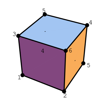
Figure 3: A three-dimensional cube $0\leq\theta_{i}\leq\frac{\pi}{2}$ ($i=1,2,3$) whose eight vertices are identified with the six Weyl group elements as shown in the picture. The 12 edges of the cube represent one parameter submanifolds of $\mathrm{SO(3)}$ where just one angle varies while the other two are at fixed values, either $0$ or $\pi/2$.

7.2 The flow diagram and the critical surfaces for $\mathrm{SL(3,\mathbb{R})}$

We can now explore the behaviour of Lax equation on the vertices, the edges and the interior of the parameter space we have described in the previous section.

Vertices

As we know from the general properties of the integral discussed in section 5 if the Lax operator lies in the Cartan subalgebra at the initial point $t=0$, namely it is diagonal it will remain constant all the time from $-\infty$ to $+\infty$. Hence on each vertex of the cube, which corresponds to a Weyl group element, we have constant Lax operators, corresponding to as many Kasner epochs.

Edges

It is interesting to see what happens on the twelve edges of the cube. Let us display the form of the matrix $\mathcal{O}$ on each of these edges.

$$\begin{array}[]{ccccc}1)&(000)&\leftrightarrow&(100)&\mathcal{O}\,=\,\left(\begin{array}[]{lll}\cos\left(\theta_{1}\right)&\sin\left(\theta_{1}\right)&0\\ -\sin\left(\theta_{1}\right)&\cos\left(\theta_{1}\right)&0\\ 0&0&1\end{array}\right)~{},\\ 2)&(000)&\leftrightarrow&(010)&\mathcal{O}\,=\,\left(\begin{array}[]{lll}1&0&0\\ 0&\cos\left(\theta_{2}\right)&\sin\left(\theta_{2}\right)\\ 0&-\sin\left(\theta_{2}\right)&\cos\left(\theta_{2}\right)\end{array}\right)~{},\\ 3)&(000)&\leftrightarrow&(001)&\mathcal{O}\,=\,\left(\begin{array}[]{lll}\cos\left(\theta_{3}\right)&0&\sin\left(\theta_{3}\right)\\ 0&1&0\\ -\sin\left(\theta_{3}\right)&0&\cos\left(\theta_{3}\right)\end{array}\right)~{},\end{array}$$ (7.53)

$$\begin{array}[]{ccccc}4)&(100)&\leftrightarrow&(110)&\mathcal{O}\,=\,\left(\begin{array}[]{lll}0&\cos\left(\theta_{2}\right)&\sin\left(\theta_{2}\right)\\ -1&0&0\\ 0&-\sin\left(\theta_{2}\right)&\cos\left(\theta_{2}\right)\end{array}\right)~{},\\ 5)&(100)&\leftrightarrow&(101)&\mathcal{O}\,=\,\left(\begin{array}[]{lll}0&1&0\\ -\cos\left(\theta_{3}\right)&0&-\sin\left(\theta_{3}\right)\\ -\sin\left(\theta_{3}\right)&0&\cos\left(\theta_{3}\right)\end{array}\right)~{},\\ 6)&(010)&\leftrightarrow&(011)&\mathcal{O}\,=\,\left(\begin{array}[]{lll}\cos\left(\theta_{3}\right)&0&\sin\left(\theta_{3}\right)\\ -\sin\left(\theta_{3}\right)&0&\cos\left(\theta_{3}\right)\\ 0&-1&0\end{array}\right)~{},\\ \end{array}$$ (7.54)

$$\begin{array}[]{ccccc}7)&(010)&\leftrightarrow&(110)&\mathcal{O}\,=\,\left(\begin{array}[]{lll}\cos\left(\theta_{1}\right)&0&\sin\left(\theta_{1}\right)\\ -\sin\left(\theta_{1}\right)&0&\cos\left(\theta_{1}\right)\\ 0&-1&0\end{array}\right)~{},\\ 8)&(001)&\leftrightarrow&(101)&\mathcal{O}\,=\,\left(\begin{array}[]{lll}0&\sin\left(\theta_{1}\right)&\cos\left(\theta_{1}\right)\\ 0&\cos\left(\theta_{1}\right)&-\sin\left(\theta_{1}\right)\\ -1&0&0\end{array}\right)~{},\\ 9)&(001)&\leftrightarrow&(011)&\mathcal{O}\,=\,\left(\begin{array}[]{lll}0&0&1\\ -\sin\left(\theta_{2}\right)&\cos\left(\theta_{2}\right)&0\\ -\cos\left(\theta_{2}\right)&-\sin\left(\theta_{2}\right)&0\end{array}\right)~{},\end{array}$$ (7.55)

$$\begin{array}[]{ccccc}10)&(110)&\leftrightarrow&(111)&\mathcal{O}\,=\,\left(\begin{array}[]{lll}-\sin\left(\theta_{3}\right)&0&\cos\left(\theta_{3}\right)\\ -\cos\left(\theta_{3}\right)&0&-\sin\left(\theta_{3}\right)\\ 0&-1&0\end{array}\right)~{},\\ 11)&(011)&\leftrightarrow&(111)&\mathcal{O}\,=\,\left(\begin{array}[]{lll}-\sin\left(\theta_{1}\right)&0&\cos\left(\theta_{1}\right)\\ -\cos\left(\theta_{1}\right)&0&-\sin\left(\theta_{1}\right)\\ 0&-1&0\end{array}\right)~{},\\ 12)&(101)&\leftrightarrow&(111)&\mathcal{O}\,=\,\left(\begin{array}[]{lll}-\sin\left(\theta_{2}\right)&\cos\left(\theta_{2}\right)&0\\ 0&0&-1\\ -\cos\left(\theta_{2}\right)&-\sin\left(\theta_{2}\right)&0\end{array}\right).\end{array}$$ (7.56)

On each link we have one of the three one-parameter subgroups respectively generated by $J_{1,2,3}$ multiplied on the left or on the right by a Weyl group element. By means of a computer programme we can then easily evaluate the general integral on each of these links. For instance on the link number $1$ we obtain:

$$L(t) = \left(\begin{array}[]{ccc}L_{11}(t)&L_{12}(t)&0\\ L_{12}(t)&L_{22}(t)&0\\ 0&0&-\lambda_{1}\,-\,\lambda_{2}\end{array}\right)~{},$$ (7.60)

$$L_{11}(t) = \frac{e^{2t\lambda_{2}}\lambda_{1}\cos^{2}\left(\theta_{1}\right)+e^{2t\lambda_{1}}\sin^{2}\left(\theta_{1}\right)\lambda_{2}}{e^{2t\lambda_{2}}\cos^{2}\left(\theta_{1}\right)+e^{2t\lambda_{1}}\sin^{2}\left(\theta_{1}\right)}~{},$$

$$L_{22}(t) = \frac{e^{2t\lambda_{2}}\lambda_{2}\cos^{2}\left(\theta_{1}\right)+e^{2t\lambda_{1}}\sin^{2}\left(\theta_{1}\right)\lambda_{1}}{e^{2t\lambda_{2}}\cos^{2}\left(\theta_{1}\right)+e^{2t\lambda_{1}}\sin^{2}\left(\theta_{1}\right)}~{},$$

$$L_{12}(t) = \frac{e^{t\left(\lambda_{1}+\lambda_{2}\right)}\sin\left(2\theta_{1}\right)\left(\lambda_{1}-\lambda_{2}\right)}{\left(-e^{2t\lambda_{1}}+e^{2t\lambda_{2}}\right)\cos\left(2\theta_{1}\right)+e^{2t\lambda_{1}}+e^{2t\lambda_{2}}}~{}.$$ (7.61)

We can also calculate the asymptotic limits of the Lax operator at $\pm\infty$ for each of these flows. As it follows from the properties of the general integral, at remotely early or at remotely late times the Lax operator is always diagonal and its eigenvalues are organized in one of the possible six ways corresponding to the six Weyl group elements acting on their reference order $(\lambda_{1},\lambda_{2},-\lambda_{1}\,-\,\lambda_{3})$. If we associate an arrow to each of these twelve links and we take into account the identification of vertices as displayed in eq.(7.48) we obtain the flow diagram shown in fig.4.

Figure 4: The oriented diagram of the $\mathrm{SL(3,\mathbb{R})}/\mathrm{SO(3)}$ flows. The Lie algebra $\mathrm{sl(3,\mathbb{R})}$ is the maximally split real section of the complex Lie algebra $\mathrm{A}_{2}$. Its Weyl group is $\mathrm{S}_{3}$ and has six elements identified by their action on the eigenvalues $\lambda_{1},\lambda_{2},\lambda_{3}$ of the Lax operator. Six are therefore the possible asymptotic states of the universe at $\pm\infty$ and each possible motion is an oriented flow from one lower Weyl element to another higher one. The lines of the graph on the right represent possible oriented flows along one-dimensional submanifolds of the parameter space located on the edges of the cube defined by restricting the range of the three Euler angles $\left\{\theta_{1},\theta_{2},\theta_{3}\right\}$ to the closed interval $\left[0,{\textstyle\frac{\pi}{2}}\right]$. On the vertices of the cube we find $\mathrm{SO(3)}$ group elements lying in the Weyl group (modulo the center $\mathbb{Z}^{3}_{2}$), just as shown in the three-dimensional picture on the right. In the two-dimensional picture on the left, by choosing as fundamental eigenvalues $\lambda_{1}=1,\lambda_{2}=2,\lambda_{3}=-3$ the Weyl group element $w_{i}\,\in\,\mathcal{W}$ is identified by the point in the plane that has coordinates equal to the projections of $w_{i}\,(\lambda_{1},\lambda_{2},\lambda_{3})$ along an orthonormal basis of vectors spanning the plane orthogonal to $(1,1,1).$

As it is clear from the quoted picture, the flows on the edges of the cube relate states of the Universe where there is no complete sorting of the eigenvalues at past and future infinities. Indeed if we use as reference set the eigenvalues of eq.(7.34) then complete sorting would require $w_{2}\,\in\,\mathcal{W}$ at $-\infty$, corresponding to the decreasing ordering $2,1,-3$ and $w_{6}$ at $+\infty$ corresponding to the increasing ordering $-3,1,2$ as we already observed. As it is evident by inspection, the matrices located on the twelve edges define one-dimensional critical surfaces. It is a a fundamental property of the Lax equation that flows touching upon a critical surface are completely constrained on it. Hence flows touching one link just lie on that link at all instants of time and the asymptotic states correspond to the vertices located at the endpoints of that link. The orientation of the link is also decided a priori. Past infinity is the lower of the two end point Weyl elements while future infinity is the higher one. This is just evident by comparing the graph in fig.(4) with the ordering of Weyl group elements as displayed in table 1.

Besides one-dimensional critical surfaces (the links) there are also two-dimensional ones (the faces) and these are obtained by studying the minors of $\mathcal{O}$.

Faces

Let us consider the orthogonal matrix $\mathcal{O}\,\in\,\mathrm{SO(3)}$ and let us name and parameterize its entries as in eq.s(LABEL:Pspec,7.40). Then there are in general exactly $6$ minors that correspond to the conditions involved in the definition of trapped surfaces in Section 5.2. Since we are dealing with $\mathfrak{sl}(3)$ all trapped surfaces are also critical. Three of the relevant minors are $1\times 1$ minors and three of them are $2\times 2$ minors. Imposing their vanishing one obtains equations on the three parameters $\theta_{1},\theta_{2},\theta_{3}$ which would define as many critical surfaces, namely six. Let us enumerate these candidate trapped and critical surfaces

$$\begin{array}[]{ccrcccl}\Sigma_{1}&:&O_{1,1}&=&0&=&\cos\left(\theta_{1}\right)\cos\left(\theta_{3}\right)-\sin\left(\theta_{1}\right)\sin\left(\theta_{2}\right)\sin\left(\theta_{3}\right)~{},\\ \Sigma_{2}&:&O_{2,1}&=&0&=&-\cos\left(\theta_{3}\right)\sin\left(\theta_{1}\right)-\cos\left(\theta_{1}\right)\sin\left(\theta_{2}\right)\sin\left(\theta_{3}\right)~{},\\ \Sigma_{3}&:&O_{3,1}&=&0&=&-\cos\left(\theta_{2}\right)\sin\left(\theta_{3}\right)~{},\\ \Sigma_{4}&:&O_{1,1}O_{2,2}-O_{1,2}O_{2,1}&=&0&=&\cos\left(\theta_{2}\right)\cos\left(\theta_{3}\right)~{},\\ \Sigma_{5}&:&O_{1,1}O_{3,2}-O_{1,2}O_{3,1}&=&0&=&\sin\left(\theta_{1}\right)\sin\left(\theta_{3}\right)-\cos\left(\theta_{1}\right)\cos\left(\theta_{3}\right)\sin\left(\theta_{2}\right)~{},\\ \Sigma_{6}&:&O_{2,1}O_{3,2}-O_{2,2}O_{3,1}&=&0&=&\cos\left(\theta_{3}\right)\sin\left(\theta_{1}\right)\sin\left(\theta_{2}\right)+\cos\left(\theta_{1}\right)\sin\left(\theta_{3}\right)~{}.\end{array}$$ (7.62)

It is now fairly simple to verify that, while the equations for $\Sigma_{1},\Sigma_{3},\Sigma_{4},$ and $\Sigma_{5}$ can be solved inside the cube $0\leq\theta_{i}\leq\frac{\pi}{2}$, all solutions of the equations for $\Sigma_{2}$ and $\Sigma_{6}$ are located outside this range. The existing inside the cube critical surfaces are shown in fig.s 5, 6, 7.

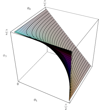
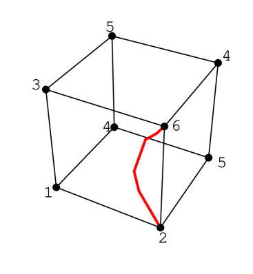
Figure 5: The picture on the left shows the critical surfaces $\Sigma_{1}$ defined by the equation $O_{1,1}=0$ imposed on the $\mathrm{SO(3)}$ group element. The picture on the right reminds the reader of the Weyl group elements located at the vertices of the parameter space. The vertices belonging the surface are (in increasing order) $w_{2},\,w_{5},\,w_{3},\,w_{6}$ so that the flow is $w_{2}\,\mapsto\,w_{6}$.

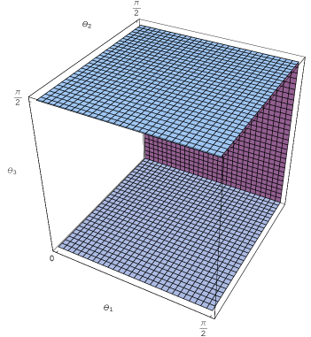
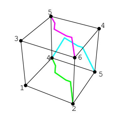
Figure 6: The picture on the left shows the union of the critical surfaces $\Sigma_{3}$ and $\Sigma_{4}$, respectively defined by the equations $O_{3,1}=0$ and $O_{1,1}O_{2,2}-O_{1,2}O_{2,1}=0$ imposed on the minors of the $\mathrm{SO(3)}$ group element. The picture on the right reminds the reader of the Weyl group elements located at the vertices of the parameter space and shows the possible oriented flows on the critical surfaces. The vertices belonging to $\Sigma_{3}$ are $w_{2},\,w_{1},\,w_{5},\,w_{4}$ and the flow on this surface is $w_{2}\,\mapsto\,w_{4}$. The vertices belonging to $\Sigma_{4}$ are instead $w_{5},\,w_{3},\,w_{4},\,w_{6}$ and the flow on this surface is $w_{5}\,\mapsto\,w_{6}$. The plaquette $\theta_{2}=\frac{\pi}{2}$ is actually the intersection $\Sigma_{3}\,\bigcap\,\Sigma_{4}$ and on this surfaces the flow goes from the lowest to the highest of the elements in the set of the vertices accessible to both surfaces, namely we have $w_{5}\,\mapsto\,w_{4}$.

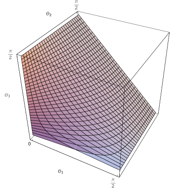
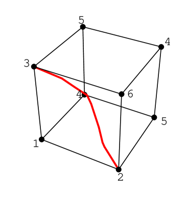
Figure 7: The picture on the left shows the critical surfaces $\Sigma_{5}$ defined by the equation $O_{1,1}O_{3,2}-O_{1,2}O_{3,1}=0$ imposed on the $\mathrm{SO(3)}$ group element. The identification of the cube vertices with Weyl group elements is shown on the right. Here the accessible vertices are $w_{2},\,w_{1},\,w_{5},\,w_{3}$ and the flow on this surface is $w_{2}\,\mapsto\,w_{3}$.

By means of a computer programme we can evaluate the flows on all these critical surfaces and we find the following results for the asymptotic values of the Lax operator:

$$\begin{array}[]{ccrcl}\Sigma_{1}&:&w_{2}&\rightarrow&w_{6}\mbox{ (surface equation $\theta_{1}=\arccos\left(\frac{\sin\left(\theta_{2}\right)\sin\left(\theta_{3}\right)}{\sqrt{\cos^{2}\left(\theta_{3}\right)+\sin^{2}\left(\theta_{2}\right)\sin^{2}\left(\theta_{3}\right)}}\right)$)}~{},\\ \Sigma_{3}&:&w_{2}&\rightarrow&w_{4}\mbox{ (for $\theta_{3}=0$)}~{},\\ \Sigma_{4}&:&w_{5}&\rightarrow&w_{6}\mbox{ (for $\theta_{3}={\textstyle\frac{\pi}{2}}$)}~{},\\ \Sigma_{3}\,\bigcap\,\Sigma_{4}&:&w_{5}&\rightarrow&w_{4}\mbox{ (for $\theta_{2}={\textstyle\frac{\pi}{2}}$)}~{},\\ \Sigma_{5}&:&w_{2}&\rightarrow&w_{3}\mbox{ (surface equation $\theta_{3}=\arccos\left(\frac{\sin\left(\theta_{1}\right)}{\sqrt{\sin^{2}\left(\theta_{1}\right)+\cos^{2}\left(\theta_{1}\right)\sin^{2}\left(\theta_{2}\right)}}\right)$)}~{}.\end{array}$$ (7.63)

The fourth case listed in eq.(7.63) needs a comment. When we set $\theta_{2}={\textstyle\frac{\pi}{2}}$ it happens that both $O_{3,1}=0$ and $O_{1,1}\,O_{2,2}\,-\,O_{1,2}\,O_{2,1}\,=\,0$. Hence this plaquette of the hypercube is actually the intersection of two critical surfaces. Altogether the result displayed in eq.(7.63) could be predicted a priori relying on the notion of accessible vertices. Given the equation of a critical surface, the accessible vertices are defined as those Weyl elements which have at least one representative satisfying the defining condition and therefore belong to the surface. Once the accessible set is defined, the flow is easily singled out. It goes from the lowest Weyl member of the set to the highest one. This task is easily carried through in the present case. For the six surfaces defined in equation (7.62) the corresponding accessible sets are rapidly calculated and we find the result displayed in table 2.

$$\begin{array}[]{|c|c|c|c|}\hline\cr\mbox{Surf.}&\mbox{Equation}&\mbox{Accessible Vertex}&\mbox{Flow}\\ \hline\cr\Sigma_{1}&O_{1,1}\,=\,0&\left(\begin{array}[]{cc}0&w_{2}\\ 1&w_{5}\\ 2&w_{3}\\ 3&w_{6}\end{array}\right)&w_{2}\,\mapsto\,w_{6}\\ \hline\cr\Sigma_{2}&O_{2,1}\,=\,0&\left(\begin{array}[]{cc}1&w_{1}\\ 2&w_{3}\\ 2&w_{4}\\ 3&w_{6}\end{array}\right)&w_{1}\,\mapsto\,w_{6}\\ \hline\cr\Sigma_{3}&O_{3,1}\,=\,0&\left(\begin{array}[]{cc}0&w_{2}\\ 1&w_{1}\\ 1&w_{5}\\ 2&w_{4}\end{array}\right)&w_{2}\,\mapsto\,w_{4}\\ \hline\cr\Sigma_{4}&-O_{1,2}\,O_{2,1}\,+\,O_{1,1}\,O_{2,2}\,=\,0&\left(\begin{array}[]{cc}1&w_{5}\\ 2&w_{3}\\ 2&w_{4}\\ 3&w_{6}\end{array}\right)&w_{5}\,\mapsto\,w_{6}\\ \hline\cr\Sigma_{5}&-O_{1,2}\,O_{3,1}\,+\,O_{1,1}\,O_{3,2}\,=\,0&\left(\begin{array}[]{cc}0&w_{2}\\ 1&w_{1}\\ 1&w_{5}\\ 2&w_{3}\end{array}\right)&w_{2}\,\mapsto\,w_{3}\\ \hline\cr\Sigma_{6}&-O_{2,2}\,O_{3,1}\,+\,O_{2,1}\,O_{3,2}\,=\,0&\left(\begin{array}[]{cc}0&w_{2}\\ 1&w_{1}\\ 2&w_{4}\\ 3&w_{6}\end{array}\right)&w_{2}\,\mapsto\,w_{6}\\ \hline\cr\end{array}$$

Table 2: The accessible vertices for each of the six two-dimensional critical surfaces in the case $\mathrm{SL(3,\mathbb{R})/\mathrm{SO(3)}}$.

Expunging surfaces $\Sigma_{2}$ and $\Sigma_{6}$ which fall outside the cube, we find that the available flows on critical two dimensional surfaces inside the cube are just only four, namely the following ones:

$$w_{2}\,\mapsto\,w_{6}~{},$$

$$w_{2}\,\mapsto\,w_{4}~{},$$

$$w_{5}\,\mapsto\,w_{6}~{},$$

$$w_{2}\,\mapsto\,w_{3}~{}.$$ (7.64)

The only non vanishing intersection of these surfaces is the afore-mentioned plaquette $\Sigma_{3}\,\bigcap\,\Sigma_{4}$. We can easily calculate the intersection of vertices accessible to both $\Sigma_{3}$ and $\Sigma_{4}$. We find

$$\left\{w_{2},w_{1},w_{5},w_{4}\right\}\,\bigcap\,\left\{w_{5},w_{3},w_{4},w_{6}\right\}\,=\,\left\{w_{5},w_{4}\right\}$$ (7.65)

where all sets are written in ascending order. It follows that on the surface $\Sigma_{3}\,\bigcap\,\Sigma_{4}$ the oriented flow is

$$w_{5}\,\mapsto\,w_{4}$$ (7.66)

as indeed it is verified by numerical calculation on the computer.

This concludes our discussion of the $\mathrm{SL(3,\mathbb{R})}$ which has been instrumental to illustrate the involved mathematical structures.

We have seen that the topology of the parameter space $\mathrm{H}/\mathcal{W}(\mathbb{U})$ is indeed complicated and cannot be easily displayed as an hypercube. Yet it is completely defined by the trapped hypersurfaces which admit a clear definition in terms of algebraic equations. These surfaces split the parameter space $\mathrm{H}/\mathcal{W}(\mathbb{U})$ into convex hulls which are separated from each other. Indeed the walls are impenetrable according to Toda evolution. Moreover we can relate the initial and final states of the flows to these critical surfaces defined by the vanishing of the relevant minors in the orthogonal matrix $\mathcal{O}$.

Our next section is devoted to another maximal split case of rank $r=2$ which will correspond to an entire Tits Satake universality class of cases.

8 The maximally split case $\mathrm{Sp(4,\mathbb{R})}/\mathrm{U(2)}$

As we explained in the introduction our goal is the illustration of the Lax integration formula in the non-maximally split case $\mathrm{SO(r,r+2s)}/\mathrm{SO(r)}\times\mathrm{SO(r+2s)}$. The Tits Satake projection of these manifolds is provided by the maximally split coset

$$\mathcal{M}^{TS}_{r}\,\equiv\,\frac{\mathrm{SO(r,r+1)}}{\mathrm{SO(r)}\times\mathrm{SO(r+1)}}~{}.$$ (8.1)

In the case of rank $r=2$ we have

$$\mathcal{M}^{TS}_{2}\,\equiv\,\frac{\mathrm{SO(2,3)}}{\mathrm{SO(2)}\times\mathrm{SO(3)}}\,=\,\frac{\mathrm{Sp(4,\mathbb{R})}}{\mathrm{U(2)}}$$ (8.2)

due to the accidental isomorphism between the $B_{2}$ and $C_{2}$ Lie algebras whose Dynkin diagram is displayed in fig. 8.

Figure 8: The Dynkin diagram of the $B_{2}\sim C_{2}$ Lie algebra.

For this reason we can rely on either formulation in terms of $4\times 4$ symplectic matrices or $5\times 5$ pseudo-orthogonal matrices to obtain the same result.

In the symplectic $\mathfrak{sp}(4)$ interpretation, the $C_{2}$ root system can be realized by the following eight two-dimensional vectors:

$$\Delta_{C_{2}}=\left\{\pm\epsilon^{i}\,\pm\,\epsilon^{j}\,,\,\pm\epsilon^{i}\right\}$$ (8.3)

where $\epsilon^{i}\,(i=1,2)$ denotes a basis of orthonormal unit vectors. In the pseudo-orthogonal $\mathfrak{so}(2,3)$ interpretation of the same algebra the $B_{2}$ root system is instead realized by the following eight vectors:

$$\Delta_{B_{2}}=\left\{\pm\epsilon^{i}\,\pm\,\epsilon^{j}\,,\,\pm 2\,\epsilon^{i}\right\}~{}.$$ (8.4)

The two root systems are displayed in fig. 9.

Figure 9: The $C_{2}$ and $B_{2}$ root systems. They are related by the exchange of the long with the short roots and viceversa.

8.1 The Weyl group and the generalized Weyl group of $\mathfrak{sp}(4,\mathbb{R})$

Abstractly the Weyl group $\mathrm{Weyl}(C_{2})$ of the Lie algebra $\mathfrak{sp}(4,\mathbb{R})$ is given by $(\mathbb{Z}_{2}\times\mathbb{Z}_{2})\,\ltimes\,\mathrm{S}_{2}$ and its eight elements $w_{i}\in\mathrm{Weyl}(C_{2})$ can be described by their action on the two Cartan fields $h_{1},h_{2}$

$$\begin{array}[]{ccccl}w_{1}&:&(h_{1},h_{2})&\rightarrow&(h_{1},h_{2})~{},\\ w_{2}&:&(h_{1},h_{2})&\rightarrow&(-h_{1},-h_{2})~{},\\ w_{3}&:&(h_{1},h_{2})&\rightarrow&(-h_{1},h_{2})~{},\\ w_{4}&:&(h_{1},h_{2})&\rightarrow&(h_{1},-h_{2})~{},\\ w_{5}&:&(h_{1},h_{2})&\rightarrow&(h_{2},h_{1})~{},\\ w_{6}&:&(h_{1},h_{2})&\rightarrow&(h_{2},-h_{1})~{},\\ w_{7}&:&(h_{1},h_{2})&\rightarrow&(-h_{2},h_{1})~{},\\ w_{8}&:&(h_{1},h_{2})&\rightarrow&(-h_{2},-h_{1})~{}.\\ \end{array}$$ (8.5)

Just as we did in the previous case study we can introduce a partial ordering of the Weyl group elements which will govern the orientation of all dynamical flows. The key point is the embedding

$$\mathrm{Weyl}\left(\mathfrak{sp}(4)\right)\,\hookrightarrow\,\mathcal{S}_{4}\,\simeq\,\mathrm{Weyl}\left(\mathfrak{sl}(4)\right)$$ (8.6)

of the Weyl group into the symmetric group $\mathcal{S}_{4}$ induced by the $4\times 4$ representation of the Lie algebra $\mathfrak{sp}(4)$ in which the solvable Lie algebra is made of upper triangular matrices. The explicit construction of such a representation is performed in the next section. For the purpose of the considered issue, namely discovering the structure of the generalized Weyl group and ordering of Weyl group elements, we anticipate some results. The matrices corresponding to Cartan subalgebra elements are of the following form:

$$\mbox{CSA}\,\ni\,\left(\begin{array}[]{cccc}h_{1}&0&0&0\\ 0&h_{2}&0&0\\ 0&0&-h_{2}&0\\ 0&0&0&-h_{1}\end{array}\right)~{}.$$ (8.7)

In this way, the action of each Weyl group element as defined in eq.(8.5) can be reinterpreted as a particular permutation of the set $\left(h_{1},h_{2},-h_{2},-h_{1}\right)$ and this interpretation provides the embedding (8.6). To make it precise let us derive the structure of the generalized Weyl group. Following the definition 5.1 we introduce as generators the operator defined in eq.(8.33) for the following four choices of the $\theta$-angles:

$$\left\{\theta_{1}\,,\,\theta_{2}\,,\,\theta_{3}\,,\,\theta_{4}\right\}\,=\,\left\{\begin{array}[]{cccc}\frac{\pi}{2}&0&0&0\\ 0&\frac{\pi}{2}&0&0\\ 0&0&\frac{\pi}{2}&0\\ 0&0&0&\frac{\pi}{2}\end{array}\right.$$ (8.8)

which just corresponds to the $4$ roots of $\mathfrak{sp}(4)$. By closing the shell of products we obtain a group with $32$-elements, $\mathcal{W}(\mathfrak{sp}(4))$. This group has an order four normal subgroup $\mathrm{N}(\mathfrak{sp}(4))$ with the structure of $\mathbb{Z}_{2}\,\times\,\mathbb{Z}_{2}$ whose adjoint action on any of the Cartan matrices (8.7) is the identity. Explicitly $\mathrm{N}(\mathfrak{sp}(4))$ is made by the following four symplectic matrices:

$$\begin{array}[]{rclcrcl}N_{1}&=&\left(\begin{array}[]{llll}-1&0&0&0\\ 0&-1&0&0\\ 0&0&-1&0\\ 0&0&0&-1\end{array}\right)&;&N_{2}&\simeq&\left(\begin{array}[]{llll}-1&0&0&0\\ 0&1&0&0\\ 0&0&1&0\\ 0&0&0&-1\end{array}\right)~{},\end{array}$$ (8.9)

$$\begin{array}[]{rclcrcl}N_{3}&\simeq&\left(\begin{array}[]{llll}1&0&0&0\\ 0&-1&0&0\\ 0&0&-1&0\\ 0&0&0&1\end{array}\right)&;&N_{4}&\simeq&\left(\begin{array}[]{llll}1&0&0&0\\ 0&1&0&0\\ 0&0&1&0\\ 0&0&0&1\end{array}\right)~{}.\\ \end{array}$$ (8.10)

As expected the factor group $\mathcal{W}(\mathfrak{sp}(4))/\mathrm{N}(\mathfrak{sp}(4))$ is isomorphic to the Weyl group $\mathrm{Weyl}\left(\mathfrak{sp}(4)\right)$ since the adjoint action of each equivalence class produces the same transformation on the eigenvalues $h_{1},h_{2}$ as the abstract Weyl elements listed in eq.(8.5). Explicitly the $8$-equivalence classes of $4$-elements each are displayed below

$$\begin{array}[]{rclcrcl}\Omega_{1}&\simeq&\left(\begin{array}[]{llll}1&0&0&0\\ 0&1&0&0\\ 0&0&1&0\\ 0&0&0&1\end{array}\right)\,\mathrm{N}(\mathfrak{sp}(4))&;&\Omega_{2}&\simeq&\left(\begin{array}[]{llll}0&0&0&1\\ 0&0&1&0\\ 0&-1&0&0\\ -1&0&0&0\end{array}\right)\,\mathrm{N}(\mathfrak{sp}(4))~{},\end{array}$$ (8.11)

$$\begin{array}[]{rclcrcl}\Omega_{3}&\simeq&\left(\begin{array}[]{llll}0&0&0&1\\ 0&1&0&0\\ 0&0&1&0\\ -1&0&0&0\end{array}\right)\,\mathrm{N}(\mathfrak{sp}(4))&;&\Omega_{4}&\simeq&\left(\begin{array}[]{llll}1&0&0&0\\ 0&0&1&0\\ 0&-1&0&0\\ 0&0&0&1\end{array}\right)\,\mathrm{N}(\mathfrak{sp}(4))\\ \end{array}~{},$$ (8.12)

$$\begin{array}[]{rclcrcl}\Omega_{5}&\simeq&\left(\begin{array}[]{llll}0&1&0&0\\ 1&0&0&0\\ 0&0&0&1\\ 0&0&1&0\end{array}\right)\,\mathrm{N}(\mathfrak{sp}(4))&;&\Omega_{6}&\simeq&\left(\begin{array}[]{llll}0&0&1&0\\ 1&0&0&0\\ 0&0&0&1\\ 0&-1&0&0\end{array}\right)\,\mathrm{N}(\mathfrak{sp}(4))~{},\\ \end{array}$$ (8.13)

$$\begin{array}[]{rclcrcl}\Omega_{7}&\simeq&\left(\begin{array}[]{llll}0&1&0&0\\ 0&0&0&1\\ -1&0&0&0\\ 0&0&1&0\end{array}\right)\,\mathrm{N}(\mathfrak{sp}(4))&;&\Omega_{8}&\simeq&\left(\begin{array}[]{llll}0&0&1&0\\ 0&0&0&1\\ -1&0&0&0\\ 0&-1&0&0\end{array}\right)\,\mathrm{N}(\mathfrak{sp}(4))~{}.\end{array}$$ (8.14)

Considering now a Cartan Lie algebra element in the fundamental representation of $\mathfrak{sp}(4,\mathbb{R})$ as given in eq.(8.7) we have

$$\forall w_{i}\,\in\,Weyl(C_{2})\quad:\quad\Omega_{i}^{T}\,\mathcal{C}\left(\{h_{1},h_{2}\}\right)\,\Omega_{i}\,=\,\mathcal{C}\left(w_{i}\{h_{1},h_{2}\}\right)~{}.$$ (8.15)

This being established let us choose as conventional reference set of eigenvalues the following one:

$$h_{1}\,=\,1\quad;\quad h_{2}\,=\,2~{},$$ (8.16)

then the decreasing sorting to be expected at past infinity is $2,1,-1,-2$ and corresponds to the Weyl element $\Omega_{5}$. If we take this as the fundamental permutation, all the other eight permutations belonging to the Weyl group can be ranked with the number of transpositions needed to bring them to the fundamental one. This procedure provides the partial ordering of the Weyl group displayed in table 3.

$$\begin{array}[]{|c|c|}\hline\cr\ell_{T}&\mbox{Weyl group}\\ \hbox{}\hfil&\mbox{of $\mathfrak{sp}(4,\mathbb{R})$}\\ \hline\cr 0&w_{5}\\ 1&w_{6}\\ 2&w_{1}\\ 3&w_{3}\\ 3&w_{4}\\ 4&w_{2}\\ 5&w_{7}\\ 6&w_{8}\\ \hline\cr\end{array}$$

Table 3: Partial ordering of the Weyl group of $\mathfrak{sp}(4,\mathbb{R}).$

We can now study the general features of the flows associated with the maximally split coset manifold (8.2) and see how they follow the general principles and connect past and future Kasner epochs ordered according to table 3. To realize this study the first essential step is the construction of the $\mathfrak{sp}(4,\mathbb{R})$ Lie algebra in a basis which fulfils the condition that the solvable Lie algebra generating the coset is represented by upper triangular matrices. The form of the Cartan subalgebra in such a basis was already anticipated in eq.(8.7), the full construction is presented in the next section.

8.2 Construction of the $\mathfrak{sp}(4,\mathbb{R})$ Lie algebra

The most compact way of presenting our basis is the following. Let us begin with the solvable Lie algebra $Solv(\mathrm{Sp(4,\mathbb{R})}/\mathrm{U(2)})$. Abstractly the most general element of this algebra is given by

$$\mathcal{T}\,=\,h_{1}\,\mathcal{H}_{1}\,+\,h_{2}\,\mathcal{H}_{2}\,+\,e_{1}\,E^{\alpha_{1}}\,+\,e_{2}\,E^{\alpha_{2}}\,+\,e_{3}\,E^{\alpha_{1}+\alpha_{2}}\,+\,e_{4}\,E^{2\alpha_{1}+\alpha_{2}}~{}.$$ (8.17)

If we write the explicit form of $\mathcal{T}$ as a $4\times 4$, upper triangular symplectic matrix

$$\mathcal{T}_{sym} = \left(\begin{array}[]{llll}h_{1}&e_{1}&e_{3}&-\sqrt{2}e_{4}\\ 0&h_{2}&\sqrt{2}e_{2}&e_{3}\\ 0&0&-h_{2}&-e_{1}\\ 0&0&0&-h_{1}\end{array}\right)\,\in\,\mathfrak{sp}(4,\mathbb{R})$$ (8.22)

which satisfies the condition

$$\mathcal{T}_{sym}^{T}\,\left(\begin{array}[]{cc}\mathbf{0}_{2}&\mathbf{1}_{2}\\ -\mathbf{1}_{2}&\mathbf{0}_{2}\end{array}\right)\,+\,\left(\begin{array}[]{cc}\mathbf{0}_{2}&\mathbf{1}_{2}\\ -\mathbf{1}_{2}&\mathbf{0}_{2}\end{array}\right)\,\mathcal{T}_{sym}\,=\,0$$ (8.23)

all the generators of the solvable algebra are defined in the four dimensional symplectic representation.

By writing the same Lie algebra element (8.17) as a $5\times 5$ matrix

$$\mathcal{T}_{so} = \left(\begin{array}[]{lllll}h_{1}+h_{2}&-\sqrt{2}e_{2}&-\sqrt{2}e_{3}&-\sqrt{2}e_{4}&0\\ 0&h_{1}-h_{2}&-\sqrt{2}e_{1}&0&\sqrt{2}e_{4}\\ 0&0&0&\sqrt{2}e_{1}&\sqrt{2}e_{3}\\ 0&0&0&h_{2}-h_{1}&\sqrt{2}e_{2}\\ 0&0&0&0&-h_{1}-h_{2}\end{array}\right)\,\in\,\mathfrak{so}(2,3)$$ (8.29)

which satisfies the condition

$$\mathcal{T}_{so}^{T}\,\left(\begin{array}[]{cc|c|cc}0&0&0&0&1\\ 0&0&0&1&0\\ \hline\cr 0&0&1&0&0\\ \hline\cr 0&1&0&0&0\\ 1&0&0&0&0\end{array}\right)\,+\,\left(\begin{array}[]{cc|c|cc}0&0&0&0&1\\ 0&0&0&1&0\\ \hline\cr 0&0&1&0&0\\ \hline\cr 0&1&0&0&0\\ 1&0&0&0&0\end{array}\right)\,\mathcal{T}_{so}\,=\,0$$ (8.30)

we define the same generators also in the five dimensional pseudo-orthogonal representation. The choice of the invariant metric displayed in eq.(8.30) is that which guarantees the upper triangular structure of the solvable Lie algebra generators. We shall come back on this point in later sections.

Once the generators of the solvable Lie algebra are given the full Lie algebra can be completed by defining the orthonormal generators of the $\mathbb{K}$ subspace as follows:

$$\mathrm{K}_{1} = \mathcal{H}_{1}~{},$$

$$\mathrm{K}_{2} = \mathcal{H}_{2}~{},$$

$$\mathrm{K}_{3} = {\textstyle\frac{1}{\sqrt{2}}}\left(E^{\alpha_{1}}\,+\,(E^{\alpha_{1}})^{T}\right)~{},$$

$$\mathrm{K}_{4} = {\textstyle\frac{1}{\sqrt{2}}}\left(E^{\alpha_{2}}\,+\,(E^{\alpha_{2}})^{T}\right)~{},$$

$$\mathrm{K}_{5} = {\textstyle\frac{1}{\sqrt{2}}}\left(E^{\alpha_{1}+\alpha_{2}}\,+\,(E^{\alpha_{1}+\alpha_{2}})^{T}\right)~{},$$

$$\mathrm{K}_{6} = {\textstyle\frac{1}{\sqrt{2}}}\left(E^{\alpha_{1}+2\alpha_{2}}\,+\,(E^{\alpha_{1}+2\alpha_{2}})^{T}\right),$$ (8.31)

and those of the maximal compact subalgebra $\mathbb{H}=\mathfrak{u}(2)$ as follows:

$$\mathrm{J}_{1} = {\textstyle\frac{1}{\sqrt{2}}}\left(E^{\alpha_{1}}\,-\,(E^{\alpha_{1}})^{T}\right)~{},$$

$$\mathrm{J}_{2} = {\textstyle\frac{1}{\sqrt{2}}}\left(E^{\alpha_{2}}\,-\,(E^{\alpha_{2}})^{T}\right)~{},$$

$$\mathrm{J}_{3} = {\textstyle\frac{1}{\sqrt{2}}}\left(E^{\alpha_{1}+\alpha_{2}}\,-\,(E^{\alpha_{1}+\alpha_{2}})^{T}\right)~{},$$

$$\mathrm{J}_{4} = {\textstyle\frac{1}{\sqrt{2}}}\left(E^{\alpha_{1}+2\alpha_{2}}\,-\,(E^{\alpha_{1}+2\alpha_{2}})^{T}\right)~{}.$$ (8.32)

In this way we have constructed all the relevant generators in both representations. The flows are clearly an intrinsic property of the algebra and will not depend on the representation chosen.

8.3 Parameterization of the compact group $\mathrm{U(2)}$ and critical submanifolds

In a way completely analogous to the previous case-study we can now parameterize the compact subgroup by writing

$$\mathcal{O}\,=\,\exp\left[\sqrt{2}\,\theta_{1}\,\mathrm{J_{1}}\right]\,\exp\left[\theta_{2}\,\mathrm{J_{2}}\right]\,\exp\left[\sqrt{2}\,\theta_{3}\,\mathrm{J_{3}}\right]\,\exp\left[\theta_{4}\,\mathrm{J_{4}}\right]~{}.$$ (8.33)

The square root of two factors have been introduced in equation (8.33) in such a way as to normalize the theta angles so that the group element $\mathcal{O}$ becomes an integer valued matrix at $\theta_{i}=\frac{\pi}{2}$. Obviously we have two instances of $\mathcal{O}$: the $4\times 4$ symplectic $\mathcal{O}_{sp}$ and the $5\times 5$ pseudo-orthogonal $\mathcal{O}_{so}$. Both of them become integer valued for the same choice of the angles and when acting by similarity transformation on the Cartan subalgebra they correspond to Weyl group elements.

For simplicity we use the $4\times 4$ representation and we find

$$\mathcal{O}\,=\,\left(\begin{array}[]{cccc}O_{11}&O_{12}&O_{13}&O_{14}\\ O_{21}&O_{22}&O_{23}&O_{24}\\ O_{31}&O_{32}&O_{33}&O_{34}\\ O_{41}&O_{42}&O_{43}&O_{44}\end{array}\right)$$ (8.34)

where

$$\begin{array}[]{ccl}O_{11}&=&\cos\theta_{1}\cos\theta_{3}\cos\theta_{4}-\sin\theta_{1}\sin\theta_{3}\sin\left(\theta_{2}-\theta_{4}\right)~{},\\ O_{12}&=&\cos\theta_{2}\cos\theta_{3}\sin\theta_{1}~{},\\ O_{13}&=&\cos\theta_{3}\sin\theta_{1}\sin\theta_{2}+\cos\theta_{1}\sin\theta_{3}~{},\\ O_{14}&=&\cos\theta_{2}\cos\theta_{4}\sin\theta_{1}\sin\theta_{3}+\left(\sin\theta_{1}\sin\theta_{2}\sin\theta_{3}-\cos\theta_{1}\cos\theta_{3}\right)\sin\theta_{4}~{},\\ \end{array}$$ (8.35)

$$\begin{array}[]{ccl}O_{21}&=&-\cos\theta_{3}\cos\theta_{4}\sin\theta_{1}-\cos\theta_{1}\sin\theta_{3}\sin\left(\theta_{2}-\theta_{4}\right)~{},\\ O_{22}&=&\cos\theta_{1}\cos\theta_{2}\cos\theta_{3}~{},\\ O_{23}&=&\cos\theta_{1}\cos\theta_{3}\sin\theta_{2}-\sin\theta_{1}\sin\theta_{3}~{},\\ O_{24}&=&\cos\theta_{1}\cos\theta_{2}-\theta_{4}\sin\theta_{3}+\cos\theta_{3}\sin\theta_{1}\sin\theta_{4}~{},\\ \end{array}$$ (8.36)

$$\begin{array}[]{ccl}O_{31}&=&-\cos\theta_{1}\cos\theta_{2}-\theta_{4}\sin\theta_{3}-\cos\theta_{3}\sin\theta_{1}\sin\theta_{4}~{},\\ O_{32}&=&\sin\theta_{1}\sin\theta_{3}-\cos\theta_{1}\cos\theta_{3}\sin\theta_{2}~{},\\ O_{32}&=&\cos\theta_{1}\cos\theta_{2}\cos\theta_{3}~{},\\ O_{33}&=&\cos\theta_{1}\cos\theta_{2}\cos\theta_{3}~{},\\ O_{34}&=&-\cos\theta_{3}\cos\theta_{4}\sin\theta_{1}-\cos\theta_{1}\sin\theta_{3}\sin\left(\theta_{2}-\theta_{4}\right)~{},\\ \end{array}$$ (8.37)

$$\begin{array}[]{ccl}O_{41}&=&\left(\cos\theta_{1}\cos\theta_{3}-\sin\theta_{1}\sin\theta_{2}\sin\theta_{3}\right)\sin\theta_{4}-\cos\theta_{2}\cos\theta_{4}\sin\theta_{1}\sin\theta_{3}~{},\\ O_{42}&=&-\cos\theta_{3}\sin\theta_{1}\sin\theta_{2}-\cos\theta_{1}\sin\theta_{3}~{},\\ O_{43}&=&\cos\theta_{2}\cos\theta_{3}\sin\theta_{1}~{},\\ O_{44}&=&\cos\theta_{1}\cos\theta_{3}\cos\theta_{4}-\sin\theta_{1}\sin\theta_{3}\sin\left(\theta_{2}-\theta_{4}\right)~{}.\end{array}$$ (8.38)

Vertices

Having parameterized in this way the $\mathrm{U(2)}$ group element with the four Euler angles $\theta_{i}$, in a completely analogous way to the case of $\mathrm{SL(3,\mathbb{R})}$, we can check that when all of the $\theta_{i}$ take either the $0$ or the $\frac{\pi}{2}$ value then the corresponding matrix $\mathcal{O}$ becomes integer valued and its similarity action on a Cartan subalgebra element (8.7) corresponds to the action of some Weyl group element on the eigenvalues:

$$\mbox{If }\forall i\,\,\theta_{i}\,=\,\left\{\begin{array}[]{c}0\\ \mathrm{or}\\ \frac{\pi}{2}\end{array}\right.\quad,\quad\exists\,\omega\,\in\,Weyl(C_{2})\quad/\quad\mathcal{O}^{T}\,\mathcal{C}\left(\{h_{1},h_{2}\}\right)\,\mathcal{O}\,=\,\mathcal{C}\left(\omega\{h_{1},h_{2}\}\right)~{}.$$ (8.39)

In this way the parameter space $\mathrm{U(2)}/\mathrm{{\cal W}}$ is reduced to lie in a four dimensional hypercube and, using a notation analogous to that of eq.(7.41), the identification of the $16$ vertices of the hypercube with Weyl group elements is displayed in table 4. As the reader can observe, in the chosen numbering the odd-labeled Weyl group elements appear only once, while the even-labeled appear three-times.

$$\begin{array}[]{|c|c|c|c|}\hline\cr\#&\mbox{vertex}&\mbox{Weyl group element}&\mbox{multiplicity of Weyl elem.}\\ \hline\cr 1&\{0,0,0,0\}&\Omega_{1}&1\\ 2&\{1,0,0,0\}&\Omega_{5}&1\\ 3&\{0,1,0,0\}&\Omega_{4}&3\\ 4&\{0,0,1,0\}&\Omega_{8}&3\\ 5&\{0,0,0,1\}&\Omega_{3}&1\\ 6&\{1,1,0,0\}&\Omega_{6}&3\\ 7&\{1,0,1,0\}&\Omega_{2}&3\\ 8&\{1,0,0,1\}&\Omega_{7}&1\\ 9&\{0,1,1,0\}&\Omega_{6}&3\\ 10&\{0,1,0,1\}&\Omega_{2}&3\\ 11&\{0,0,1,1\}&\Omega_{6}&3\\ 12&\{1,1,1,0\}&\Omega_{4}&3\\ 13&\{1,1,0,1\}&\Omega_{8}&3\\ 14&\{1,0,1,1\}&\Omega_{4}&3\\ 15&\{0,1,1,1\}&\Omega_{8}&3\\ 16&\{1,1,1,1\}&\Omega_{2}&3\\ \hline\cr\end{array}$$

Table 4: The 16 vertices of the hypercubic parameter space for $\mathrm{Sp(4,\mathbb{R})/U(2)}$ and their identification with Weyl group elements.

Edges

Using just the same strategy as in the previous case-study we can now construct the $64$ oriented links connecting the $16$ vertices. These are all the possible segments of straight lines in parameter space connecting two vertices and by means of a computer programme we can evaluate the orientation of the link, namely discover which of the end-points (Weyl group element) corresponds to past infinity $t=-\infty$ and which to future infinity $t=+\infty$. As expected the orientation of all the links is in the direction from lower to higher Weyl elements, according to the ordering of table 3. The result of these computations is displayed in table 5 and summarized in the flow diagram of fig.10.

$$\begin{array}[]{|c|ccc||c|cccc|}\hline\cr\#&\mbox{Vertex}&\mbox{Vertex}&\mbox{Flow}&\#&\mbox{Vertex}&\mbox{Vertex}&\mbox{Flow}&\\ \hline\cr 1&\{0,0,0,0\}&\{0,0,0,1\}&\mbox{$\Omega_{1}$ $\mapsto$ $\Omega_{3}$}&\hbox{}\hfil&\hbox{}\hfil&\hbox{}\hfil&\hbox{}\hfil&\hbox{}\hfil\\ 2&\{0,0,0,0\}&\{0,0,1,0\}&\mbox{$\Omega_{1}$ $\mapsto$ $\Omega_{8}$}&3&\{0,0,0,0\}&\{0,1,0,0\}&\mbox{$\Omega_{1}$ $\mapsto$ $\Omega_{4}$}&\\ 4&\ \{0,0,0,0\}&\{1,0,0,0\}&\mbox{$\Omega_{5}$ $\mapsto$ $\Omega_{1}$}&5&\{0,0,0,1\}&\{0,0,0,0\}&\mbox{$\Omega_{1}$ $\mapsto$ $\Omega_{3}$}&\\ 6&\ \{0,0,0,1\}&\{0,0,1,1\}&\mbox{$\Omega_{6}$ $\mapsto$ $\Omega_{3}$}&7&\{0,0,0,1\}&\{0,1,0,1\}&\mbox{$\Omega_{3}$ $\mapsto$ $\Omega_{2}$}&\\ 8&\ \{0,0,0,1\}&\{1,0,0,1\}&\mbox{$\Omega_{3}$ $\mapsto$ $\Omega_{7}$}&9&\{0,0,1,0\}&\{0,0,0,0\}&\mbox{$\Omega_{1}$ $\mapsto$ $\Omega_{8}$}&\\ 10&\ \{0,0,1,0\}&\{0,0,1,1\}&\mbox{$\Omega_{6}$ $\mapsto$ $\Omega_{8}$}&11&\{0,0,1,0\}&\{0,1,1,0\}&\mbox{$\Omega_{6}$ $\mapsto$ $\Omega_{8}$}&\\ 12&\ \{0,0,1,0\}&\{1,0,1,0\}&\mbox{$\Omega_{2}$ $\mapsto$ $\Omega_{8}$}&13&\{0,0,1,1\}&\{0,0,0,1\}&\mbox{$\Omega_{6}$ $\mapsto$ $\Omega_{3}$}&\\ 14&\ \{0,0,1,1\}&\{0,0,1,0\}&\mbox{$\Omega_{6}$ $\mapsto$ $\Omega_{8}$}&15&\{0,0,1,1\}&\{0,1,1,1\}&\mbox{$\Omega_{6}$ $\mapsto$ $\Omega_{8}$}&\\ 16&\ \{0,0,1,1\}&\{1,0,1,1\}&\mbox{$\Omega_{6}$ $\mapsto$ $\Omega_{4}$}&17&\{0,1,0,0\}&\{0,0,0,0\}&\mbox{$\Omega_{1}$ $\mapsto$ $\Omega_{4}$}&\\ 18&\ \{0,1,0,0\}&\{0,1,0,1\}&\mbox{$\Omega_{4}$ $\mapsto$ $\Omega_{2}$}&19&\{0,1,0,0\}&\{0,1,1,0\}&\mbox{$\Omega_{6}$ $\mapsto$ $\Omega_{4}$}&\\ 20&\ \{0,1,0,0\}&\{1,1,0,0\}&\mbox{$\Omega_{6}$ $\mapsto$ $\Omega_{4}$}&21&\{0,1,0,1\}&\{0,0,0,1\}&\mbox{$\Omega_{3}$ $\mapsto$ $\Omega_{2}$}&\\ 22&\ \{0,1,0,1\}&\{0,1,0,0\}&\mbox{$\Omega_{4}$ $\mapsto$ $\Omega_{2}$}&23&\{0,1,0,1\}&\{0,1,1,1\}&\mbox{$\Omega_{2}$ $\mapsto$ $\Omega_{8}$}&\\ 24&\ \{0,1,0,1\}&\{1,1,0,1\}&\mbox{$\Omega_{2}$ $\mapsto$ $\Omega_{8}$}&25&\{0,1,1,0\}&\{0,0,1,0\}&\mbox{$\Omega_{6}$ $\mapsto$ $\Omega_{8}$}&\\ 26&\ \{0,1,1,0\}&\{0,1,0,0\}&\mbox{$\Omega_{6}$ $\mapsto$ $\Omega_{4}$}&27&\{0,1,1,0\}&\{0,1,1,1\}&\mbox{$\Omega_{6}$ $\mapsto$ $\Omega_{8}$}&\\ 28&\ \{0,1,1,0\}&\{1,1,1,0\}&\mbox{$\Omega_{6}$ $\mapsto$ $\Omega_{4}$}&29&\{0,1,1,1\}&\{0,0,1,1\}&\mbox{$\Omega_{6}$ $\mapsto$ $\Omega_{8}$}&\\ 30&\ \{0,1,1,1\}&\{0,1,0,1\}&\mbox{$\Omega_{2}$] $\mapsto$ $\Omega_{8}$}&31&\{0,1,1,1\}&\{0,1,1,0\}&\mbox{$\Omega_{6}$ $\mapsto$ $\Omega_{8}$}&\\ 32&\ \{0,1,1,1\}&\{1,1,1,1\}&\mbox{$\Omega_{2}$ $\mapsto$ $\Omega_{8}$}&33&\{1,0,0,0\}&\{0,0,0,0\}&\mbox{$\Omega_{5}$ $\mapsto$ $\Omega_{1}$}&\\ 34&\ \{1,0,0,0\}&\{1,0,0,1\}&\mbox{$\Omega_{5}$ $\mapsto$ $\Omega_{7}$}&35&\{1,0,0,0\}&\{1,0,1,0\}&\mbox{$\Omega_{5}$ $\mapsto$ $\Omega_{2}$}&\\ 36&\ \{1,0,0,0\}&\{1,1,0,0\}&\mbox{$\Omega_{5}$ $\mapsto$ $\Omega_{6}$}&37&\{1,0,0,1\}&\{0,0,0,1\}&\mbox{$\Omega_{3}$ $\mapsto$ $\Omega_{7}$}&\\ 38&\ \{1,0,0,1\}&\{1,0,0,0\}&\mbox{$\Omega_{5}$ $\mapsto$ $\Omega_{7}$}&39&\{1,0,0,1\}&\{1,0,1,1\}&\mbox{$\Omega_{4}$ $\mapsto$ $\Omega_{7}$}&\\ 40&\ \{1,0,0,1\}&\{1,1,0,1\}&\mbox{$\Omega_{7}$ $\mapsto$ $\Omega_{8}$}&41&\{1,0,1,0\}&\{0,0,1,0\}&\mbox{$\Omega_{2}$ $\mapsto$ $\Omega_{8}$}&\\ 42&\ \{1,0,1,0\}&\{1,0,0,0\}&\mbox{$\Omega_{5}$ $\mapsto$ $\Omega_{2}$}&43&\{1,0,1,0\}&\{1,0,1,1\}&\mbox{$\Omega_{4}$ $\mapsto$ $\Omega_{2}$}&\\ 44&\ \{1,0,1,0\}&\{1,1,1,0\}&\mbox{$\Omega_{4}$ $\mapsto$ $\Omega_{2}$}&45&\{1,0,1,1\}&\{0,0,1,1\}&\mbox{$\Omega_{6}$ $\mapsto$ $\Omega_{4}$}&\\ 46&\ \{1,0,1,1\}&\{1,0,0,1\}&\mbox{$\Omega_{4}$ $\mapsto$ $\Omega_{7}$}&47&\{1,0,1,1\}&\{1,0,1,0\}&\mbox{$\Omega_{4}$ $\mapsto$ $\Omega_{2}$}&\\ 48&\ \{1,0,1,1\}&\{1,1,1,1\}&\mbox{$\Omega_{4}$ $\mapsto$ $\Omega_{2}$}&49&\{1,1,0,0\}&\{0,1,0,0\}&\mbox{$\Omega_{6}$ $\mapsto$ $\Omega_{4}$}&\\ 50&\ \{1,1,0,0\}&\{1,0,0,0\}&\mbox{$\Omega_{5}$ $\mapsto$ $\Omega_{6}$}&51&\{1,1,0,0\}&\{1,1,0,1\}&\mbox{$\Omega_{6}$ $\mapsto$ $\Omega_{8}$}&\\ 52&\ \{1,1,0,0\}&\{1,1,1,0\}&\mbox{$\Omega_{6}$ $\mapsto$ $\Omega_{4}$}&53&\{1,1,0,1\}&\{0,1,0,1\}&\mbox{$\Omega_{2}$ $\mapsto$ $\Omega_{8}$}&\\ 54&\ \{1,1,0,1\}&\{1,0,0,1\}&\mbox{$\Omega_{7}$ $\mapsto$ $\Omega_{8}$}&55&\{1,1,0,1\}&\{1,1,0,0\}&\mbox{$\Omega_{6}$ $\mapsto$ $\Omega_{8}$}&\\ 56&\ \{1,1,0,1\}&\{1,1,1,1\}&\mbox{$\Omega_{2}$ $\mapsto$ $\Omega_{8}$}&57&\{1,1,1,0\}&\{0,1,1,0\}&\mbox{$\Omega_{6}$ $\mapsto$ $\Omega_{4}$}&\\ 58&\ \{1,1,1,0\}&\{1,0,1,0\}&\mbox{$\Omega_{4}$ $\mapsto$ $\Omega_{2}$}&59&\{1,1,1,0\}&\{1,1,0,0\}&\mbox{$\Omega_{6}$ $\mapsto$ $\Omega_{4}$}&\\ 60&\ \{1,1,1,0\}&\{1,1,1,1\}&\mbox{$\Omega_{4}$ $\mapsto$ $\Omega_{2}$}&61&\{1,1,1,1\}&\{0,1,1,1\}&\mbox{$\Omega_{2}$ $\mapsto$ $\Omega_{8}$}&\\ 62&\ \{1,1,1,1\}&\{1,0,1,1\}&\mbox{$\Omega_{4}$ $\mapsto$ $\Omega_{2}$}&63&\{1,1,1,1\}&\{1,1,0,1\}&\mbox{$\Omega_{2}$ $\mapsto$ $\Omega_{8}$}&\\ 64&\ \{1,1,1,1\}&\{1,1,1,0\}&\mbox{$\Omega_{4}$ $\mapsto$ $\Omega_{2}$}&\hbox{}\hfil&\hbox{}\hfil&\hbox{}\hfil&\hbox{}\hfil&\hbox{}\hfil\\ \hline\cr\end{array}$$

Table 5: A $4$-dimensional hypercube has $32$ edges which amount to 64 edges if we consider also the possible orientation. Here are displayed the $64$ oriented links of the hypercubic parameter space for $\mathrm{Sp(4,\mathbb{R})/U(2)}$ flows and the corresponding oriented links from Weyl group elements to Weyl group elements.

$$\begin{array}[]{l|llllllll}\hbox{}&1&2&3&4&\mathbf{5}&6&7&8\\ \hline\cr 1&1&2&3&4&5&6&7&8\\ \mathbf{2}&2&1&4&3&\mathbf{8}&7&6&5\\ 3&3&4&1&2&6&5&8&7\\ 4&4&3&2&1&7&8&5&6\\ 5&5&8&7&6&1&4&3&2\\ 6&6&7&8&5&3&2&1&4\\ 7&7&6&5&8&4&1&2&3\\ 8&8&5&6&7&2&3&4&1\end{array}$$

Figure 10: The oriented phase diagram of the $\mathrm{Sp(4,\mathbb{R})}/\mathrm{U(2)}$ flows. The Lie algebra $\mathfrak{sp}(4,\mathbb{R})$ is the maximally split real section of the complex Lie algebra $\mathrm{C}_{2}\sim\mathrm{B}_{2}$. Its Weyl group is $(\mathbb{Z}_{2}\times\mathbb{Z}_{2})\,\ltimes\,\mathrm{S}_{2}$ and has eight elements identified by their action on the eigenvalues $h_{1},h_{2}$ of the Lax operator. Eight are therefore the possible asymptotic states of the universe at $t=\pm\infty$ and each possible motion is an oriented flow from one Weyl element to another one. The orientation follows the ordering of Weyl group elements: it is always from a lower to a higher one. In this picture, choosing as fundamental eigenvalues $h_{1}=1,h_{2}=2$ the Weyl group element $\Omega_{i}\,\in\,Weyl(C_{2})$ is identified by the point in the plane that has coordinates $\Omega_{i}(h_{1},h_{2})$. Each link is therefore associated with a Weyl group element which multiplying on the left the past infinity element produces the future infinity one. By comparison we display below the graph the multiplication table of the Weyl group. Note that in each vertex of the diagram there meet just four lines. In vertex $\Omega_{5}$ there are only outgoing lines. This is so because $\Omega_{5}$ is the lowest Weyl element and it corresponds to the universal past infinity point for generic flows. On the contrary in the vertex $\Omega_{8}$ there only incoming lines. This is so because $\Omega_{8}$ is the highest Weyl element and it corresponds to the universal future infinity for generic flows. The other vertices have both incoming and outgoing lines.

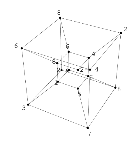
Figure 11: Stereographic projection of the hypercubic parameter space for $\mathrm{Sp(4,\mathbb{R})}/\mathrm{U(2)}$ motions.

A four dimensional hypercube cannot be drawn in three dimension but a standard way to visualize it is provided by presenting its stereographic projection. Indeed if we shift the origin of the coordinate system to the point $\{{\textstyle\frac{1}{2}},{\textstyle\frac{1}{2}},{\textstyle\frac{1}{2}},{\textstyle\frac{1}{2}}\}$ then all the $16$ vertices of the hypercube are located on the standard three-sphere, namely, as $4$-component vectors they have unit norm. So we can consider their stereographic projection from $\mathbb{S}^{3}$ to $\mathbb{R}^{3}$ and connecting them with segments we obtain the visualization of the hypercube displayed in fig.11.

Trapped hypersurfaces

The study of trapped hypersurfaces can now be performed once again in complete analogy with the case of $\mathrm{SL(3,\mathbb{R})}$. We just have to calculate all the relevant minors and impose their vanishing. In this way we determine equations on the parameters that have to be solved within the hypercubic range. If solutions within the hypercube exist, then we have a trapped surface. Otherwise we just have a Weyl replica of an already existing surface. In our case there are just 14 relevant minors distributed in the following way: 4 of rank 1, 4 of rank 3 and 6 of rank 2. Explicitly we can define the following candidate trapped surfaces:

$$\begin{array}[]{rclcl}\Sigma_{1}&:&O_{1,1}&=&0~{},\\ \Sigma_{2}&:&O_{2,1}&=&0~{},\\ \Sigma_{3}&:&O_{3,1}&=&0~{},\\ \Sigma_{4}&:&O_{4,1}&=&0~{},\\ \Sigma_{5}&:&O_{1,3}\left(O_{2,1}O_{3,2}-O_{2,2}O_{3,1}\right)+O_{1,2}\left(O_{2,3}O_{3,1}-O_{2,1}O_{3,3}\right)+O_{1,1}\left(O_{2,2}O_{3,3}-O_{2,3}O_{3,2}\right)&=&0~{},\\ \Sigma_{6}&:&O_{1,3}\left(O_{2,1}O_{4,2}-O_{2,2}O_{4,1}\right)+O_{1,2}\left(O_{2,3}O_{4,1}-O_{2,1}O_{4,3}\right)+O_{1,1}\left(O_{2,2}O_{4,3}-O_{2,3}O_{4,2}\right)&=&0~{},\\ \Sigma_{7}&:&O_{1,3}\left(O_{3,1}O_{4,2}-O_{3,2}O_{4,1}\right)+O_{1,2}\left(O_{3,3}O_{4,1}-O_{3,1}O_{4,3}\right)+O_{1,1}\left(O_{3,2}O_{4,3}-O_{3,3}O_{4,2}\right)&=&0~{},\\ \end{array}$$ (8.40)

$$\begin{array}[]{rclcl}\Sigma_{8}&:&O_{2,3}\left(O_{3,1}O_{4,2}-O_{3,2}O_{4,1}\right)+O_{2,2}\left(O_{3,3}O_{4,1}-O_{3,1}O_{4,3}\right)+O_{2,1}\left(O_{3,2}O_{4,3}-O_{3,3}O_{4,2}\right)&=&0~{},\\ \Sigma_{9}&:&O_{1,1}O_{2,2}-O_{1,2}O_{2,1}&=&0~{},\\ \Sigma_{10}&:&O_{1,1}O_{3,2}-O_{1,2}O_{3,1}&=&0~{},\\ \Sigma_{11}&:&O_{1,1}O_{4,2}-O_{1,2}O_{4,1}&=&0~{},\\ \Sigma_{12}&:&O_{2,1}O_{3,2}-O_{2,2}O_{3,1}&=&0~{},\\ \Sigma_{13}&:&O_{2,1}O_{4,2}-O_{2,2}O_{4,1}&=&0~{},\\ \Sigma_{14}&:&O_{3,1}O_{4,2}-O_{3,2}O_{4,1}&=&0\\ \end{array}$$ (8.41)

where the explicit form of the equation can be obtained by substituting the values of the $\mathrm{U(2)}$ matrix elements as given in eq.s (8.34–8.38). A full-fledged analysis of all the trapped surfaces is beyond the scope of the present paper which aims at illustrating the general principles and at explaining the method. What we can do without any analytic study of the trapped surfaces is to determine the accessible Weyl group elements for each of them and in this way single out the corresponding past infinity and future infinity states. The result is shown in table 6.

$$\begin{array}[]{|c|l|c|l|}\hline\cr\mbox{Surf}&\mbox{Accessible Weyl el.}&\mbox{Flow}&\mbox{Type}\\ \hline\cr\Sigma_{1}&\left\{w_{5},w_{6},w_{3},w_{2},w_{7},w_{8}\right\}&w_{5}\,\ \mapsto\,w_{8}&\mbox{critical}\\ \Sigma_{2}&\left\{w_{1},w_{3},w_{4},w_{2},w_{7},w_{8}\right\}&w_{1}\,\ \mapsto\,w_{8}&\mbox{super-critical}\\ \Sigma_{3}&\left\{w_{5},w_{6},w_{1},w_{3},w_{4},w_{2}\right\}&w_{5}\,\ \mapsto\,w_{2}&\mbox{super-critical}\\ \Sigma_{4}&\left\{w_{5},w_{6},w_{1},w_{4},w_{7},w_{8}\right\}&w_{5}\,\ \mapsto\,w_{8}&\mbox{critical}\\ \Sigma_{5}&\left\{w_{5},w_{6},w_{3},w_{2},w_{7},w_{8}\right\}&w_{5}\,\ \mapsto\,w_{8}&\mbox{critical}\\ \Sigma_{6}&\left\{w_{1},w_{3},w_{4},w_{2},w_{7},w_{8}\right\}&w_{1}\,\ \mapsto\,w_{8}&\mbox{super-critical}\\ \Sigma_{7}&\left\{w_{5},w_{6},w_{1},w_{3},w_{4},w_{2}\right\}&w_{5}\,\ \mapsto\,w_{2}&\mbox{super-critical}\\ \Sigma_{8}&\left\{w_{5},w_{6},w_{1},w_{4},w_{7},w_{8}\right\}&w_{5}\,\ \mapsto\,w_{8}&\mbox{critical}\\ \Sigma_{9}&\left\{w_{6},w_{3},w_{4},w_{2},w_{7},w_{8}\right\}&w_{6}\,\ \mapsto\,w_{8}&\mbox{super-critical}\\ \Sigma_{10}&\left\{w_{5},w_{6},w_{1},w_{3},w_{2},w_{8}\right\}&w_{5}\ \,\mapsto\,w_{8}&\mbox{critical}\\ \Sigma_{11}&\left\{w_{5},w_{6},w_{1},w_{3},w_{4},w_{2},w_{7},w_{8}\right\}&w_{5}\,\ \mapsto\,w_{8}&\mbox{trapped non crit.}\\ \Sigma_{12}&\left\{w_{5},w_{6},w_{1},w_{3},w_{4},w_{2},w_{7},w_{8}\right\}&w_{5}\,\ \mapsto\,w_{8}&\mbox{trapped non crit.}\\ \Sigma_{13}&\left\{w_{5},w_{1},w_{4},w_{2},w_{7},w_{8}\right\}&w_{5}\ \,\mapsto\,w_{8}&\mbox{critical}\\ \Sigma_{14}&\left\{w_{5},w_{6},w_{1},w_{3},w_{4},w_{7}\right\}&w_{5}\ \,\mapsto\,w_{7}&\mbox{super-critical}\\ \hline\cr\end{array}$$

Table 6: Accessible Weyl elements on the $14$ trapped surfaces of $\mathrm{Sp(4,\mathbb{R})/U(2)}$ flows. By inspecting the list $\mathcal{A}_{\Sigma}$ of accessible Weyl elements we easily deduce the character of the surface. If there are missing Weyl elements it is critical. It is super-critical if one of the missing elements is either $\Omega_{min}\,=\,w_{5}$ and/or $\Omega_{max}\,=\,w_{8}$. When no Weyl element is missing in $\mathcal{A}_{\Sigma}$, the surface is just only trapped. It would be critical inside the bigger group $\mathrm{SL(4,\mathbb{R})}$.

As it is evident by inspection of this table the possible flows realized on critical hypersurfaces of parameter space are just a very small number, namely the following five:

$$\begin{array}[]{ccc}1&:&w_{1}\,\mapsto\,w_{8}~{},\\ 2&:&w_{5}\,\mapsto\,w_{2}~{},\\ 3&:&w_{5}\,\mapsto\,w_{7}~{},\\ 4&:&w_{5}\,\mapsto\,w_{8}~{},\\ 5&:&w_{6}\,\mapsto\,w_{8}~{}.\end{array}$$ (8.42)

As we are going to see this is a property shared by the entire universality class of manifolds that have the same Tits Satake projection. The Weyl group, the flow diagram on the links and the possible flows realized on critical surfaces do not depend on the representative inside the class but are just a property of the class.

In the next section we just focus on the detailed discussion of a few examples of flows for this maximally split manifold.

8.4 Examples for $\mathfrak{sp}(4,\mathbb{R})$

In this section, as we just announced, we consider three examples of $\mathrm{Sp(4,\mathbb{R})}$-flows. One will be in the bulk the other two will be located on two different critical surfaces. We analyse these cases in detail both to show the relation between the asymptotic states and the structure of the orthogonal group element $\mathcal{O}$ and to illustrate the billiard phenomenon. In the plots of the Cartan fields we will be able to observe the multiple bouncing of the cosmic ball on the hyperplanes orthogonal to some of the roots.

8.4.1 An example of flow in the bulk of parameter space: $\Omega_{5}\,\Rightarrow\,\Omega_{8}$

If, as initial data we choose the following element of the compact subgroup $\mathrm{U(2)}\subset\mathrm{Sp(4,\mathbb{R})}$:

$$\mathrm{U(2)}\,\ni\,\mathcal{O}\,=\,\exp[{\textstyle\frac{\pi}{6}}\,J_{1}]\,\,\exp[{\textstyle\frac{\pi}{4}}\,J_{2}]\,\,\exp[{\textstyle\frac{\pi}{6}}\,J_{3}]\,\,\exp[{\textstyle\frac{\pi}{3}}\,J_{4}]\,\,$$ (8.43)

$$=\left(\begin{array}[]{llll}\frac{1}{16}\left(6-\sqrt{2}+\sqrt{6}\right)&\frac{\sqrt{\frac{3}{2}}}{4}&\frac{1}{8}\sqrt{3}\left(2+\sqrt{2}\right)&\frac{1}{16}\left(\sqrt{2}-6\sqrt{3}+\sqrt{6}\right)\\ \frac{1}{16}\left(3\sqrt{2}-2\sqrt{3}-\sqrt{6}\right)&\frac{3}{4\sqrt{2}}&\frac{1}{8}\left(-2+3\sqrt{2}\right)&\frac{1}{16}\left(6+3\sqrt{2}+\sqrt{6}\right)\\ \frac{1}{16}\left(-6-3\sqrt{2}-\sqrt{6}\right)&\frac{1}{8}\left(2-3\sqrt{2}\right)&\frac{3}{4\sqrt{2}}&\frac{1}{16}\left(3\sqrt{2}-2\sqrt{3}-\sqrt{6}\right)\\ \frac{1}{16}\left(-\sqrt{2}+6\sqrt{3}-\sqrt{6}\right)&-\frac{1}{8}\sqrt{3}\left(2+\sqrt{2}\right)&\frac{\sqrt{\frac{3}{2}}}{4}&\frac{1}{16}\left(6-\sqrt{2}+\sqrt{6}\right)\\ \end{array}\right)$$

we are just in the bulk. Indeed as it is evident by inspection of eq.(8.43), the $4\times 4$ matrix representing $\mathcal{O}$ has no minor with vanishing determinant. Hence according to the advocated theorems we expect asymptotic sorting of the eigenvalues. Indeed this is what happens. Implementing by numerical evaluation the integration formula on a computer we discover that the asymptotic form of the Lax operator at $t=-\infty$ corresponds to the Weyl group element $\Omega_{5}$

$$\lim_{t\,\rightarrow\,-\infty}\,L(t)\,=\,\left(\begin{array}[]{cccc}2&0&0&0\\ 0&1&0&0\\ 0&0&-1&0\\ 0&0&0&-2\end{array}\right)\,\Leftrightarrow\,\Omega_{5}~{}.$$ (8.48)

Similarly at asymptotically late times the limit of the Lax operator is that corresponding to the Weyl group element $\Omega_{8}$

$$\lim_{t\,\rightarrow\,+\infty}\,L(t)\,=\,\left(\begin{array}[]{cccc}-2&0&0&0\\ 0&-1&0&0\\ 0&0&1&0\\ 0&0&0&2\end{array}\right)\,\Leftrightarrow\,\Omega_{8}~{}.$$ (8.49)

Algebraically we have $\Omega_{8}\,=\,\Omega_{2}\,\Omega_{5}$, so that all generic flows in the bulk that avoid touching critical surfaces are a smooth realization of the Weyl reflection $\Omega_{2}\,\in\,\mathcal{W}$. The particular smooth realization of this reflection provided by the present choice of parameters is illustrated in fig.12 which displays the motion of the cosmic ball on the two dimensional billiard table whose axes are the Cartan fields $h_{1},h_{2}$.

Figure 12: Motion of the cosmic ball on the CSA billiard table of $\mathrm{Sp(4,\mathbb{R})}$ in a generic bulk case. The choice of the angles is $\theta_{1}={\textstyle\frac{\pi}{6}}\,,\,\theta_{2}={\textstyle\frac{\pi}{4}}\,,\,\theta_{3}={\textstyle\frac{\pi}{6}}\,,\,\theta_{4}={\textstyle\frac{\pi}{3}}$. According to theory this motion realizes the smooth reflection $\Omega_{2}$ from the universal primordial Kasner era $\Omega_{5}$ to the universal remote future Kasner era $\Omega_{8}$. This motion involves just two bounces on the wall respectively orthogonal to the root $\alpha_{3}=(1,-1)$ and $\alpha_{1}=(1,1)$. In this picture the straight lines represent the walls orthogonal to $\alpha_{1}$ and $\alpha_{3}$, respectively.

This motion involves two bounces as it becomes evident by plotting the projection of the Cartan vector $\overrightarrow{h}=\left(h_{1},h_{2}\right)$ along the two roots $\alpha_{1}=(1,-1)$ and $\alpha_{3}=(1,1)$. These plots are displayed in fig.13.

Figure 13: Plot of ${\alpha}_{1,3}\cdot h$ projections for the $\mathrm{Sp(4,\mathbb{R})}$ generic bulk flow generated by the parameter choice $\theta_{1}={\textstyle\frac{\pi}{6}}\,,\,\theta_{2}={\textstyle\frac{\pi}{4}}\,,\,\theta_{3}={\textstyle\frac{\pi}{6}}\,,\,\theta_{4}={\textstyle\frac{\pi}{3}}$which connects the primordial Kasner era $\Omega_{5}$ to the remote future Kasner era $\Omega_{8}$. There are two bounces in this flow because the projections ${\alpha_{1,3}}\cdot h$ have maxima at different instant of times.

8.4.2 An example of flow on the super-critical surface $\Sigma_{9}$: $\Omega_{6}\,\Rightarrow\,\Omega_{8}$

As a next example we consider a flow confined on a super-critical surface. If we set $\theta_{2}=\frac{\pi}{2}$ the $\mathrm{U(2)}$ matrix takes the following form:

$$\mathcal{O} = \left(\begin{array}[]{llll}\cos\left(\theta_{1}+\theta_{3}\right)\cos\left(\theta_{4}\right)&0&\sin\left(\theta_{1}+\theta_{3}\right)&-\cos\left(\theta_{1}+\theta_{3}\right)\sin\left(\theta_{4}\right)\\ -\cos\left(\theta_{4}\right)\sin\left(\theta_{1}+\theta_{3}\right)&0&\cos\left(\theta_{1}+\theta_{3}\right)&\sin\left(\theta_{1}+\theta_{3}\right)\sin\left(\theta_{4}\right)\\ -\sin\left(\theta_{1}+\theta_{3}\right)\sin\left(\theta_{4}\right)&-\cos\left(\theta_{1}+\theta_{3}\right)&0&-\cos\left(\theta_{4}\right)\sin\left(\theta_{1}+\theta_{3}\right)\\ \cos\left(\theta_{1}+\theta_{3}\right)\sin\left(\theta_{4}\right)&-\sin\left(\theta_{1}+\theta_{3}\right)&0&\cos\left(\theta_{1}+\theta_{3}\right)\cos\left(\theta_{4}\right)\end{array}\right)$$ (8.54)

which has two notable properties. The first is that it has vanishing some principal minors, the second is that it actually depends on two variables only, namely $\theta_{1}\,+\,\theta_{3}$ and $\theta_{4}$.

If we consider the equation for the critical super-surface $\Sigma_{9}$ we find

$$\cos\left(\theta_{2}\right)\cos^{2}\left(\theta_{3}\right)\cos\left(\theta_{4}\right)\,=\,0$$ (8.56)

so that the hyperplane $\theta_{2}=\frac{\pi}{2}$ where we have chosen our group element is just one of the three components of $\Sigma_{9}$. Furthermore, because of what we just observed, on this hyperplane all points of the following form have to be identified:

$$\forall\,\phi\,\in\left[0,{\textstyle\frac{\pi}{2}}\right]\,;\,\left(\theta_{1}+\phi,\frac{\pi}{2},\theta_{3}-\phi,\theta_{4}\right)\,\sim\,\left(\theta_{1},\frac{\pi}{2},\theta_{3},\theta_{4}\right)~{}.$$ (8.57)

Having chosen initial data on a trapped surface, namely $\Sigma_{9}$, we do not expect full asymptotic sorting of the eigenvalues: actually, according to table 6 we expect flows from $\Omega_{6}$ to $\Omega_{8}$. Indeed this is what happens. We verify it in one example. For instance, as initial data we choose the following element of the compact subgroup $\mathrm{U(2)}\subset\mathrm{Sp(4,\mathbb{R})}$, which lies in the considered hypersurface:

$$\mathrm{U(2)}\,\ni\,\mathcal{O} = \exp[{\textstyle\frac{\pi}{3}}\,J_{1}]\,\exp[{\textstyle\frac{\pi}{2}}\,J_{2}]\,\,\exp[{\textstyle\frac{\pi}{3}}\,J_{3}]\,\exp[{\textstyle\frac{\pi}{3}}\,J_{4}]$$ (8.62)

$$= \left(\begin{array}[]{llll}-\frac{1}{4}&0&\frac{\sqrt{3}}{2}&\frac{\sqrt{3}}{4}\\ -\frac{\sqrt{3}}{4}&0&-\frac{1}{2}&\frac{3}{4}\\ -\frac{3}{4}&\frac{1}{2}&0&-\frac{\sqrt{3}}{4}\\ -\frac{\sqrt{3}}{4}&-\frac{\sqrt{3}}{2}&0&-\frac{1}{4}\end{array}\right)~{}.$$

Implementing by numerical evaluation the integration formula on a computer we discover that the asymptotic form of the Lax operator at $t=-\infty$ corresponds to the Weyl group element $\Omega_{6}$ which implies no decreasing sorting of the eigenvalues

$$\lim_{t\,\rightarrow\,-\infty}\,L(t)\,=\,\left(\begin{array}[]{cccc}2&0&0&0\\ 0&-1&0&0\\ 0&0&1&0\\ 0&0&0&-2\end{array}\right)\,\Leftrightarrow\,\Omega_{6}~{}.$$ (8.63)

On the other hand the limit of the Lax operator at asymptotically late times is that corresponding to the Weyl group element $\Omega_{8}$ which is the same occurring in generic flows and yields increasing sorting of the eigenvalues

$$\lim_{t\,\rightarrow\,+\infty}\,L(t)\,=\,\left(\begin{array}[]{cccc}-2&0&0&0\\ 0&-1&0&0\\ 0&0&1&0\\ 0&0&0&2\end{array}\right)\,\Leftrightarrow\,\Omega_{8}~{}.$$ (8.64)

Algebraically we have $\Omega_{8}\,=\,\Omega_{3}\,\Omega_{6}$, so that the flows occurring on this super-critical surface are smooth realizations of the Weyl reflection $\Omega_{3}\,\in\,\mathcal{W}$. The particular smooth realization of this reflection encoded in this flow is illustrated in fig.14 which displays the motion of the cosmic ball on the two dimensional billiard table

Figure 14: Motion of the cosmic ball on the CSA billiard table of $\mathrm{Sp(4,\mathbb{R})}$ in a super-critical surface case. The choice of the angles is $\theta_{1}={\textstyle\frac{\pi}{3}}\,,\,\theta_{2}={\textstyle\frac{\pi}{2}}\,,\,\theta_{3}={\textstyle\frac{\pi}{3}}\,,\,\theta_{4}={\textstyle\frac{\pi}{3}}$. This motion realizes the smooth reflection $\Omega_{3}$ from the Kasner era $\Omega_{6}$ at $t=-\infty$ to the Kasner era $\Omega_{8}$ at $t=+\infty$. The two straight lines appearing in the picture are the walls orthogonal to the roots $\alpha_{2}=(0,2)$ and $\alpha_{4}=(2,0)$, respectively. As one sees the cosmic ball just bounces once the on the $\alpha_{4}$ wall.

This motion involves just one bounce on the wall orthogonal to the root $\alpha_{4}$ as it becomes evident by inspecting fig.15.

Figure 15: Plot of ${\alpha}_{2,4}\cdot h$ projections for the $\mathrm{Sp(4,\mathbb{R})}$ flow on a super-critical surface generated by the parameter choice $\theta_{1}={\textstyle\frac{\pi}{3}}\,,\,\theta_{2}={\textstyle\frac{\pi}{2}}\,,\,\theta_{3}={\textstyle\frac{\pi}{3}}\,,\,\theta_{4}={\textstyle\frac{\pi}{3}}$ which connects the past Kasner era $\Omega_{6}$ to the future Kasner era $\Omega_{8}$. There is just one bounce in this flow and this occurs on the $\alpha_{4}$ wall.

8.4.3 An example of flow on the super-critical surface $\Sigma_{2}$: $\Omega_{1}\,\Rightarrow\,\Omega_{8}$

In the example considered below the initial state is different from that appearing in a generic bulk flow, namely there is not decreasing sorting of the eigenvalues at past infinity which rather corresponds to the Weyl element $\Omega_{1}$. Yet the end point at $t=+\infty$ coincides with the universal one $\Omega_{8}$, namely there is increasing sorting at future infinity. We realize this situation by choosing initial data on one of the critical surfaces, namely the surface $\Sigma_{2}$.

The equation for the trapped surface $\Sigma_{2}$, as defined in (8.40) reads as follows:

$$0\,=\,\cos\left(\theta_{3}\right)\cos\left(\theta_{4}\right)\sin\left(\theta_{1}\right)+\cos\left(\theta_{1}\right)\sin\left(\theta_{3}\right)\sin\left(\theta_{2}-\theta_{4}\right)$$ (8.65)

and it can be solved within the hypercube by expressing $\theta_{1}$ in terms of the remaining three Euler angles as it follows:

$$\theta_{1}\,=\,\arccos\left(\frac{\cos\left(\theta_{3}\right)\cos\left(\theta_{4}\right)}{\sqrt{\cos^{2}\left(\theta_{3}\right)\cos^{2}\left(\theta_{4}\right)+\sin^{2}\left(\theta_{3}\right)\sin^{2}\left(\theta_{2}-\theta_{4}\right)}}\right)~{}.$$ (8.66)

On the hypersurface $\Sigma_{2}$ we choose the particularly nice point

$$\left\{\frac{\pi}{3},\frac{\pi}{6},\frac{\pi}{3},\frac{\pi}{3}\right\}\,\in\,\Sigma_{2}$$ (8.67)

which is easily seen to verify the defining equation (8.65) and which leads to a quite simple form of the matrix $\mathcal{O}$. With these values of the Euler angles we obtain the following element of the maximally compact subgroup $\mathrm{U(2)}\subset\mathrm{Sp(4,\mathbb{R})}$:

$$\mathrm{U(2)}\,\ni\,H_{sp} = \exp[{\textstyle\frac{\pi}{3}}\,J_{1}]\,\exp[{\textstyle\frac{\pi}{6}}\,J_{2}]\,\,\exp[{\textstyle\frac{\pi}{3}}\,J_{3}]\,\exp[{\textstyle\frac{\pi}{3}}\,J_{4}]$$ (8.72)

$$= \left(\begin{array}[]{llll}\frac{1}{2}&\frac{3}{8}&\frac{3\sqrt{3}}{8}&\frac{\sqrt{3}}{4}\\ 0&\frac{\sqrt{3}}{8}&-\frac{5}{8}&\frac{3}{4}\\ -\frac{3}{4}&\frac{5}{8}&\frac{\sqrt{3}}{8}&0\\ -\frac{\sqrt{3}}{4}&-\frac{3\sqrt{3}}{8}&\frac{3}{8}&\frac{1}{2}\end{array}\right)$$

which indeed has vanishing $O_{2,1}$ matrix element as it is required by the definition of the $\Sigma_{2}$ trapped surface. Hence according to table 6 we expect a flow from $\Omega_{1}$ to $\Omega_{8}$. Before proceeding to the integration of the Lax equation it is interesting to consider the $\mathfrak{so}(2,3)$ 5-dimensional representation of the same $\mathrm{U(2)}$ group element. It is explicitly given by the following matrix:

$$H_{so}\,=\,\left(\begin{array}[]{lllll}\frac{\sqrt{3}}{16}&\frac{5}{16}&-\frac{3}{4\sqrt{2}}&-\frac{3}{16}&-\frac{7\sqrt{3}}{16}\\ -\frac{19}{32}&\frac{11\sqrt{3}}{32}&\frac{3\sqrt{\frac{3}{2}}}{8}&-\frac{5\sqrt{3}}{32}&-\frac{3}{32}\\ \frac{3\sqrt{\frac{3}{2}}}{16}&\frac{15}{16\sqrt{2}}&-\frac{1}{8}&\frac{15}{16\sqrt{2}}&\frac{3\sqrt{\frac{3}{2}}}{16}\\ -\frac{3}{32}&-\frac{5\sqrt{3}}{32}&\frac{3\sqrt{\frac{3}{2}}}{8}&\frac{11\sqrt{3}}{32}&-\frac{19}{32}\\ -\frac{7\sqrt{3}}{16}&-\frac{3}{16}&-\frac{3}{4\sqrt{2}}&\frac{5}{16}&\frac{\sqrt{3}}{16}\end{array}\right)~{}.$$ (8.73)

Since all the properties of the flows are intrinsic properties of the group and cannot depend on the chosen representation it follows that also the matrix (8.73) should be critical namely some of its relevant minors (those obtained by intesecting the first $k$-columns with $k$ arbitrary rows should vanish. Although not evident at first sight, this is indeed true. Calculating the minors we find that there are three relevant $2\times 2$ minors whose determinant vanishes, namely

$$\mbox{Det}\,\left(\begin{array}[]{ll}\frac{\sqrt{3}}{16}&\frac{5}{16}\\ \frac{3\sqrt{\frac{3}{2}}}{16}&\frac{15}{16\sqrt{2}}\end{array}\right) = 0\quad;\quad\,\mbox{Det}\,\left(\begin{array}[]{ll}\frac{\sqrt{3}}{16}&\frac{5}{16}\\ -\frac{3}{32}&-\frac{5\sqrt{3}}{32}\end{array}\right)\,=\,0~{},$$ (8.78)

$$\mbox{Det}\left(\begin{array}[]{ll}\frac{3\sqrt{\frac{3}{2}}}{16}&\frac{15}{16\sqrt{2}}\\ -\frac{3}{32}&-\frac{5\sqrt{3}}{32}\end{array}\right) = 0~{}.$$ (8.81)

Hence the criticality condition is indeed intrinsic to the choice of the group element and not to its specific representation as a matrix.

Implementing by numerical evaluation the integration formula on a computer we discover that the asymptotic form of the Lax operator at $t=-\infty$ corresponds to the Weyl group element $\Omega_{1}$ as expected:

$$\lim_{t\,\rightarrow\,-\infty}\,L(t)\,=\,\left(\begin{array}[]{cccc}1&0&0&0\\ 0&2&0&0\\ 0&0&-2&0\\ 0&0&0&-12\end{array}\right)\,\Leftrightarrow\,\Omega_{1}$$ (8.82)

while the limit at asymptotically late times is that corresponding to the Weyl group element $\Omega_{8}$ as we also expected

$$\lim_{t\,\rightarrow\,+\infty}\,L(t)\,=\,\left(\begin{array}[]{cccc}-2&0&0&0\\ 0&-1&0&0\\ 0&0&1&0\\ 0&0&0&2\end{array}\right)\,\Leftrightarrow\,\Omega_{8}~{}.$$ (8.83)

Algebraically we have $\Omega_{8}\,=\,\Omega_{8}\,\Omega_{1}$, so that the flows occurring on this super-critical surface are smooth realizations of the Weyl reflection $\Omega_{8}\,\in\,\mathcal{W}$. The smooth realization of this reflection encoded in the flow with these initial data is illustrated in fig.16 which displays the motion of the cosmic ball in the $h_{1},h_{2}$ Cartan subalgebra plane.

Figure 16: Motion of the cosmic ball on the CSA billiard table of $\mathrm{Sp(4,\mathbb{R})}$ in a super-critical surface case. The choice of the angles is $\theta_{1}={\textstyle\frac{\pi}{3}}\,,\,\theta_{2}={\textstyle\frac{\pi}{6}}\,,\,\theta_{3}={\textstyle\frac{\pi}{3}}\,,\,\theta_{4}={\textstyle\frac{\pi}{3}}$ which lie on the trapped and super-critical surface $\Sigma_{2}$. This motion realizes the smooth reflection $\Omega_{8}$ from the Kasner era $\Omega_{1}$ at $t=-\infty$ to the Kasner era $\Omega_{8}$ at $t=+\infty$. The peculiar knot appearing in this picture implies the existence of two bounces on the same root wall. The two straight lines displayed in the figure are the walls orthogonal to the two simple roots $\alpha_{1}=(1,-1)$ and $\alpha_{2}=(0,2)$. The ball bounces twice on the $\alpha_{1}$ wall.

This motion involves three bounces two on the wall orthogonal to the simple root $\alpha_{1}$ and one on the wall orthogonal to $\alpha_{2}$. This is clearly visible by inspection of fig.17.

Figure 17: Plot of ${\alpha}_{1,2}\cdot h$ projections for the $\mathrm{Sp(4,\mathbb{R})}$ flow on a super-critical surface generated by the parameter choice $\theta_{1}={\textstyle\frac{\pi}{3}}\,,\,\theta_{2}={\textstyle\frac{\pi}{6}}\,,\,\theta_{3}={\textstyle\frac{\pi}{3}}\,,\,\theta_{4}={\textstyle\frac{\pi}{3}}$ which connects the past Kasner era $\Omega_{1}$ to the future Kasner era $\Omega_{8}$. The two bounces are clearly visible in the maxima and minima of the first graph.

9 The case of the $\mathfrak{so}(r,r+2s)$ algebra

We are interested in considering the sigma model on the symmetric non compact coset manifold

$$\mathcal{M}_{(r,2s)}\,=\,\frac{\mathrm{SO(r,r+2s)}}{\mathrm{SO(r)}\times\mathrm{SO(r+2s)}}~{}.$$ (9.1)

For $r=4$ the above manifold is quaternionic and corresponds to the family of special geometries $L(0,P=2s)$.

Figure 18: The Dynkin diagram of the $D_{\ell}$ Lie algebra.

9.1 The corresponding complex Lie algebra and root system

The complex Lie algebra of which $\mathfrak{so}(r,r+2s)$ is a non-compact real section is just $D_{\ell}$ where

$$\ell=r+s~{}.$$ (9.2)

The corresponding Dynkin diagram is displayed in fig 18 and the associated root system is realized by the following set of vectors in $\mathbb{R}^{\ell}$:

$$\Delta\equiv\left\{\pm\,\epsilon^{A}\,\pm\epsilon^{B}\right\}\quad;\quad\mbox{card}\,\Delta\,=\,2\left(\ell^{2}\,-\,\ell\right)$$ (9.3)

where $\epsilon^{A}$ denotes an orthonormal basis of unit vectors. The set of positive roots is then easily defined as follows:

$$\alpha\,>\,0\quad\Rightarrow\,\alpha\,\in\,\Delta_{+}\,\equiv\,\left\{\epsilon^{A}\,\pm\epsilon^{B}\right\}\quad(A<B)~{}.$$ (9.4)

A standard basis of simple roots representing the Dynkin diagram 18 is given by

$$\alpha_{1} = \epsilon_{1}\,-\,\epsilon_{2}~{},$$

$$\alpha_{2} = \epsilon_{2}\,-\,\epsilon_{3}~{},$$

$$\dots \dots \dots~{},$$

$$\alpha_{\ell-1} = \epsilon_{\ell-1}\,-\,\epsilon_{\ell}~{},$$

$$\alpha_{\ell} = \epsilon_{\ell-1}\,+\,\epsilon_{\ell}~{}.$$ (9.5)

The maximally split real form of the $D_{\ell}$ Lie algebra is $\mathfrak{so}(\ell,\ell)$ and it is explicitly realized by the following $2\ell\times 2\ell$ matrices. Let $e_{A,B}$ denote the $2\ell\times 2\ell$ matrix whose entries are all zero except the entry $A,B$ which is equal to one. Then the Cartan generators $\mathcal{H}_{A}$ and the positive root step operators $E^{\alpha}$ are represented as follows:

$$\mathcal{H}_{A} = e_{A,A}\,-\,e_{A+\ell,A+\ell}~{},$$

$$E^{\epsilon_{A}\,-\,\epsilon_{B}} = e_{B,A}\,-\,e_{A+\ell,B+\ell}~{},$$

$$E^{\epsilon_{A}\,+\,\epsilon_{B}} = e_{A+\ell,B}\,-\,e_{B+\ell,A}~{}.$$ (9.6)

The solvable algebra of the maximally split coset

$$\mathcal{M}_{(\ell,0)}\,=\,\frac{\mathrm{SO(\ell,\ell)}}{\mathrm{SO(\ell)}\times\mathrm{SO(\ell)}}$$ (9.7)

has therefore a very simple form in terms of matrices. Following the general constructive principles $Solv_{(\ell,\ell)}$ is just the algebraic span of all the matrices (9.6) so that

$$Solv_{(\ell,\ell)}\,\ni\,M\,\Leftrightarrow\,M\,=\,\left(\begin{array}[]{c|c}T&B\\ \hline\cr 0&-T^{T}\end{array}\right)\quad;\quad\left\{\begin{array}[]{rcl}T&=&\mbox{upper triangular}~{},\\ B&=&-\,B^{T}\quad\mbox{antisymmetric.}\end{array}\right.$$ (9.8)

The matrices of the form (9.8) clearly form a subalgebra of the $\mathfrak{so}(\ell,\ell)$ algebra which, in this representation, is defined as the set of matrices $\Lambda$ fulfilling the following condition:

$$\Lambda^{T}\,\left(\begin{array}[]{c|c}0&\mathbf{1}_{l}\\ \hline\cr\mathbf{1}_{l}&0\end{array}\right)\,+\,\left(\begin{array}[]{c|c}0&\mathbf{1}_{l}\\ \hline\cr\mathbf{1}_{l}&0\end{array}\right)\Lambda\,=\,0~{}.$$ (9.9)

9.2 The real form $\mathfrak{so}(r,r+2s)$ of the $D_{r+s}$ Lie algebra

The main point in order to apply to the coset manifold (9.1) the general integration algorithm of the Lax equation devised for the case $\mathrm{SL(2\ell)}/\mathrm{SO(2\ell)}$ consists of introducing a convenient basis of generators of the Lie algebra $\mathfrak{so}(r,r+2s)$ where, in the fundamental representation, all elements of the solvable Lie algebra associated with the coset under study turn out to be given by upper triangular matrices. With some ingenuity such a basis can be found by defining the $\mathfrak{so}(r,r+2s)$ Lie algebra as the set of matrices $\Lambda_{t}$ satisfying the following constraint:

$$\Lambda_{t}^{T}\,\eta_{t}\,+\,\eta_{t}\,\Lambda_{t}\,=\,0$$ (9.10)

where the symmetric invariant metric $\eta_{t}$ with $r+2s$ positive eigenvalues $(+1)$ and $r$ negative ones $(-1)$ is given by the following matrix.

$$\eta_{t}\,=\,\left(\begin{array}[]{c|c|c}0&0&\varpi_{r}\\ \hline\cr 0&\mathbf{1}_{2s}&0\\ \hline\cr\varpi_{r}&0&0\end{array}\right)~{}.$$ (9.11)

In the above equation the symbol $\varpi_{r}$ denotes the completely anti-diagonal $r\times r$ matrix which follows:

$$\varpi_{r}\,=\,\left.\underbrace{\left(\begin{array}[]{cccccc}0&0&\dots&\dots&0&1\\ 0&0&\dots&\dots&1&0\\ 0&0&\dots&1&0&0\\ \dots&\dots&\dots&\dots&\dots&\dots\\ 0&1&0&\dots&\dots&0\\ 1&0&0&\dots&\dots&0\end{array}\right)}_{r}\right\}\,r~{}.$$ (9.12)

Obviously there is a simple orthogonal transformation which maps the metric $\eta_{t}$ into the standard block diagonal metric $\eta_{b}$ written below

$$\eta_{b}\,=\,\left(\begin{array}[]{c|c|c}\mathbf{1}_{r}&0&0\\ \hline\cr 0&\mathbf{1}_{2s}&0\\ \hline\cr 0&0&-\mathbf{1}_{r}\end{array}\right)~{}.$$ (9.13)

Indeed we can write

$$\Omega^{T}\,\eta_{b}\,\Omega\,=\,\eta_{t}$$ (9.14)

where the explicit form of the matrix $\Omega$ is the following:

$$\Omega\,=\,\left(\begin{array}[]{c|c|c}0&\mathbf{1}_{2s}&0\\ \hline\cr{\textstyle\frac{1}{\sqrt{2}}}\,\mathbf{1}_{r}&0&{\textstyle\frac{1}{\sqrt{2}}}\varpi_{r}\\ \hline\cr{\textstyle\frac{1}{\sqrt{2}}}\,\mathbf{1}_{r}&0&-{\textstyle\frac{1}{\sqrt{2}}}\varpi_{r}\end{array}\right)~{}.$$ (9.15)

Correspondingly the orthogonal transformation $\Omega$ maps the Lie algebra and group elements of $\mathfrak{so}(r,r+2s)$ from the standard basis where the invariant metric is $\eta_{b}$ to the basis where it is $\eta_{t}$

$$\Lambda_{t}\,=\,\Omega^{T}\,\Lambda_{b}\,\Omega\,.$$ (9.16)

In the $t$-basis the general form of an element of the solvable Lie algebra which generates the coset manifold (9.1) has the following appearance:

$$Solv\left(\frac{\mathrm{SO(r,r+2s)}}{\mathrm{SO(r)}\times\mathrm{SO(r+2s)}}\right)\,\ni\,\Lambda_{t} = \left(\begin{array}[]{c|c|c}T&X&B\\ \hline\cr 0&0&X^{T}\,\varpi_{r}\\ \hline\cr 0&0&-\varpi_{r}\,T^{T}\,\varpi_{r}\end{array}\right)$$ (9.20)

where

$$T = \left(\begin{array}[]{cccccc}T_{1,1}&T_{1,2}&\dots&\dots&T_{1,r-1}&T_{1,r}\\ 0&T_{2,2}&\dots&\dots&T_{2,r-1}&T_{2,r}\\ 0&0&T_{3,3}&\dots&\dots&T_{3,r}\\ \dots&\dots&\dots&\dots&\dots&\dots\\ 0&0&0&\dots&T_{r-1,r-1}&T_{r-1,r}\\ 0&0&0&\dots&\dots&T_{r,r}\end{array}\right)\,\quad\,\mbox{upper triangular $r\times r$~{},}$$ (9.27)

$$B = -B^{T}\,\quad\,\mbox{antisymmetric $r\times r$~{},}$$

$$X = r\times 2s$$ arbitrary (9.28)

while an element of the maximal compact subalgebra has instead the following appearance:

$$\mathfrak{so}(r)\,\oplus\,\mathfrak{so}(r+2s)\,\ni\,\Lambda_{t} = \left(\begin{array}[]{c|c|c}Z&Y&C\,\varpi_{r}\\ \hline\cr-Y^{T}&Q&-\,Y^{T}\,\varpi_{r}\\ \hline\cr\varpi_{r}\,C&\varpi_{r}Y&-\varpi_{r}\,Z^{T}\,\varpi_{r}\end{array}\right)$$ (9.32)

where

$$Z = -\,Z^{T}\,\mbox{antisymmetric $r\times r$}~{},$$

$$C = -\,C^{T}\,\mbox{antisymmetric $r\times r$}~{},$$

$$Q = -\,Q^{T}\,\mbox{antisymmetric $2s\times 2s$}~{}.$$

$$Y = r\times 2s$$ arbitrary (9.33)

Having clarified the structure of the matrices representing Lie algebra elements in this basis well adapted to the Tits Satake projection, we can now discuss a basis of generators also well adapted to the same projection. To this effect, let us denote by $\mathcal{I}_{ij}$ the $r\times r$ matrices whose only non vanishing entry is the $ij$-th one which is equal to $1$

$$\mathcal{I}_{ij}\,=\,\left(\begin{array}[]{ccccccl}0&0&\dots&\dots&\dots&0&\hbox{}\\ 0&0&\dots&\dots&\dots&0&\hbox{}\\ \dots&\dots&\dots&\dots&\dots&\dots&\hbox{}\\ 0&0&\dots&1&\dots&0&\}\,\mbox{i-th row}\\ 0&0&\dots&\dots&\dots&0\\ 0&0&\dots&\underbrace{\dots}_{\mbox{j-th column}}&\dots&0&\hbox{}\end{array}\right)~{}.$$ (9.34)

Using this notation the $r$ non-compact Cartan generators are given by

$$\mathcal{H}_{i}\,=\,\left(\begin{array}[]{c|c|c}\mathcal{I}_{ii}&0&0\\ \hline\cr 0&0&0\\ \hline\cr 0&0&-\varpi_{r}\,\mathcal{I}_{ii}\,\varpi_{r}\end{array}\right)\,\quad;\quad\,(i=1,\dots,r)~{}.$$ (9.35)

Next we introduce the coset generators associated with the long roots of type: $\alpha=\epsilon^{i}-\epsilon^{j}$.

$$\begin{array}[]{c}\mbox{\scriptsize{$\alpha=\epsilon^{i}-\epsilon^{j}$ }}\\ \mbox{\scriptsize{ $i<j=1,\dots,r$}}\end{array} \Rightarrow K^{ij}_{-}={\textstyle\frac{1}{\sqrt{2}}}\,\left(E^{\alpha}+E^{-\alpha}\right)={\textstyle\frac{1}{\sqrt{2}}}\left(\begin{array}[]{c|c|c}\mathcal{I}_{ij}+\mathcal{I}_{ji}&0&0\\ \hline\cr 0&0&0\\ \hline\cr 0&0&-\varpi_{r}\,\left(\mathcal{I}_{ij}+\mathcal{I}_{ji}\right)\,\varpi_{r}\end{array}\right)$$ (9.41)

and the coset generators associated with the long roots of type $\alpha=\epsilon^{i}+\epsilon^{j}$:

$$\begin{array}[]{c}\mbox{\scriptsize{$\alpha=\epsilon^{i}+\epsilon^{j}$ }}\\ \mbox{\scriptsize{ $i<j=1,\dots,r$}}\end{array} \Rightarrow K^{ij}_{+}={\textstyle\frac{1}{\sqrt{2}}}\,\left(E^{\alpha}+E^{-\alpha}\right)={\textstyle\frac{1}{\sqrt{2}}}\left(\begin{array}[]{c|c|c}0&0&\left(\mathcal{I}_{ij}-\mathcal{I}_{ji}\right)\varpi_{r}\\ \hline\cr 0&0&0\\ \hline\cr\varpi_{r}\left(\mathcal{I}_{ji}-\mathcal{I}_{ij}\right)&0&0\end{array}\right)~{}.$$ (9.48)

The short roots, after the Tits-Satake projection, are just $r$, namely $\epsilon^{i}$. Each of them, however, appears with multiplicity $2s$, due to the paint group. We introduce a $2s$-tuple of coset generators associated to each of the short roots in such a way that such $2s$-tuple transforms in the fundamental representation of $\mathbf{G}_{paint}\,=\,\mathfrak{so}(2s)$. To this effect let us define the rectangular $r\times 2s$ matrices$\mathcal{J}_{im}$ analogous to the square matrices $\mathcal{I}_{ij}$, namely

$$\mathcal{J}_{im}\,=\,\left(\begin{array}[]{ccccccccl}0&0&\dots&\dots&\dots&\dots&\dots&0&\hbox{}\\ 0&0&\dots&\dots&\dots&\dots&\dots&0&\hbox{}\\ \dots&\dots&\dots&\dots&\dots&\dots\dots&\dots&\hbox{}\hfil\\ 0&0&\dots&1&\dots&\dots&\dots&0&\}\,\mbox{i-th row}\\ 0&0&\dots&\dots&\dots&\dots&\dots&0\\ 0&0&\dots&\underbrace{\dots}_{\mbox{$m$-th column}}&\dots&\dots&\dots&0&\hbox{}\end{array}\right)~{}.$$ (9.50)

Then we introduce the following coset generators:

$$\begin{array}[]{c}\mbox{\scriptsize{$\alpha=\epsilon^{i}$ }}\\ \mbox{\scriptsize{ $i=1,\dots,r$}}\\ \mbox{\scriptsize{ $m=1,\dots,2s$}}\\ \end{array} \Rightarrow K^{i}_{m}={\textstyle\frac{1}{\sqrt{2}}}\left(\begin{array}[]{c|c|c}0&\mathcal{J}_{im}&0\\ \hline\cr\mathcal{J}_{im}^{T}&0&-\mathcal{J}_{im}^{T}\,\varpi_{r}\\ \hline\cr 0&-\varpi_{r}\,\mathcal{J}_{im}&0\end{array}\right)~{}.$$ (9.57)

The remaining generators of the $\mathfrak{so}(r,r+2s)$ algebra are all compact and span the subalgebra $\mathfrak{so}(r)\oplus\mathfrak{so}(r+2s)\subset\mathfrak{so}(r,r+2s)$. According to the nomenclature of eq.(9.32) we introduce four sets of generators. The first set is associated with the long roots of type $\alpha=\epsilon^{i}-\epsilon^{j}$ and is defined as follows:

$$Z^{ij}\,=\,{\textstyle\frac{1}{\sqrt{2}}}\,\left(E^{\alpha}-E^{-\alpha}\right)={\textstyle\frac{1}{\sqrt{2}}}\left(\begin{array}[]{c|c|c}\mathcal{I}_{ij}-\mathcal{I}_{ji}&0&0\\ \hline\cr 0&0&0\\ \hline\cr 0&0&-\varpi_{r}\,\left(\mathcal{I}_{ij}-\mathcal{I}_{ji}\right)\,\varpi_{r}\end{array}\right)~{}.$$ (9.59)

The second set is associated with the long roots of type $\alpha=\epsilon^{i}+\epsilon^{j}$ and is defined as follows:

$$C^{ij}={\textstyle\frac{1}{\sqrt{2}}}\,\left(E^{\alpha}-E^{-\alpha}\right)={\textstyle\frac{1}{\sqrt{2}}}\left(\begin{array}[]{c|c|c}0&0&\left(\mathcal{I}_{ij}-\mathcal{I}_{ji}\right)\varpi_{r}\\ \hline\cr 0&0&0\\ \hline\cr-\varpi_{r}\left(\mathcal{I}_{ji}-\mathcal{I}_{ij}\right)&0&0\end{array}\right)~{}.$$ (9.60)

The third group of compact generators spans the compact coset

$$\frac{\mathrm{SO(r+2s)}}{\mathrm{SO(r)}\times\mathrm{SO(2s)}}$$ (9.61)

and it is given by

$$Y^{i}_{m}={\textstyle\frac{1}{\sqrt{2}}}\left(\begin{array}[]{c|c|c}0&\mathcal{J}_{im}&0\\ \hline\cr-\mathcal{J}_{im}^{T}&0&-\mathcal{J}_{im}^{T}\,\varpi_{r}\\ \hline\cr 0&\varpi_{r}\,\mathcal{J}_{im}&0\end{array}\right)~{}.$$ (9.62)

The fourth set of compact generators spans the paint group Lie algebra $\mathfrak{so}(2s)$ and is given by

$$Q_{mn}\,=\,\left(\begin{array}[]{c|c|c}0&0&0\\ \hline\cr 0&\mathcal{Q}_{mn}-\mathcal{Q}_{nm}&0\\ \hline\cr 0&0&0\end{array}\right)$$ (9.63)

where $\mathcal{Q}_{mn}$ denotes the analogue of the $\mathcal{I}_{ij}$ in $2s$ rather than in $r$ dimensions.

By performing the change of basis to the block diagonal form of the matrices we can verify that $C_{ij}-Z_{ij}$ generate the $\mathfrak{so}(r)$ subalgebra while $C_{ij}+Z_{ij}$ together with $Q_{mn}$ and $Y_{im}$ generate the subalgebra $\mathfrak{so}(r+2s)$.

The full set of generators is ordered in the following way:

$$T_{\Lambda}\,=\,\left\{\underbrace{\mathcal{H}_{i}}_{r}\,,\,\underbrace{K^{ij}_{-}}_{{\textstyle\frac{1}{2}}r(r-1)}\,,\,\underbrace{K^{ij}_{+}}_{{\textstyle\frac{1}{2}}r(r-1)}\,,\,\underbrace{K^{i}_{m}}_{2rs}\,,\,\underbrace{Z^{ij}}_{{\textstyle\frac{1}{2}}r(r-1)}\,,\,\underbrace{C^{ij}}_{{\textstyle\frac{1}{2}}r(r-1)}\,,\,\underbrace{Y^{i}_{m}}_{2rs}\,,\,\underbrace{Q_{mn}}_{s(2s-1)}\right\}$$ (9.64)

and satisfy the trace relation:

$$\mbox{Tr}\,\left(T_{\Lambda}\,T_{\Sigma}\right) = g_{\Lambda\Sigma}~{},$$

$$g_{\Lambda\Sigma} = 2\,\mbox{diag}\left(\underbrace{+,+,\dots,+}_{r(r+2s)},\underbrace{-,-,\dots,-}_{r^{2}-r+2rs+2s^{2}-s}\right)~{}.$$ (9.65)

In this way we have obtained the needed and detailed construction of the embedding (6.1) which is necessary to apply the integration algorithm. In the next section we make a detailed study of the case $r=2,s=1$.

10 A case study for the Tits Satake projection: $\mathrm{SO(2,4)}$

The simplest example of not maximally split manifold inside the series defined by eq.(9.1) corresponds to the choice: $r=2,\,s=1$, namely

$$\mathcal{M}_{2,2}\,\equiv\,\frac{\mathrm{SO(2,4)}}{\mathrm{SO(2)\times SO(4)}}~{}.$$ (10.1)

The Tits Satake projection yields the manifold studied at length in section 8

$$\Pi_{TS}\,:\,\frac{\mathrm{SO(2,4)}}{\mathrm{SO(2)\times SO(4)}}\,\mapsto\,\frac{\mathrm{SO(2,3)}}{\mathrm{SO(2)\times SO(3)}}\,\sim\,\frac{\mathrm{Sp(4,\mathbb{R})}}{\mathrm{U(2)}}$$ (10.2)

and the paint group is the simplest possible group

$$\mathrm{G}_{paint}\,=\,\mathrm{SO(2)}~{}.$$ (10.3)

This manifold will be the target of our case study in order to illustrate the bearing of the Tits Satake projection and the features of the Tits Satake universality classes.

Following the discussion of section 9 we can organize the roots in a well adapted way for the Tits Satake projection and introduce a basis where the solvable Lie algebra of the coset is represented by upper triangular matrices.

The root system associated with $\mathfrak{so}(2,4)$ is actually that of $D_{3}\sim A_{3}$ described by the Dynkin diagram which follows:

(10.4)

There are $6$ positive roots that are vectors in $\mathbb{R}^{3}$ and can be organized as it follows:

$$\begin{array}[]{rclclcl}\alpha_{1,1}&=&\epsilon^{2}\,-\,\epsilon^{3}&\stackrel{{\scriptstyle\Pi_{TS}}}{{\longrightarrow}}&\epsilon^{2}&\equiv&\alpha_{1}~{},\\ \alpha_{1,2}&=&\epsilon^{2}\,+\,\epsilon^{3}&\stackrel{{\scriptstyle\Pi_{TS}}}{{\longrightarrow}}&\epsilon^{2}&\equiv&\alpha_{1}~{},\\ \alpha_{2}&=&\epsilon^{1}\,-\,\epsilon^{2}&\stackrel{{\scriptstyle\Pi_{TS}}}{{\longrightarrow}}&\epsilon^{1}\,-\,\epsilon^{2}&\equiv&\alpha_{2}~{},\\ \alpha_{3,1}&=&\epsilon^{1}\,-\,\epsilon^{3}&\stackrel{{\scriptstyle\Pi_{TS}}}{{\longrightarrow}}&\epsilon^{1}&\equiv&\alpha_{1}+\alpha_{2}~{},\\ \alpha_{3,2}&=&\epsilon^{1}\,+\,\epsilon^{3}&\stackrel{{\scriptstyle\Pi_{TS}}}{{\longrightarrow}}&\epsilon^{1}&\equiv&\alpha_{1}+\alpha_{2}~{},\\ \alpha_{4}&=&\epsilon^{1}\,+\,\epsilon^{2}&\stackrel{{\scriptstyle\Pi_{TS}}}{{\longrightarrow}}&\epsilon^{1}\,+\,\epsilon^{2}&\equiv&2\alpha_{1}+\alpha_{2}~{}.\end{array}$$ (10.5)

In the above formulae the last three columns describe the Tits-Satake projection of the root system which, in this case, is simply given by the geometrical projection of the three–vectors onto the plane $\{12\}$. In this way the correspondence with the $\mathfrak{sp}(4,\mathbb{R})$ root system becomes explicit (compare with fig.9). We have $2s=2$ preimages of each of the short roots $\alpha_{1}$ and $\alpha_{1}+\alpha_{2}$ while the long roots $\alpha_{2}$ and $2\alpha_{1}+\alpha_{2}$ have a single preimage. In complete analogy with eq.(8.29) we can define the appropriate basis for the realization of the considered Lie algebra by giving the explicit expression of the most general element of the solvable Lie algebra $Solv\left(\mathrm{SO(2,4)/SO(2)\times SO(4)}\right)$. Abstractly this is given by

$$\mathcal{T} = h_{1}\,\mathcal{H}_{1}\,+\,h_{2}\,\mathcal{H}_{2}\,+\,e_{1,1}\,E^{\alpha_{1,1}}\,+\,e_{1,2}\,E^{\alpha_{1,2}}\,$$ (10.6)

$$+\,e_{2}\,E^{\alpha_{2}}\,+\,e_{3,1}\,E^{\alpha_{3,1}}\,+\,e_{3,2}\,E^{\alpha_{3,2}}\,+\,e_{4}\,E^{\alpha_{4}}~{}.$$

We define the form of all Cartan and step generators by writing the same Lie algebra element (10.6) as a $6\times 6$ matrix

$$\mathcal{T}\,=\,\left(\begin{array}[]{llllll}h_{1}+h_{2}&-\sqrt{2}e_{2}&-\sqrt{2}e_{3,1}&-\sqrt{2}e_{3,2}&-\sqrt{2}e_{4}&0\\ 0&h_{1}-h_{2}&-\sqrt{2}e_{1,1}&-\sqrt{2}e_{1,2}&0&\sqrt{2}e_{4}\\ 0&0&0&0&\sqrt{2}e_{1,1}&\sqrt{2}e_{3,1}\\ 0&0&0&0&\sqrt{2}e_{1,2}&\sqrt{2}e_{3,2}\\ 0&0&0&0&h_{2}-h_{1}&\sqrt{2}e_{2}\\ 0&0&0&0&0&-h_{1}-h_{2}\end{array}\right)$$ (10.7)

which satisfies the condition (9.10) with the metric $\eta_{t}$ defined in eq.(9.11).

Then in full analogy with eq.s (8.31,8.32) we can construct a basis for the subspace $\mathbb{K}$ and for the subalgebra $\mathbb{H}$ by writing

$$\mathrm{K}_{1} = \mathcal{H}_{1}~{},$$

$$\mathrm{K}_{2} = \mathcal{H}_{2}~{},$$

$$\mathrm{K}_{3} = {\textstyle\frac{1}{\sqrt{2}}}\left(E^{\alpha_{1,1}}\,+\,(E^{\alpha_{1,1}})^{T}\right)~{},$$

$$\mathrm{K}_{4} = {\textstyle\frac{1}{\sqrt{2}}}\left(E^{\alpha_{1,2}}\,+\,(E^{\alpha_{1,2}})^{T}\right)~{},$$

$$\mathrm{K}_{5} = {\textstyle\frac{1}{\sqrt{2}}}\left(E^{\alpha_{2}}\,+\,(E^{\alpha_{2}})^{T}\right)~{},$$

$$\mathrm{K}_{6} = {\textstyle\frac{1}{\sqrt{2}}}\left(E^{\alpha_{3,1}}\,+\,(E^{\alpha_{3,1}})^{T}\right)~{},$$

$$\mathrm{K}_{7} = {\textstyle\frac{1}{\sqrt{2}}}\left(E^{\alpha_{3,2}}\,+\,(E^{\alpha_{3,2}})^{T}\right)~{},$$

$$\mathrm{K}_{8} = {\textstyle\frac{1}{\sqrt{2}}}\left(E^{\alpha_{4}}\,+\,(E^{\alpha_{4}})^{T}\right)$$ (10.8)

and

$$\mathrm{J}_{1} = {\textstyle\frac{1}{\sqrt{2}}}\left(E^{\alpha_{1,1}}\,-\,(E^{\alpha_{1,1}})^{T}\right)~{},$$

$$\mathrm{J}_{2} = {\textstyle\frac{1}{\sqrt{2}}}\left(E^{\alpha_{1,2}}\,-\,(E^{\alpha_{1,2}})^{T}\right)~{},$$

$$\mathrm{J}_{3} = {\textstyle\frac{1}{\sqrt{2}}}\left(E^{\alpha_{2}}\,-\,(E^{\alpha_{2}})^{T}\right)~{},$$

$$\mathrm{J}_{4} = {\textstyle\frac{1}{\sqrt{2}}}\left(E^{\alpha_{3,1}}\,-\,(E^{\alpha_{3,1}})^{T}\right)~{},$$

$$\mathrm{J}_{5} = {\textstyle\frac{1}{\sqrt{2}}}\left(E^{\alpha_{3,2}}\,-\,(E^{\alpha_{3,2}})^{T}\right)$$

$$\mathrm{J}_{6} = {\textstyle\frac{1}{\sqrt{2}}}\left(E^{\alpha_{4}}\,-\,(E^{\alpha_{4}})^{T}\right)~{}.$$ (10.9)

In this way we have constructed $8+6=14$ generators. One is still missing to complete a $15$-dimensional basis for the Lie algebra $\mathfrak{so}(2,4)$. The missing item is $Q$, namely the generator of the paint group $\mathrm{SO(2)}$

$$Q=\left(\begin{array}[]{cc|cc|cc}0&0&0&0&0&0\\ 0&0&0&0&0&0\\ \hline\cr 0&0&0&1&0&0\\ 0&0&-1&0&0&0\\ \hline\cr 0&0&0&0&0&0\\ 0&0&0&0&0&0\end{array}\right)~{}.$$ (10.10)

Naively one might think that the six generators $\mathrm{J}_{i}$ defined in (10.9) close the Lie algebra of $\mathfrak{so}(4)$, while $Q$ generates the factor $\mathfrak{so}(2)$ in the denominator group of our manifold $\frac{\mathrm{SO(2,4)}}{\mathrm{SO(2)\times SO(4)}}$. From the discussion of the previous section 9 we know that this is not the case. Indeed the paint group is inside the factor $\mathrm{SO(r+2s)}$ so that the listed $\mathrm{J}_{i}$ constitute a tangent basis for the coset manifold

$$\widetilde{\mathcal{P}}\,=\,\mathrm{\mathrm{SO(2)}}\,\times\,\frac{\mathrm{\mathrm{SO(4)}}}{\mathrm{SO(2)}_{paint}}$$ (10.11)

which is the universal covering of the true parameter space for the integration of our Lax equation. The actual $\mathcal{P}$ is obtained from $\widetilde{\mathcal{P}}$ by modding out the generalized Weyl group as stated in equation (5.8).

Having established these notations we can just proceed to the construction of the initial data in the usual way. The Cartan subalgebra element is given by the following $6\times 6$ matrix:

$$\mathcal{C}\,=\,\left(\begin{array}[]{cc|cc|cc}h_{1}+h_{2}&0&0&0&0&0\\ 0&h_{1}-h_{2}&0&0&0&0\\ \hline\cr 0&0&0&0&0&0\\ 0&0&0&0&0&0\\ \hline\cr 0&0&0&0&-h_{1}+h_{2}&0\\ 0&0&0&0&0&-h_{1}-h_{2}\end{array}\right)$$ (10.12)

while the orthogonal matrix $\mathcal{O}\,\in\,\mathcal{P}$ can be defined in complete analogy to eq.(8.33):

$$\mathcal{O}\left(\theta_{1},\,\dots,\theta_{6}\right)\,=\,$$

$$\exp\left[\sqrt{2}\,\theta_{1}\,\mathrm{J_{1}}\right]\,\exp\left[\sqrt{2}\,\theta_{2}\,\mathrm{J_{2}}\right]\,\exp\left[\theta_{3}\,\mathrm{J_{3}}\right]\,\exp\left[\sqrt{2}\,\theta_{4}\,\mathrm{J_{4}}\right]\,\exp\left[\sqrt{2}\,\theta_{5}\,\mathrm{J_{5}}\right]\,\exp\left[\theta_{6}\,\mathrm{J_{6}}\right]\,\,$$

$$\quad\quad\quad\quad\quad\quad\quad\quad=\left(\begin{array}[]{cccccc}O_{11}&O_{12}&O_{13}&O_{14}&O_{15}&O_{16}\\ O_{21}&O_{22}&O_{23}&O_{24}&O_{25}&O_{26}\\ O_{31}&O_{32}&O_{33}&O_{34}&O_{35}&O_{36}\\ O_{41}&O_{42}&O_{43}&O_{44}&O_{45}&O_{46}\\ O_{51}&O_{52}&O_{53}&O_{54}&O_{55}&O_{56}\\ O_{61}&O_{62}&O_{63}&O_{64}&O_{65}&O_{66}\end{array}\right)~{}.$$ (10.19)

We do not write the explicit functional form of the $36$ entries because it takes too much space yet it is clear that they are uniquely defined by the above equation and by the explicit form of the generators. We just go over to discuss the Weyl group.

10.1 The generalized Weyl group for $\mathrm{SO(2,4)}$

Applying the procedure of definition 5.1, we introduce six generators for the generalized Weyl group corresponding to the reflections with respect to the $6$ roots. These can be represented as the rotation matrices

$$\gamma_{i}\,=\,\mathcal{O}\left(\underbrace{0,\dots,0,}_{i-1}\frac{\pi}{2},\underbrace{0,\dots,0}_{6-i}\right)\quad;\quad i=1,\dots,6$$ (10.20)

which are integer valued. Considering all products and all relations among these generators we obtain the finite group $\mathcal{W}\left(\mathfrak{so}(2,4)\right)$ which has 32 elements. The group $\mathcal{W}\left(\mathfrak{so}(2,4)\right)$ has a normal subgroup

$$\mathbb{Z}_{2}\,\times\,\mathbb{Z}_{2}\,\sim\,\mathrm{N}\left(\mathfrak{so}(2,4)\right)\,\subset\,\mathcal{W}\left(\mathfrak{so}(2,4)\right)$$ (10.21)

given by the following four diagonal matrices:

$$\begin{array}[]{ccccccc}n_{1}&=&\left(\begin{array}[]{cccccc}1&0&0&0&0&0\\ 0&1&0&0&0&0\\ 0&0&1&0&0&0\\ 0&0&0&1&0&0\\ 0&0&0&0&1&0\\ 0&0&0&0&0&1\\ \end{array}\right)&;&n_{2}&=&\left(\begin{array}[]{cccccc}-1&0&0&0&0&0\\ 0&-1&0&0&0&0\\ 0&0&1&0&0&0\\ 0&0&0&1&0&0\\ 0&0&0&0&-1&0\\ 0&0&0&0&0&-1\\ \end{array}\right)~{},\\ \hbox{}\hfil&\hbox{}\hfil&\hbox{}\hfil&\hbox{}\hfil&\hbox{}\hfil&\hbox{}\hfil\\ n_{3}&=&\left(\begin{array}[]{cccccc}1&0&0&0&0&0\\ 0&1&0&0&0&0\\ 0&0&-1&0&0&0\\ 0&0&0&-1&0&0\\ 0&0&0&0&1&0\\ 0&0&0&0&0&1\\ \end{array}\right)&;&n_{4}&=&\left(\begin{array}[]{cccccc}-1&0&0&0&0&0\\ 0&-1&0&0&0&0\\ 0&0&-1&0&0&0\\ 0&0&0&-1&0&0\\ 0&0&0&0&-1&0\\ 0&0&0&0&0&-1\\ \end{array}\right)~{}.\end{array}$$ (10.22)

The normal subgroup $\mathrm{N}\left(\mathfrak{so}(2,4)\right)$ when acting by similarity transformation on a Cartan subalgebra element of the form (10.12) leaves it invariant

$$\forall\,n\,\in\,\mathrm{N}\left(\mathfrak{so}(2,4)\right)\,:\,n^{T}\,\mathcal{C}\,n\,=\,\mathcal{C}~{}.$$ (10.23)

The order $8$ factor group obtained by modding $\mathcal{W}\left(\mathfrak{so}(2,4)\right)$ with respect to $\mathrm{N}\left(\mathfrak{so}(2,4)\right)$ is isomorphic to the Weyl group of the Tits Satake subalgebra $\mathrm{Weyl}\left(\mathfrak{sp}(4)\right)$ and has the same action on the eigenvalues $h_{1},h_{2}$

$$\frac{\mathcal{W}\left(\mathfrak{so}(2,4)\right)}{\mathrm{N}\left(\mathfrak{so}(2,4)\right)}\,\simeq\,\mathrm{Weyl}\left(\mathfrak{sp}(4)\right)~{}.$$ (10.24)

A representative for each of the eight equivalence classes can be easily written. We find

$$\begin{array}[]{ccccccc}\Lambda_{1}&=&\left(\begin{array}[]{llllll}1&0&0&0&0&0\\ 0&1&0&0&0&0\\ 0&0&1&0&0&0\\ 0&0&0&1&0&0\\ 0&0&0&0&1&0\\ 0&0&0&0&0&1\end{array}\right)&;&\Lambda_{2}&=&\left(\begin{array}[]{llllll}0&0&0&0&0&1\\ 0&0&0&0&1&0\\ 0&0&1&0&0&0\\ 0&0&0&1&0&0\\ 0&1&0&0&0&0\\ 1&0&0&0&0&0\end{array}\right)~{},\\ \Lambda_{3}&=&\left(\begin{array}[]{llllll}0&0&0&0&0&1\\ 0&-1&0&0&0&0\\ 0&0&1&0&0&0\\ 0&0&0&-1&0&0\\ 0&0&0&0&-1&0\\ 1&0&0&0&0&0\end{array}\right)&;&\Lambda_{4}&=&\left(\begin{array}[]{llllll}1&0&0&0&0&0\\ 0&0&0&0&-1&0\\ 0&0&1&0&0&0\\ 0&0&0&-1&0&0\\ 0&-1&0&0&0&0\\ 0&0&0&0&0&1\end{array}\right)~{},\\ \Lambda_{5}&=&\left(\begin{array}[]{llllll}0&1&0&0&0&0\\ -1&0&0&0&0&0\\ 0&0&1&0&0&0\\ 0&0&0&1&0&0\\ 0&0&0&0&0&-1\\ 0&0&0&0&1&0\end{array}\right)&;&\Lambda_{6}&=&\left(\begin{array}[]{llllll}0&1&0&0&0&0\\ 0&0&0&0&0&1\\ 0&0&1&0&0&0\\ 0&0&0&-1&0&0\\ 1&0&0&0&0&0\\ 0&0&0&0&1&0\end{array}\right)~{},\\ \Lambda_{7}&=&\left(\begin{array}[]{llllll}0&0&0&0&1&0\\ 1&0&0&0&0&0\\ 0&0&1&0&0&0\\ 0&0&0&-1&0&0\\ 0&0&0&0&0&1\\ 0&1&0&0&0&0\end{array}\right)&;&\Lambda_{8}&=&\left(\begin{array}[]{llllll}0&0&0&0&1&0\\ 0&0&0&0&0&-1\\ 0&0&1&0&0&0\\ 0&0&0&1&0&0\\ -1&0&0&0&0&0\\ 0&1&0&0&0&0\end{array}\right)~{}.\end{array}$$ (10.25)

Assembling the information presented above we come to a stronger conclusion. Not only the factor group is isomorphic to the Weyl group of the Tits Satake projection but even the generalized Weyl group is isomorphic. Indeed we have found

$$\mathcal{W}\left(\mathfrak{so}(2,4)\right)\,\sim\,\mathcal{W}\left(\mathfrak{sp}(4)\right)~{}.$$ (10.26)

We have not proved so far that this is true in general but it is an attractive conjecture to postulate that

$$\mathcal{W}\left(\mathbb{U}\right)\,\sim\,\mathcal{W}\left(\mathbb{U}_{\mathrm{TS}}\right)~{}.$$ (10.27)

We leave the proof of such a conjecture to future publications.

10.2 Vertices, edges and trapped surfaces

By means of a computer programme we can now study the vertices, the links, the critical surfaces and the accessible vertices on each critical surface. We summarize the results.

Vertices

Our parameter space is now a $6$ dimensional hypercube that has $64$ vertices and $192$ edges. On each of the $64$ vertices we find one of the $8$ Weyl elements which obviously reappears several times. Each of the odd elements $\Lambda_{1,3,5,7}$ appears $4$ times, while each of the even elements $\Lambda_{2,4,6,8}$ appears $12$ times so that we have $4\times 4\,+\,4\times 12\,=\,64$. The $64$ vertices with their Weyl element correspondence are listed in table 7.

Edges

The one dimensional links connecting the $64$ vertices are $192$ and each of them represents a flow from one lower Weyl element to a higher one. A priori we might expect that the lines connecting the $8$ Weyl elements could now be more numerous than in the case of the Tits Satake projected manifold. However calculating all these links on a computer we find that the independent lines are just $16$ and the same $16$ appearing in the Tits Satake projection. This is made evident by the flow diagram displayed in fig. 19

Figure 19: The oriented phase diagram of the $\mathrm{SO(2,4)}/\mathrm{SO(2)\times SO(4)}$ flows. The Lie algebra $\mathfrak{so}(2,4)$ is not maximally split and its Tits Satake subalgebra is $\mathfrak{sp}(4,\mathbb{R})\sim\mathfrak{so}(2,3)\,\subset\,\mathfrak{so}(2,4)$. The relevant Weyl group is that of the Tits Satake subalgebra and the flow diagram for the integration of the Lax equation on this space just coincides with that of $\mathfrak{sp}(4,\mathbb{R})$. At fixed value of the Cartan fields if $h_{1},h_{2},-h_{1},-h_{2}$ are the eigenvalues of the $\mathfrak{sp}(4,\mathbb{R})$ Lax operator, those of the $\mathfrak{so}(2,4)$ Lax operator are $h_{1}+h_{2},h_{1}-h_{2},0,0,-h_{1}-h_{2},-h_{1}+h_{2}$. Using $\{h_{1}+h_{2},h_{1}-h_{2}\}$ as coordinates to identify the Weyl element we obtain the presented flow graph.

Trapped surfaces and accessible vertices

The trapped hypersurfaces in parameter space are obtained by equating to zero the minors obtained by intersecting the first $k$ columns of $\mathcal{O}$ with an equal number of arbitrarily chosen rows. In this way we generate a total of $62$ trapped surfaces. They are enumerated as follows:

$$\begin{array}[]{|c|c|}\hline\cr\mbox{Order of the minor}&\mbox{Number}\\ \hline\cr 5&6\\ 4&15\\ 3&20\\ 2&15\\ 1&6\\ \hline\cr\hbox{}\hfil&62\\ \hline\cr\end{array}$$ (10.28)

$$\begin{array}[]{|c|c|}\hline\cr\begin{array}[]{ccccc}1)&;&\{0,0,0,0,0,0\}&=&\Lambda_{1}\\ 2)&;&\{1,0,0,0,0,0\}&=&\Lambda_{5}\\ 3)&;&\{0,1,0,0,0,0\}&=&\Lambda_{5}\\ 4)&;&\{0,0,1,0,0,0\}&=&\Lambda_{4}\\ 5)&;&\{0,0,0,1,0,0\}&=&\Lambda_{8}\\ 6)&;&\{0,0,0,0,1,0\}&=&\Lambda_{8}\\ 7)&;&\{0,0,0,0,0,1\}&=&\Lambda_{3}\\ 8)&;&\{1,1,0,0,0,0\}&=&\Lambda_{1}\\ 9)&;&\{1,0,1,0,0,0\}&=&\Lambda_{6}\\ 10)&;&\{1,0,0,1,0,0\}&=&\Lambda_{2}\\ 11)&;&\{1,0,0,0,1,0\}&=&\Lambda_{2}\\ 12)&;&\{1,0,0,0,0,1\}&=&\Lambda_{7}\\ 13)&;&\{0,1,1,0,0,0\}&=&\Lambda_{6}\\ 14)&;&\{0,1,0,1,0,0\}&=&\Lambda_{2}\\ 15)&;&\{0,1,0,0,1,0\}&=&\Lambda_{2}\\ 16)&;&\{0,1,0,0,0,1\}&=&\Lambda_{7}\\ 17)&;&\{0,0,1,1,0,0\}&=&\Lambda_{6}\\ 18)&;&\{0,0,1,0,1,0\}&=&\Lambda_{6}\\ 19)&;&\{0,0,1,0,0,1\}&=&\Lambda_{2}\\ 20)&;&\{0,0,0,1,1,0\}&=&\Lambda_{1}\\ 21)&;&\{0,0,0,1,0,1\}&=&\Lambda_{6}\\ 22)&;&\{0,0,0,0,1,1\}&=&\Lambda_{6}\\ 23)&;&\{1,1,1,0,0,0\}&=&\Lambda_{4}\\ 24)&;&\{1,1,0,1,0,0\}&=&\Lambda_{8}\\ 25)&;&\{1,1,0,0,1,0\}&=&\Lambda_{8}\\ 26)&;&\{1,1,0,0,0,1\}&=&\Lambda_{3}\\ 27)&;&\{1,0,1,1,0,0\}&=&\Lambda_{4}\\ 28)&;&\{1,0,1,0,1,0\}&=&\Lambda_{4}\\ 29)&;&\{1,0,1,0,0,1\}&=&\Lambda_{8}\\ 30)&;&\{1,0,0,1,1,0\}&=&\Lambda_{5}\\ 31)&;&\{1,0,0,1,0,1\}&=&\Lambda_{4}\\ 32)&;&\{1,0,0,0,1,1\}&=&\Lambda_{4}\end{array}&\begin{array}[]{ccccc}33)&;&\{0,1,1,1,0,0\}&=&\Lambda_{4}\\ 34)&;&\{0,1,1,0,1,0\}&=&\Lambda_{4}\\ 35)&;&\{0,1,1,0,0,1\}&=&\Lambda_{8}\\ 36)&;&\{0,1,0,1,1,0\}&=&\Lambda_{5}\\ 37)&;&\{0,1,0,1,0,1\}&=&\Lambda_{4}\\ 38)&;&\{0,1,0,0,1,1\}&=&\Lambda_{4}\\ 39)&;&\{0,0,1,1,1,0\}&=&\Lambda_{4}\\ 40)&;&\{0,0,1,1,0,1\}&=&\Lambda_{8}\\ 41)&;&\{0,0,1,0,1,1\}&=&\Lambda_{8}\\ 42)&;&\{0,0,0,1,1,1\}&=&\Lambda_{3}\\ 43)&;&\{1,1,1,1,0,0\}&=&\Lambda_{6}\\ 44)&;&\{1,1,1,0,1,0\}&=&\Lambda_{6}\\ 45)&;&\{1,1,1,0,0,1\}&=&\Lambda_{2}\\ 46)&;&\{1,1,0,1,1,0\}&=&\Lambda_{1}\\ 47)&;&\{1,1,0,1,0,1\}&=&\Lambda_{6}\\ 48)&;&\{1,1,0,0,1,1\}&=&\Lambda_{6}\\ 49)&;&\{1,0,1,1,1,0\}&=&\Lambda_{6}\\ 50)&;&\{1,0,1,1,0,1\}&=&\Lambda_{2}\\ 51)&;&\{1,0,1,0,1,1\}&=&\Lambda_{2}\\ 52)&;&\{1,0,0,1,1,1\}&=&\Lambda_{7}\\ 53)&;&\{0,1,1,1,1,0\}&=&\Lambda_{6}\\ 54)&;&\{0,1,1,1,0,1\}&=&\Lambda_{2}\\ 55)&;&\{0,1,1,0,1,1\}&=&\Lambda_{2}\\ 56)&;&\{0,1,0,1,1,1\}&=&\Lambda_{7}\\ 57)&;&\{0,0,1,1,1,1\}&=&\Lambda_{2}\\ 58)&;&\{1,1,1,1,1,0\}&=&\Lambda_{4}\\ 59)&;&\{1,1,1,1,0,1\}&=&\Lambda_{8}\\ 60)&;&\{1,1,1,0,1,1\}&=&\Lambda_{8}\\ 61)&;&\{1,1,0,1,1,1\}&=&\Lambda_{3}\\ 62)&;&\{1,0,1,1,1,1\}&=&\Lambda_{8}\\ 63)&;&\{0,1,1,1,1,1\}&=&\Lambda_{8}\\ 64)&;&\{1,1,1,1,1,1\}&=&\Lambda_{2}\\ \end{array}\\ \hline\cr\end{array}$$

Table 7: Vertices/Weyl group correspondence for the case $\mathrm{SO(2,4)}$.

We can now calculate the set of accessible Weyl elements for each of these $62$ surfaces and within the accessible set we can single out the lowest and the highest Weyl elements which will correspond to the initial and final end points of the flows confined on that surface. The result is displayed in table 8.

$$\begin{array}[]{|c|c|}\hline\cr\begin{array}[]{cc}\Sigma_{1}&\left\{w_{6},w_{8}\right\}\\ \Sigma_{2}&\left\{w_{5},w_{8}\right\}\\ \Sigma_{3}&\left\{w_{5},w_{8}\right\}\\ \Sigma_{4}&\left\{w_{5},w_{8}\right\}\\ \Sigma_{5}&\left\{w_{5},w_{8}\right\}\\ \Sigma_{6}&\left\{w_{5},w_{7}\right\}\\ \Sigma_{7}&\left\{w_{5},w_{8}\right\}\\ \Sigma_{8}&\left\{w_{5},w_{8}\right\}\\ \Sigma_{9}&\left\{w_{5},w_{8}\right\}\\ \Sigma_{10}&\left\{w_{5},w_{8}\right\}\\ \Sigma_{11}&\left\{w_{5},w_{8}\right\}\\ \Sigma_{12}&\left\{w_{5},w_{8}\right\}\\ \Sigma_{13}&\left\{w_{1},w_{8}\right\}\\ \Sigma_{14}&\left\{w_{5},w_{8}\right\}\\ \Sigma_{15}&\left\{w_{5},w_{8}\right\}\\ \Sigma_{16}&\left\{w_{5},w_{8}\right\}\\ \Sigma_{17}&\left\{w_{5},w_{8}\right\}\\ \Sigma_{18}&\left\{w_{5},w_{2}\right\}\\ \Sigma_{19}&\left\{w_{5},w_{8}\right\}\\ \Sigma_{20}&\left\{w_{5},w_{8}\right\}\\ \Sigma_{21}&\left\{w_{5},w_{8}\right\}\\ \Sigma_{22}&\left\{w_{5},w_{8}\right\}\\ \Sigma_{23}&\left\{w_{5},w_{8}\right\}\\ \Sigma_{24}&\left\{w_{5},w_{8}\right\}\\ \Sigma_{25}&\left\{w_{5},w_{8}\right\}\\ \Sigma_{26}&\left\{w_{5},w_{8}\right\}\\ \Sigma_{27}&\left\{w_{1},w_{8}\right\}\\ \Sigma_{28}&\left\{w_{5},w_{8}\right\}\\ \Sigma_{29}&\left\{w_{5},w_{8}\right\}\\ \Sigma_{30}&\left\{w_{5},w_{8}\right\}\\ \Sigma_{31}&\left\{w_{5},w_{8}\right\}\\ \end{array}&\begin{array}[]{cc}\Sigma_{32}&\left\{w_{5},w_{8}\right\}\\ \Sigma_{33}&\left\{w_{5},w_{8}\right\}\\ \Sigma_{34}&\left\{w_{5},w_{2}\right\}\\ \Sigma_{35}&\left\{w_{5},w_{8}\right\}\\ \Sigma_{36}&\left\{w_{5},w_{8}\right\}\\ \Sigma_{37}&\left\{w_{5},w_{8}\right\}\\ \Sigma_{38}&\left\{w_{5},w_{8}\right\}\\ \Sigma_{39}&\left\{w_{5},w_{8}\right\}\\ \Sigma_{40}&\left\{w_{5},w_{8}\right\}\\ \Sigma_{41}&\left\{w_{5},w_{8}\right\}\\ \Sigma_{42}&\left\{w_{5},w_{8}\right\}\\ \Sigma_{43}&\left\{w_{5},w_{8}\right\}\\ \Sigma_{44}&\left\{w_{5},w_{8}\right\}\\ \Sigma_{45}&\left\{w_{1},w_{8}\right\}\\ \Sigma_{46}&\left\{w_{5},w_{8}\right\}\\ \Sigma_{47}&\left\{w_{5},w_{8}\right\}\\ \Sigma_{48}&\left\{w_{5},w_{8}\right\}\\ \Sigma_{49}&\left\{w_{5},w_{8}\right\}\\ \Sigma_{50}&\left\{w_{5},w_{2}\right\}\\ \Sigma_{51}&\left\{w_{5},w_{8}\right\}\\ \Sigma_{52}&\left\{w_{5},w_{8}\right\}\\ \Sigma_{53}&\left\{w_{5},w_{8}\right\}\\ \Sigma_{54}&\left\{w_{5},w_{8}\right\}\\ \Sigma_{55}&\left\{w_{5},w_{8}\right\}\\ \Sigma_{56}&\left\{w_{5},w_{8}\right\}\\ \Sigma_{57}&\left\{w_{6},w_{8}\right\}\\ \Sigma_{58}&\left\{w_{5},w_{8}\right\}\\ \Sigma_{59}&\left\{w_{5},w_{8}\right\}\\ \Sigma_{60}&\left\{w_{5},w_{8}\right\}\\ \Sigma_{61}&\left\{w_{5},w_{8}\right\}\\ \Sigma_{62}&\left\{w_{5},w_{7}\right\}\\ \end{array}\\ \hline\cr\end{array}$$

Table 8: Initial and final endpoints of flows confined on trapped surfaces for the case $\mathrm{SO(2,4)}$.

Inspection of this list reveals that the available flows, although repeated on many different surfaces are just a small set of five possibilities, exactly the same five possible flows appearing in the the case of the Tits Satake projection that were shown in eq.(8.42)

This concludes our discussion. As we have seen the vertices and the possible flows on critical links or trapped hypersurfaces do not depend on the chosen representative within a Tits Satake universality class rather they depend only on the class. In other words the study of the maximally split Tits Satake projection already provides us with a complete picture of all possible flows. It is only the detailed structure of bouncing which varies from one representative to the other.

10.3 Examples of flows for $\mathrm{SO(2,4)}$

We come now to the analysis of two explicit examples of flows aiming at illustrating three aspects:

a

The embedding of the Tits Satake flows within the flows of the bigger coset manifold.

b

The role of the extra parameters not contained in the Tits Satake projection.

c

The instability of super-critical and in general of trapped surfaces.

To this effect we shall reconsider the case analyzed in section 8.4.3 of a flow on the critical surface $\Sigma_{2}$ for the Tits Satake projection of $\mathrm{SO(2,4)}$, namely $\mathrm{Sp(4,\mathbb{R})}\sim\mathrm{SO(2,3)}$.

The unperturbed super-critical flow

The choice of the Euler angles is that of eq.(8.72) which, in the five dimensional representation $\mathrm{SO(2,3)}$ produces the matrix of eq.(8.73). This latter has three vanishing minors, as shown in eq.(8.81). It is quite easy to embed this case and the corresponding flow into the non maximally split representative $\mathrm{SO(2,4)}$ of the same universality class. It suffices to choose the six $\theta_{i}$ angles as follows:

$$\left\{\theta_{1},\,\theta_{2},\,\theta_{3}\,,\theta_{4},\,\theta_{5},\,\theta_{6}\right\}\,=\,\left\{\frac{\pi}{3},\,0,\,\frac{\pi}{6},\,\frac{\pi}{3},\,0\,,\frac{\pi}{3}\,\right\}$$ (10.29)

since, according to eq.(10.5) and (10.9), the angles $\theta_{2}$ and $\theta_{5}$ correspond to the second copy of the compact generators respectively associated with the first and the third of the $\mathfrak{sp}(4)$ roots. The result of this choice is the following matrix in $\mathrm{SO(2)}\times\mathrm{SO(4)}\subset\mathrm{SO(2,4)}$:

$$\mathcal{O}_{unp}\,=\,\left(\begin{array}[]{llllll}\frac{\sqrt{3}}{16}&\frac{5}{16}&-\frac{3}{4\sqrt{2}}&0&-\frac{3}{16}&-\frac{7\sqrt{3}}{16}\\ -\frac{19}{32}&\frac{11\sqrt{3}}{32}&\frac{3\sqrt{\frac{3}{2}}}{8}&0&-\frac{5\sqrt{3}}{32}&-\frac{3}{32}\\ \frac{3\sqrt{\frac{3}{2}}}{16}&\frac{15}{16\sqrt{2}}&-\frac{1}{8}&0&\frac{15}{16\sqrt{2}}&\frac{3\sqrt{\frac{3}{2}}}{16}\\ 0&0&0&1&0&0\\ -\frac{3}{32}&-\frac{5\sqrt{3}}{32}&\frac{3\sqrt{\frac{3}{2}}}{8}&0&\frac{11\sqrt{3}}{32}&-\frac{19}{32}\\ -\frac{7\sqrt{3}}{16}&-\frac{3}{16}&-\frac{3}{4\sqrt{2}}&0&\frac{5}{16}&\frac{\sqrt{3}}{16}\end{array}\right)~{}.$$ (10.30)

As one sees, by deleting the 4th row and the 4th column one retrieves the matrix of eq.(8.73). Indeed the matrix (10.30) is manifestly inside the Tits Satake subgroup $\mathrm{SO(2,3)}\subset\mathrm{SO(2,4)}$. If we use $\mathcal{O}_{unp}$ as initial data for our integration algorithm implemented on a computer we find that the asymptotic limits are $\Lambda_{1}$ at past infinity and $\Lambda_{8}$ at future infinity just as in the original case discussed in section 8.4.3. Consider fig.20. It displays the plot of the Cartan fields projected along the root $\alpha_{1}$ and clearly demonstrates that there are just two bounces on the wall orthogonal to this root. Both of them occur in a narrow time range around $t=0$. At very early and very late times there are no more bounces and the result is the trajectory of the cosmic ball displayed in fig.21. The two asymptotic lines (incoming and outgoing) are the Kasner epochs $\Lambda_{1}$ and $\Lambda_{8}$, respectively.

Figure 20: Plot of the ${\alpha}_{1}\cdot h$ projection for the $\mathrm{SO(2,4)}$ flow generated by the parameter choice $\left\{\theta_{1},\,\theta_{2},\,\theta_{3}\,,\theta_{4},\,\theta_{5},\,\theta_{6}\right\}\,=\,\left\{\frac{\pi}{3},\,0,\,\frac{\pi}{6},\,\frac{\pi}{3},\,0\,,\frac{\pi}{3}\,\right\}$. This is actually a flow in the Tits Satake submanifold and corresponds to a super-critical surface. This super-critical flow connects the primordial Kasner era $\Lambda_{1}$ to the remote future Kasner era $\Lambda_{8}$. The plot on the left and on the right are the same. The only difference is that on the right we have an enlargement of the time region around $t=0$, while on the left we consider a time range covering a much wider portion of the early epochs.

Figure 21: Trajectory of the cosmic ball in the $\mathrm{SO(2,4)}$ flow generated by the parameter choice $\left\{\theta_{1},\,\theta_{2},\,\theta_{3}\,,\theta_{4},\,\theta_{5},\,\theta_{6}\right\}\,=\,\left\{\frac{\pi}{3},\,0,\,\frac{\pi}{6},\,\frac{\pi}{3},\,0\,,\frac{\pi}{3}\,\right\}$. This flow is inside the Tits Satake submanifold and corresponds to a super-critical surface. It connects the primordial Kasner era $\Lambda_{1}$ to the remote future Kasner era $\Lambda_{8}$.

Perturbing the super-critical flow with painted walls

In order to illustrate both the nature of the Tits Satake projection and the instability of super-critical surfaces we consider now a small perturbation of the initial data used in the previous example. Keeping all the other angles unchanged we shift from zero the angle $\theta_{2}$ by a very small amount. Explicitly we choose

$$\theta_{1}\,=\,\frac{\pi}{3}\,,\,\theta_{2}\,=\,\arcsin\left(\frac{1}{100}\right)\,,\,\theta_{3}\,=\,\frac{\pi}{6}\,,\,\theta_{4}\,=\,\frac{\pi}{3}\,,\,\theta_{5}\,=\,0\,,\,\theta_{6}\,=\,\frac{\pi}{3}~{}.$$ (10.31)

As explained $\theta_{2}$ is associated with the second copy of the root $\alpha_{1}$. Hence introducing this small angle is equivalent to creating a new $\alpha_{1}$ wall just painted with a different color. This new wall is very very small and therefore it will produce very little effects at finite times. Yet it is sufficient to remove us from the super-critical surface and this necessarily changes asymptotics. Instead of $\Lambda_{1}$ we expect now $\Lambda_{5}$ at past infinity. It is interesting to analyze in detail how this happens.

If we name $\mathcal{O}_{pert}$ the matrix corresponding to the choice of angles (10.31) we can appreciate the perturbation of initial data by writing $\mathcal{O}_{pert}$ in the following way:

$$\mathcal{O}_{pert} = \mathcal{O}_{unp}\,+\,\epsilon_{1}\,\left(\begin{array}[]{llllll}0&0&0&0&0&0\\ 0&0&0&-6&0&0\\ 0&0&0&6\sqrt{6}&0&0\\ -\frac{15}{2}&-\frac{9\sqrt{3}}{2}&3\sqrt{6}&0&-\frac{9\sqrt{3}}{2}&-\frac{15}{2}\\ 0&0&0&-6&0&0\\ 0&0&0&0&0&0\end{array}\right)\,$$ (10.45)

$$+\,\epsilon_{2}\,\left(\begin{array}[]{llllll}0&0&0&0&0&0\\ -\frac{5}{16}&-\frac{3\sqrt{3}}{16}&\frac{\sqrt{\frac{3}{2}}}{4}&0&-\frac{3\sqrt{3}}{16}&-\frac{5}{16}\\ \frac{5\sqrt{\frac{3}{2}}}{8}&\frac{9}{8\sqrt{2}}&-\frac{3}{4}&0&\frac{9}{8\sqrt{2}}&\frac{5\sqrt{\frac{3}{2}}}{8}\\ 0&0&0&2&0&0\\ -\frac{5}{16}&-\frac{3\sqrt{3}}{16}&\frac{\sqrt{\frac{3}{2}}}{4}&0&-\frac{3\sqrt{3}}{16}&-\frac{5}{16}\\ 0&0&0&0&0&0\end{array}\right)~{},$$

$$\epsilon_{1} \simeq 1.2\,\times\,10^{-3}~{},$$

$$\epsilon_{2} \simeq 1.0\,\times\,10^{-4}~{}.$$ (10.46)

Then we can implement the integration algorithm on our computer and calculate the asymptotic values of the Lax operator. Notwithstanding the smallness of the perturbation, the past infinity regime jumps from $\Lambda_{1}$ to $\Lambda_{5}$ as expected, while at future infinity it remains $\Lambda_{8}$ which is already the highest possible Weyl element. We can appreciate the mechanism which realizes this effect by looking at fig.s 22 and 23.

Figure 22: Plot of the ${\alpha}_{1}\cdot h$ projection for the $\mathrm{SO(2,4)}$ flow generated by the parameter choice $\left\{\theta_{1},\,\theta_{2},\,\theta_{3}\,,\theta_{4},\,\theta_{5},\,\theta_{6}\right\}\,=\,\left\{\frac{\pi}{3},\,\arcsin\left({\textstyle\frac{1}{100}}\right),\,\frac{\pi}{6},\,\frac{\pi}{3},\,0\,,\frac{\pi}{3}\,\right\}$. This flow is a perturbation of a super-critical flow. The shift from $\Lambda_{1}$ to $\Lambda_{5}$ at past infinity occurs via an extra bump on the $\alpha_{1}$ wall which occurs at very early times. This bump is not visible in the plot on the right which is in the range near $t=0$ but it is evident in the plot on the left which goes further back in time. This picture is to be compared with fig.20.

Figure 23: Comparison of the trajectories of the cosmic ball in the $\mathrm{SO(2,4)}$ flow generated by the parameter choice $\left\{\theta_{1},\,\theta_{2},\,\theta_{3}\,,\theta_{4},\,\theta_{5},\,\theta_{6}\right\}\,=\,\left\{\frac{\pi}{3},\,0,\,\frac{\pi}{6},\,\frac{\pi}{3},\,0\,,\frac{\pi}{3}\,\right\}$ and in its perturbation by a small $\theta_{2}=\arcsin\left({\textstyle\frac{1}{100}}\right)$. The thin line is the unperturbed flow, the fatter line is the perturbed one. The first plot covers a time range around $t=0$ while the second plot extends much earlier in time. The additional bounce responsible for the changing of asymptotic is visible in the second plot.

There is an extra bounce on the $\alpha_{1}$ wall as we expected which corrects the trajectory and directs the cosmic ball to $\Lambda_{5}$ rather than $\Lambda_{1}$ when we go back in time. Since the perturbation is small this bounce occurs at very early times so that for most of the time the flow is almost on the critical surface. The smaller the perturbation, the earlier the occurrence of the primeval bounce. It should also be noted that we would have obtained exactly the same effect if we had perturbed the $\theta_{1}$ angle instead of the $\theta_{2}$. Indeed they are associated with the same root. This is the meaning of the Tits Satake projection which captures all the essential features of the dynamical processes for the entire universality class.

Part III Perspectives

11 Summary of results

In this paper we have made a few steps forward in developing the general programme of supergravity billiards as a paradigm for superstring cosmology. Our results are both of physical and mathematical nature.

On the physical side, which for us means supergravity/superstring theory, the essential points are the following ones:

1)

We have shown that all supergravity billiards are completely integrable, irrespectively whether they are defined on a maximally split coset manifold $\mathrm{U/H}$ as it happens in the case of maximal susy or a non maximally split $\mathrm{U/H}$, as it happens in all lower supersymmetry cases. We have provided the explicit integration algorithm which just depends on the triangular embedding of the solvable Lie algebra $Solv(\mathrm{U/H})$ into that of $Solv(\mathrm{SL(N)/SO(N)})$.

2)

We have discovered a new principle of time orientation of the cosmic flow which relies on the natural ordering of the Weyl group elements (or of the permutations) according to their length $\ell_{T}$ in terms of transpositions. Cosmic evolution is always in the direction of increasing $\ell_{T}$ which plays the role of an entropy. There is a fascinating similarity, in this context between the laws of cosmic evolution and those of black hole thermodynamics.

3)

We have clarified the meaning of Tits Satake universality classes, introduced in [18], at least from the vantage point of cosmic billiards. The asymptotic states, the type of available flows and the critical surfaces in parameter space are properties of the class and do not depend on the representative manifold in the class.

On the mathematical side the highlights of our paper are the following ones:

1)

We have introduced the notion of generalized Weyl group for a non compact symmetric space $\mathrm{U/H}$ and shown that the factor group with respect to its normal subgroup is just the Weyl group of the Tits Satake subalgebra $\mathbb{U}_{TS}\,\subset\,\mathbb{U}.$ Moreover, we have demonstrated that not only the factor group is isomorphic to the Weyl group of the Tits Satake projection but even the generalized Weyl group is also isomorphic $\mathcal{W}\left(\mathbb{U}\right)\,\sim\,\mathcal{W}\left(\mathbb{U}_{\mathrm{TS}}\right)$. At least this is true in the considered examples and we make the conjecture that it is true in general.

2)

We have established a remarkable conjecture encoded in property 5.1 of the main text: the constraints on minors of the diagonalizing orthogonal matrix for the Lax operator commute with the Toda flow.

3)

We have proposed a very simple efficient method of calculating the Toda flow asymptotics at $t=\pm\infty$ for the Lax operator of a $\sigma$-model with target space any non compact-symmetric coset space ${\mathrm{U}}/{\mathrm{H}}$. Our algorithm requires only the knowledge of the corresponding Weyl group $\mathrm{Weyl}(\mathbb{U})$ as well as that of the small group $\mathrm{H}$.

4)

We have posed the question how the equations cutting out algebraic loci in compact group or coset manifolds and defined in terms of vanishing minors in the defining representation can be lifted to the abstract group level and extended to all irreducible representations.

12 Open problems and directions to be pursued

The results we have obtained are just steps ahead in a programme to be further developed. They have solved some standing problems and opened new directions of investigations which seem to us quite exciting. We just mention, as conclusion, the milestones we would like to attain in the near future, evaluated from the view-point which was generated by our present results:

1)

Construction of all the triangular embeddings for all the solvable Lie algebras of all supergravity models and corresponding construction of the integration algorithm for all special homogeneous geometries.

2)

Oxidation and physical interpretation of the Toda flows we have just shown how to construct within supergravity models as those coming from string compactifications on manifolds of restricted holonomy.

3)

Extension of the integration algorithm to sigma models with a potential emerging from flux compactifications and gauged supergravities in higher dimensions.

4)

Study of the integration algorithm in affine and hyperbolic Kač-Moody extensions of the symmetric space $\mathrm{U/H}$, as they emerge from stepping down to $D=2$ and $D=1$ dimensions.

5)

Comparison between the law of increasing $\ell_{T}$ and the second principle of black hole mechanics in search of an adequate formulation of cosmological thermodynamics and of a possible mapping between the attractor mechanism in black hole physics and Toda flows in cosmic billiards.

6)

More in depth study of the topology of parameter space $\mathrm{H}/\mathcal{W}(\mathbb{U})$ and in particular its partition in complex hulls that admit the trapped surfaces as walls. In this context an exciting open question is whether these hulls are completely closed or whether there is the possibility of going from one to the other avoiding the trapped walls. Clearly if the answer to this question is no then we have the notion of parallel disconnected universes.

Acknowledgements The authors acknowledge inspiring discussions and conversations with their good friend and frequent collaborator Mario Trigiante.

References

• [1] Linde A. D., 1990, Particle Physics and Inflationary Cosmology (Switzerland: Harwood Academic); S. Kachru, R. Kallosh, A. Linde, J. Maldacena, L. McAllister and S. P. Trivedi, Towards inflation in string theory, hep-th/0308055; S. Kachru, R. Kallosh, A. Linde and S. P. Trivedi, De Sitter vacua in string theory, Phys. Rev. D 68 (2003) 046005, hep-th/0301240; C. P. Burgess, R. Kallosh and F. Quevedo, de Sitter String Vacua from Supersymmetric D-terms, :hep-th/0309187; M. Gutperle and A. Strominger, Spacelike branes, JHEP 0204 (2002) 018, hep-th/0202210; V. D. Ivashchuk and V. N. Melnikov, Multidimensional classical and quantum cosmology with intersecting p-branes, J. Math. Phys.  39 (1998) 2866, :hep-th/9708157; L. Cornalba, M. S. Costa and C. Kounnas, A resolution of the cosmological singularity with orientifolds, Nucl. Phys. B 637 (2002) 378, hep-th/0204261; L. Cornalba and M. S. Costa, On the classical stability of orientifold cosmologies, Class. Quant. Grav.  20 (2003) 3969, hep-th/0302137. F. Leblond and A. W. Peet, A note on the singularity theorem for supergravity SD-branes, hep-th/0305059; M. Kruczenski, R. C. Myers and A. W. Peet, Supergravity S-branes, JHEP 0205 (2002) 039, hep-th/0204144; N. Ohta, Accelerating cosmologies from S-branes, Phys. Rev. Lett.  91 (2003) 061303, hep-th/0303238; R. Emparan and J. Garriga, A note on accelerating cosmologies from compactifications and S-branes, JHEP 0305 (2003) 028, hep-th/0304124; A. Buchel and J. Walcher, Comments on supergravity description of S-branes, JHEP 0305 (2003) 069, hep-th/0305055; G. Papadopoulos, J. G. Russo and A. A. Tseytlin, Solvable model of strings in a time-dependent plane-wave background, Class. Quant. Grav.  20 (2003) 969, hep-th/0211289; F. Quevedo, Lectures on string / brane cosmology, hep-th/0210292; M. Gasperini and G. Veneziano, The pre-big bang scenario in string cosmology, hep-th/0207130; B. Craps, D. Kutasov and G. Rajesh, String propagation in the presence of cosmological singularities, JHEP 0206, 053 (2002), hep-th/0205101; T. Banks and W. Fischler, M-theory observables for cosmological space-times, hep-th/0102077; J. Khoury, B. A. Ovrut, N. Seiberg, P. J. Steinhardt and N. Turok, From big crunch to big bang, Phys. Rev. D 65, 086007 (2002), hep-th/0108187; J. E. Lidsey, D. Wands and E. J. Copeland, Superstring cosmology, Phys. Rept.  337, 343 (2000), hep-th/9909061; A. E. Lawrence and E. J. Martinec, String field theory in curved spacetime and the resolution of spacelike singularities, Class. Quant. Grav.  13, 63 (1996), hep-th/9509149.
• [2] J. Demaret, M. Henneaux, P. Spindel, Nonoscillatory behavior in vacuum Kaluza-Klein cosmologies, Phys.Lett.B164:27-30 (1985); J. Demaret, J.L. Hanquin, M. Henneaux, P. Spindel, A. Taormina, The fate of the mixmaster behavior in vacuum inhomogeneous Kaluza-Klein cosmological models, Phys.Lett.B175:129-132 (1986); J. Demaret, Y. De Rop, M. Henneaux, Chaos in nondiagonal spatially homogeneous cosmological models in space-time dimensions ¡= 10, Phys.Lett.B211:37-41 (1988); T. Damour, M. Henneaux, B. Julia, H. Nicolai, Hyperbolic Kac-Moody Algebras and Chaos in Kaluza-Klein Models, Phys.Lett. B509 (2001) 323-33, hep-th/0103094.
• [3] T. Damour, S. de Buyl, M. Henneaux, C. Schomblond, Einstein billiards and overextensions of finite-dimensional simple Lie algebras, JHEP 0208 (2002) 030, hep-th/0206125; T. Damour, M. Henneaux, H. Nicolai, Cosmological Billiards, Class.Quant.Grav. 20 (2003) R145-R200, hep-th/0212256.
• [4] S. de Buyl, M. Henneaux, B. Julia, L. Paulot, Cosmological billiards and oxidation, Fortsch.Phys. 52 (2004) 548-554, hep-th/0312251; J. Brown, O. J. Ganor, C. Helfgott, M-theory and E10: Billiards, Branes, and Imaginary Roots, JHEP 0408 (2004) 063, hep-th/0401053; F. Englert, M. Henneaux, L. Houart, From very-extended to overextended gravity and M-theories, JHEP 0502 (2005) 070, hep-th/0412184; T. Damour, Cosmological Singularities, Einstein Billiards and Lorentzian Kac-Moody Algebras, invited talk at Miami Waves 2004 (Conference on Geometric Analysis, Nonlinear Wave Equations and General Relativity; Miami, 4-10 January 2004), gr-qc/0501064; T. Damour, Poincare, Relativity, Billiards and Symmetry, invited talk given at the Solvay Symposium on Henri Poincare (ULB, Brussels, 8-9 October 2004), hep-th/0501168.
• [5] M. Henneaux, B. Julia, Hyperbolic billiards of pure D=4 supergravities, JHEP 0305 (2003) 047, hep-th/0304233.
• [6] V.A. Belinsky, I.M. Khalatnikov, E.M. Lifshitz, Oscillatory approach to a singular point in the relativistic cosmology, Adv.Phys.19:525-573 (1970); V.A. Belinsky, I.M. Khalatnikov, E.M. Lifshitz, A general solution of the Einstein equations with a time singularity,Adv.Phys.31:639-667, (1982); J. K. Erickson, D. H. Wesley, P. J. Steinhardt, N. Turok, Kasner and Mixmaster behavior in universes with equation of state w $\geq$ 1, Phys.Rev. D69 (2004) 063514, hep-th/0312009.
• [7] P. Frè, V. Gili, F. Gargiulo, A. Sorin, K. Rulik, M. Trigiante, Cosmological backgrounds of superstring theory and Solvable Algebras: Oxidation and Branes, Nucl.Phys. B685 (2004) 3-64, hep-th/0309237.
• [8] P. Frè, K. Rulik, M. Trigiante, Exact solutions for Bianchi type cosmological metrics, Weyl orbits of $E_{8(8)}$ subalgebras and p–branes, Nucl.Phys. B694 (2004) 239-274, hep-th/0312189.
• [9] P. Frè, K. Rulik, F. Gargiulo, Cosmic Billiards with Painted Walls in Non Maximal Supergravities: a worked out example, arXiV:hep-th/0507256.
• [10] P. Frè, K. Rulik, F. Gargiulo, M. Trigiante, The general pattern of Kač-Moody extensions in supergravity and the issue of cosmic billiards, arXiV:hep-th/0507249.
• [11] L. Andrianopoli, R. D’Auria, S. Ferrara, P. Frè, M. Trigiante, R–R Scalars, U–Duality and Solvable Lie Algebras, Nucl.Phys. B496 (1997) 617-629, hep-th/9611014; L. Andrianopoli, R. D’Auria, S. Ferrara, P. Frè, R. Minasian, M. Trigiante, Solvable Lie Algebras in Type IIA, Type IIB and M Theories, Nucl.Phys. B493 (1997) 249-280, hep-th/9612202.
• [12] L. Andrianopoli, R. D’Auria, S. Ferrara, P. Frè and M. Trigiante, E(7)(7) duality, BPS black hole evolution and fixed scalars, Nucl.Phys.B509:463-518,(1998), hep-th/9707087.
• [13] P. Frè, U Duality, Solvable Lie Algebras and Extremal Black-Holes, Talk given at the III National Meeting of the Italian Society for General Relativity (SIGRAV) on the occasion of Prof. Bruno Bertotti’s 65th birthday. Rome September 1996, hep-th/9702167; P. Frè, Solvable Lie Algebras, BPS Black Holes and Supergravity Gaugings, Fortsch.Phys. 47 (1999) 173-181, hep-th/9802045; G. Arcioni, A. Ceresole, F. Cordaro, R. D’Auria, P. Frè, L. Gualtieri, M.Trigiante, N=8 BPS Black Holes with 1/2 or 1/4 Supersymmetry and Solvable Lie Algebra Decompositions, Nucl.Phys. B542 (1999) 273-307, hep-th/9807136; M. Bertolini, P. Frè, M. Trigiante, N=8 BPS black holes preserving 1/8 supersymmetry, Class.Quant.Grav. 16 (1999) 1519-1543, hep-th/9811251; M. Bertolini, P. Frè, M. Trigiante, The generating solution of regular N=8 BPS black holes, Class.Quant.Grav. 16 (1999) 2987-3004, hep-th/9905143.
• [14] M. Bertolini and M. Trigiante, Regular BPS black holes: Macroscopic and microscopic description of the generating solution Nucl. Phys.  B 582 (2000) 393, hep-th/0002191.
• [15] M. Bertolini and M. Trigiante, Regular R-R and NS-NS BPS black holes Int. J. Mod. Phys.  A 15 (2000) 5017, hep-th/9910237.
• [16] F. Cordaro, P. Frè, L. Gualtieri, P. Termonia, M.Trigiante, N=8 gaugings revisited: an exhaustive classification, Nucl.Phys. B532 (1998) 245-279, hep-th/9804056; L. Andrianopoli, F. Cordaro, P. Frè, L. Gualtieri, Non-Semisimple Gaugings of D=5 N=8 Supergravity and FDA.s, Class.Quant.Grav. 18 (2001) 395-414, hep-th/0009048; L. Andrianopoli, F. Cordaro, P. Frè, L. Gualtieri, Non-Semisimple Gaugings of D=5 N=8 Supergravity, Fortsch.Phys. 49 (2001) 511-518, hep-th/0012203.
• [17] P. Frè, Gaugings and other supergravity tools for $p$-brane physics, Lectures given at the RTN School Recent Advances in M-theory, Paris February 1-8 IHP, hep-th/0102114.
• [18] P. Fré, F. Gargiulo, Jan Rosseel, K. Rulik, M. Trigiante and A. Van Proeyen, Tits Satake projections of homogenoeus special geometries, hep-th/0606173.
• [19] P. Fré and A.S. Sorin, Integrability of Supergravity Billiards and the generalized Toda lattice equations, Nucl. Phys. B733 (2006) 334, hep-th/0510156.
• [20] S. Helgason, Differential geometry, Lie groups, and symmetric spaces, American Mathematical Society, 2001.
• [21] Y. Kodama and K. T-R. McLaughlin, ”Explicit integration of the full symmetric Toda hierarchy and the sorting property”, solv-int/9502006; Y. Kodama and J. Ye, ”Iso-spectral deformations of general matrix and their reductions on Lie algebras”, solv-int/9506005.
• [22] R.S. Leite and C. Tomei, Parametrization of polytopes of intersections of orbits by conjugation, Linear Algebra and its Applications 361 (2003) 223, math.RA/0107048.