Regularization independent of the noise level:
an analysis of quasi-optimality

Abstract

The quasi-optimality criterion chooses the regularization parameter in inverse problems without taking into account the noise level. This rule works remarkably well in practice, although Bakushinskii has shown that there are always counterexamples with very poor performance. We propose an average case analysis of quasi-optimality for spectral cut-off estimators and we prove that the quasi-optimality criterion determines estimators which are rate-optimal on average. Its practical performance is illustrated with a calibration problem from mathematical finance.

1 Introduction

We consider the prototype of a linear inverse problem where we observe $y=Ax+\xi$ with a compact operator $A$ on a Hilbert space $X$ and some noise variable $\xi$ and where we try to recover a stable approximation of the true solution $x\in X$. In this setting we address the question, why the so-called quasi-optimality criterion for choosing the regularization parameter in stable inversion algorithms, as proposed by Tikhonov/Arsenin:1977 and Tikhonov/Glasko/Kriksin:1979, works remarkably well in many practical situations.

The classical quasi-optimality criterion is applied to the regularized solutions

$$x_{\alpha}=\left(A^{*}A+\alpha I\right)^{-1}A^{*}y,\quad\alpha>0,$$

based on Tikhonov’s method and proposes to choose $\alpha>0$ such that

$$\left\|\alpha\frac{dx_{\alpha}}{d\alpha}\right\|\rightarrow\min_{\alpha}!$$

Reparametrizing with $\alpha=q^{n}$ for $q\in(0,1)$ and $n\in\operatorname{{\mathds{R}}}$ yields $\|\frac{dx_{q^{n}}}{dn}\|\rightarrow\min_{n}!$ When for practical purposes only a discrete grid $\{q^{n}\,|\,n\in\operatorname{{\mathds{N}}}\}$ is considered, then this reduces to the following criterion

$$\|x_{q^{n}}-x_{q^{n+1}}\|\rightarrow\min_{n}!$$

Obviously this parameter choice rule does not rely on any knowledge concerning the operator, the solution and the noise variable.

On the other hand, Bakushinskii:1984 has shown for deterministic noise $\xi$ that a method for choosing the regularization parameter should depend on the noise level, whereas quasi-optimality does not.

Theorem 1.1.

If the regularized solution operator $R:X\to X$ does not depend explicitly on the noise level $\delta$, then for any (infinite rank) compact operator $A:X\to X$ there is a $y\in\operatorname{Dom}(A^{+})$ for which

$$\lim_{\delta\rightarrow 0}\sup_{\begin{smallmatrix}y_{\delta}\in X\\ ||y-y_{\delta}||\leq\delta\end{smallmatrix}}||Ry_{\delta}-A^{+}y||>0,$$

where $A^{+}$ denotes the generalized inverse of $A$.

The core message of our paper is that while Bakushinskii’s result is true for a worst case analysis, that is for any such method $R$ certain counterexamples can be constructed, it is not necessarily true when we assess a method by its average case performance. In particular, quasi-optimality works well on average. Our analysis applies also to variants of quasi-optimality like Hardened Balancing [Bauer:2007], which are sometimes preferable in practice.

For a general overview about practical inverse problems, their abstract mathematical formulation and methods for choosing the regularization parameter we refer to the monograph Engl/Hanke/Neubauer:1996, while the Bayesian framework, which is related to our approach, is discussed by Kaipio/Somersalo:2005. The choice of the regularization parameter is, of course, a perennial problem in nonparametric statistics, see e.g. Wasserman:2006, and diverse methods have been applied to statistical inverse problems, e.g. generalized cross validation [Wahba:1977], Lepski’s method [Lepskij:1990, Bauer/Pereverzev:2005] or wavelet thresholding [Cohen/Hoffmann/Reiss:2004], which depend, however, heavily on the knowledge of the noise level. The easy to use and heuristically motivated quasi-optimality criterion and its variants are attractive in practice because they do not rely on the knowledge of the noise level.

First considerations, why this kind of methods might work, are already given by Bauer:2007. In Section 3 below, we derive the proper mathematical result that estimators, based on a spectral cut-off scheme and the quasi-optimality criterion for selecting the cut-off value, are rate-optimal on average. Specifying an average case scenario amounts to prescribing a Bayesian a priori law for the functions to be estimated. We suppose that the coefficients of the solution in the singular value decomposition are normally distributed around zero. Only a very general condition on the decay property of the variances will be imposed for the proof of the theorem. The precise setting is described in Section 2, which is followed by the mathematical analysis in Section 3. The proofs are postponed to Section 6. The numerical example in Section 4 treats the calibration an option price model from mathematical finance. In this typical inverse problem in financial engineering the choice of the regularization parameter is extremely difficult and the proposed methods yield comparatively good results. A short outlook in Section 5 concludes.

2 The framework

2.1 Observations and estimators

We consider $A:X\to X$, a compact, self-adjoint and positive-definite operator on the real Hilbert space $X$ with singular value decomposition

$$Ax=\sum_{k=1}^{\infty}\lambda(k)\langle x,u_{k}\rangle u_{k}=\sum_{k=1}^{\infty}\lambda(k)x_{k}u_{k},$$ (1)

where $(u_{k})$ is an orthonormal basis of eigenvectors and the positive eigenvalues $(\lambda(k))_{k}$ are arranged in decreasing order, satisfying $\lim_{k\to\infty}\lambda(k)=0$. From the general observation model

$$y=Ax+\xi,\quad\text{$\xi$ noise},$$

we immediately go over to a sequence space model by considering the coordinates with respect to $(u_{k})$. We observe

$$y_{k}=\lambda(k)x_{k}+\varepsilon(k)\xi_{k},\quad k\geq 1.$$

Here, $\xi_{k}$ are i.i.d. standard normal random variables and $(x_{k})$ the coordinates of the unknown quantity $x$, which is to be estimated. Writing $\sigma(k):=\varepsilon(k)/\lambda(k)$, the empirical coefficients of $x$ are given by

$$\tilde{x}_{k}:=\lambda(k)^{-1}y_{k}=x_{k}+\varepsilon(k)\lambda(k)^{-1}\xi_{k}=x_{k}+\sigma(k)\xi_{k},\quad k\geq 1.$$ (2)

Equation (2) is the abstract observation model we shall consider from now on. We shall use a subsampling function $\ell:\operatorname{{\mathds{N}}}\to\operatorname{{\mathds{N}}}$ with $\ell(n+1)>\ell(n)$. Applying a spectral cut-off scheme, our estimator of $x$ at level $n$ for a given subsampling $\ell$ is defined as

$$\hat{x}^{(n)}:=\sum_{k=1}^{\ell(n)}\tilde{x}_{k}u_{k}.$$

Its mean squared error (MSE) is given by the bias-variance decomposition, see e.g. Wasserman:2006, Engl/Hanke/Neubauer:1996:

$$\operatorname{{\mathbb{E}}}[\lVert\hat{x}^{(n)}-x\rVert^{2}]=\sum_{k=1}^{\ell(n)}\sigma(k)^{2}+\sum_{k=\ell(n)+1}^{\infty}x_{k}^{2}.$$

Recall that the bias-variance dilemma is the fact that the variance, i.e. the first sum, increases with $n$, while the squared bias, i.e. the second sum, decreases. The value of $n$ where the total sum is minimal depends on bias and variance and thus on the properties of the unknown $x$ and of the noise level $\sigma(\cdot)$. The quasi-optimality criterion gives a data-driven choice for $n$.

2.2 Assumptions

Let us now adopt a Bayesian point of view and perform an average case analysis. We weight the coefficients of $x$ by the prior distribution

$$x_{k}\stackrel{{\scriptstyle i.i.d.}}{{\sim}}N(0,\gamma(k)^{2}),\quad k\geq 1.$$

Assumption 2.1 below will implicitly require certain decay properties of the variances $\gamma(k)^{2}$ for $k\to\infty$, but we need not know them in detail. Writing $\tilde{\operatorname{{\mathbb{E}}}}$ for the joint expectation with respect to $(\xi(k))$ and $(x_{k})$, the Bayesian risk $R_{2}$ for the MSE is given by

$$R_{2}(\hat{x}^{(n)})^{2}:=\tilde{\operatorname{{\mathbb{E}}}}[\lVert\hat{x}^{(n)}-x\rVert^{2}]=\sum_{k=1}^{\ell(n)}\sigma(k)^{2}+\sum_{k=\ell(n)+1}^{\infty}\gamma(k)^{2}.$$

Introducing

$$s(n) :=\sum_{k=1}^{\ell(n)}\sigma(k)^{2} \text{(variance)},$$

$$b(n) :=\sum_{k=\ell(n)+1}^{\infty}\gamma(k)^{2}$$ (mean squared bias)

yields the risk decomposition $R_{2}(\hat{x}^{(n)})^{2}=s(n)+b(n)$.

Assumption 2.1.

(Geometric growth, decay rates) We assume that with some $1<c_{s}\leq C_{s}$, $1<c_{b}\leq C_{b}$ we have for all $n\geq 1$

$$c_{s}s(n)\leq s(n+1)\leq C_{s}s(n),\quad c_{b}b(n+1)\leq b(n)\leq C_{b}b(n+1).$$

This assumption can be easily fulfilled for most moderately ill-posed problems with Hölder source conditions [Engl/Hanke/Neubauer:1996] by choosing an exponential subsampling function $\ell$.

Example 2.2.

Assume that we have a moderately ill-posed problem with Hölder source conditions (i.e. $\lambda(k)\asymp k^{-\nu}$, $\nu>0$, and $\gamma(k)\asymp k^{-\mu}$, $\mu>1/2$) and white noise of level $\delta>0$ (i.e. $\varepsilon(k)=\delta$, and hence $\sigma(k)=\delta\lambda(k)^{-1}\asymp\delta k^{\nu}$). This white noise setting is assumed for simplicity, but is not strictly necessary.

Then choosing an exponential subsampling like $\ell(n)=\ell(0)h^{n}$ with $\ell(0)\in\operatorname{{\mathds{N}}}$, $h>1$ independent of the noise level and the source conditions, we obtain

$$s(n) =\sum_{k=1}^{\ell(n)}\sigma(k)^{2}\asymp\sum_{k=1}^{\ell(0)h^{n}}\delta^{2}k^{2\nu}\asymp\tfrac{\delta^{2}\ell(0)^{2\nu+1}}{2\nu+1}(h^{2\nu+1})^{n}$$

$$b(n) =\sum_{k=\ell(n)+1}^{\infty}\gamma(k)^{2}\asymp\sum_{k=\ell(0)h^{n}+1}^{\infty}k^{-2\mu}\asymp\tfrac{\ell(0)^{-2\mu+1}}{2\mu-1}(h^{-2\mu+1})^{n}$$

and hence $s(n)$ and $b(n)$ fulfill Assumption 2.1.

Right now we will introduce a weight function $\chi$, which will allow to treat also variants of quasi-optimality, cf. Remark 2.6 below.

Assumption 2.3.

(weight function) Let $\chi:\operatorname{{\mathds{N}}}\to\operatorname{{\mathds{R}}}$ be a weight function which satisfies for some constants $c_{\chi},C_{\chi}$ with $c_{b}^{-1}<c_{\chi}\leq C_{\chi}<c_{s}$:

$$c_{\chi}\chi(n+1)\leq\chi(n)\leq C_{\chi}\chi(n+1).$$

Example 2.4.

For $\chi(\cdot)=1$ Assumption 2.3 is obviously fulfilled because of Assumption 2.1. Using that $s(n)$ is increasing, Assumption 2.3 also holds for $\chi(n)=s(n)^{-1/2}$.

2.3 Choosing the regularization parameter

Definition 2.5.

Given a weight function $\chi$, we choose the cut-off level in a data-driven way according to the minimum distance or quasi-optimality criterion [Tikhonov/Arsenin:1977, Tikhonov/Glasko/Kriksin:1979]:

$$n^{\ast}:=\operatorname*{argmin}_{n\geq 1}\Big{\{}\chi(n)\lVert\hat{x}^{(n+1)}-\hat{x}^{(n)}\rVert^{2}\Big{\}}.$$

Remark 2.6.

For $\chi(\cdot)=1$ this is a discretized version of the quasi-optimality criterion; for $\chi(n)=s(n)^{-1/2}$ a version of the hardened balancing principle [Bauer:2007]. In Theorem 3.4 it is proved that the infimum of the criterion over $n$ is almost surely attained and thus $n^{\ast}$ is well defined. It is unique when we take as minimizer the smallest index $n$ where the minimum is attained.

Obviously, we do not need at any point an explicit or implicit knowledge of the noise level for computing $\lVert\hat{x}^{(n+1)}-\hat{x}^{(n)}\rVert$.

The question remains how to minimize the criterion numerically. First of all, we have in practice an idea about a lower bound for the noise (e.g. the machine precision). Furthermore, in practical applications we only have a finite number of observations and we shall never deal with more coefficients in the sequence space model than observations available.

2.4 Intuition for the proof

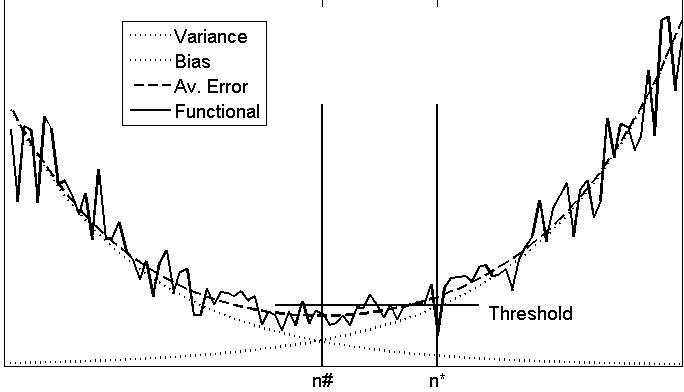
Figure 1: Idea of Proof

Let us consider the case $\chi(\cdot)=1$. At a first heuristic level the quasi-optimality criterion is plausible because by the geometric decay and growth in Assumption 2.1:

$$\tilde{\operatorname{{\mathbb{E}}}}[\lVert\hat{x}^{(n)}-\hat{x}^{(n+1)}\rVert^{2}]=(s(n+1)-s(n))+(b(n)-b(n+1))\asymp s(n)+b(n)=R_{2}(\hat{x}^{(n)})^{2}.$$

Hence, minimizing the criterion is related to minimizing the average case risk. Note, however, that a careful analysis is needed since the criterion is random and not at all independent of the estimator.

More generally, Definition 2.5 can be understood as a search for the intersection point $n^{\#}$ of the decreasing function $b(\cdot)$ and the increasing function $s(\cdot)$, where the minimal risk (with respect to $n$) is attained up to some constant factor, see Figure 1 and Lemma 3.2 below. Usually, comparably much is known about the variance part $s(\cdot)$ and not so much about the bias part $b(\cdot)$.

Let us briefly explain in words why the data-driven choice $n^{\ast}$ will be close to the intersection point $n^{\#}$ and therefore the resulting error in estimating $x$ does not change in order. As we face a symmetric situation (by exchanging the role of $s(\cdot)$ and $b(\cdot)$), we consider $n^{\ast}$ on the right side of $n^{\#}$ ($n^{\ast}>n^{\#}$).

In expectation (the situation depicted in Figure 1) the error curves meet at the oracle value $n^{\#}$. Here, though, we need to compute the probability that another point $n^{*}$ yields the minimal point for $\lVert\hat{x}^{(n+1)}-\hat{x}^{(n)}\rVert$.

To bound this probability, we introduce a threshold; the probability that $\lVert\hat{x}^{(n^{\#}+1)}-\hat{x}^{(n^{\#})}\rVert>\text{threshold}(n^{*})$ or $\lVert\hat{x}^{(n^{*}+1)}-\hat{x}^{(n^{*})}\rVert<\text{threshold}(n^{*})$ is larger than the desired probability for $\lVert\hat{x}^{(n^{\#}+1)}-\hat{x}^{(n^{\#})}\rVert>\lVert\hat{x}^{(n^{*}+1)}-\hat{x}^{(n^{*})}\rVert$ but much easier computable.

Furthermore, we completely ignore the fact we can just have one minimum, we replace $\tilde{\operatorname{{\mathbb{E}}}}[\lVert x-\hat{x}^{(n)}\rVert^{2}]$ by the sum of all positions where $n^{*}$ beats $n^{\#}$ weighted by the probability of their occurrence. Even for this very rough estimation this sum is still bounded from above by the order of the oracle. The formal mathematical statements are formulated along these lines in the next section.

3 The mathematical analysis

In this section we first determine a rate-optimal estimator for different moment-type losses, based on the (unrealistic) knowledge of the index $n^{\#}$ where the curves $b(\cdot)$ and $s(\cdot)$ intersect. Then we show that this rate does not deteriorate when we take the estimator with the data-driven index $n^{\ast}$, based on the quasi-optimality criterion of Definition 2.5. For the sake of readability all proofs are deferred to Section 6.

3.1 Risk for different moments

We denote the normalized Bayes risk for the moments of order $\alpha>0$ by

$$R_{\alpha}(\hat{x}^{(n)}):=\operatorname{{\mathbb{E}}}[\lVert\hat{x}^{(n)}-x\rVert^{\alpha}]^{1/\alpha},$$

consistent with the definition of $R_{2}(\hat{x}^{(n)})$. Note the order $R_{\alpha}(\hat{x}^{(n)})\leq R_{\beta}(\hat{x}^{(n)})$ for $\alpha\leq\beta$.

Definition 3.1.

Let $n^{\#}$ be the index where $s(n^{\#}+1)>b(n^{\#}+1)$ and $s(n^{\#})\leq b(n^{\#})$.

Note that $n^{\#}$ is uniquely defined by the monotonicity properties of $s(\cdot)$ and $b(\cdot)$. Interestingly, for $n^{\#}$ the risk is up to a multiplicative factor minimal, even under different moments:

Lemma 3.2.

Denote by $\Gamma$ the Gamma function and by $\zeta$ a standard normal random variable. With

$$K_{\alpha}:=\sqrt{2C_{b}}\,(4\Gamma(\tfrac{\alpha}{2}+1))^{1/\alpha}e^{-\operatorname{{\mathbb{E}}}[\log(\lvert\zeta\rvert)]}$$

the following bounds hold for all $\alpha>0$:

$$\forall n\in\operatorname{{\mathds{N}}}:\;R_{\alpha}(\hat{x}^{(n)}) \geq e^{\operatorname{{\mathbb{E}}}[\log(\lvert\zeta\rvert)]}R_{2}(\hat{x}^{(n)}),$$

$$\forall n\in\operatorname{{\mathds{N}}}:\;R_{\alpha}(\hat{x}^{(n)}) \leq(4\Gamma(\tfrac{\alpha}{2}+1))^{1/\alpha}R_{2}(\hat{x}^{(n)}),$$

$$\min_{n}R_{\alpha}(\hat{x}^{(n)}) \leq R_{\alpha}(\hat{x}^{(n^{\#})})\leq K_{\alpha}\min_{n}R_{\alpha}(\hat{x}^{(n)}).$$

We conclude from the last property that the risk (the expectation of the error) at the intersection point of $s(\cdot)$ and $b(\cdot)$ is bounded by a constant multiple of the minimal possible risk. The quasi-optimality criterion aims at recovering this index $n^{\#}$.

3.2 Main result

The first proposition quantifies the probability $\tilde{\operatorname{{\mathbb{P}}}}(n^{\ast}=n)$.

Proposition 3.3.

Grant Assumptions 2.1 and 2.3. Then

$$\tilde{\operatorname{{\mathbb{P}}}}(n^{\ast}=n)\leq(\sqrt{2}+(2er(n))^{r(n)/2})(\rho(n)\log(\rho(n)^{-1}))^{r(n)/2},$$

where

$$r(n):=\frac{\lvert\chi(n)\left((s(n+1)-s(n))+(b(n)-b(n+1))\right)\rvert}{\max_{\ell(n)<k\leq\ell(n+1)}(\sigma(k)^{2}+\gamma(k)^{2})}$$

and

$$\rho(n):=\begin{cases}\frac{C_{b}C_{s}-1}{c_{s}-1}(c_{s}C_{\chi}^{-1})^{-\lvert n-n^{\#}\rvert},&\text{for }n\geq n^{\#},\\ \frac{C_{b}C_{s}-1}{c_{b}-1}(c_{b}c_{\chi})^{-\lvert n-n^{\#}\rvert},&\text{for }n<n^{\#}.\end{cases}$$

Since $\rho(n)$ decays exponentially fast, this result yields a rapid decay for the probability that the minimal value for the quasi-optimality criterion is obtained away from the index $n^{\#}$. The slope of the exponential is largely depending on the subsampling function used, which will be investigated further in the upcoming example. We are now prepared to state and prove our main theorem.

Theorem 3.4.

Grant Assumptions 2.1 and 2.3 and set $r:=\inf_{n}r(n)$. Assume that $\alpha>0$ satisfies

$$\alpha<r\min\Big{(}\frac{\log(c_{b}c_{\chi})}{\log(C_{b})},\frac{\log(c_{s}/C_{\chi})}{\log(C_{s})}\Big{)}.$$

Then our estimator is almost surely well defined, i.e. the minimum in Definition 2.5 for $n^{\ast}$ is indeed attained, and it satisfies the oracle-type inequality

$$R_{\alpha}(\hat{x}^{(n^{\ast})})\leq K\min_{n}R_{\alpha}(\hat{x}^{(n)})$$

with a constant $K=K(c_{s},c_{b},C_{s},C_{b},c_{\chi},C_{\chi},r,\alpha)>0$.

Remark 3.5.

A closer look at the proof of Proposition 3.3 reveals that for this result only the boundedness and the decay behaviour of the Gaussian density was used. Hence, a similar result will hold for more general noise densities with exponential decay.

This oracle-type result, see e.g. Wasserman:2006 for a general discussion, is actually better than the classical statement obtained in inverse problems. There the results are given in the form [Engl/Hanke/Neubauer:1996]

$$\|x-\hat{x}^{(n^{\ast})}\|\leq c\delta^{\tau},$$

where $\tau$ is dependent on the type of noise and the source conditions. When $x$ or the noise have “accidentally” better properties than expected we still have this bound although $\min_{n}\|x-\hat{x}^{(n)}\|\ll c\delta^{\tau}$ for $\delta<\delta_{0}$.

In our case of an oracle inequality this cannot happen because we always compare with the best possible (“oracle”) solution. So we still have the theoretical upper bound in the form $c\delta^{\tau}$ but can additionally claim, that (in average) we are very close to the best possible solution, even if it is much better than any specific rate derived.

Although the mathematical result depends on a number of constants, it is important to note that the existence of these constants is required to derive the mathematical result, their actual values are not at all used for the quasi-optimality criterion.

It is interesting to note that though we face a stochastic noise we do not lose a logarithmic factor in the data-driven method as is sometimes the case for other parameter choice methods [Cohen/Hoffmann/Reiss:2004, Bauer/Pereverzev:2005].

The general picture is that our data-driven choice $n^{\ast}$ of the cut-off value yields an optimal risk bound up to constants whenever the moments taken are not so large. In order to achieve higher moments, we need to choose a subsampling function $\ell(n)$ that makes $r$ large enough. In any case, we have $r\geq 1$ by definition.

Example 3.6.

For the standard case of quadratic risk we need $\alpha=2$. For very tight exponential bounds $C_{s}\approx c_{s}$, $C_{b}\approx c_{b}$ and $\chi(\cdot)=1$ it suffices to have $r>2$. Now we can reconsider Example 2.2, where

$$a(n)\approx\frac{\delta^{2}\ell(0)^{2\nu+1}}{2\nu+1}(h^{2\nu+1})^{n}(h^{2\nu+1}-1)+\frac{\ell(0)^{-(2\mu-1)}}{2\mu-1}(h^{-2\mu+1})^{n+1}(h^{2\mu-1}-1)$$

Hence we have

$$r(n)\approx \min\left\{\frac{\frac{\delta^{2}\ell(0)^{2\nu+1}}{2\nu+1}(h^{2\nu+1})^{n}(h^{2\nu+1}-1)}{\delta^{2}(\ell(0)h^{n+1})^{2\nu}},\frac{\frac{\ell(0)^{-(2\mu-1)}}{2\mu-1}(h^{-2\mu+1})^{n+1}(h^{2\mu-1}-1)}{(\ell(0)h^{n})^{-2\mu}}\right\}$$

$$= \ell(0)\min\left\{\frac{1}{2\nu+1}h^{n-2\nu}(h^{2\nu+1}-1),\frac{1}{2\mu-1}h^{n-2\mu+1}(h^{2\mu-1}-1)\right\}$$

and so in the worst case

$$2<r\leq r(1)\approx\ell(0)h(h-1)=\ell(2)-\ell(1).$$

Thus the first (and smallest) distance $\ell(2)-\ell(1)$ needs to be at least $3$ in this case. This finding corresponds very well with numerical experience.

4 Application

In Bauer:2007 the quasi-optimality, Lepski balancing and hardened balancing principles have been compared numerically. The findings are that both, for a large scale stochastic experiment inverting ill-conditioned matrices and for a more realistic experiment determining the field of gravity from satellite data, quasi-optimality and hardened balancing perform quite well and stably, in particular better than the Lepski balancing principle.

The advantage of quasi-optimality is that it can cope with a rather unknown structure of the noise. Therefore we will present in the sequel numerical experiments for an inverse problem arising in option pricing where noise enters from various sources and its level is not easy to estimate.

The calibration of financial models based on option prices has attracted increasing attention recently due to its practical importance and mathematical challenges, see e.g. Crepey:2003 and Egger/Hein/Hofmann:2006 and the references therein for the case of a generalized Black-Scholes model and Chapter 13 in Cont/Tankov:2004 for jump models as considered here.

4.1 The calibration problem

We consider the problem of calibrating an exponential Lévy model based on market prices of European options and closely follow Belomestny/Reiss:2006. We briefly describe the problem, but refer to Cont/Tankov:2004 for a thorough introduction. It is assumed that we observe prices $C(K_{j})$ of European call options with different strike prices $K_{j}$, $j=1,\ldots,n$, and same time $T>0$ to maturity and that the underlying stock price follows an exponential Lévy process

$$S_{t}=S_{0}e^{L_{t}}\text{ with a L\'{e}vy process $(L_{t})$.}$$

Here, the Lévy process is restricted to be a superposition of a Brownian motion of volatility $\sigma^{2}>0$, a linear drift of slope $\gamma\in\operatorname{{\mathds{R}}}$ and a compound Poisson jump process of intensity $\lambda>0$ with jump density $\nu:\operatorname{{\mathds{R}}}\to\operatorname{{\mathds{R}}}^{+}$. The goal is to estimate these model parameters, in particular the jump density, which because of only finitely many observations and the presence of bid-ask spreads is a typical inverse problem with noisy observations in quantitative finance. The knowledge of these parameters permits to get a clear picture of the expectations at the market concerning future jumps in the stock price, which is essential for well-founded risk management and pricing of path-dependent options.

We transform the strike prices $(K_{j})$ to the so called log-forward moneyness $(x_{j})$ and the call option prices $C(K_{j})$ to a better behaved generalized option price function ${\cal O}(x_{j})$ and we introduce the weighted jump density $\mu(x)=e^{x}\nu(x)$. Then the forward formula, expressing option prices in terms of the model parameters, is given in the spectral domain by ($\cal F$ denotes the Fourier transform)

$${\cal FO}(v)=\frac{1-\exp(T(-\sigma^{2}(v-i)^{2}/2+i\gamma(v-i)+{\cal F}\mu(v)-\lambda))}{v(v-i)},\quad v\in\operatorname{{\mathds{R}}},$$

cf. Equation (2.7) in Belomestny/Reiss:2006. Our observations are modeled as

$$O_{j}={\cal O}(x_{j})+\varepsilon_{j},\quad j=1,\ldots,n,$$

with i.i.d. and centered noise variables $(\varepsilon_{j})$. For the sake of an easier presentation here, we assume that the real parameters $(\sigma^{2},\gamma,\lambda)$ are known such that the backward formula, expressing the transformed jump density in terms of the option prices, is given by

$${\cal F}\mu(v)=T^{-1}\log(1-v(v-i){\cal FO}(v))+\sigma^{2}(v-i)^{2}/2-i\gamma(v-i)+\lambda,\quad v\in\operatorname{{\mathds{R}}}.$$

We construct an empirical version $\tilde{\cal O}$ from the observations $(O_{j})$ (e.g. by linear interpolation) and obtain by substitution in this formula an empirical version ${\cal F}\tilde{\mu}(v)$ of ${\cal F}\mu(v)$, which satisfies for small noise levels

$$\lvert{\cal F}(\tilde{\mu}-\mu)(v)\rvert=T^{-1}{\Bigl{\lvert}\log\Big{(}\frac{1-v(v-i){\cal F\tilde{O}}(v)}{1-v(v-i){\cal FO}(v)}\Big{)}\Bigr{\rvert}}\approx T^{-1}{\Bigl{\lvert}\frac{v(v-i){\cal F(\tilde{O}-O)}(v)}{1-v(v-i){\cal FO}(v)}\Bigr{\rvert}}.$$

This first order analysis already reveals the ill-posedness of the calibration problem: the higher the frequency $\lvert v\rvert$, the more the error ${\cal F(\tilde{O}-O)}(v)$ in the observation domain is amplified by the factor $v(v-i)$ as well as by the denominator which tends to zero for $\lvert v\rvert\to\infty$. The nonlinearity is reflected by a noise level which depends on the unknown true value ${\cal FO}(v)$. A natural approach is to cut-off high frequencies and to consider for $U>0$ the estimators

$$\widehat{\mu}_{U}(x)={\cal F}^{-1}({\cal F}\tilde{\mu}{\bf 1}_{[-U,U]})(x),\quad x\in\operatorname{{\mathds{R}}}.$$

Let us write abstractly

$${\cal F}\tilde{\mu}(v)={\cal F}\mu(v)+\sigma(v)\xi(v),\quad v\in\operatorname{{\mathds{R}}},$$

with $\sigma(v)$ denoting the noise level and $\xi(v)$ denoting the normalized noise variable, that is the difference between empirical and true value divided by its standard deviation, at frequency $v$. Now we see the analogy with the sequence space model (2) analyzed before. In fact, the only difference is the continuity of the spectral parameter $v$ instead of $k\in\operatorname{{\mathds{N}}}$ and the additional difficulty is the much more complicated noise structure. Nevertheless, the estimators $\widehat{\mu}_{U}$ are provably rate-optimal for the right choice of the cut-off frequency $U$ (the problem is severely ill-posed in general). In simulations the standard data-driven choices of $U$ (e.g. Lepski’s method, cross validation) had a poor performance compared to the oracle choice, mostly because of a very badly known noise structure. This is exactly why the quasi-optimality criterion is of interest here.

4.2 Experimental Setup

In total we performed 1000 independent experiments. Each of them was set up as follows (notation as in Belomestny/Reiss:2006 where more details can be found):

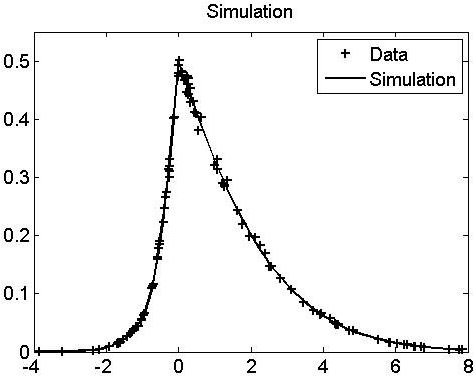
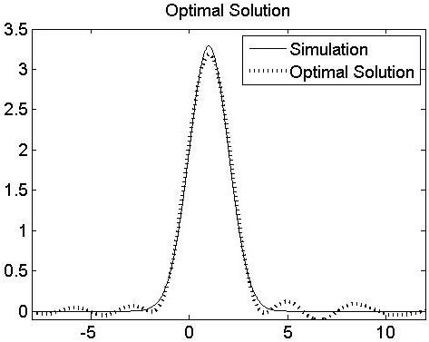
Figure 2: left: Data, right: optimal solution

• $100$ design points $(x_{i})$ were chosen at random, $50$ according to a standard normal, $50$ according to a uniform distribution on $[-4,8]$.

• Corresponding observations $(O_{i})$ are generated by calculating the exact value and adding standard normal noise of $3\%$ relative noise level, i.e. $O_{i}={\cal O}(x_{i})(1+0.03e_{i})$ with $e_{i}\stackrel{{\scriptstyle\text{iid}}}{{\sim}}\mathcal{N}(0,1)$. The other characteristics are chosen as follows (corresponding to the so-called Merton model): volatility $\sigma=0.1$, jumps are standard normal with intensity $\lambda=5$ (the jump density $\nu$ in Figure 2 (right)), maturity $T=0.25$. The value of $\gamma$ is obtained by imposing a martingale condition. In Figure 2 (left) the true option price function ${\cal O}(\cdot)$ is shown together with the observations as a function of $x$. Abstractly, one can show that in this setting both, the bias and the variance term have exponential decay respectively growth in $U$.

• In total $60$ cut-off frequencies $(U_{n})$ were chosen with step-width $0.8$, i.e. $U_{n}=0.8n$, $n=1,\ldots,60$.

4.3 Parameter choice methods

We will compare three different parameter choice methods. The quasi-optimality and the Hardened Balancing Principle are treated in this article and Lepski’s method serves as a widely used benchmark.

Quasi-Optimality.

We use exactly as in Definition 2.5 with $\chi(\cdot)=1$

$$n_{qo}:=\operatorname*{argmin}_{n}\{\|\hat{x}^{(n+1)}-\hat{x}^{(n)}\|\}.$$

Lepski-type method.

Define

$$f(n):=\max_{n<m\leq N}\left\{4^{-1}\|\hat{x}^{(m)}-\hat{x}^{(n)}\|/s(m)\right\},\quad n_{Lepski}:=\operatorname*{argmin}_{n}\{\forall m\geq n:\>f(m)\leq\kappa\}.$$

For the choice of $\kappa$ one should theoretically use a quantity depending on the noise level and larger than $1$. In practice, however, it is observed that $\kappa\in[0.25,0.75]$ gives superior results and works in more or less any situation. Here we choose $\kappa=0.75$.

Hardened Balancing Principle.

We reuse the computed quantity $f(n)$ defined above and choose as regularization parameter

$$n_{HBP}:=\operatorname*{argmin}_{n}\{f(n)\sqrt{s(n)}\}$$

Due to the definition of $f$ it can be seen as a stabilized version of Definition 2.5 with $\chi(n)={s(n)}^{-1/2}$. This stabilization mainly counters the effects of a subsampling with inappropriately small spacing between the cut-off points.

Implementation details.

There are certain fine points in the implementation, which are not crucial, but yield slightly superior results. The important point for the methods proposed here is the validity of Assumption 2.1. Therefore we estimated $s(\cdot)$ out of $10$ independent data sets (each of them constructed as given above, i.e. each of them with different design points and random error) and removed the cut-off parameters $n\in\{17,27,36,44,46,48\}$ which seem to violate the assumption empirically.

The Lepski balancing principle and Hardened Balancing show undesirable properties when $s(\max)/s(n)<2$. Therefore we restricted the region of admissible regularization parameters further to $n\in\{1,\ldots 43\}\setminus\{17,27,36\}$. The remaining cut-off points were still used to calculate the values $f(n)$.

4.4 Experiment

In Figure 3 the distribution of the efficiencies is displayed, i.e. the ratio of errors between the unsupervised solution selected by one of the methods and the optimal one, i.e.

$$\operatorname{efficiency}(x,y,n_{chosen}):=\|x^{(n_{chosen})}-x\|/\min_{n}\|x^{(n)}-x\|.$$

Note that the ratio cannot be smaller than $1$. Remark further that it is much harder to obtain a low value for $\mathbb{E}\operatorname{efficiency}(x,y,n_{chosen})$ compared to an oracle criterion of the form $\mathbb{E}\|x^{(n_{chosen})}-x\|/\min_{n}\mathbb{E}\|x^{(n)}-x\|$ because already one much better estimator in the denominator can spoil the results in our case. The bar plot of Figure 3 bins the solutions according to their efficiency. The bins are taken on a double exponential scale, ratios larger than 64 were considered as huge.

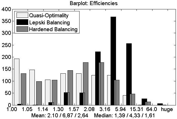
Figure 3: Efficiencies

As we can see, quasi-optimality and hardened balancing, as defined here, are superior to the Lepski-balancing principle, which suffers from a considerable number of bad results. Although in this situation the hardened balancing principle performs slightly worse, it has a particular advantage. Generally, it is relatively insensitive towards a bad choice of the subsampling whereas already one badly chosen distance in the subsampling could bring quasi-optimality out of track. Yet, it should be recalled that it relies significantly on an estimate of the stochastic noise level $s(\cdot)$, obtained from additional data sets.

5 Perspectives

Numerical experiments indicate that the results can be carried over to other regularization methods like Tikhonov regularization. Unfortunately, the correlation structure induced by Tikhonov regularization makes an analysis in comparison to the spectral cut-off regularization much more demanding and remains a topic of future research.

Interestingly, a way to improve the numerical results for spectral cut-off even further is to use a two-step procedure, where first a regularization parameter is obtained from a very coarse subsampling and then the region around the chosen regularization parameter is reconsidered with a finer subsampling. These types of procedures work provably well for change point detection problems (e.g. Korostelev:1987), a setting, which is to some extent related with our search for the intersection point of $b(\cdot)$ and $s(\cdot)$.

6 Proofs

In order to evaluate the probabilities of staying above or below the threshold, we will make use of the following technical result.

Lemma 6.1.

Let $Z=\sum_{k=1}^{\infty}\alpha_{k}^{2}\zeta_{k}^{2}$ with $\sum_{k=1}^{\infty}\alpha_{k}^{2}=1$ and $\zeta_{k}\sim N(0,1)$ iid. Then

$$\forall\,z\in(0,1):\;\operatorname{{\mathbb{P}}}(Z\leq z)\leq\exp\Big{(}\frac{1-z+\log(z)}{2\max_{k}\alpha_{k}^{2}}\Big{)},\qquad\forall\,z>0:\;\operatorname{{\mathbb{P}}}(Z\geq z)\leq\sqrt{2}e^{-z/4}.$$

Proof.

For all $\lambda>0$ and $z\in(0,1)$ we have

$$\operatorname{{\mathbb{P}}}(Z\leq z) =\operatorname{{\mathbb{P}}}\Big{(}\exp\Big{(}-\lambda\Big{(}\sum_{k=1}^{\infty}\alpha_{k}^{2}\zeta_{k}^{2}\Big{)}\Big{)}\geq e^{-\lambda z}\Big{)}$$

$$\leq e^{\lambda z}\prod_{k=1}^{\infty}\operatorname{{\mathbb{E}}}[\exp(-\lambda\alpha_{k}^{2}\zeta_{k}^{2})]$$

$$=e^{\lambda z}\prod_{k=1}^{\infty}(1+2\lambda\alpha_{k}^{2})^{-1/2}.$$

Due to $(1+2x)^{-1/2}\leq\exp(-\frac{\log(1+\varepsilon)}{\varepsilon}x)$ for $x\in[1,1+\varepsilon]$, $\varepsilon>0$, we deduce for $\lambda=\varepsilon(2\max_{k}\alpha_{k}^{2})^{-1}$ and $\varepsilon=z^{-1}-1$:

$$\operatorname{{\mathbb{P}}}(Z\leq z)\leq\exp\Big{(}\frac{\varepsilon}{2\max_{k}\alpha_{k}^{2}}\Big{(}z-\frac{\log(1+\varepsilon)}{\varepsilon}\Big{)}\Big{)}=\exp\Big{(}\frac{1-z+\log(z)}{2\max_{k}\alpha_{k}^{2}}\Big{)}.$$

By Jensen’s inequality we obtain for $z>0$

$$\operatorname{{\mathbb{P}}}(Z\geq z)\leq e^{-z/4}\operatorname{{\mathbb{E}}}\Big{[}\exp\Big{(}\sum_{k=1}^{\infty}\alpha_{k}^{2}\zeta_{k}^{2}/4\Big{)}\Big{]}\leq e^{-z/4}\operatorname{{\mathbb{E}}}[\exp(\zeta^{2}/4)]=\sqrt{2}e^{-z/4}.$$ (3)

∎

of Lemma 3.2.

For each $n\geq 1$ and $\alpha>0$ we derive from the concavity of the log-function and Jensen’s inequality

$$R_{\alpha}(\hat{x}^{(n)})^{2}=\tilde{\operatorname{{\mathbb{E}}}}[\lVert\hat{x}^{(n)}-x\rVert^{\alpha}]^{2/\alpha}$$

$$\geq\exp\big{(}\tilde{\operatorname{{\mathbb{E}}}}[\log(\lVert\hat{x}^{(n)}-x\rVert^{2})]\big{)}$$

$$=\exp\Big{(}\tilde{\operatorname{{\mathbb{E}}}}\Big{[}\log\Big{(}\sum_{k=1}^{\ell(n)}\tfrac{\sigma(k)^{2}\xi_{k}^{2}}{s(n)+b(n)}+\sum_{k=\ell(n)+1}^{\infty}\tfrac{x_{k}^{2}}{s(n)+b(n)}\Big{)}\Big{]}+\log(s(n)+b(n))\Big{)}$$

$$\geq\exp\Big{(}\sum_{k=1}^{\ell(n)}\tfrac{\sigma(k)^{2}}{s(n)+b(n)}\tilde{\operatorname{{\mathbb{E}}}}[\log(\xi_{k}^{2})]+\sum_{k=\ell(n)+1}^{\infty}\tfrac{\gamma(k)^{2}}{s(n)+b(n)}\tilde{\operatorname{{\mathbb{E}}}}[\log(x_{k}^{2}/\gamma(k)^{2})]\Big{)}(s(n)+b(n))$$

$$=(s(n)+b(n))e^{\operatorname{{\mathbb{E}}}[\log(\zeta^{2})]}=e^{\operatorname{{\mathbb{E}}}[\log(\zeta^{2})]}R_{2}(\hat{x}^{(n)})^{2},$$

which gives the first inequality. For the second, we use $w^{\alpha/2}/\Gamma(\frac{\alpha}{2}+1)\leq e^{w}$ for $w\geq 0$, Lemma 6.1 and $(1-w)^{-1/2}\leq 2^{w}$ for $w\in(0,1/2]$ to obtain for any $\alpha>0$ and $\lambda\in(0,\min(\gamma(\ell(n)+1)^{-2},\sigma(\ell(n))^{-2})/4)$:

$$\tilde{\operatorname{{\mathbb{E}}}}[\lVert\hat{x}^{(n)}-x\rVert^{\alpha}] =\Gamma(\tfrac{\alpha}{2}+1)\lambda^{-\alpha/2}\tilde{\operatorname{{\mathbb{E}}}}[\lambda^{\alpha/2}\lVert\hat{x}^{(n)}-x\rVert^{\alpha}/\Gamma(\tfrac{\alpha}{2}+1)]$$

$$\leq\Gamma(\tfrac{\alpha}{2}+1)\lambda^{-\alpha/2}\tilde{\operatorname{{\mathbb{E}}}}[\exp(\lambda\lVert\hat{x}^{(n)}-x\rVert^{2})]$$

$$=\Gamma(\tfrac{\alpha}{2}+1)\lambda^{-\alpha/2}\prod_{k=1}^{\ell(n)}(1-2\lambda\sigma(k)^{2})^{-1/2}\prod_{k=\ell(n)+1}^{\infty}(1-2\lambda\gamma(k)^{2})^{-1/2}$$

$$\leq\Gamma(\tfrac{\alpha}{2}+1)\lambda^{-\alpha/2}\exp(2\log(2)\lambda(s(n)+b(n))).$$

The choice $\lambda=(s(n)+b(n))^{-1}$ fulfills the above requirement and thus yields

$$R_{\alpha}(\hat{x}^{(n)})=\tilde{\operatorname{{\mathbb{E}}}}[\lVert\hat{x}^{(n)}-x\rVert^{\alpha}]^{1/\alpha}\leq(4\Gamma(\tfrac{\alpha}{2}+1))^{1/\alpha}R_{2}(\hat{x}^{(n)}).$$

The last inequality follows from the two others together with the fact that Assumption 2.1 implies

$$\min_{n}R_{2}(\hat{x}^{(n)})^{2}\geq\min(b(n^{\#}),s(n^{\#}+1))\geq\tfrac{C_{b}^{-1}}{2}R_{2}(\hat{x}^{(n^{\#})})^{2}.$$

∎

of Proposition 3.3.

Let us first introduce the following quantities:

$$a(n) :=\sqrt{\chi(n)}\sqrt{(s(n+1)-s(n))+(b(n)-b(n+1))},$$

$$D(n) :=\chi(n)\lVert\hat{x}^{(n+1)}-\hat{x}^{(n)}\rVert^{2},$$

$$Z(n) :=\sqrt{D(n)}/a(n).$$

We shall only consider $n>n^{\#}$ because the case $n<n^{\#}$ is symmetric (exchanging $s$ and $b$) and the case $n=n^{\#}$ is trivial. For $m:=n-n^{\#}\geq 1$ we find by Assumptions 2.1 and 2.3

$$\frac{a(n^{\#})^{2}}{a(n^{\#}+m)^{2}} \leq\frac{\chi(n^{\#})}{\chi(n^{\#}+m)}\frac{(C_{s}-1)s(n^{\#})+(C_{b}-1)b(n^{\#}+1)}{(c_{s}-1)s(n^{\#}+m)}$$

$$\leq{C_{\chi}}^{m}\;\frac{(C_{s}-1)s(n^{\#})+(C_{b}-1)s(n^{\#}+1)}{(c_{s}-1)c_{s}^{m}s(n^{\#})}$$

$$\leq\frac{C_{b}C_{s}-1}{c_{s}-1}\left(\frac{c_{s}}{{C_{\chi}}}\right)^{-m}=\rho(n).$$

Using Lemma 6.1, we infer for any $K>0$

$$\tilde{\operatorname{{\mathbb{P}}}}(n^{\ast}=n) \leq\tilde{\operatorname{{\mathbb{P}}}}(D(n)\leq D(n^{\#}))$$

$$\leq\tilde{\operatorname{{\mathbb{P}}}}(Z(n)^{2}\leq\rho(n)Z(n^{\#})^{2})$$

$$\leq\tilde{\operatorname{{\mathbb{P}}}}(Z(n)^{2}\leq K\rho(n)\log(\rho(n)^{-1}))+\tilde{\operatorname{{\mathbb{P}}}}(Z(n^{\#})^{2}\geq K\log(\rho(n)^{-1}))$$

$$\leq\exp\left(\frac{1-K\rho(n)\log(\rho(n)^{-1})+\log(K\rho(n)\log(\rho(n)^{-1}))}{2\max_{k}\frac{\sigma(k)^{2}+\gamma(k)^{2}}{a(n)}}\right)$$

$$\qquad+\sqrt{2}\exp(-K\log(\rho(n)^{-1})/4)$$

$$\leq(Ke\rho(n)\log(\rho(n)^{-1}))^{a(n)^{2}/2\max_{k}(\sigma(k)^{2}+\gamma(k)^{2})}+\sqrt{2}\rho(n)^{K/4}$$

$$=\sqrt{2}\rho(n)^{K/4}+(Ke\rho(n)\log(\rho(n)^{-1}))^{r(n)/2}.$$

The choice $K=2r(n)$ yields the result. ∎

of Theorem 3.4.

To prove that $n^{\ast}$ is well defined, we infer from the proof of Proposition 3.3 that for all $n>n^{\ast}$

$$\tilde{\operatorname{{\mathbb{P}}}}(D(n)\leq D(n^{\#}))\leq\sqrt{2}\rho(n)^{r(n)/2}+(2er(n)\rho(n)\log(\rho(n)^{-1}))^{r(n)/2}.$$

This exponential decay implies

$$\lim_{m\to\infty}\tilde{\operatorname{{\mathbb{P}}}}(\exists n\geq m:\>D(n)\leq D(n^{\#}))\leq\lim_{m\to\infty}\sum_{n=m}^{\infty}\tilde{\operatorname{{\mathbb{P}}}}(D(n)\leq D(n^{\#}))=0,$$

which means that the probability that the criterion $D(\cdot)$ is larger for some $n\geq m$ than at $n^{\#}$ tends to zero as $m\to\infty$, hence $n^{\ast}=\operatorname*{argmin}_{n}D(n)$ is well defined with probability one.

For the main assertion we use Hölder’s inequality with $p^{-1}+q^{-1}=1$, Lemma 3.2 and Assumption 2.1 for any $\alpha>0$ to obtain:

$$\tilde{\operatorname{{\mathbb{E}}}}[\lVert\hat{x}^{(n^{\ast})}-x\rVert^{\alpha}]$$

$$=\sum_{m=-n^{\#}+1}^{\infty}\tilde{\operatorname{{\mathbb{E}}}}[\lVert\hat{x}^{(n^{\#}+m)}-x\rVert^{\alpha}{\bf 1}_{\{n^{\ast}=n^{\#}+m\}}]$$

$$\leq\sum_{m=-n^{\#}+1}^{\infty}\tilde{\operatorname{{\mathbb{E}}}}[\lVert\hat{x}^{(n^{\#}+m)}-x\rVert^{\alpha p}]^{1/p}\tilde{\operatorname{{\mathbb{E}}}}[{\bf 1}_{\{n^{\ast}=n^{\#}+m\}}^{q}]^{1/q}$$

$$\leq\sum_{m=-n^{\#}+1}^{\infty}R_{\alpha p}(\hat{x}^{(n^{\#}+m)})^{\alpha}\tilde{\operatorname{{\mathbb{P}}}}(n^{\ast}=n^{\#}+m)^{1/q}$$

$$\leq(4\Gamma(\tfrac{\alpha p}{2}+1))^{1/p}\sum_{m=-n^{\#}+1}^{\infty}R_{2}(\hat{x}^{(n^{\#}+m)})^{\alpha}\tilde{\operatorname{{\mathbb{P}}}}(n^{\ast}=n^{\#}+m)^{1/q}$$

$$\leq(4\Gamma(\tfrac{\alpha p}{2}+1))^{1/p}\big{(}2s(n^{\#})\big{)}^{\alpha}\Big{(}\sum_{m=0}^{\infty}C_{s}^{\alpha m/2}\tilde{\operatorname{{\mathbb{P}}}}(n^{\ast}=n^{\#}+m)^{1/q}+\sum_{m=0}^{n^{\#}-1}C_{b}^{\alpha m/2}\tilde{\operatorname{{\mathbb{P}}}}(n^{\ast}=n^{\#}-m)^{1/q}\Big{)}.$$

We choose $q:=(\frac{\alpha}{2}+\frac{r}{2}\min(\frac{\log(c_{b}c_{\chi})}{\log(C_{b})},\frac{\log(c_{s}/C_{\chi})}{\log(C_{s})}))/\alpha>1$ and infer from Proposition 3.3

$$\sum_{m=1}^{\infty}C_{s}^{\alpha m/2}\tilde{\operatorname{{\mathbb{P}}}}(n^{\ast}=n^{\#}+m)^{1/q}$$

$$\leq(\sqrt{2}+(2er)^{r/2})^{1/q}\left(\frac{C_{b}C_{s}-1}{c_{s}-1}\log\left(\frac{c_{s}-1}{C_{b}C_{s}-1}\frac{c_{s}}{C_{\chi}}\right)\right)^{r/2q}\sum_{m=1}^{\infty}C_{s}^{\alpha m/2}\left(\frac{c_{s}}{C_{\chi}}\right)^{-rm/2q}m^{r/2q},$$

which is finite by the choice of $q$ and the restriction on $\alpha$. With a symmetric argument for $m\leq 0$ we conclude that $\tilde{\operatorname{{\mathbb{E}}}}[\lVert\hat{x}^{(n^{\ast})}-x\rVert^{\alpha}]$ is bounded by a multiple of $s(n^{\#})^{\alpha/2}$, which has the order of $R_{2}(\hat{x}^{(n^{\#})})^{\alpha}$. We eventually obtain with constants $K=K(c_{s},c_{b},C_{s},C_{b},r,\alpha)$, $K^{\prime}=K^{\prime}(c_{s},c_{b},C_{s},C_{b},r,\alpha)$ (note that $p$ and $q$ depend on $\alpha$ and the remaining constants):

$$R_{\alpha}(\hat{x}^{(n^{\ast})}) \leq K^{\prime}R_{2}(\hat{x}^{(n^{\#})})\leq K\min_{n\geq 1}R_{\alpha}(\hat{x}^{(n)}).$$

∎

References

- [1] \harvarditem[Bakushinskii]Bakushinskii1984Bakushinskii:1984 Bakushinskii, A. (1984): “Remarks on choosing a regularization parameter using the quasi-optimality and ratio criterion,” Comput. Maths. Math. Phys., 24(4), 181–182.
- [2] \harvarditem[Bauer]Bauer2007Bauer:2007 Bauer, F. (2007): “Some considerations concerning regularization and parameter choice algorithms,” Inverse Problems, 23, 837–858.
- [3] \harvarditem[Bauer and Pereverzev]Bauer and Pereverzev2005Bauer/Pereverzev:2005 Bauer, F., and S. Pereverzev (2005): “Regularization without preliminary knowledge of smoothness and error behavior,” European Journal of Applied Mathematics, 16(3), 303–317.
- [4] \harvarditem[Belomestny and Reiß]Belomestny and Reiß2006Belomestny/Reiss:2006 Belomestny, D., and M. Reiß (2006): “Spectral calibration of exponential Lévy models,” Finance Stoch., 10(4), 449–474.
- [5] \harvarditem[Cohen, Hoffmann, and Reiß]Cohen, Hoffmann, and Reiß2004Cohen/Hoffmann/Reiss:2004 Cohen, A., M. Hoffmann, and M. Reiß (2004): “Adaptive wavelet Galerkin methods for linear inverse problems,” SIAM Journal of Numerical Analysis, 42(4), 1479–1501.
- [6] \harvarditem[Cont and Tankov]Cont and Tankov2004Cont/Tankov:2004 Cont, R., and P. Tankov (2004): Financial Modelling with Jump Processes. Chapman & Hall/CRC Financial Mathematics Series. Boca Raton, FL: Chapman and Hall/CRC.
- [7] \harvarditem[Crépey]Crépey2003Crepey:2003 Crépey, S. (2003): “Calibration of the local volatility in a generalized Black–Scholes model using Tikhonov regularization.,” SIAM J. Math. Anal., 34(5), 1183–1206.
- [8] \harvarditem[Egger, Hein, and Hofmann]Egger, Hein, and Hofmann2006Egger/Hein/Hofmann:2006 Egger, H., T. Hein, and B. Hofmann (2006): “On decoupling of volatility smile and term structure in inverse option pricing.,” Inverse Probl., 22(4), 1247–1259.
- [9] \harvarditem[Engl, Hanke, and Neubauer]Engl, Hanke, and Neubauer1996Engl/Hanke/Neubauer:1996 Engl, H., M. Hanke, and A. Neubauer (1996): Regularization of Inverse Problems. Kluwer Academic Publisher, Dordrecht, Boston, London.
- [10] \harvarditem[Kaipio and Somersalo]Kaipio and Somersalo2005Kaipio/Somersalo:2005 Kaipio, J., and E. Somersalo (2005): Statistical and Computational Inverse Problems, vol. 160 of Applied Mathematical Sciences. Springer-Verlag, New York.
- [11] \harvarditem[Korostelev]Korostelev1987Korostelev:1987 Korostelev, A. (1987): “On minimax estimation of a discontinuous signal,” Theory Prob. Appl., 32(4), 727–730.
- [12] \harvarditem[Lepski]Lepski1990Lepskij:1990 Lepski, O. (1990): “On a problem of adaptive estimation in Gaussian white noise,” Theory of Probability and its Applications, 35(3), 454–466.
- [13] \harvarditem[Tikhonov and Arsenin]Tikhonov and Arsenin1977Tikhonov/Arsenin:1977 Tikhonov, A., and V. Arsenin (1977): Solutions of Ill-Posed Problems. Wiley, New York.
- [14] \harvarditem[Tikhonov, Glasko, and Kriksin]Tikhonov, Glasko, and Kriksin1979Tikhonov/Glasko/Kriksin:1979 Tikhonov, A., V. Glasko, and Y. Kriksin (1979): “On the question of quasi-optimal choice of a regularized approximation.,” Sov. Math. Dokl., 20, 1036–1040.
- [15] \harvarditem[Wahba]Wahba1977Wahba:1977 Wahba, G. (1977): “Practical approximate solutions to linear operator equations when the data are noisy,” SIAM Journal on Numerical Analysis, 14(4), 651–667.
- [16] \harvarditem[Wasserman]Wasserman2006Wasserman:2006 Wasserman, L. (2006): All of Nonparametric Statistics. Springer Texts in Statistics. New York, NY: Springer.
- [17]