The XMM-Newton Bright Serendipitous Survey

Abstract

Aims. We present the optical classification and redshift of 348 X-ray selected sources from the XMM-Newton Bright Serendipitous Survey (XBS) which contains a total of 400 objects (identification level = 87%). About 240 are new identifications. In particular, we discuss in detail the classification criteria adopted for the Active Galactic Nuclei population.

Methods. By means of systematic spectroscopic campaigns and through the literature search we have collected an optical spectrum for the large majority of the sources in the XBS survey and applied a well-defined classification “flow-chart”.

Results. We find that the AGN represent the most numerous population at the flux limit of the XBS survey ($\sim$10^-13 erg cm^-2 s^-1) constituting 80% of the XBS sources selected in the 0.5-4.5 keV energy band and 95% of the “hard” (4.5-7.5 keV) selected objects. Galactic sources populate significantly the 0.5-4.5 keV sample (17%) and only marginally (3%) the 4.5-7.5 keV sample. The remaining sources in both samples are clusters/groups of galaxies and normal galaxies (i.e. probably not powered by an AGN). Furthermore, the percentage of type 2 AGN (i.e. optically absorbed AGNs with A${}_{V}>2$mag) dramatically increases going from the 0.5-4.5 keV sample (f=N_AGN2/N_AGN=7%) to the 4.5-7.5 keV sample (f=32%). We finally propose two simple diagnostic plots that can be easily used to obtain the spectral classification for relatively low redshift AGNs even if the quality of the spectrum is not good.

1 Introduction

In the last few years XMM-Newton and Chandra telescopes have represented an excellent tool to survey the hard X-ray sky at all fluxes, from relatively bright (10^-13 erg cm^-2 s^-1, e.g. Della Ceca et al. 2004 and references therein), to medium (10^-13 erg cm^-2 s^-1-10^-14 erg cm^-2 s^-1, e.g. Barcons et al. 2007 and references therein) and deep (10^-14-10^-16 erg cm^-2 s^-1, Brandt & Hasinger 2005; Worsley et al. 2005 and references therein) fluxes. At the energies ($\sim$0.5-10 keV) covered by the instruments on board these two telescopes, Active Galactic Nuclei (AGN) can be efficiently selected and studied even when affected by large levels of absorption (up to N${}_{H}\sim$10²⁴ cm^-2, corresponding to an optical absorption of A${}_{V}\sim$500 mag). This important characteristic, combined with the good/excellent spatial and energy resolutions of the detectors, makes the ongoing surveys a fundamental tool for AGN studies. At the same time, these new surveys represent an observational challenge at wavelengths different from the X-ray ones: multiwavelength follow-ups of X-ray sources, particularly in the optical domain, are decisive to derive the distance and to understand the properties of the selected objects but they also require large fractions of dedicated observing time at different telescopes. Probably one of the most challenging and time-consuming efforts is the optical spectroscopic follow-up of the selected sources.

One of the primary goals of all these hard X-ray surveys is to explore the population of absorbed AGN and, to this end, an optical classification that can reliably separate between optically absorbed and non-absorbed objects is always required. Two important limits, however, affect the spectroscopic follow-ups of deep and, in part, medium surveys: first, the optical counterparts are often too faint to be spectroscopically observed even at the largest optical telescopes currently available; second, even when a spectrum can be obtained, its quality is not always good enough to provide the critical pieces of information that are required to assess a reliable optical classification. These two problems often limit the final scientific results that are based on the optical classification of medium/deep surveys.

On the contrary, bright surveys offer the important possibility of obtaining a reliable optical classification for virtually all (with some exceptions, as discussed in the next sections) the selected sources. The disadvantage of dealing with shallow/wide-angle samples is that the techniques to observe efficiently many sources at once, like Multi-objects or fibers-based methods, cannot be applied for the optical follow-up, given the low space-density of sources at bright X-ray fluxes. The only suitable method, the “standard” long-slit technique, requires many independent observing nights to achieve the completion of the optical follow-up.

In this paper we present and discuss in detail the optical classification process of the XMM-Newton Bright Serendipitous Survey (XBS, Della Ceca et al. 2004), which currently represents the widest (in terms of sky coverage) among the existing XMM-Newton or Chandra surveys for which a spectroscopic follow-up has been almost completed. The aim of the paper, in particular, is to provide not only a generic classification of the sources and their redshift but also a quantification, in the limits of the available data, of the corresponding threshold in terms of level of optical absorption.

The paper is organized as follows: in Section 2 we describe the XBS survey, in Section 3 we describe the process of identification of the optical counterpart, in Section 4 and Section 5 we respectively summarize our own spectroscopic campaigns carried out to collect the data as well as the data obtained from the literature. In Section 6 we shortly discuss the data reduction and analysis of the optical spectra and in Section 7 we give the details on the classification criteria adopted for the sources in the XBS survey. In Section 8 we propose two diagnostic plots that can be used to easily classify the sources into type 1 and type 2 AGN. The resulting catalogue is presented in Section 9 while in Section 10 we briefly discuss the optical breakdown and the redshift distribution of the sources. The conclusions are finally summarized in Section 11 . Throughout this paper H₀=65 km s^-1 Mpc^-1, $\Omega_{\Lambda}$=0.7 and $\Omega_{M}$ = 0.3 are assumed.

2 The XMM-Newton Bright Serendipitous Survey

The XMM-Newton Bright Serendipitous Survey (XBS survey, Della Ceca et al. 2004) is a wide-angle ($\sim$28 sq. deg) high Galactic latitude ($|b|>$20 $\deg$) survey based on the XMM-Newton archival data. It is composed of two samples both flux-limited ($\sim$7$\times$10^-14 erg cm^-2 s^-1) in two separate energy bands: the “soft” 0.5-4.5 keV band (the BSS sample) and the hard 4.5-7.5 keV band (the HBSS sample). A total of 237 (211 for the HBSS sample) independent fields have been used to select 400 sources, 389 belonging to the BSS sample and 67 to the HBSS sample (56 sources are in common). The details on the fields selection strategy, the sources selection criteria and the general properties of the 400 objects are discussed in Della Ceca et al. (2004).

One of the main goals of the survey is to provide a well-defined and statistically complete census of the AGN population with particular attention to the problem of obscuration. To this end, the possibility of comparing X-ray and optical spectra of good quality for all the sources present in the two complete samples offers a unique and fundamental tool to statistically study the effect of absorption in the AGN population in an unbiased way. Indeed, most of the X-ray sources of the XBS survey have been detected with enough counts to allow a reliable X-ray spectral analysis. At the same time, most of the sources have a relatively bright (R$<$22 mag, see next section) optical counterpart and they can be spectroscopically characterized using a 4-meters-class telescope.

To date, the spectroscopic identification level has reached 87% (87% and 97% considering the BSS and the HBSS samples separately). The results of the spectroscopic campaigns are discussed in the following sections.

3 Identification of the optical counterpart

Figure 1: Magnitude distribution of the XBS optical counterparts. Most (94%) of the magnitudes are in a red filter. Shaded histogram represents the sources without a spectral classification.

The identification of the optical counterparts of the XBS sources is relatively easy given the combination of the good positions of the XMM-Newton sources (90% error $\sim$4″, Della Ceca et al. 2004) and the brightness of the sources: X-ray sources with F${}_{X}>$10^-13 erg cm^-2 s^-1 are expected to have an optical counterpart brighter than 22 mag for X-ray-to-optical flux ratios below 20 (i.e. for the majority of type 1 AGN, galaxies and stars). Only the rare (but interesting) sources with extreme X-ray-to-optical flux ratios, like the distant type 2 QSOs (e.g. Severgnini et al. 2006), are expected to have magnitudes as faint as R$\sim$25. For this reason, for the large majority of the XBS sources we have been able to unambiguously pinpoint the optical counterpart using the existing optical surveys (i.e. the DSS I/II and the SDSS). In particular, we have found the optical counterpart of about 88% of the XBS sources on the DSS with a red magnitude (the APM red magnitude) brighter than $\sim$20.5. All but 6 of the remaining sources have been optically identified either through dedicated photometry or using the SDSS catalogue. The red magnitudes of these sources are relatively bright (R between 20.5 and 22.5) with one exception: an R=24.5 object (XBSJ021642.3-043553), that turned out to be a distant (z=1.985) type 2 QSO (Severgnini et al. 2006). For 6 objects we have not yet found the optical counterpart but only for two of these we have relatively deep images that have produced a faint lower limit on the R magnitude (R$>$22.8 and R$>$22.2 respectively). For the other 4 sources we only have the upper limit based on the DSS plates.

Figure 2: X-ray/optical positional offsets of the 348 XBS sources with a spectral classification. Open circles are stars and clusters of galaxies while filled points are the remaining sources (AGNs and “elusive AGN candidates”). The two circles represent the regions including 68% and 90% of the points

Figure 3: X-ray/optical positional offsets of the XBS sources in common with the 2XMM catalogue (343 in total). In this case the X-ray positions are taken from the 2XMM catalogue that has been produced with recent versions of the Standard Analysis System. Symbols and regions as in Fig. 2

In conclusion, we have found the most-likely optical counterpart in the large majority of the 400 XBS sources (all but 6 sources). The magnitude distribution of the counterparts is presented in Fig. 1. Since we have not carried out a systematic photometric follow-up of the XBS objects, we do not have an homogeneous set of magnitudes in a well defined filter. In Fig. 1 we have reported the magnitudes either from existing catalogues (e.g. APM, SDSS, NED, Simbad) or from our own observations. Most of them (94%) are in a red filter while the remaining 6% (all bright stars with mag$<$13) are in V or B filters.

In Fig. 2 we show the X-ray/optical positional offsets of the 348 XBS sources discussed in this paper (i.e. those with a spectral classification). All the identifications have offsets below $\sim$7$\arcsec$, with the majority ($\sim$90%) of sources having an offset below 3.8$\arcsec$. In Fig 2 we have distinguished the objects spectroscopically classified as stars and clusters of galaxies (indicated with open circles) from the rest of the sources (filled circles) since both stars and clusters may suffer from larger positional offsets due to the presence of proper motions (stars) or, in the case of clusters of galaxies, due to the intrinsic offset between the X-ray source (the intracluster gas) and the optical object (e.g. the cD galaxy). Indeed, the circle including 90% of stars and clusters is larger ($\sim$4.5$\arcsec$) than the circle computed using all the sources.

In the last years the XMM-Newton images have been reprocessed with improved versions of the SAS and the astrometry has been refined and corrected. We have thus recomputed the X-ray-optical offsets using the improved X-ray positions included in the preliminary version of the second XMM-Newton Serendipitous EPIC Source Catalogue (2XMM, Watson et al. 2007, in preparation, see also http://xmm.vilspa.esa.es/xsa/). In Fig. 3 we plot these newly computed offsets for the objects that are in common with the 2XMM catalogue. The improvement is evident, with 90% of the sources (excluding stars and clusters) having an offset below 2.1$\arcsec$. The sources with relatively large offsets (4-5$\arcsec$) are mostly stars and clusters. All but 2 extragalactic “non-clusters” objects have X-ray-to-optical offsets below 4″. By inspecting the X-ray images of the two extragalactic “non-clusters” objects with large offsets (XBSJ095054.5+393924, a type 1 QSO at z=1.299 and XBSJ225020.2-64290, a type 1 QSO at z=1.25) we have found strong indications that both objects are the result of a source blending which has “moved” the centroid of the X-ray position between two nearby objects. Interestingly, in one of these cases (XBSJ225020.2-642900) we have spectroscopically observed also the second (and fainter) nearby object and found a very similar spectrum of type 1 QSO at the same redshift (1.25). This could either be a real QSO pair or, alternatively, the result of gravitational lensing caused by a (not visible) galaxy.

In conclusion, excluding these two objects, for which the X-ray position is not accurate, all the XBS sources classified as extragalactic objects have an optical counterpart within 4″ using the improved X-ray positions and 90% have offsets within 2.1″.

3.1 Estimate of the number of spurious X-ray/optical associations

As discussed above, the optical counterparts found for the XBS sources have R magnitudes brighter than 22.5 (except for one object) with a large fraction (88%) of them having magnitudes brighter than 20.5 (i.e. they are visible on the DSS plates). Given the density of AGN at the magnitude limit of R=22.5 (e.g. Wolf et al. 2003), the probabilty of finding an AGN by chance within 4$\arcsec$ from an unrelated X-ray source is $\sim$5$\times$10^-4 which translates into an expected number of $\sim$0.2 spurious AGN identifications in the entire XBS survey. Therefore it is reasonable to consider all the objects optically classified as emission line AGN (or BL Lac objects) as the correct counterparts of the X-ray sources. Stars and galaxies, instead, may contaminate the identification process, given their higher sky density. In principle, a fraction of sources identified as stars or “normal” galaxies (or elusive AGN, see discussion in Sec. 7.5) could be spurious counterparts. Considering the density of stars and galaxies at the faintest magnitudes observed in the two classes of sources (R${}_{stars}\leq$18 and R${}_{galaxies}\leq$21) we expect about 12 stars and 4 galaxies falling by chance within 4$\arcsec$ from the 400 X-ray positions. This is clearly an upper limit given the adopted identification process: we have usually observed all the bright (i.e. visible on the DSS) objects falling within the circle of 4$\arcsec$ radius and, whenever an AGN is found we have considered it as the right counterpart (as described above the probability of finding an AGN by chance is very low in our survey) and discarted the others (either stars or galaxies). This strategy excludes the large majority of possible spurious galaxy or star identifications: only those stars or galaxies falling by chance close to an X-ray source whose real counterpart is weak (e.g weaker than the DSS limit) have the possibility of being considered the counterpart by mistake. Since the majority ($\sim$90%) of the real counterparts are expected to be brighter than the DSS limit, we conclude that only $\sim$1/10 of the 12 stars and 4 galaxies falling by chance in the error circle have the possibility of being considered as the counterpart. Therefore, the actual number of spurious stars and galaxies in the sample should be $\sim$1.2 and $\sim$0.4 respectively. In conclusion, we do not expect more than 1-2 mis-identifications in the entire XBS survey.

4 Optical spectroscopy

About 2/3 of the spectroscopic identifications (i.e. $\sim$240 objects) of the XBS survey come from dedicated spectroscopy carried out during 5 years (from 2001 to 2006) at several optical telescopes. Most of the identifications are obtained at the Italian Telescopio Nazionale Galileo (TNG, 51% of the identifications) and at the ESO 3.6m and NTT telescopes (37%). The remaining 12% has been collected from other telescopes like the 88” telescope of the University of Hawaii (UH) in Mauna Kea and the Calar Alto 2.2m telescope.

The instrumental configurations are summarized in Table 1. We have always adopted a long-slit configuration with low/medium dispersion (from 1.4 Å/pixel to 3.7 Å/pixel) and low/medium resolution (from $\sim$250 to 450) grisms to maximize the wavelength coverage. For the data reduction we have used the IRAF longslit package. The spectra have been wavelength calibrated using a reference spectrum and flux calibrated using photometric standard stars observed during the same night. Most of the observations were carried out during non-photometric conditions. Since the main goal of the observations was to secure a redshift and a spectral classification of the source we did not attempt to obtain an absolute flux calibration of the spectra.

Telescope/instrument/grism	slit width	dispersion	Observing nights
	(arcsec)	(Å/pixel)
TNG+DOLORES+LRB	1.5, 2	2.8	15-16/11/2001
UH88”+WFGS+green(400)	1.6	3.7	16-18/04/2002
ESO3.6m+EFOSC+Gr6	1.2	2.1	02-08/05/2002
TNG+DOLORES+LRB	1.5	2.8	23/06/2002
TNG+DOLORES+LRB	1.5	2.8	09-12/09/2002
ESO3.6m+EFOSC+Gr13	1.2, 1.5	2.8	30/09-02/10/2002
TNG+DOLORES+LRB	1.5	2.8	05-07/10/2002
CA2.2m+CAFOS+B200/R200	1.5	4.7/4.3	30/10-01/11/2002
TNG+DOLORES+LRB	1.5	2.8	25-27-28/12/2002
TNG+DOLORES+LRB	1.5	2.8	27-30/03/2003
NTT+EMMI+Gr3	1.0	1.4	02-03/05/2003
TNG+DOLORES+LRB	1.5	2.8	08/05/2003
TNG+DOLORES+LRB	1.5	2.8	27/09-01/10/2003
NTT+EMMI+Gr2	1.0, 1.5	1.7	04-06/01/2005
TNG+DOLORES+LRB	1.5	2.8	12-16/03/2005
NTT+EMMI+Gr2	1.5	1.7	07/10/2005
NTT+EMMI+Gr2	1.0, 1.5, 2.0	1.7	02-05/03/2006

Table 1: Journal of observations

In general, we have two exposures for each object, except for a few cases in which we have only one spectrum or three exposures. Cosmic rays were subtracted manually from the extracted spectrum or automatically if three exposures of equal length are available.

On average, the seeing during the observing runs ranged from 1″ to 2″ with few exceptional cases of seeing below 1″ (0.5″-0.8″, typically during the runs at the ESO NTT). Usually, during very bad seeing conditions ($\geq$2.5″) no observations have been carried out. We have typically used a slit width of 1.2″-1.5″ except for the periods of sub-arcsec seeing conditions, where a slit width of 1″ was used to maximize the signal.

5 Data from the literature

The remaining 1/3 of the spectroscopic identifications of the XBS survey have been taken from the literature (NED and SIMBAD) or from other XMM-Newton identification programs like AXIS (Barcons et al. 2007). Whenever possible we have obtained the optical spectrum of the extragalactic sources, either in FITS format or a printed spectrum, and then analysed it using the same criteria adopted for the spectra collected during our own observing runs. In few cases we have not found a spectrum but tables presenting the relevant pieces of information on the emission lines. Therefore the spectral analysis (for classification purpose) has been possible for nearly all the extragalactic identifications coming from the literature or from the AXIS program.

If a classification is present in the literature but no further information is found we have kept the classification only if it can be considered unambiguous (e.g. a type 1 QSO, see discussion in Section 7).

6 Spectral analysis

For more than 80% of the extragalactic identifications (either from our own spectroscopy or from the literature) we have an optical spectrum in electronic format. We have used the task “splot” within the $iraf$ package to analyse these spectra and get the basic pieces of information, like the line positions, equivalent widths (EW) and FWHM. During the fit we use a Gaussian or a Lorentzian profile. When two components are clearly present in the line profile (e.g. a narrow core plus a broad wing) we attempt a de-blending.

Given the moderate resolution of the spectroscopic observations (FWHM$\sim$650-1200 km s^-1) we have applied a correction to the line widths to account for the instrumental broadening, i.e.:

$\Delta\lambda=\sqrt{\Delta\lambda_{o}^{2}-\Delta\lambda_{inst}^{2}}$

where $\Delta\lambda$, $\Delta\lambda_{o}$ and $\Delta\lambda_{inst}$ are the intrinsic, the observed and the instrumental line width respectively.

The errors on EW and FWHM have been estimated with the task “splot”. This task adopts a model for the pixel sigmas based on a Poisson statistics model of the data. The model parameters are a constant Gaussian sigma and an ”inverse gain”. We have set this last parameter to “0” i.e. we assume that the part of noise due to instrumental effects (RON) is negligible. This is reasonable for our spectra. The de-blending and profile fit error estimates are computed by Monte-Carlo simulation (see iraf help for details). We found that the errors computed in this way are sometimes underestimated, in particular when the background around the emission/absorption line is not well determined and/or when the adopted model profile (Gaussian or Lorentz profile) does not give a correct description of the line. In these cases we have adopted a larger error that includes the values obtained with different background/line profile models.

For all the identifications for which only a printed spectrum is available, we have performed a similar (but rougher) analysis and included the larger uncertainties in the error bars.

7 Spectroscopic classification and redshift

On the basis of the data collected from the literature and the spectra obtained from our own spectroscopy, we have determined a spectroscopic classification and a redshift for 87% (348) of the XBS objects. The sources can be broadly grouped into stars, clusters of galaxies and AGN/galaxies. Stars and AGN/galaxies represent the most numerous populations in the sample, being 17% and 80% respectively of the total number of the identified XBS sources. An extended analysis of the X-ray and optical properties of the 58 stars found in the sample has been already presented in López-Santiago et al. (2006) and will not be discussed in this paper anymore.

The classification of a XBS source as a cluster of galaxies is essentially based on the visual detection of an over density of sources in the proximity of the X-ray position on the optical image and on the spectroscopic confirmation that some of these objects have the same redshift. In all these cases, the object closer to the X-ray position is an optical “dull” elliptical galaxy. The cluster nature of the XBS sources is usually confirmed by a visual inspection of the X-ray image which shows that the X-ray source is extended. In the XBS survey we currently have only 8 objects classified as clusters of galaxies. However, this type of objects is certainly under-represented because the source detection algorithm is optimized for point-like sources (see Della Ceca et al. 2004). This is true also for normal galaxies whose X-ray emission (due to diffuse gas and/or discrete sources) is extended.

In this paper we will not discuss any further stars and clusters of galaxies and they will be excluded from the following analysis. In this section we present in detail the criteria adopted to classify the remaining extragalactic sources, i.e. AGNs (including BL Lac objects) and galaxies.

Figure 4: Classification flow-chart of the XBS extragalactic sources (excluding clusters of galaxies). Numbers near the arrows indicate the number of XBS sources that have followed the correspondent path. The sources within the “optically elusive AGN candidates” group have been classified on the basis of the X-ray spectrum and re-distributed into the other classes accordingly (see Caccianiga et al. 2007).

7.1 The classification scheme

The large majority ($\sim$90%) of the extragalactic sources in the XBS survey show strong (EW$>$10 Å) emission lines in the optical spectrum. In most of these objects the analysis of the emission lines gives a clear indication of the presence of an AGN.

One of the primary goals of the XBS survey is to explore the population of absorbed AGN. For this reason, we want to adopt an optical classification that can reliably separate optically absorbed from non-absorbed objects. The criterion typically used to separate optically absorbed and non-absorbed AGN is based on the width of the permitted/semi-forbidden emission lines, when present. However, different thresholds have been used in the literature to distinguish type 1 (i.e. AGN with broad permitted or semi-forbidden emission lines) and type 2 AGN (i.e. with narrow permitted/semi-forbidden emission lines) ranging from 1000 km s^-1 (e.g. Stocke et al. 1991 for the Extended Medium Sensitivity Survey, EMSS) up to 2000 km s^-1 (e.g. Fiore et al. 2003, for the Hellas2XMM survey). Both thresholds present some limits.

From the one hand, the 2000 km s^-1 threshold may mis-classify the Narrow Line Seyfert 1 (NLSy1) and their high-z counterparts, the “Narrow Line QSO” (NLQSO, see for instance Baldwin et al. 1988), as type 2 AGN. These sources typically show permitted/semi-forbidden lines of width between 1000 and 2000 km s^-1 (or even lower, see for instance Véron-Cetty, Véron & Gonçalves2001) but it is generally accepted that the relatively narrow permitted/semi-forbidden lines are not due to the presence of strong optical absorption but, rather, they are connected to the physical conditions of the nucleus (e.g. Ryan et al. 2007 and references therein).

On the other hand, the adoption of a lower threshold (e.g. 1000 km s^-1) to distinguish type 1 and type 2 AGNs can systematically mis-classify high-z QSO 2, where the observed permitted lines are typically between 1000 and 2000 km s^-1 (e.g. Stern et al. 2002; Norman et al. 2002; Severgnini et al. 2006).

Figure 5: [OIII]$\lambda$5007Å /H$\beta$ flux ratio versus the H$\beta$ emission line width for the sources in the XBS survey for which these lines have been detected (z below $\sim$0.65). Filled points are type 1 AGN, open circles are type 2 AGN, stars are objects spectroscopically classified as emission line galaxies (HII-region/starburst galaxies). The two dashed lines indicate the reference values used for the spectroscopic classification (see text and Fig. 4 for details)

It is thus clear that a simple classification exclusively based on the widths of the permitted lines cannot be realistically adopted. Additional diagnostics are necessary for a reliable optical classification.

In Figure 4 we present the flow-chart that summarizes the classification criteria used for the XBS extragalactic sources (excluding the clusters of galaxies). The complexity of the presented flow-chart is mainly due to the fact of dealing with sources distributed along a wide range of redshift (from local objects up to z$\sim$2): the emission lines that can be used for the spectral classification are thus different depending on the redshift of the source. Another source of complexity is the problem of optical “dilution” due to the host-galaxy light (see below).

The final classes (represented by 4 boxes) are type 1 AGN, type 2 AGN, BL Lac objects and the “normal” (i.e. not powered by an AGN) galaxies. In 35 cases the optical spectrum is dominated by the star-light from the host-galaxy and establishing the presence of an AGN and its type (e.g. type 1 or type 2) through the optical spectrum is not possible. For this group of objects, named “optically elusive AGN” candidates, we have used the X-ray data to asses the presence of an AGN and to characterize its nature (i.e. absorbed or unabsorbed, see Caccianiga et al. 2007 and Section 7.5 for details).

We have considered in the type 1 AGN class the intermediate types 1.2 and 1.5, while the type 2 AGN class includes the 1.8 and 1.9 types. This distinction is expected to correspond to a separation into a level of absorption lower/larger than A${}_{V}\sim$2 mag (see discussion below), i.e. a column density (N_H) larger/lower than $\sim$4$\times$10²¹ cm^-2 assuming a Galactic standard N_H/A_V conversion.

We have applied these steps to the 275 objects for which the required information is available (either from our own spectroscopy or from the literature). Besides these 275 we have 7 additional objects whose classification has been taken from the literature but it is not possible to directly apply the classification criteria discussed here since a spectrum or a table reporting the lines properties is not available. These 7 objects are all classified as type 1 AGN with redshift between 0.64 and 1.4 and X-ray luminosities between 10⁴⁴ and 10⁴⁶ erg s^-1 (i.e. they are type1 QSO). We have adopted the published classification for these objects even if they have not passed through the classification steps presented in Fig. 4.

We briefly discuss here the main classification steps presented in Fig. 4.

7.2 AGN with broad (FWHM$>$2000 km s^-1) permitted emission lines

The first main “arrow” of Figure 4 considers the detection of one (or more) very broad (FWHM$>$2000 km s^-1) permitted emission line. In this step we do not consider the H$\alpha$ line. The reason is that, whenever only a strong and broad H$\alpha$ emission line is detected in the optical spectrum it is not possible to correctly classify the object. Indeed, sources where only a broad H$\alpha$ line is clearly detected can be both unabsorbed AGN or intermediate AGNs, like Sy1.8 or Sy1.9. Since, as discussed above, we consider Sy1.8 and Sy1.9 as type 2 AGN we are not able to correctly classify these sources as type 1 or type 2 just on the basis of the H$\alpha$ line.

This first step allows to directly classify as type 1 AGN all the sources with very broad (FWHM$>$2000 km s^-1) permitted/semi-forbidden emission lines. These sources are “classical” type 1 AGN (Sy1 and QSO).

7.3 Objects with permitted emission lines with FWHM$<$2000 km s^-1

The second main “arrow” regards sources for which “narrow” (FWHM$<$2000 km s^-1) permitted emission lines (H$\alpha$ excluded) are detected. As discussed above, in this group many different types of sources can be found, including absorbed AGNs, AGNs with intrinsically narrow permitted/semi-forbidden emission lines (NLSy1 and NLQSO) and emission-line galaxies like starburst/HII-region galaxies. As already stressed, a proper classification of these objects requires the application of diagnostic criteria. For the sources at relatively low z (below $\sim$0.65) the detection of two critical emission lines, i.e. the H$\beta$ and the [OIII]$\lambda$5007Å  can significantly help the classification. We thus discuss separately the sources according to the fact that the H$\beta$/[OIII]$\lambda$5007Å spectral region is covered (i.e. sources with z below $\sim$0.65) or not (i.e. sources with z larger than $\sim$0.65).

H$\beta$ and [OIII]$\lambda$5007Å covered.

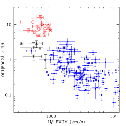
In all but 3 objects with strong and relatively narrow (FWHM$<$2000 km s^-1) permitted/semi-forbidden emission lines the H$\beta$ and [OIII]$\lambda$5007Å spectral region is covered. As discussed by several authors (e.g. Veron-Cetty & Veron 2003; Winkler 1992; Whittle 1992), a clear distinction between different types of AGN can be based on the ratio between [OIII]$\lambda$5007Å and H$\beta$ line intensity. Optically absorbed Seyferts, like Seyfert 2 or Seyfert1.8/1.9, present high values of the [OIII]$\lambda$5007Å /H$\beta$ flux ratios ($>$3), while moderately absorbed or non-absorbed Seyferts (Seyfert 1.5, Seyfert 1.2 and Seyfert 1 and NLSy1) show a [OIII]$\lambda$5007Å /H$\beta$ flux ratio between 0.2 and 3. In Figure 5 we show the [OIII]$\lambda$5007Å /H$\beta$ flux ratio versus the H$\beta$ width for all the XBS sources for which these lines are observed (including sources with FWHM$>$2000 km s^-1 emission lines). The two quantities are strongly coupled, and the objects with broad ($>$1000 km s^-1) H$\beta$ have all (but one) [OIII]$\lambda$5007Å /H$\beta$ flux ratio below 3. We classify all these objects type 1 AGN, including the source for which the [OIII]$\lambda$5007Å /H$\beta$ flux ratio is marginally greater than 3, since the value is consistent, within the errors, with those observed in type 1 AGN.

On the contrary, the objects with a narrow ($<$1000 km s^-1) H$\beta$ present a wide range of [OIII]$\lambda$5007Å /H$\beta$ flux ratios, from 0.3 to 15. This latter class of sources includes both type 2 AGN, “normal” galaxies (e.g. HII-region galaxies or starburst galaxies) and some NLSy1. To distinguish all these cases it is necessary to apply the diagnostic criteria discussed, e.g. in Veilleux & Osterbrock 1987, to separate type 2 AGN from HII-region/starburst galaxies, and/or the diagnostics based, for instance on the FeII$\lambda$4570Å /H$\beta$ flux ratio to recognize the NLSy1 (Véron-Cetty, Véron & Gonçalves 2001). The adopted criteria are indicated near the correspondent arrows of Fig. 4.

H$\beta$ and/or [OIII]$\lambda$5007Å not covered.

Only for 3 sources with strong and relatively narrow (FWHM$<$2000 km s^-1) permitted emission lines the H$\beta$/[OIII]$\lambda$5007Å spectral range is not covered. As discussed above these sources can be optically absorbed AGN (i.e. type 2 AGN) or NLQSO. The distinction between these two classes at large redshift is more critical than at lower z and other diagnostics must be used, like the intensity of the FeII$\lambda$4570Å hump or the relative strength of the HeII emission line when compared to the CIV$\lambda$1549Å (e.g. Heckman et al. 1995).

One of these objects (XBSJ021642.3–043553, z=1.985) has been extensively discussed in Severgnini et al. (2006) and it is classified as type 2 QSO on the basis of the relative strength of the HeII emission line when compared to the CIV$\lambda$1549Å.

The second source (XBSJ120359.1+443715, z=0.541) has a blue spectrum and a quite strong Fe II4570Å hump which is usually considered as the signature of a NLSy1. Unfortunately we cannot further quantify the strength of this hump in respect to the H$\beta$ line since this latter line falls outside the observed spectrum. We classify this object as NLQSO candidate.

Finally, in the third object (XBSJ124214.1–112512, z=0.82) we have detected the MgII$\lambda$2798Å emission line with a relatively narrow (FWHM$\sim$1900 km s^-1) core plus a broad wing. Both the FeII$\lambda$4570Å and the HeII line fall outside the observed range and we cannot apply the diagnostic criteria discussed above. Using the spectral model described in Section 8 we have successfully fitted the observed continuum emission using a value of A${}_{V}\sim$0.5 mag i.e. below the 2 mag limit that corresponds to our classification criteria (see Section 8). We thus classify this object as type 1 AGN.

7.4 Sources with weak (or absent) permitted emission lines

The last main “arrow” of Figure 4 corresponds to sources with no (or weak) permitted emission lines (excluding the H$\alpha$ line, as discussed above). This group of sources includes both “featureless” AGN (the BL Lac objects) and sources whose optical spectrum is dominated by the host-galaxy and no evidence (or little evidence) for the presence of an AGN can be inferred from the optical spectrum. As already discussed, these latter objects are considered as “elusive” AGN candidates and analysed separately using the X-ray information (see next sub-section).

BL Lac objects are classified on the basis of the lack of any (including the H$\alpha$) emission line and the shape of the continuum around the 4000Å break ($\Delta$ ). In fact the detection of a significant reduction of the 4000Å break when compared with elliptical galaxies is considered as an indication for the presence of nuclear emission. We adopt the limit commonly used in the literature of $\Delta<$40% to classify the source (with no-emission lines) as a BL Lac object (e.g. see the discussion in Landt et al. 2002).

The BL Lacs are 5 in total and all have been detected as radio sources in the NVSS (Condon et al. 1998) radio survey, something which is considered as a further confirmation of the correct classification. The properties of the XBS BL Lacs are presented in Galbiati et al. (2005). As discussed in Caccianiga et al. (2007) we cannot exclude that some of the “elusive” AGN are actually hiding a BL Lac nucleus. The best way to find them out is through a deep radio follow-up. On the basis of the current best estimate of the BL Lac sky density, however, we do not expect more than 1-2 BL Lacs hidden among the XBS elusive AGN.

7.5 The optically “elusive” AGN candidates

As summarized in Fig. 4, different classification paths lead to the group of optically “elusive” AGN candidates. All these sources (35 in total) are characterized by the presence, in the optical spectrum, of a significant/dominant contamination of star-light from the host galaxy. In some cases, i.e. for the so-called X-ray Bright Optically Normal Galaxies (XBONG) and the HII-region/starburst galaxies, we do not have clear (optical) evidence for the presence of an AGN. We consider as optically “elusive” AGN candidates also the sources where a broad ($>$1000-2000 km s^-1) H$\alpha$ line is probably present but where most of the remaining emission lines (in particular the H$\beta$ emission line) are not detected. Even if the presence of an AGN in these sources is somehow suggested by the detection of a broad H$\alpha$ emission line, the “dilution” due to the host galaxy is critical also in these cases because it does not permit a quantification of the optical absorption (i.e. type 1 or type 2 AGN). Similarly, some other sources in this group show a quite strong [OIII]$\lambda$5007Å , which can be suggestive of the presence of an AGN, but no H$\beta$ is detected, something that prevents us from a firm classification of the source.

Given the objective difficulty of using the optical spectra to assess the actual presence of an AGN and to give a correct classification of it (i.e. type 1, type 2 or BL Lac object) we have analyzed the X-ray data. In particular, we have shown that the X-ray spectral shape combined with the X-ray luminosity of the sources allows us to assess the presence of an AGN and to quantify its properties. While the detailed discussion of this analysis has been reported in Caccianiga et al. (2007) we summarize here the main conclusions. In the large majority of cases (33 out of 35 objects) the X-ray analysis has revealed an AGN while only in 2 cases the X-ray emission is probably due to the galaxy (either due to hot gas or to discrete sources) given the low X-ray luminosities (10³⁹-10⁴⁰ erg s^-1). In 20 sources where an AGN has been detected the column densities observed are below N_H=4$\times$10²¹ cm^-2 while in 12 the values are higher. Only for one object the data do not allow the estimate of the column density. According to the Galactic relationship between optical (A_V) and X-ray absorption (N_H) the value of N_H=4$\times$10²¹ cm^-2 corresponds to A${}_{V}\sim$2 mag which is the expected dividing line between type 1 and type 2 sources as defined in this paper, i.e. following the scheme of Fig. 4 (see the discussion in Section 8). We have thus classified these 32 “elusive” AGN into type 1 and type 2 according to the value of N_H measured from the X-ray analysis. In Tab 3 these classifications are flagged to indicate that they are not based on the optical spectra.

8 Diagnostic plots

Using a simple spectral model, discussed in Severgnini et al. (2003), we have produced some diagnostic plots that may help in the classification of X-ray selected sources. This model uses an AGN template composed of two parts: a) the continuum with the broad emission lines and b) the narrow emission lines. According to the basic version of the AGN unified model, the first part can be absorbed while the second one is not affected by the presence of an obscuring medium. The AGN template is based on the data taken from Francis et al. (1991) and Elvis et al. (1994) while the extinction curve is taken from Cardelli, Clayton & Mathis (1989). Besides the AGN template, the spectral model includes also a galaxy template, produced on the basis of the Bruzual & Charlot (2003) models.

We have then applied different levels of A_V and measured the expected values of some critical quantities like the 4000Å break, the [OIII]$\lambda$5007Å and the H$\alpha$ line equivalent width.

Figure 6: 4000Å break ($\Delta$) versus the [OIII]$\lambda$5007Å equivalent widths for the BSS type 1 (filled points) and type 2 (open circles) AGNs, excluding the elusive ones. The three lines show the expected regions corresponding to different optical absorptions, from A_V=1 mag to A_V=3 mag, assuming a 10 Gyr early-type host galaxy

Figure 7: Same plot as in fig. 6 but assuming a younger (1 Gyr) host-galaxy. Symbols as in Fig. 6.

8.1 Non-elusive AGN

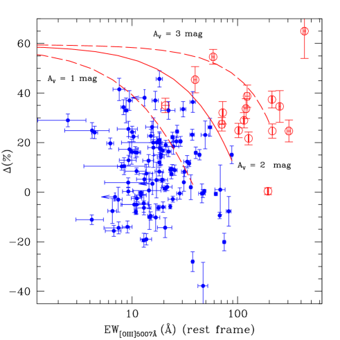
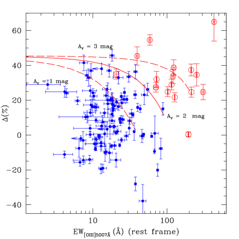
In Fig. 6 we have plotted the 4000Å break versus the [OIII]$\lambda$5007Å equivalent width of all the XBS sources classified as type 1 o type 2 AGN and for which these quantities have been computed, excluding the elusive AGN. On this plot type 2 and type 1 AGN occupy separated regions, with type 2 AGN showing the largest [OIII]$\lambda$5007Å equivalent widths and largest 4000Å breaks. This separation is expected since the presence of a large level of absorption in these sources significantly suppresses the AGN continuum, from the one hand, and increases the narrow lines equivalent widths, on the other hand. On the same figure we have then plotted the curves based on the spectral model described above for three different values of absorption, from A_V=1 mag to 3 mag, assuming a 10 Gyr old early-type host galaxy. The A_V=2 mag curve is clearly the one that better separates the two classes of AGNs. This result does not depend significantly on the host-galaxy type as shown in Fig. 7, where a much younger host-galaxy is assumed (1 Gyr). Also in this plot the line that better separates type 1 and type 2 AGN is the one corresponding to A_V=2 mag. This weak dependence with the host-galaxy type is not anymore true if we consider the elusive AGN i.e. those sources whose optical spectrum is dominated by the host-galaxy and that occupy the upper-left region of the diagram. Therefore, this plot cannot be used as diagnostic for the elusive AGN.

The clear separation between type 1 and type 2 AGN observed in a [OIII]$\lambda$5007Å/4000Å plot can be used as a simple diagnostic, at least for objects not dominated by the host-galaxy light. In Fig. 8 we report the typical regions occupied by type 1 and type 2 ANGs and (most of) the elusive AGN. This diagnostic diagram is simple to apply, requiring just the measure of the fluxes across the 4000Å break and the [OIII]$\lambda$5007Å equivalent width, and can be used up to z$\sim$0.8 (or higher if infrared spectra are available).

Figure 8: Typical regions occupied by the XBS AGNs on the 4000Å break/[OIII]$\lambda$5007Å EW plot

8.2 Elusive AGN with a broad H$\alpha$ emission line

By definition, elusive AGN have an optical spectrum which is dominated by the host galaxy light and, therefore, it is difficult/impossible to obtain a clear classification directly from the optical data. However, as already mentioned, in a number of elusive AGNs a possibly broad H$\alpha$ line in emission is found. In itself, this piece of information cannot give a clear indication of the type of AGN present in the source. With the support of the spectral model previously discussed we now want to find a method to estimate the level of optical absorption in these sources. We want to use only the few AGN emission lines that usually can be detected even in the presence of a high level of dilution, i.e. the [OIII]$\lambda$5007Å and the H$\alpha$ emission lines.

Figure 9: [OIII]$\lambda$5007Å  versus the H$\alpha$+[NII] line blend equivalent widths of the XBS AGN classified as type 1 and type 2 on the basis of the optical spectrum (panel a) and of the elusive AGN for which a broad H$\alpha$ emission line has been detected (panel b). In this case the classification is based on the X-ray spectrum. Open circles are type 2 AGN while filled points are type 1 AGN. Solid lines show the theoretical separation between objects with large ($A_{V}>$2 mag) and small ($A_{V}>$2 mag) optical absorption corresponding to a threshold of N_H=4$\times$10²¹ cm^-2 assuming a Galactic standard relation. The two lines correspond to different ages of the host-galaxy (t=1 Gyr and 10 Gyr respectively).

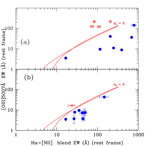
Interestingly, the combination of the H$\alpha$ line intensity with the [OIII]$\lambda$5007Å emission line can help the classification of the source. In Figure 9 we show the [OIII]$\lambda$5007Å  versus the H$\alpha$+[NII] blend equivalent widths of the XBS AGN classified as type 1 and type 2 on the basis of the optical spectrum (panel a). In panel (b) we report the 9 elusive AGN with a broad (FWHM$>$1000 km s^-1) H$\alpha$ emission line. In this case, the symbols represent a classification based on the X-ray spectral analysis, i.e. open symbols are AGN with N${}_{H}>$4$\times$10²¹ cm^-2 while filled circles are AGN with N${}_{H}<$4$\times$10²¹ cm^-2. On the two panels we report also the theoretical lines that separate between AGNs with large ($A_{V}>$2 mag) and small ($A_{V}<$2 mag) optical absorption (corresponding to N_H larger or lower than 4$\times$10²¹ cm^-2 assuming a Galactic standard relation). Each point of these lines corresponds to a different AGN-to-galaxy luminosity ratio (that increases from left to right).

In Figure 9b we do not include the sources classified as starburst or HII-region galaxies on the basis of the diagnostic diagrams because the H$\alpha$ line is likely to be produced within the host galaxy rather than by the AGN. We exclude also the sources with a narrow H$\alpha$ emission line to avoid sources whose H$\alpha$ line is contaminated by the emission from the host-galaxy. The solid line nicely separates the elusive objects affected by large absorption ($>$4$\times$10²¹ cm^-2) from those with low absorption ($<$4$\times$10²¹ cm^-2). More importantly, this separating line is fairly independent from the host-galaxy type even when the host galaxy light dominates the total spectrum (unlike the $\Delta$/[OIII]$\lambda$5007Å plot). Therefore, Figure 9 can be used as diagnostic tool to separate between type 1 and type 2 AGN, as defined in the XBS sample, when dilution from the host-galaxy does not allow to apply the usual diagnostic criteria and when X-ray data are not available.

9 The catalog

The result of the spectral classification of the XBS sources is summarized in Table 2 while in Table 3 we report the relevant optical information for each object. We note that the classification of the XBS sources has been presented in part in Della Ceca et al. (2004). The classification presented in that paper has been revised and refined to take into account the complexity of some spectra (like the presence of a significant star-light contribution) and, therefore, some of the published classifications (20 in total) have now changed. Most (14 out of 20) of the sources with a classification different from that presented in Della Ceca et al. (2004) are optically elusive AGN or “normal galaxies” and, therefore, the new classification is based on the X-ray spectrum. In Table 3 we have flagged the sources for which the classification presented here differs from that published in Della Ceca et al. (2004).

In Table 3 we have also listed an optical magnitude for each optical counterpart. As already discussed, we have not carried out a systematic photometric follow-up of the XBS sources and, therefore, the magnitudes are not homogeneous being taken from different catalogues/observations. For about half of the objects (172 objects) we have collected a red (R or r) magnitude either from our own observations or from existing catalogues (mostly the SDSS catalogue). Some of the R magnitudes derived from our own observations have been computed from the optical spectrum. Another substantial fraction of magnitudes (150) are taken from the APM facility (we use the red APM filter). For bright (and extended) objects the APM magnitude is known to suffer from a large systematic error. In these cases we have applied the correction described in Marchã et al. (2001) to compensate for this systematic error. Finally, for 26 objects classified as stars we have given the magnitude V or B present in Simbad.

10 The classification breakdown

Figure 10: Redshift distribution of the type 1 (solid line) and type 2 (dashed line) AGNs in the two samples (BSS and HBSS).

Figure 11: Magnitude vs. 2-7.5 keV flux (as derived from the count-rates) plot of the XBS extragalactic objects plus the unidentified sources: filled points = type 1 AGN, open circles = type 2 AGNs, open triangles = BL Lac objects, open squares = clusters of galaxies, stars = normal galaxies, crosses = unidentified sources. The continuous lines indicate the region of constant X-ray-to-optical flux ratio, from 0.01 to 100.

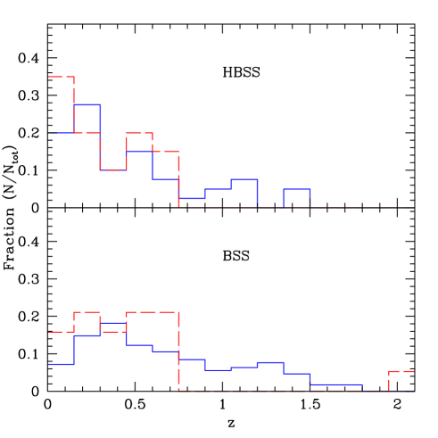
Table 2 reports the current classification breakdown of the sources in the BSS and HBSS samples. Given the high identification level (87% and 97% for the BSS and the HBSS samples respectively) the numbers in Table 2 should reflect the true relative compositions of the two samples. The first obvious consideration is that the percentage of stars decreases dramatically from the BSS sample (17%) to the HBSS sample (3%). Similarly, the relative fraction of type 2/type 1 AGN is significantly different in the 2 samples, being a factor 6 higher in the HBSS (0.48) than in the BSS (0.08). As expected, the 4.5-7.5 keV energy band is much more efficient in selecting type 2 AGN (efficiency $\sim$29%) when compared to the softer 0.5-4.5 keV band (efficiency$\sim$6%). It must be noted, however, that the optical recognition of the AGN in the hard energy band is more difficult when compared to the 0.5-4.5 keV band, since about 21% of the AGN are elusive (while only 10% of the AGN in the BSS are elusive). The different impact of the problem of dilution on type 1 and type 2 AGN and on different selection bands should be kept in mind when deriving statistical considerations on the populations of AGNs present in X-ray surveys.

As far as the BL Lac objects are concerned the selection efficiency in the 0.5-4.5 keV band is about 1-2%. If this efficiency was the same in the 4.5-7.5 keV band we would expect $\sim$1 BL Lac, something that is statistically consistent with the fact that no BL Lacs are observed in the HBSS sample.

The redshift distribution of type 1 and type 2 AGN in the two samples is shown in Figure 10. In the BSS sample, the mean redshift of type 1 AGNs ($<z>_{Ty1}$=0.69$\pm$0.03) is significantly different from the mean redshift of type 2 AGNs ($<z>_{Ty2}$=0.47$\pm$0.10) while they are closer in the HBSS sample ($<z>_{Ty1}$=0.47$\pm$0.06 $<z>_{Ty2}$=0.33$\pm$0.05). A K-S test confirms that the z-distribution of the two classes of AGN are consistent with being derived from the same parent distribution when considering the HBSS sample (K-S probability=33%) while they are significantly different (at 95% confidence level) when considering the BSS sample (K-S probability=1.6%). This result probably reflects the fact that the hard-energy (4.5-7.5 keV) selection is less biased in respect to the obscuration (at least in the Compton-thin regime) when compared to a softer (0.5-4.5 keV) energy selection.

Finally, in Fig. 11 we plot the extragalactic XBS sources and the unidentified objects on the magnitude/X-ray flux diagram. The identified extragalactic sources, with the exception of three objects, have an X-ray-to-optical flux ratio (X/O) between 0.005 and 20. At the two “extreme” sides of the distribution we find the two “normal” galaxies, that have the lowest values of X/O ($\sim$10^-4) similar to those observed in some stars, and, on the other side of the distribution, the high z type 2 QSO, discussed in Severgnini et al. (2006), which has the highest value of X/O ($\sim$200). Among the unidentified sources we have at least one object whose lower limit on the magnitude (R$>$22.8) implies a X/O greater than 60, making it an excellent candidate of high-z type 2 QSO.

Interestingly enough, among the high ($>$10) X/O sources 3 type 1 AGN are found. These objects represent a non negligible fraction considering that about half of the high X/O sources are still unidentified and more cases like these may show up after the completion of the spectroscopic follow-up. A significant presence of type 1 AGN among high X/O sources has been found also at lower X-ray fluxes ($\sim$10^-14 erg s^-1 cm^-2) in the XMM-Newton Medium sensitivity Survey (XMS, Barcons et al. 2007).

Table 2: Breakdown of the optical classification. Numbers between parenthesis indicate the number of sources for which the classification is based on the X-ray spectral analysis (see Caccianiga et al. 2007)

Type	Number	in BSS	in HBSS
AGN 1	245 (20)	244 (20)	42 (4)
AGN 2	29 (12)	19 (5)	20 (9)
AGN (uncertain type)	1 (1)	1 (1)	0
BL Lacs	5	5	0
“normal” Galaxies	2 (2)	2 (2)	0
Clusters of galaxies	8	8	1
stars	58	58	2
IDs	348 (35)	337 (28)	65 (13)
total	400	389	67

11 Summary and conclusions

We have presented the details of the identification work of the sources in the XBS survey, which is composed by two complete flux limited samples, the BSS and the HBSS sample, selected in the 0.5-4.5 keV and 4.5-7.5 keV band respectively. We have secured a redshift and a spectroscopic classification for 348 (including data from the literature) out of 400 sources, corresponding to 87% of the total list of sources and to 87% and 97% considering the BSS and HBSS samples separately.

The results of the identification work can be summarized as follows:

• We have quantified the criteria used to distinguish optically absorbed AGN (i.e. type 2) from optically non-absorbed (or moderately absorbed) AGN (type 1) and we have shown that the adopted dividing line between the two classes of sources corresponds to an optical extinction of A${}_{V}\sim$2 mag, which translates into an expected column density of N${}_{H}\sim$4$\times$10²¹ cm^-2, assuming a Galactic A_V/N_H relationship.

• About 10% of the extragalactic sources (35 objects in total) show an optical spectrum which is highly contaminated by the star-light from the host galaxy. These sources have been studied in detail in a companion paper (Caccianiga et al. 2007). Using the X-ray data we have found an elusive AGN in 33 of these objects and we have classified them into type 1 and type 2 AGN according to the value of N_H measured from the X-ray spectrum. To this end, we have used a N_H=4$\times$10²¹ cm^-2 dividing value which matches (assuming the standard Galactic A_V/N_H relation) the value of A_V (=2 mag) adopted with the optical classification.

• We have then proposed two simple diagnostic diagrams. The first one, based on the 4000Å break and the [OIII]$\lambda$5007Å equivalent width, can reliably distinguish between type 1 and type 2 AGN if the host galaxy does not dominate the optical spectrum. The second uses the H$\alpha$ and [OIII]$\lambda$5007Å line equivalent widths to classify into type 1 and type 2 the elusive AGN sources in which a possibly broad H$\alpha$ emission line is detected.

• We find that the AGN represent the most numerous population at the flux limit of the XBS survey ($\sim$10^-13 erg cm^-2 s^-1) constituting 80% of the XBS sources selected in the 0.5-4.5 keV energy band and 95% of the “hard” (4.5-7.5 keV) selected objects. Galactic sources populate significantly the 0.5-4.5 keV sample (17%) and only marginally (3%) the 4.5-7.5 keV sample. The remaining sources in both samples are clusters/groups of galaxies and normal galaxies (i.e. probably not powered by an AGN).

• As expected, the percentage of type 2 AGN dramatically increases going from the 0.5-4.5 keV sample (f=N_AGN2/N_AGN=7%) to the 4.5-7.5 keV sample (f=32%). A detailed analysis on the intrinsic (i.e. taking into account the selection effects) relative fraction of type 1 and type 2 AGN will be be presented in a forthcoming paper (Della Ceca et al. 2007, in prep.).

Table 3: Optical properties of the XBSS sources

name	Sample	Optical position	Class	flag class	z	mag	flag mag	reference
		(J2000)
XBSJ000027.7–250442	bss	00 00 27.68 –25 04 42.8	AGN1		0.336	19.0	3	1
XBSJ000031.7–245502	bss	00 00 31.89 –24 54 59.5	AGN1		0.284	17.2	1	1
XBSJ000100.2–250501	bss	00 01 00.23 –25 05 01.5	AGN1		0.850	20.4	3	1
XBSJ000102.4–245850	bss	00 01 02.46 –24 58 49.6	AGN1		0.433	20.3	1	1
XBSJ000532.7+200716	bss	00 05 32.84 +20 07 17.4	AGN1	1 3	0.119	17.9	3	obs
XBSJ001002.4+110831	bss	00 10 02.66 +11 08 34.4	star		–	5.5	5	43
XBSJ001051.6+105140	bss	00 10 51.41 +10 51 40.5	star		–	15.8	4	obs
XBSJ001749.7+161952	bss	00 17 49.93 +16 19 56.1	star		–	7.2	5	43
XBSJ001831.6+162925	bss	00 18 32.02 +16 29 25.9	AGN1		0.553	18.3	3	42,2
XBSJ002618.5+105019	bss,hbss	00 26 18.71 +10 50 19.6	AGN1		0.473	17.5	3	obs
XBSJ002637.4+165953	bss	00 26 37.46 +16 59 54.4	AGN1		0.554	18.9	3	obs
XBSJ002707.5+170748	bss	00 27 07.78 +17 07 50.5	AGN1		0.930	20.2	1	obs
XBSJ002953.1+044524	bss	00 29 53.16 +04 45 24.1	star		–	9.5	6	43
XBSJ003255.9+394619	bss	00 32 55.73 +39 46 19.4	AGN1		1.139	17.7	3	obs
XBSJ003315.5–120700	bss	00 33 15.63 –12 06 58.7	AGN1		1.206	19.8	3	obs
XBSJ003316.0–120456	bss	00 33 16.04 –12 04 56.2	AGN1		0.660	18.9	3	obs
XBSJ003418.9–115940	bss	00 34 19.00 –11 59 38.2	AGN1		0.850	20.6	1	obs
XBSJ005009.9–515934	bss	00 50 09.66 –51 59 32.4	AGN1		0.610	20.1	3	obs
XBSJ005031.1–520012	bss	00 50 30.85 –52 00 09.8	AGN1		0.463	18.7	3	obs
XBSJ005032.3–521543	bss	00 50 32.13 –52 15 42.3	AGN1		1.216	19.9	3	obs
XBSJ005822.9–274016	bss	00 58 22.96 –27 40 14.2	star		–	12.3	5	43
XBSJ010421.4–061418	bss	01 04 21.57 –06 14 17.5	AGN1		0.520	21.2	2	obs
XBSJ010432.8–583712	bss	01 04 32.64 –58 37 11.2	AGN1		1.640	19.3	3	obs
XBSJ010701.5–172748	bss	01 07 01.47 –17 27 46.4	AGN1		0.890	19.2	3	obs
XBSJ010747.2–172044	bss	01 07 47.50 –17 20 42.0	AGN1		0.980	17.5	3	obs
XBSJ012000.0–110429	bss	01 20 00.10 –11 04 30.0	AGN1		0.351	20.3	3	obs
XBSJ012025.2–105441	bss	01 20 25.31 –10 54 38.6	AGN1		1.338	18.9	3	3,39
XBSJ012057.4–110444	bss	01 20 57.38 –11 04 44.0	AGN2		0.072	16.7	1	obs
XBSJ012119.9–110418	bss	01 21 19.99 –11 04 14.9	AGN1		0.204	17.5	4	obs
XBSJ012505.4+014624	bss	01 25 05.50 +01 46 27.2	AGN1		1.567	19.0	3	obs
XBSJ012540.2+015752	bss	01 25 40.36 +01 57 53.8	AGN1	1 3	0.123	17.3	4	obs
XBSJ012654.3+191246	bss	01 26 54.45 +19 12 52.5	AGN1	1 3	0.043	13.7	1	obs
XBSJ012757.2+190000	bss	01 27 57.05 +19 00 02.0	star		–	12.7	5	41
XBSJ012757.3+185923	bss	01 27 57.24 +18 59 26.3	star		–	9.4	5	43
XBSJ013204.9–400050	bss	01 32 05.19 –40 00 48.2	AGN1		0.450	19.1	3	obs
XBSJ013240.1–133307	bss,hbss	01 32 40.29 –13 33 06.5	AGN2		0.562	20.0	3	obs
XBSJ013811.7–175416	bss	01 38 11.72 –17 54 13.4	BL		0.530	19.2	3	obs
XBSJ013944.0–674909	bss,hbss	01 39 43.70 –67 49 08.1	AGN1	1	0.104	17.7	4	obs
XBSJ014100.6–675328	bss,hbss	01 41 00.29 –67 53 27.5	star		–	16.4	3	obs
XBSJ014109.9–675639	bss	01 41 09.53 –67 56 38.7	AGN1	1	0.226	19.2	3	obs
XBSJ014227.0+133453	bss	01 42 27.31 +13 34 53.1	AGN1	1 3	0.275	19.3	2	obs
XBSJ014251.5+133352	bss	01 42 51.72 +13 33 52.7	AGN1		1.071	19.0	2	obs
XBSJ015916.9+003010	bss	01 59 17.20 +00 30 13.0	CL		0.382	17.8	2	obs
XBSJ015957.5+003309	bss,hbss	01 59 57.65 +00 33 10.8	AGN1		0.310	18.8	2	obs
XBSJ020029.0+002846	bss	02 00 29.07 +00 28 46.7	AGN1		0.174	18.0	2	obs
XBSJ020757.3+351828	bss	02 07 57.15 +35 18 28.2	AGN1		0.188	18.3	3	obs
XBSJ020845.1+351438	bss	02 08 44.96 +35 14 37.2	AGN1		0.415	19.1	3	obs
XBSJ021640.7–044404	bss,hbss	02 16 40.72 –04 44 04.8	AGN1		0.873	17.2	4	obs
XBSJ021642.3–043553	bss	02 16 42.36 –04 35 51.9	AGN2		1.985	24.5	1	obs
XBSJ021808.3–045845	bss,hbss	02 18 08.24 –04 58 45.2	AGN1		0.712	17.7	3	40
XBSJ021817.4–045113	bss,hbss	02 18 17.45 –04 51 12.4	AGN1		1.080	19.5	3	40
XBSJ021820.6–050427	bss	02 18 20.46 –05 04 26.2	AGN1		0.646	18.7	3	obs
XBSJ021822.2–050615	hbss	02 18 22.16 –05 06 14.4	AGN2	1	0.044	15.2	1	obs
XBSJ021830.0–045514	bss	02 18 29.91 –04 55 13.8	star		–	14.3	1	40
XBSJ021923.2–045148	bss	02 19 23.30 –04 51 48.6	AGN1		0.632	18.9	3	obs
XBSJ022253.0–044515	bss	02 22 53.15 –04 45 13.1	AGN1		1.420	20.5	1	obs

Table 3: continue

name	Sample	Optical position	Class	flag class	z	mag	flag mag	reference
		(J2000)
XBSJ022707.7–050819	bss	02 27 07.93 –05 08 17.4	AGN2		0.358	18.9	3	obs
XBSJ023459.7–294436	bss	02 34 59.97 –29 44 34.6	AGN1		0.446	17.7	3	obs
XBSJ023530.2–523045	bss	02 35 30.38 –52 30 43.2	AGN1		0.429	18.8	3	obs
XBSJ023713.5–522734	bss,hbss	02 37 13.57 –52 27 34.1	AGN1		0.193	17.1	3	obs
XBSJ023853.2–521911	bss	02 38 53.41 –52 19 09.9	AGN1		0.648	19.4	3	obs
XBSJ024200.9+000020	bss	02 42 00.91 +00 00 21.1	AGN1	2	1.112	18.4	2	4
XBSJ024204.7+000814	bss	02 42 04.77 +00 08 14.7	AGN1		0.383	18.9	2	obs
XBSJ024325.6–000413	bss	02 43 25.50 –00 04 13.0	AGN1		0.356	19.4	3	obs
XBSJ025606.1+001635	bss	02 56 06.00 +00 16 34.8	AGN1		0.629	20.1	2	obs
XBSJ025645.4+000031	bss	02 56 45.29 +00 00 33.2	AGN1	1	0.359	19.3	2	obs
XBSJ030206.8–000121	bss,hbss	03 02 06.77 –00 01 21.1	AGN1	2	0.641	18.8	3	6
XBSJ030614.1–284019	bss,hbss	03 06 14.17 –28 40 20.1	AGN1		0.278	18.5	3	obs
XBSJ030641.0–283559	bss	03 06 41.10 –28 35 58.8	AGN1		0.367	17.3	3	obs
XBSJ031015.5–765131	bss,hbss	03 10 15.69 –76 51 32.9	AGN1		1.187	17.6	3	7
XBSJ031146.1–550702	bss,hbss	03 11 46.08 –55 07 00.2	AGN2		0.162	17.3	3	obs
XBSJ031311.7–765428	bss	03 13 11.85 –76 54 30.4	AGN1		1.274	19.1	3	7
XBSJ031401.3–545959	bss	03 14 01.37 –54 59 56.4	AGN1		0.841	20.2	3	8
XBSJ031549.4–551811	bss	03 15 49.60 –55 18 13.0	AGN1		0.808	20.3	3	8
XBSJ031851.9–441815	bss	03 18 52.04 –44 18 16.7	AGN1		1.360	19.0	3	obs
XBSJ031859.2–441627	bss,hbss	03 18 59.46 –44 16 26.4	AGN1	1	0.140	16.7	1	obs
XBSJ033208.7–274735	bss	03 32 08.67 –27 47 34.3	AGN1	3	0.544	18.3	3	9,10
XBSJ033226.9–274107	bss	03 32 27.03 –27 41 04.8	AGN1		0.736	18.8	3	obs
XBSJ033435.5–254259	bss	03 34 35.76 –25 42 54.9	AGN1		1.190	19.4	3	obs
XBSJ033453.9–254154	bss	03 34 54.14 –25 41 53.2	AGN1		1.160	18.6	3	obs
XBSJ033506.0–255619	bss	03 35 06.02 –25 56 19.3	AGN1		1.430	17.4	3	obs
XBSJ033845.7–352253	hbss	03 38 46.01 –35 22 52.2	AGN2		0.113	17.0	3	obs
XBSJ033851.4–352646	bss	03 38 51.60 –35 26 44.7	AGN1		1.070	19.5	1	obs
XBSJ033912.1–352813	bss	03 39 12.18 –35 28 12.4	AGN1		0.466	19.7	1	obs
XBSJ033942.8–352411	bss	03 39 42.90 –35 24 10.3	AGN1		1.043	19.0	3	11
XBSJ040658.8–712457	hbss	04 06 58.85 –71 24 59.6	AGN2		0.181	18.7	3	obs
XBSJ040744.6–710846	bss	04 07 44.56 –71 08 47.5	star		–	17.9	3	obs
XBSJ040758.9–712833	hbss	04 07 58.53 –71 28 32.9	AGN2		0.134	17.0	3	obs
XBSJ040807.2–712702	bss	04 08 07.08 –71 27 01.6	star		–	12.4	4	43
XBSJ041108.1–711341	bss,hbss	04 11 08.59 –71 13 43.0	AGN1		0.923	20.3	1	obs
XBSJ043448.3–775329	bss	04 34 47.78 –77 53 28.3	AGN1	1	0.097	17.7	3	obs
XBSJ045942.4+015843	bss	04 59 42.50 +01 58 44.2	AGN1		0.248	19.1	3	obs
XBSJ050011.7+013948	bss	05 00 11.72 +01 39 48.8	AGN1		0.360	19.9	3	obs
XBSJ050446.3–283821	bss	05 04 46.38 –28 38 20.1	AGN1		0.840	20.6	1	obs
XBSJ050453.4–284532	bss	05 04 53.35 –28 45 31.0	AGN1	1	0.204	19.0	1	obs
XBSJ050501.8–284149	bss	05 05 01.90 –28 41 48.5	AGN1		0.257	18.8	1	obs
XBSJ050536.6–290050	bss,hbss	05 05 36.56 –29 00 49.7	AGN2		0.577	21.2	1	obs
XBSJ051617.1+794408	bss	05 16 17.23 +79 44 11.0	star		–	9.3	5	43
XBSJ051655.3–104104	bss	05 16 55.28 –10 41 02.4	AGN1		0.568	20.3	1	obs
XBSJ051822.6+793208	bss	05 18 22.55 +79 32 09.8	AGN1	1 3	0.053	15.0	4	obs
XBSJ051955.5–455727	bss	05 19 55.56 –45 57 25.2	AGN1		0.562	19.0	1	obs
XBSJ052022.0–252309	bss	05 20 22.17 –25 23 10.5	AGN1		0.745	19.8	1	obs
XBSJ052048.9–454128	bss	05 20 49.30 –45 41 30.2	star		–	11.9	5	43
XBSJ052108.5–251913	bss,hbss	05 21 08.71 –25 19 13.3	AGN1		1.196	17.5	3	obs
XBSJ052116.2–252957	bss	05 21 16.08 –25 29 58.3	AGN1	1	0.332	19.6	1	obs
XBSJ052128.9–253032	hbss	05 21 29.04 –25 30 32.3	AGN2	1	0.588	20.8	1	obs
XBSJ052144.1–251518	bss	05 21 44.37 –25 15 23.0	AGN1		0.321	18.9	1	obs
XBSJ052155.0–252200	bss	05 21 55.32 –25 22 00.9	star		–	13.0	1	41
XBSJ052509.3–333051	bss	05 25 09.29 –33 30 52.9	CL		0.704	21.2	1	obs
XBSJ052543.6–334856	bss	05 25 43.61 –33 48 57.5	AGN1		0.735	19.7	1	obs
XBSJ061342.7+710725	bss	06 13 43.20 +71 07 24.6	BL		0.267	16.6	4	12
XBSJ062134.8–643150	bss	06 21 34.74 –64 31 51.5	AGN1		1.277	18.0	3	obs

Table 3: continue

name	Sample	Optical position	Class	flag class	z	mag	flag mag	reference
		(J2000)
XBSJ062425.7–642958	bss	06 24 25.78 –64 29 58.3	star		–	11.1	5	43
XBSJ065214.1+743230	bss	06 52 14.62 +74 32 29.4	AGN1		0.620	19.9	3	obs
XBSJ065237.4+742421	bss	06 52 37.62 +74 24 20.2	CL		0.360	19.0	1	obs
XBSJ065400.0+742045	bss	06 54 00.28 +74 20 44.0	AGN1		0.362	19.3	1	obs
XBSJ065744.3–560817	bss	06 57 44.17 –56 08 18.8	AGN1		0.120	17.1	1	obs
XBSJ065839.5–560813	bss	06 58 39.33 –56 08 12.2	AGN1		0.211	17.3	1	obs
XBSJ074202.7+742625	bss,hbss	07 42 02.68 +74 26 24.7	AGN1		0.599	20.9	1	obs
XBSJ074312.1+742937	bss,hbss	07 43 12.60 +74 29 36.3	AGN1		0.312	17.1	4	13
XBSJ074338.7+495431	bss	07 43 38.99 +49 54 28.5	AGN1		0.221	19.2	2	obs
XBSJ074352.0+744258	bss	07 43 52.98 +74 42 57.9	AGN1		0.800	18.8	2	40
XBSJ074359.7+744057	bss	07 44 00.55 +74 40 56.5	star		–	14.6	4	obs
XBSJ075117.9+180856	bss	07 51 17.96 +18 08 56.0	AGN1	1	0.255	18.7	2	obs
XBSJ080309.8+650807	bss	08 03 09.11 +65 08 06.7	star		–	7.7	5	43
XBSJ080608.1+244420	bss	08 06 08.15 +24 44 21.3	AGN1		0.357	18.3	2	obs
XBSJ083737.0+255151	bss,hbss	08 37 37.04 +25 51 51.6	AGN1	1 3	0.105	16.5	2	obs
XBSJ083737.1+254751	bss,hbss	08 37 37.08 +25 47 50.5	AGN1		0.080	16.8	2	13,39
XBSJ083838.6+253616	bss	08 38 38.48 +25 36 17.1	AGN1		0.601	19.2	2	obs
XBSJ083905.9+255010	bss	08 39 05.91 +25 50 09.3	AGN1		0.250	20.0	2	obs
XBSJ084026.2+650638	bss	08 40 26.11 +65 06 38.3	AGN1		1.144	18.7	1	obs
XBSJ084651.7+344634	bss	08 46 51.68 +34 46 34.7	AGN1		1.115	18.1	3	42
XBSJ085427.8+584158	bss	08 54 28.24 +58 42 05.3	star		–	10.0	5	43
XBSJ085530.7+585129	bss	08 55 30.97 +58 51 29.0	AGN1		0.905	21.4	2	obs
XBSJ090729.1+620824	bss	09 07 29.30 +62 08 27.0	AGN2	1 3	0.388	20.4	2	obs
XBSJ091043.4+054757	bss	09 10 43.33 +05 48 01.8	star		–	17.5	2	obs
XBSJ091828.4+513931	bss,hbss	09 18 28.59 +51 39 32.3	AGN1		0.185	17.1	2	obs
XBSJ094526.2–085006	bss	09 45 26.25 –08 50 05.9	AGN1	1	0.314	18.2	1	obs
XBSJ094548.3–084824	bss	09 45 48.18 –08 48 23.7	AGN1		1.748	18.6	3	obs
XBSJ095054.5+393924	bss	09 50 54.88 +39 39 27.4	AGN1		1.299	19.6	2	obs
XBSJ095218.9–013643	bss,hbss	09 52 19.08 –01 36 43.4	AGN1		0.020	13.7	4	14
XBSJ095309.7+013558	bss	09 53 10.13 +01 35 56.6	AGN1		0.477	19.3	1	obs
XBSJ095341.1+014204	bss	09 53 41.36 +01 42 02.4	CL		0.090	14.8	2	obs
XBSJ095416.9+173627	bss	09 54 16.74 +17 36 28.4	CL		–	20.2	2	obs
XBSJ095509.6+174124	bss	09 55 09.63 +17 41 24.9	AGN1		1.290	20.1	2	obs
XBSJ095955.2+251549	bss	09 59 55.07 +25 15 51.7	star		–	11.8	2	obs
XBSJ100032.5+553626	bss	10 00 32.29 +55 36 30.6	AGN2	1	0.216	17.9	2	15,16,39
XBSJ100100.0+252103	bss	10 01 00.12 +25 21 04.9	AGN1		0.794	19.4	2	obs
XBSJ100309.4+554135	bss	10 03 09.45 +55 41 34.5	AGN1		0.673	19.0	2	15,16,39
XBSJ100828.8+535408	bss	10 08 28.95 +53 54 05.8	AGN1		0.384	18.7	1	obs
XBSJ100921.7+534926	bss	10 09 21.88 +53 49 25.5	AGN1		0.387	18.9	2	15,16,39
XBSJ100926.5+533426	bss	10 09 26.75 +53 34 24.3	AGN1		1.718	19.3	2	15,16,39
XBSJ101506.0+520157	bss	10 15 06.05 +52 01 58.2	AGN1		0.610	19.6	2	obs
XBSJ101511.8+520708	bss	10 15 11.96 +52 07 07.2	AGN1		0.888	20.5	2	obs
XBSJ101706.5+520245	bss	10 17 06.69 +52 02 47.2	BL		0.377	18.8	2	obs
XBSJ101838.0+411635	bss	10 18 37.99 +41 16 38.3	AGN1		0.577	19.8	2	obs
XBSJ101843.0+413515	bss	10 18 43.16 +41 35 16.5	AGN1	1 3	0.084	15.9	2	obs
XBSJ101850.5+411506	bss,hbss	10 18 50.53 +41 15 08.3	AGN1		0.577	18.4	2	obs
XBSJ101922.6+412049	bss,hbss	10 19 22.73 +41 20 50.1	AGN1		0.239	18.5	2	obs
XBSJ102044.1+081424	bss	10 20 44.17 +08 14 23.8	star		–	15.2	4	obs
XBSJ102412.3+042023	bss	10 24 12.33 +04 20 25.8	AGN1		1.458	19.5	2	obs
XBSJ102417.5+041656	bss	10 24 17.46 +04 16 57.8	AGN1		1.712	20.1	2	obs
XBSJ103154.1+310732	bss	10 31 54.12 +31 07 31.3	AGN1		0.299	18.8	2	40
XBSJ103745.7+532353	bss	10 37 45.51 +53 23 53.0	AGN1		2.347	19.8	2	obs
XBSJ103932.7+205426	bss	10 39 32.68 +20 54 27.6	AGN1		0.237	18.8	2	obs
XBSJ103935.8+533036	bss	10 39 35.75 +53 30 38.6	AGN1		0.229	18.4	2	obs
XBSJ104026.9+204542	bss,hbss	10 40 26.84 +20 45 44.5	AGN1		0.465	19.8	2	obs
XBSJ104425.0–013521	bss	10 44 24.87 –01 35 19.5	AGN1		1.571	19.0	3	9

Table 3: continue

name	Sample	Optical position	Class	flag class	z	mag	flag mag	reference
		(J2000)
XBSJ104509.3–012442	bss	10 45 09.32 –01 24 42.5	AGN1		0.472	20.0	1	obs
XBSJ104522.1–012843	bss,hbss	10 45 22.09 –01 28 44.5	AGN1	2	0.782	19.4	3	9
XBSJ104912.8+330459	bss,hbss	10 49 12.58 +33 05 01.3	AGN1		0.226	18.6	2	obs
XBSJ105131.1+573439	bss	10 51 31.25 +57 34 38.8	star		–	14.7	3	obs
XBSJ105239.7+572431	bss	10 52 39.76 +57 24 30.6	AGN1		1.113	17.8	2	17,39
XBSJ105316.9+573551	bss	10 53 16.97 +57 35 50.1	AGN1		1.204	18.8	3	17,39
XBSJ105335.0+572540	bss	10 53 35.10 +57 25 42.3	AGN1		0.784	21.1	2	17
XBSJ105339.7+573104	bss	10 53 39.80 +57 31 03.9	AGN1		0.586	19.8	2	17
XBSJ105624.2–033522	bss	10 56 24.00 –03 35 26.6	AGN1		0.635	19.0	1	obs
XBSJ110320.1+355803	bss	11 03 20.05 +35 58 04.2	star		–	7.5	5	43
XBSJ111654.8+180304	bss	11 16 54.72 +18 03 05.9	G	1 3	0.003	10.6	2	18
XBSJ111928.5+130250	bss	11 19 28.39 +13 02 51.3	AGN1		2.394	18.0	2	obs
XBSJ111933.0+212756	bss	11 19 33.22 +21 27 57.6	AGN1		0.282	19.2	2	15,16
XBSJ111942.1+211516	bss	11 19 42.14 +21 15 16.8	AGN1		1.288	20.0	2	15,16
XBSJ112022.3+125252	bss	11 20 22.37 +12 52 50.6	AGN1		0.406	18.9	3	obs
XBSJ112026.7+431520	hbss	11 20 26.62 +43 15 18.2	AGN2	1	0.146	17.5	2	obs
XBSJ112046.7+125429	bss	11 20 46.75 +12 54 29.5	AGN1		0.382	19.4	2	obs
XBSJ113106.9+312518	bss,hbss	11 31 06.94 +31 25 19.6	AGN1		1.482	19.4	2	obs
XBSJ113121.8+310252	bss,hbss	11 31 21.81 +31 02 54.8	AGN2		0.190	18.5	2	40
XBSJ113128.6–195903	bss	11 31 28.44 –19 59 03.2	AGN1		0.363	18.6	3	obs
XBSJ113148.7+311358	bss,hbss	11 31 48.66 +31 14 01.3	AGN2		0.500	20.4	2	42
XBSJ113837.9–373402	bss	11 38 37.74 –37 33 59.9	AGN1		0.120	18.3	3	obs
XBSJ115846.9+551625	bss	11 58 47.01 +55 16 24.3	AGN1		0.518	19.6	2	15,16
XBSJ120359.1+443715	bss	12 03 59.10 +44 37 14.8	AGN1		0.641	19.5	2	obs
XBSJ120413.7+443149	bss	12 04 13.72 +44 31 47.6	AGN1		0.492	19.9	2	obs
XBSJ122017.5+752217	bss	12 20 17.76 +75 22 15.2	G	1	0.006	11.7	2	19
XBSJ122350.4+752231	bss	12 23 50.97 +75 22 28.6	AGN1		0.565	18.8	3	40
XBSJ122655.1+012002	bss	12 26 54.98 +01 20 00.9	star		–	18.2	2	obs
XBSJ122656.5+013126	bss,hbss	12 26 56.46 +01 31 24.4	AGN2		0.733	20.2	2	obs
XBSJ122658.1+333246	bss	12 26 58.20 +33 32 49.0	CL		0.891	20.6	2	20,21
XBSJ122751.2+333842	bss	12 27 51.17 +33 38 46.5	star		–	15.4	4	obs
XBSJ122837.3+015720	bss	12 28 37.24 +01 57 19.5	star		–	13.4	2	42
XBSJ122942.3+015525	bss	12 29 42.48 +01 55 24.9	star		–	14.4	2	obs
XBSJ123116.5+641115	bss	12 31 16.50 +64 11 14.4	AGN1		0.454	20.8	2	40
XBSJ123208.7+640304	bss	12 32 08.89 +64 03 02.6	star		–	14.8	2	obs
XBSJ123218.5+640311	bss	12 32 18.83 +64 03 09.8	AGN1		1.013	21.0	2	40
XBSJ123538.6+621644	bss	12 35 38.52 +62 16 43.5	AGN1		0.717	20.0	2	obs
XBSJ123549.1–395026	bss	12 35 49.00 –39 50 24.3	star		–	12.4	1	41
XBSJ123600.7–395217	bss,hbss	12 36 00.55 –39 52 15.1	star		–	5.8	5	43
XBSJ123759.6+621102	bss	12 37 59.57 +62 11 02.5	AGN1		0.910	18.4	2	22,39
XBSJ123800.9+621338	bss	12 38 00.92 +62 13 36.0	AGN1		0.440	18.8	2	23,39
XBSJ124214.1–112512	bss	12 42 13.79 –11 25 10.6	AGN1		0.820	18.5	3	obs
XBSJ124557.6+022659	bss	12 45 57.49 +02 26 57.2	AGN1		0.708	19.7	1	obs
XBSJ124607.6+022153	bss	12 46 07.49 +02 21 53.2	AGN1		0.491	19.7	2	obs
XBSJ124641.8+022412	bss,hbss	12 46 41.70 +02 24 11.3	AGN1		0.934	17.5	2	24,39
XBSJ124647.9+020955	bss	12 46 47.91 +02 09 54.3	AGN1		1.074	19.6	1	obs
XBSJ124903.6–061049	bss	12 49 03.49 –06 10 47.3	AGN1		0.646	19.1	3	obs
XBSJ124914.6–060910	bss	12 49 14.60 –06 09 09.6	AGN1		1.627	18.9	3	obs
XBSJ124938.7–060444	bss	12 49 38.66 –06 04 44.2	star		–	9.7	5	43
XBSJ124949.4–060722	bss	12 49 49.44 –06 07 22.9	AGN1		1.053	18.6	1	obs
XBSJ125457.2+564940	bss	12 54 56.78 +56 49 41.8	AGN1		1.261	20.3	2	15,16,39
XBSJ130619.7–233857	bss	13 06 19.57 –23 38 56.9	AGN1		0.351	18.4	1	obs
XBSJ130658.1–234849	bss	13 06 58.05 –23 48 47.3	AGN1		0.375	18.4	3	obs
XBSJ132038.0+341124	bss,hbss	13 20 37.88 +34 11 26.2	AGN1		0.065	16.0	2	42
XBSJ132052.5+341742	bss	13 20 52.56 +34 17 44.1	AGN1		0.844	21.0	2	42
XBSJ132101.6+340656	bss	13 21 01.43 +34 06 58.0	AGN1		0.335	18.6	2	42

Table 3: continue

name	Sample	Optical position	Class	flag class	z	mag	flag mag	reference
		(J2000)
XBSJ132105.5+341459	bss	13 21 05.52 +34 15 01.0	AGN1		0.452	20.3	2	42
XBSJ133023.8+241707	bss	13 30 23.77 +24 17 08.5	AGN1		1.438	19.3	2	obs
XBSJ133026.6+241520	bss	13 30 26.53 +24 15 21.8	BL		0.460	19.2	2	obs
XBSJ133321.2+503102	bss	13 33 21.36 +50 31 06.2	star		–	11.1	5	obs
XBSJ133626.9–342636	bss	13 36 27.00 –34 26 33.0	star		–	13.4	4	41
XBSJ133807.5+242411	bss	13 38 07.52 +24 24 11.7	AGN1		0.631	18.0	2	obs
XBSJ133942.6–315004	bss,hbss	13 39 42.47 –31 50 03.0	AGN1	1	0.114	16.8	4	obs
XBSJ134656.7+580315	hbss	13 46 56.75 +58 03 15.7	AGN2	1 3	0.373	18.3	2	obs
XBSJ134732.0+582103	bss	13 47 31.89 +58 21 03.7	star		–	14.3	2	obs
XBSJ134749.9+582111	bss,hbss	13 47 49.82 +58 21 09.6	AGN1		0.646	16.7	2	25,39
XBSJ140100.0–110942	bss	14 00 59.93 –11 09 40.8	AGN1	1	0.164	18.7	1	obs
XBSJ140102.0–111224	bss,hbss	14 01 01.83 –11 12 22.8	AGN1	3	0.037	14.8	4	obs
XBSJ140113.4+024016	hbss	14 01 13.32 +02 40 18.8	AGN1		0.631	21.5	1	obs
XBSJ140127.7+025605	bss,hbss	14 01 27.70 +02 56 06.8	AGN1		0.265	19.3	2	39
XBSJ140219.6–110458	bss	14 02 19.60 –11 04 58.9	star		–	8.5	5	43
XBSJ140936.9+261632	bss	14 09 36.88 +26 16 32.3	star		–	15.8	2	obs
XBSJ141235.8–030909	bss	14 12 35.56 –03 09 09.2	AGN2		0.601	20.9	1	obs
XBSJ141531.5+113156	bss,hbss	14 15 31.48 +11 31 57.3	AGN1		0.257	18.2	2	26
XBSJ141722.6+251335	bss	14 17 22.53 +25 13 38.2	AGN1	2	0.560	19.5	2	27
XBSJ141736.3+523028	bss	14 17 35.95 +52 30 30.0	AGN1		0.985	20.0	2	28
XBSJ141809.1+250040	bss	14 18 08.91 +25 00 42.0	AGN1	2	0.727	19.4	2	29
XBSJ141830.5+251052	bss,hbss	14 18 30.63 +25 10 53.3	CL		0.296	16.6	2	30
XBSJ142741.8+423335	hbss	14 27 41.62 +42 33 38.1	AGN2	1	0.142	18.7	2	obs
XBSJ142800.1+424409	bss	14 28 00.16 +42 44 11.9	star		–	16.5	4	26
XBSJ142901.2+423048	bss	14 29 01.50 +42 30 54.0	star		–	9.1	5	43
XBSJ143835.1+642928	bss,hbss	14 38 34.72 +64 29 31.1	AGN2	1 3	0.118	18.5	2	obs
XBSJ143911.2+640526	hbss	14 39 10.72 +64 05 28.9	AGN2	1 3	0.113	18.2	3	obs
XBSJ143923.1+640912	bss	14 39 23.15 +64 09 13.2	star		–	7.6	5	43
XBSJ144937.5+090826	bss	14 49 36.61 –09 08 29.6 1	AGN1		1.260	19.3	1	obs
XBSJ145857.1–313535	bss	14 58 57.04 –31 35 37.6	AGN1		1.045	19.9	1	obs
XBSJ150428.3+101856	bss	15 04 28.40 +10 18 56.6	AGN1	2	1.000	17.7	2	31
XBSJ151815.0+060851	bss	15 18 14.93 +06 08 53.9	AGN1		1.294	20.0	1	obs
XBSJ151832.3+062357	bss	15 18 32.22 +06 23 58.8	CL	3	0.104	16.1	2	obs
XBSJ153156.6–082610	bss	15 31 56.60 –08 26 09.1	star		–	8.0	3	40
XBSJ153205.7–082952	bss	15 32 05.64 –08 29 50.7	AGN1		1.239	19.5	3	40
XBSJ153419.0+011808	bss	15 34 19.13 +01 18 04.5	AGN1		1.283	18.7	1	obs
XBSJ153452.3+013104	bss,hbss	15 34 52.53 +01 31 02.9	AGN1		1.435	18.7	3	32
XBSJ153456.1+013033	bss	15 34 56.32 +01 30 31.1	AGN1		0.310	17.1	3	obs
XBSJ160645.9+081525	bss,hbss	16 06 45.92 +08 15 25.3	AGN2		0.618	20.1	1	obs
XBSJ160706.6+075709	bss	16 07 06.60 +07 57 09.7	AGN1		0.233	18.7	2	42,39
XBSJ160731.5+081202	bss	16 07 31.61 +08 12 03.4	AGN1		0.226	19.9	2	42
XBSJ161820.7+124116	hbss	16 18 20.82 +12 41 15.4	AGN2	1	0.361	19.7	2	obs
XBSJ161825.4+124145	bss	16 18 25.56 +12 41 46.7	AGN1		0.396	19.8	2	obs
XBSJ162813.9+780342	bss	16 28 13.40 +78 03 38.2	AGN1	2	0.640	17.2	3	33
XBSJ162911.1+780442	bss	16 29 10.57 +78 04 39.1	star		–	13.0	5	obs
XBSJ162944.8+781128	bss	16 29 44.75 +78 11 26.3	star		–	16.1	4	obs
XBSJ163141.1+781239	bss	16 31 40.84 +78 12 37.4	AGN1		0.380	18.0	3	15,16
XBSJ163223.6+052547	bss	16 32 23.50 +05 25 44.0	AGN1		0.146	18.6	3	obs
XBSJ163309.8+571039	bss	16 33 09.61 +57 10 41.5	AGN1		0.288	17.6	3	15,16
XBSJ163332.3+570520	bss	16 33 31.94 +57 05 19.9	AGN1	1	0.386	18.5	3	15
XBSJ163427.5+781002	bss	16 34 27.40 +78 10 02.7	AGN1		0.376	19.4	3	15,16
XBSJ164237.9+030014	bss	16 42 37.78 +03 00 11.5	AGN1		1.338	18.0	1	obs
XBSJ165313.3+021645	bss	16 53 13.30 +02 16 46.4	star		–	13.6	4	41
XBSJ165425.3+142159	bss,hbss	16 54 25.36 +14 21 59.4	AGN1		0.178	17.3	4	obs
XBSJ165448.5+141311	bss,hbss	16 54 48.62 +14 13 12.2	AGN1	3	0.320	18.6	3	obs
XBSJ165710.5+352024	bss	16 57 10.50 +35 20 24.8	star		–	13.7	2	obs

Table 3: continue

name	Sample	Optical position	Class	flag class	z	mag	flag mag	reference
		(J2000)
XBSJ172230.6+341344	bss	17 22 30.87 +34 13 40.0	AGN1		0.425	19.2	3	obs
XBSJ185518.7–462504	bss	18 55 18.63 –46 25 04.6	AGN1		0.788	18.0	3	obs
XBSJ185613.7–462239	bss	18 56 13.84 –46 22 37.8	AGN1		0.768	19.6	1	obs
XBSJ193138.9–725115	bss	19 31 39.33 –72 51 15.3	AGN1		0.701	20.0	3	obs
XBSJ193248.8–723355	bss,hbss	19 32 48.56 –72 33 53.0	AGN2	1	0.287	18.8	3	obs
XBSJ204043.4–004548	bss,hbss	20 40 43.48 –00 45 49.6	AGN2		0.615	21.2	1	obs
XBSJ204159.2–321439	bss	20 41 59.20 –32 14 40.3	AGN1		0.738	19.8	1	obs
XBSJ204204.1–321601	bss	20 42 04.16 –32 16 02.1	AGN1		0.384	20.1	3	obs
XBSJ204208.2–323523	bss	20 42 08.14 –32 35 23.2	AGN1		1.184	20.9	1	obs
XBSJ204548.4–025234	bss	20 45 48.41 –02 52 34.7	AGN1		2.188	18.1	3	obs
XBSJ205411.9–160804	bss	20 54 12.04 –16 08 03.0	AGN1		1.466	17.7	3	obs
XBSJ205429.9–154937	bss	20 54 30.10 –15 49 35.8	AGN1		1.297	18.6	3	obs
XBSJ205635.7–044717	bss,hbss	20 56 35.63 –04 47 17.1	AGN1		0.217	17.3	3	obs
XBSJ205829.9–423634	bss,hbss	20 58 29.89 –42 36 34.3	AGN1		0.232	18.3	3	obs
XBSJ205847.0–423704	bss	20 58 47.01 –42 37 04.6	star		–	14.2	4	41
XBSJ210325.4–112011	bss	21 03 25.31 –11 20 11.2	AGN1		0.720	20.1	3	obs
XBSJ210355.3–121858	bss	21 03 55.20 –12 18 58.4	AGN1		0.792	19.5	3	obs
XBSJ212635.8–445046	bss	21 26 35.84 –44 50 47.7	star		–	7.9	5	43
XBSJ212759.5–443924	bss	21 27 59.79 –44 39 24.6	AGN1		0.860	21.1	1	obs
XBSJ213002.3–153414	bss,hbss	21 30 02.31 –15 34 12.9	AGN1		0.562	17.3	3	obs
XBSJ213719.6–433347	bss	21 37 19.86 –43 33 47.9	AGN1		0.793	20.8	3	obs
XBSJ213729.7–423601	bss	21 37 29.87 –42 36 00.3	AGN1		0.664	19.9	1	obs
XBSJ213733.2–434800	bss	21 37 33.52 –43 48 00.8	AGN1		0.427	20.0	3	obs
XBSJ213757.6–422334	bss	21 37 58.20 –42 23 30.1	AGN1		0.364	18.8	1	obs
XBSJ213820.2–142536	bss,hbss	21 38 20.19 –14 25 32.8	AGN1		0.369	19.0	3	obs
XBSJ213824.0–423019	bss	21 38 23.98 –42 30 16.1	AGN1		0.257	17.5	4	34
XBSJ213829.8–423958	bss	21 38 29.89 –42 39 57.5	AGN1		1.469	17.7	3	35
XBSJ213840.5–424241	bss	21 38 40.54 –42 42 40.1	star		–	9.3	5	43
XBSJ213852.2–434714	bss	21 38 52.52 –43 47 15.3	AGN1		0.461	18.5	3	36
XBSJ214041.4–234720	bss,hbss	21 40 41.46 –23 47 19.1	AGN1		0.490	18.4	3	obs
XBSJ215244.2–302407	bss	21 52 44.23 –30 24 05.7	AGN1		0.539	17.9	3	obs
XBSJ215323.7+173018	bss	21 53 23.67 +17 30 20.6	star		–	14.5	4	obs
XBSJ220320.8+184930	bss	22 03 21.02 +18 49 31.6	AGN1	3	0.309	20.1	1	obs
XBSJ220446.8–014535	bss	22 04 46.89 –01 45 34.7	AGN1		0.540	21.5	2	obs
XBSJ220601.5–015346	bss,hbss	22 06 01.45 –01 53 45.1	AGN1		0.211	20.1	3	obs
XBSJ221623.3–174317	bss	22 16 23.50 –17 43 16.1	AGN1		0.754	19.6	2	40
XBSJ221722.4–082018	bss	22 17 22.39 –08 20 17.0	AGN1		1.160	19.9	1	obs
XBSJ221729.3–081154	bss	22 17 29.40 –08 11 55.0	AGN1		1.008	19.7	3	obs
XBSJ221750.4–083210	bss	22 17 50.35 –08 32 10.2	star		–	15.6	4	obs
XBSJ221821.9–081332	bss	22 18 21.87 –08 13 29.8	AGN1		0.803	19.2	3	obs
XBSJ221951.6+120123	bss	22 19 51.52 +12 01 20.9	AGN2		0.532	20.0	2	obs
XBSJ222852.2–050915	bss	22 28 52.22 –05 09 13.3	star		–	9.6	5	40
XBSJ223547.9–255836	bss	22 35 48.14 –25 58 35.2	AGN1		0.304	19.1	3	obs
XBSJ223555.0–255833	bss	22 35 55.09 –25 58 33.0	AGN1		1.800	18.5	3	obs
XBSJ223949.8+080926	bss	22 39 50.21 +08 09 29.0	AGN1		1.406	19.1	3	obs
XBSJ224756.6–642721	bss	22 47 56.61 –64 27 18.5	AGN1		0.598	18.5	1	obs
XBSJ224833.3–511900	bss	22 48 33.30 –51 19 00.9	star		–	3.5	5	43
XBSJ224846.6–505929	bss	22 48 46.58 –50 59 28.1	star		–	13.0	6	43
XBSJ225025.1–643225	bss	22 50 25.32 –64 32 26.2	AGN1		1.206	19.7	3	obs
XBSJ225050.2–642900	bss	22 50 50.51 –64 29 03.0	AGN1		1.251	18.5	3	obs
XBSJ225118.0–175951	bss	22 51 18.02 –17 59 48.9	AGN1		0.172	19.0	3	obs
XBSJ225349.6–172137	bss	22 53 49.64 –17 21 36.4	star		–	16.1	4	obs
XBSJ230400.4–083755	bss	23 04 00.59 –08 37 53.8	AGN1		0.411	19.5	3	obs
XBSJ230401.0+031519	bss	23 04 01.18 +03 15 18.5	AGN1	1 3	0.036	14.0	4	obs
XBSJ230408.2+031820	bss	23 04 08.40 +03 18 20.9	star		–	11.5	5	43
XBSJ230434.1+122728	bss	23 04 34.25 +12 27 26.2	AGN1	1 3	0.232	18.3	3	obs

Table 3: continue

name	Sample	Optical position	Class	flag class	z	mag	flag mag	reference
		(J2000)
XBSJ230443.8+121636	bss	23 04 43.75 +12 16 36.6	AGN1		1.405	19.8	3	obs
XBSJ230459.6+121205	bss	23 04 59.64 +12 12 05.8	AGN1	3	0.560	20.7	1	obs
XBSJ230522.1+122121	bss	23 05 22.14 +12 21 20.2	AGN2		0.326	19.5	3	obs
XBSJ231342.5–423210	bss	23 13 42.53 –42 32 09.2	AGN1		0.973	19.1	3	obs
XBSJ231541.2–424125	bss	23 15 41.37 –42 41 26.4	star		–	9.9	5	43
XBSJ231546.5–590313	bss	23 15 46.76 –59 03 14.5	AGN2	1	0.045	14.0	1	37
XBSJ231553.0–423800	bss	23 15 52.97 –42 38 00.0	star		–	13.9	4	41
XBSJ231601.7–424038	bss	23 16 01.66 –42 40 38.1	AGN1		0.383	19.2	1	obs
XBSJ233325.7–152240	bss	23 33 26.05 –15 22 37.7	star		–	13.9	4	obs
XBSJ233421.9–151219	bss	23 34 22.14 –15 12 16.9	AGN1		0.992	19.5	3	obs
XBSJ235032.3+363156	bss	23 50 32.35 +36 32 00.2	star		–	13.1	1	obs
XBSJ235036.9+362204	bss	23 50 36.97 +36 22 05.7	BL		0.317	17.6	3	38

Table 4: The complete list of XBS sources with a spectroscopic classification. column 1. Name; column 2. The sample to which the source belongs (BSS or HBSS); column 3. The position of the optical counterpart (¹ = in this object the offset between the optical and the X-ray position, given in Della Ceca et al. 2004, is 15″i.e. significantly larger than the X-ray positional error. In this particular case the X-ray position was wrongly determined. To find the correct optical counterpart we have used the improved X-ray position found in the 2XMM catalogue); column 4. The spectral classification (see text for details); column 5. A classification flag (1 = classification based on the X-ray analysis; 2 = no spectrum or table with relevant lines property found in the literature but only a classification; 3 = classification different from that presented in Della Ceca et al. 2004); column 6. The redshift; column 7. The magnitude (mostly in a red filter); column 8. A flag indicating the magnitude filter (1 = R magnitude; 2 = r magnitude; 3 = APM red magnitude; 4 = APM red magnitude corrected according to the relation discussed in the text; 5 = V magnitude; 6 = B magnitude); column 9. The origin of the spectral data used to classify the source ( obs = our own observations ; 1 = Fiore et al. 2003 ; 2 = Bechtold et al. 2002 ; 3 = Schneider et al. 2003 ; 4 = Cristiani et al. 1995 ; 5 = Burbidge 1999 ; 6 = La Franca et al. 1992 ; 7 = Fiore et al. 2000 ; 8 = Zitelli et al. 1992 ; 9 = Croom et al. 2001 ; 10 = Mignoli et al. 2005 ; 11 = Meyer et al. 2001 ; 12 = Morris et al. 1991 ; 13 = Wei et al. 1999 ; 14 = Nagao et al. 2001 ; 15 = Mason et al. 2000 ; 16 = Puchnarewicz etal 1997 ; 17 = Lehmann et al. 2000 ; 18 = Ho et al. 1997 ; 19 = Ho et al. 1995 ; 20 = Ebeling et al. 2001 ; 21 = Cagnoni et al. 2001 ; 22 = Vanden Berk et al. 2000 ; 23 = Liu et al. 1999 ; 24 = Hewett et al. 1991 ; 25 = Bade et al. 1995 ; 26 = Boyle et al. 1997 ; 27 = Stocke et al. 1983 ; 28 = Hammer et al. 1995 ; 29 = Burbidge et al. 2002 ; 30 = Romer et al. 2000 ; 31 = Arnaud et al. 1985 ; 32 = Baldwin et al. 1989 ; 33 = Pietsch & Arp 2001 ; 34 = Hewit et al. 1995 ; 35 = Morris et al. 1991b ; 36 = Cristiani et al. 1990 ; 37 = Kewley et al. 2001 ; 38 = Perlman et al. 1998 ; 39 = SDSS rel.5 (http://cas.sdss.org/dr5/); 40 = Barcons et al. 2007 ; 41 = López-Santiago et al. 2007; 42 = Unpublished spectra taken through the AXIS collaboration (http://venus.ifca.unican.es/ xray/AXIS/) ; 43 = classification from Simbad )