Optical pumping via incoherent Raman transitions

Abstract

A new optical pumping scheme is presented that uses incoherent Raman transitions to prepare a trapped Cesium atom in a specific Zeeman state within the $6S_{1/2},F=3$ hyperfine manifold. An important advantage of this scheme over existing optical pumping schemes is that the atom can be prepared in any of the $F=3$ Zeeman states. We demonstrate the scheme in the context of cavity quantum electrodynamics, but the technique is equally applicable to a wide variety of atomic systems with hyperfine ground-state structure.

I Introduction

Many experiments in atomic physics rely on the ability to prepare atoms in specific internal states. For example, spin-polarized alkali atoms can be used to polarize the nuclei of noble gases Walker97 , to act as sensitive magnetometers Budker02 , and to provide frequency standards that exploit magnetic-field-insensitive clock transitions Audoin92 . In the field of quantum information science, internal atomic states can be used to store and process quantum bits Cirac97 ; Zoller05 ; Laurant ; Chou07 ; Leibfriend03 with extended coherence times.

A standard method for preparing an atom in a specific internal state is optical pumping Kastler66 ; Demtroder82 ; Happer72 , which involves driving the atom with light fields that couple to all but one of its internal states; these light fields randomly scatter the atom from one internal state to another until it falls into the uncoupled “dark” state. Various optical pumping schemes have been analyzed and demonstrated for alkali atoms Cutler80 ; Audoin92 ; Wang07 and today are well-established techniques. These schemes rely on dark states that are set by the polarization of the driving field, and this imposes restrictions on the possible Zeeman states in which the atom can be prepared. Specifically, one can prepare the atom in the $m_{F}=0$ state by using light that is linearly polarized along the quantization axis, or in one of the edge states ($m_{F}=\pm F$) by using light that is circularly $\sigma_{\pm}$-polarized along the quantization axis.

In contrast, the scheme presented here allows the atom to be prepared in any of the Zeeman states within the lowest ground state hyperfine manifold of an alkali atom, which in our case is the $6S_{1/2},F=3$ manifold of Cesium. The key component of the scheme is a pair of optical fields that drive Raman transitions between pairs of Zeeman states $|3,m\rangle\leftrightarrow|4,m\rangle$. We apply a magnetic bias field to split out the individual Zeeman transitions, and add broadband noise to one of the optical fields, where the spectrum of the noise is tailored such that all but one of the transitions are driven. The two Zeeman states corresponding to the undriven transition are the dark states of the system, and we exploit these dark states to perform optical pumping. We verify the optical pumping by using coherent Raman transitions to map out a Raman spectrum, which allows us to determine how the atomic population is distributed among the different Zeeman states. The capability of driving Raman transitions between hyperfine ground states has many additional applications, such as state manipulation Wineland03 , ground state cooling Monroe95 ; Hamann98 ; Vuletic98 ; Boozer06 , precision measurements Clade06 ; Gustavson97 , and Raman spectroscopy Dotesenko04 . The scheme described here shows that this versatile tool can also be used for atomic state preparation.

We have demonstrated this scheme in the context of cavity quantum electrodynamics (QED), specifically in a system in which a single atom is strongly coupled to a high-finesse optical cavity. Cavity QED offers a powerful resource for quantum information science, and the ability to prepare the atom in a well-defined initial state is a key requirement for many of the protocols that have been proposed for this system, such as the generation of polarized single photons Birnbaum-thesis ; Wilk07a and the transfer of Zeeman coherence to photons within the cavity mode Parkins93 . Conventional optical pumping to a single Zeeman sublevel has been previously demonstrated within a cavity Wilk07b , but we find our new method to be particularly effective given the constraints of our system, in which optical access to the atom is limited and we must address the multiplicity of Cesium sublevels. However, optical pumping via incoherent Raman transitions has much broader applications beyond the cavity QED setting, and can be used in a wide variety of atomic systems with hyperfine ground-state structure.

II Experimental apparatus

Our system consists of a single Cesium atom that is strongly coupled to a high-finesse optical cavity, as shown in Figure 1. The cavity supports a set of discrete modes, and its length is tuned so that one pair of modes is nearly resonant with the atomic transition $6S_{1/2},F=4\rightarrow 6P_{3/2},F=5^{\prime}$ at $\lambda_{D2}=852\,\mathrm{nm}$. The atomic dipole associated with this transition couples to the electric field of the resonant mode, allowing the atom and cavity to exchange excitation at a characteristic rate $g=(2\pi)(34\,\mathrm{MHz})$ for the $6S_{1/2},F=4,m_{F}=4\rightarrow 6P_{3/2},F=5^{\prime},m_{F^{\prime}}=5$ transition, a rate that is much larger than either the cavity decay rate $\kappa=(2\pi)(3.8\,\mathrm{MHz})$ or the atomic decay rate $\gamma=(2\pi)(2.6\,\mathrm{MHz})$; thus, the system is in the strong-coupling regime Miller05 .

We hold the atom inside the cavity via a state-insensitive far off-resonance trap (FORT) McKeever03 . The FORT is produced by resonantly driving a cavity mode at $\lambda_{F}=936\,\mathrm{nm}$ with a linearly polarized beam, which creates a red-detuned standing wave inside the cavity. Each antinode of this standing wave forms a potential well in which an atom can be trapped; for the experiments described here, the optical power of the FORT beam is chosen such that the depth of these wells is $U_{F}=(2\pi)(45\,\mathrm{MHz})$.

We drive Raman transitions between the $F=3$ and $F=4$ hyperfine ground-state manifolds of the atom by adding a second beam, referred to here as the Raman beam, which drives the same cavity mode as the FORT beam but is detuned from the FORT by the atomic hyperfine splitting $\Delta_{HF}=(2\pi)(9.2\,\mathrm{GHz})$ (this scheme was first proposed in Boozer-thesis , and was used to perform Raman sideband cooling in Boca ). The FORT and Raman beams are combined on a polarizing beam splitter (PBS) before entering the cavity, so the Raman beam is linearly polarized in a direction orthogonal to the polarization of the FORT beam. To stabilize the frequency difference between the FORT and Raman beams, the external-cavity diode laser that generates the Raman beam is injection-locked to the red sideband of light that has been picked off from the FORT beam and passed through an electro-optical modulator (EOM), which is driven at $\Delta_{HF}$. The FORT and Raman beams form the two legs of a Raman pair and drive Raman transitions between pairs of Zeeman states $|3,m\rangle\leftrightarrow|4,m\rangle$, where the quantization axis $\hat{z}$ is chosen to lie along the cavity axis . Typically we use a strong FORT beam and a weak Raman beam, so the Raman beam does not significantly alter the FORT trapping potential .

In order to address individual Zeeman transitions, we apply a magnetic bias field $B_{a}$ along the cavity axis. This axial field shifts the $|3,m\rangle\leftrightarrow|4,m\rangle$ transition by

$$\delta(|3,m\rangle\leftrightarrow|4,m\rangle)=\omega_{B}\,m,$$ (1)

where

$$\omega_{B}\equiv(g_{4}-g_{3})\mu_{B}B_{a}=(2\pi)(700\,\mathrm{kHz/G})\,B_{a},$$ (2)

and $g_{4}=1/4$, $g_{3}=-1/4$ are the Lande $g$-factors for the $F=4$ and $F=3$ ground-state hyperfine manifolds. For the experiments described here, we typically set the axial bias field such that $\omega_{B}\simeq(2\pi)(910\,\mathrm{kHz})$.

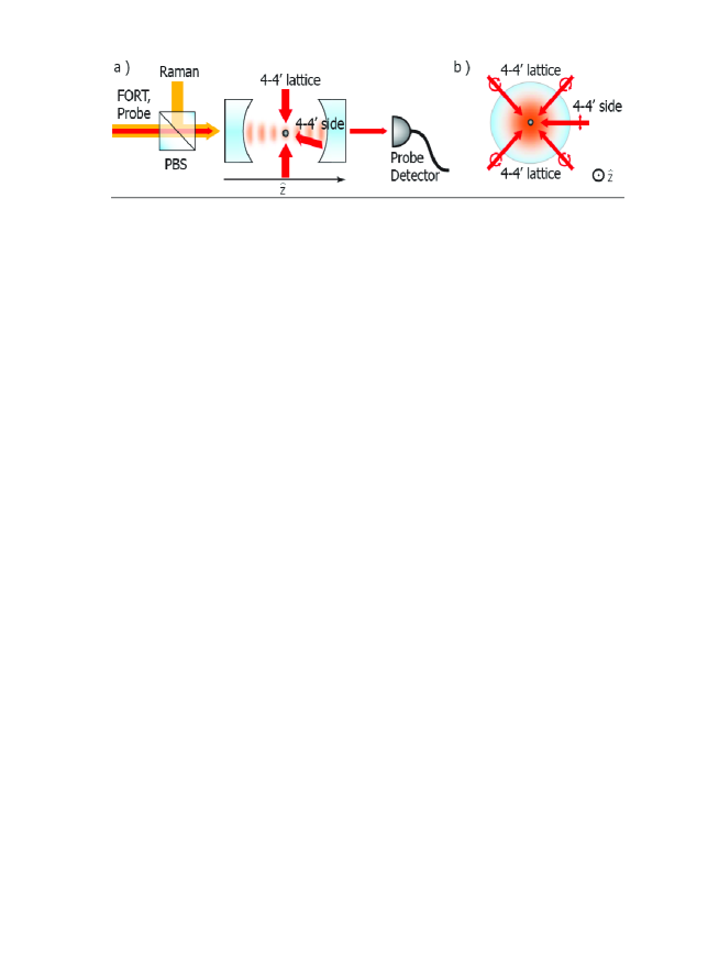
Figure 1: Schematic of experiment. (a) View from the side of the cavity. Shown are the linearly polarized FORT, Raman, and probe beams that drive the cavity, and the circularly polarized $4-4^{\prime}$ lattice beams and linearly polarized $4-4^{\prime}$ side beam that drive the atom. (b) View along the cavity axis. Shown are the $4-4^{\prime}$ lattice beams and the $4-4^{\prime}$ side beam.

The strong atom-cavity coupling allows us to to determine whether the atom is in the $F=3$ or $F=4$ hyperfine manifold by driving the cavity with a $100\,\mathrm{\mu s}$ pulse of resonant $4-5^{\prime}$ probe light, as described in Boozer06 . If the atom is in $F=4$, it couples to the cavity and blocks the transmission of the probe beam, while if the atom is in $F=3$, it decouples from the cavity, and the probe beam is transmitted. Using this technique, we can determine the hyperfine ground state of the atom with an accuracy of $\sim 98\%$ for a single $100\,\mathrm{\mu s}$ measurement interval.

Atoms are delivered to the cavity by releasing a magneto-optical trap located a few millimeters above the cavity, and the falling atoms are loaded into the FORT by cooling them with $4-4^{\prime}$ lattice light. This lattice light consists of two pairs of counter-propagating beams in the $\sigma_{+}-\sigma_{-}$ configuration, which are applied from the sides of the cavity. We ensure that only one atom is trapped in the FORT by applying the Raman beam and driving the cavity with a resonant $4-5^{\prime}$ probe; this combination gives an effect analogous to that in McKeever04 , which allows us to determine the number of atoms in the cavity based on the amount of $4-5^{\prime}$ light that is transmitted.

III Coherent and Incoherent Raman transitions

If the FORT and Raman beams are both monochromatic, then they drive coherent Raman transitions between pairs of Zeeman states $|3,m\rangle\leftrightarrow|4,m\rangle$, and the atomic populations oscillate between the two states in each pair. The effective Rabi frequency for the $|3,m\rangle\leftrightarrow|4,m\rangle$ transition is

$$\Omega_{E}(|3,m\rangle\leftrightarrow|4,m\rangle)=\Omega_{0}\,(1-m^{2}/16)^{1/2},$$ (3)

where $\Omega_{0}$ is set by the power in the FORT and Raman beams Boozer-thesis . For the experiments described here, the powers in these beams are chosen such that that $\Omega_{0}\simeq(2\pi)(120\,\mathrm{kHz})$. The Raman detuning for the FORT-Raman pair is given by $\delta_{R}=\omega_{F}-\omega_{R}-\Delta_{HF}$, where $\omega_{F}$ and $\omega_{R}$ are the optical frequencies of the FORT and Raman beams, which means that the effective detuning for the $|3,m\rangle\leftrightarrow|4,m\rangle$ transition is

$$\delta_{E}(|3,m\rangle\leftrightarrow|4,m\rangle)=\delta_{R}-\omega_{B}\,m.$$ (4)

We can also drive incoherent Raman transitions by using a monochromatic FORT beam and a spectrally broad Raman beam, where the spectral width is typically $\sim 10\,\mathrm{MHz}$. In contrast to coherent Raman transitions, in which the atom undergoes coherent Rabi oscillations, for incoherent Raman transitions the atomic population decays at a constant rate from $|3,m\rangle\rightarrow|4,m\rangle$ and from $|4,m\rangle\rightarrow|3,m\rangle$. In appendix A, we show that these decay rates are proportional to $S(\Delta_{HF}+\omega_{B}\,m)$, where $S(\omega)$ is the power spectrum of a beat note formed between the FORT and Raman beams.

IV Measuring the population distribution

Given an initial state of the atom in which the entire population lies in the $F=3$ manifold, we can use coherent Raman transitions to determine how the population is distributed among the various Zeeman states. To perform this measurement we prepare the atom in the desired initial state, apply a coherent Raman pulse of fixed duration, Rabi frequency, and Raman detuning, and then drive the cavity with a resonant $F=4\rightarrow F=5^{\prime}$ probe beam to determine if the atom was transfered to $F=4$. By iterating this process we determine the probability $p_{4}$ for the atom to be transfered by the Raman pulse, and by repeating the probability measurement for different Raman detunings $\delta_{R}$ we can map out a Raman spectrum $p_{4}(\delta_{R})$. For the Raman spectra presented here, the Raman pulses have Rabi frequency $\Omega_{0}=(2\pi)(120\,\mathrm{kHz})$ and duration $25\,\mathrm{\mu s}$. This is long enough that the Rabi oscillations decohere, and the Raman spectrum just records the Lorentzian envelope for each Zeeman transition. Thus, when the $|3,m\rangle\leftrightarrow|4,m\rangle$ Zeeman transition is resonantly driven by the Raman pulse, roughly half the population that was initially in $|3,m\rangle$ is transfered to $|4,m\rangle$.

As a demonstration of this technique, Figure 2 shows a Raman spectrum for an initial state with comparable populations in all of the $F=3$ Zeeman states. To prepare this state, we optically pump the atom to $F=3$ by alternating $7$ pulses of resonant $F=4\rightarrow F=4^{\prime}$ lattice light with $7$ pulses of resonant $F=4\rightarrow F=4^{\prime}$ side light, where each pulse is $300\,\mathrm{ns}$ long. The beams that deliver the lattice and side light are shown in Figure 1.

To determine the population $p_{3,m}$ in the Zeeman state $|3,m\rangle$, we fit a sum of Lorentzians, one for each Zeeman transition, to the experimental data:

$$p_{4}(\delta_{R})=p_{b}+(1/2)\sum_{m}(1+(\delta_{R}-\omega_{B}\,m)^{2}/(1-m^{2}/16)\,\Omega_{0}^{2})^{-1}\,p_{3,m},$$ (5)

where $p_{b}$ is a constant background. We fit the Zeeman state populations, the Rabi frequency $\Omega_{0}$, and the frequency $\omega_{B}$ that characterizes the strength of the axial bias field, and perform an independent measurement to determine the background probability $p_{b}=0.006$. The fitted value of $\Omega_{0}$ agrees to within $14\,\%$ with the value we would expect based on the measured optical powers in the FORT and Raman beams, and the fitted value of $\omega_{B}$ agrees to within $5\,\%$ with the value we would expect based on the known axial coil current and geometry. As a consistency check we sum the fitted populations and obtain the result $1.10\pm 0.03$, in reasonable agreement with the expected value of $1$.

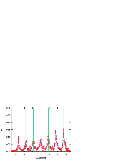
Figure 2: Raman spectrum for a random initial state. Shown is the transfer probability $p_{4}$ versus Raman detuning $\delta_{R}$: the points are the experimental data, the curve is a fit of $p_{4}(\delta_{R})$, as given by equation (5), and the vertical green lines indicate the predicted frequencies $\delta(|3,m\rangle\leftrightarrow|4,m\rangle)$ for individual Zeeman transitions.

V Optical pumping scheme

We can prepare the atom in a specific Zeeman state by using a Raman beam whose spectrum is tailored to incoherently drive all but one of the Zeeman transitions. As an example, Figure 3a shows the power spectrum of the noise used for pumping into $|3,0\rangle$. This graph was obtained by measuring the power spectrum of a beat note formed between the FORT and Raman beams by mixing them on a photodetector with a non-polarizing beam splitter. For comparison, Figure 3b shows the power spectrum for a monochromatic Raman beam tuned to Raman resonance, as would be used for driving coherent Raman transitions.

Comparing the noise spectrum shown in Figure 3a to the Raman spectrum shown in Figure 2, we see that the noise drives incoherent Raman transitions from $|3,m\rangle\leftrightarrow|4,m\rangle$ for $m\neq 0$, but because of the notch around zero detuning, the $|3,0\rangle\leftrightarrow|4,0\rangle$ transition is not driven. We optically pump the atom into $|3,0\rangle$ by first driving incoherent Raman transitions for $10\,\mathrm{\mu s}$, then pumping the atom to $F=3$ using the procedure discussed in section IV, and iterating this sequence $40$ times. It is straightforward to modify this procedure so as to pump into the $|3,m\rangle$ Zeeman state for any $m$; we simply shift the notch in the noise so that it overlaps with the $|3,m\rangle\leftrightarrow|4,m\rangle$ transition.

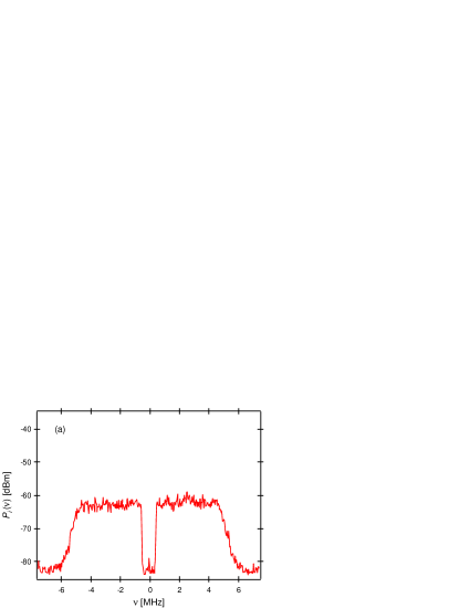
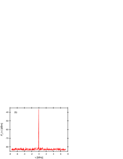
Figure 3: (a) Power spectrum of noise used for pumping into $|3,0\rangle$. (b) Power spectrum of coherent signal used for driving coherent Raman transitions with $\Omega_{0}=(2\pi)(120\,\mathrm{kHz})$. Both curves are obtained by combining the FORT and Raman beams on a photodetector and measuring the spectrum of the photocurrent; shown is the RF power in a $3\,\mathrm{kHz}$ bandwidth versus detuning from $\Delta_{HF}$.

To characterize the optical pumping, we first pump the atom into a specific Zeeman state and then measure the Raman spectrum as described in the preceding section. Figure 4 shows Raman spectra measured after pumping into (a) $|3,0\rangle$ and (b) $|3,1\rangle$. We find that the fraction of the atomic population in the desired state is $0.57\pm 0.02$ for pumping into $|3,0\rangle$ and $0.57\pm 0.02$ for pumping into $|3,1\rangle$, where the remaining population is roughly equally distributed among the other Zeeman states (these numbers are obtained using the by fitting equation (5) to the data, as described in section IV). Summing the fitted populations in all the Zeeman states, we obtain the value $1.02\pm 0.04$ for (a) and $1.08\pm 0.04$ for (b), in reasonable agreement with the expected value of $1$.

To generate the Raman beam used in Figure 3a, we start with an RF noise source, which produces broadband noise that is spectrally flat from DC to $\sim 10\,\mathrm{MHz}$. The noise is passed through a high-pass filter at $500\,\mathrm{kHz}$ and a low-pass filter at $5\,\mathrm{MHz}$, where both filters roll off at $60\,\mathrm{dB}$ per octave. The filtered noise is then mixed against an $85\,\mathrm{MHz}$ local oscillator, and the resulting RF signal is used to drive an acousto-optical modulator (AOM) that modulates a coherent beam from the injection-locked Raman laser. The first order diffracted beam from the AOM forms a Raman beam with the desired optical spectrum. Note that previous work has demonstrated the use of both synthesized incoherent laser fields Anderson90 ; Dinse88 , such as that used here, as well as the noise intrinsic to free-running diode lasers Lathi96 ; Yabuzaki91 to resonantly probe atomic spectra.

Although the scheme presented here relies on incoherent Raman transitions, it is also possible to perform optical pumping with coherent Raman transitions. The basic principle is the same: we simultaneously drive all but one of the Zeeman transitions, only instead of using a spectrally broad Raman beam, we use six monochromatic Raman beams, where each beam is tuned so as to resonantly drive a different transition. We have implemented such a scheme, and found that it gives comparable results to the incoherent scheme described above, but there are two advantages to the incoherent scheme. First, it is simpler to generate a Raman beam with the necessary spectral properties for the incoherent scheme. Second, when coherent Raman transitions are used, the six frequency components for the Raman beam must be tuned to resonance with their respective transitions, and hence are sensitive to the value of the axial magnetic field. When incoherent Raman transitions are used, however, the same Raman beam can be used for a broad range of axial field values.

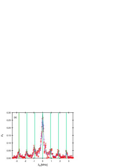
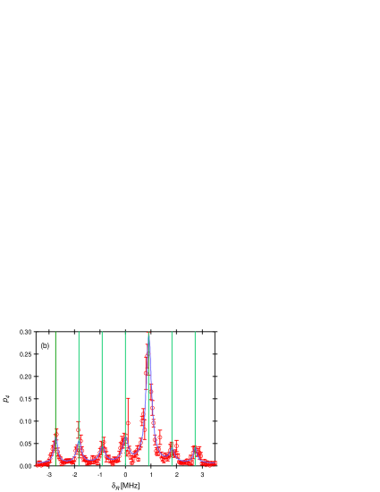
Figure 4: (a) Raman spectrum for optical pumping into $|3,0\rangle$. (b) Raman spectrum for optical pumping into $|3,1\rangle$. Raman spectrum for a random initial state. Shown is the transfer probability $p_{4}$ versus Raman detuning $\delta_{R}$: the points are the experimental data, the curve is a fit of $p_{4}(\delta_{R})$, as given by equation (5), and the vertical green lines indicate the predicted frequencies $\delta(|3,m\rangle\leftrightarrow|4,m\rangle)$ for individual Zeeman transitions.

VI Conclusion

We have proposed a new scheme for optically pumping atoms into a specific Zeeman state and have experimentally implemented the scheme with Cesium atoms in a cavity QED setting. An important advantage over existing schemes is that atoms can be prepared in any of the Zeeman states in the lower hyperfine ground state manifold.

We have measured the effectiveness of the optical pumping, and have shown that a fraction $\sim 0.57$ of the atomic population can be prepared in the desired Zeeman state. Some possible factors that could be limiting the effectiveness of the optical pumping include fluctuating magnetic fields transverse to the cavity axis, misalignment of the cavity axis with the axial bias field, and slow leaking out of the dark state due to scattering from background light. We are currently investigating these factors.

The scheme presented here operates on a fundamentally different principle from existing optical pumping schemes, in that it relies on incoherent Raman transitions to create an atomic dark state. Raman transitions have many different applications in atomic physics, so there are often independent reasons for incorporating a system for driving Raman transitions into an atomic physics laboratory; our scheme shows that such a system can also be applied to the problem of atomic state preparation. The scheme should serve as a useful tool for experiments in atomic physics, both in a cavity QED setting and beyond.

This research is supported by the National Science Foundation, the Army Research Office, and the Disruptive Technology Office of the Department of National Intelligence.

Appendix A Transition rate for incoherent Raman transitions

As described in section III, we drive incoherent Raman transitions between pairs of Zeeman states $|3,m\rangle\leftrightarrow|4,m\rangle$ by using a monochromatic FORT beam and a spectrally broad Raman beam. For incoherent Raman transitions the atomic population decays at a constant rate from $|3,m\rangle\rightarrow|4,m\rangle$ and from $|4,m\rangle\rightarrow|3,m\rangle$, and in this appendix we calculate these decay rates.

We will consider a single Zeeman transition $|3,m\rangle\leftrightarrow|4,m\rangle$, so we can treat the system as an effective two-level atom with ground state $g\equiv|3,m\rangle$ and excited state $e\equiv|4,m\rangle$, where the energy splitting between $g$ and $e$ is $\omega_{A}\equiv\Delta_{HF}+\omega_{B}\,m$. The FORT-Raman pair drives this effective two-level atom with broadband noise, which we can approximate as a comb of classical fields with optical frequencies $\omega_{k}$ and Rabi frequencies $\Omega_{k}$. Let us assume that we start in the ground state $g$. If we only consider the coupling of the atom to field $k$, then the equation of motion for the excited state amplitude $c_{e}$ is

$$i\dot{c}_{e}=\frac{\Omega_{k}}{2}\,e^{-i\delta_{k}t}\,c_{g},$$ (6)

where $\delta_{k}\equiv\omega_{k}-\omega_{A}$ is the detuning of the field from the atom. At small times the population is almost entirely in the ground state, so we can make the approximation $c_{g}=1$ and integrate equation (6) to obtain

$$c_{e}(t)=\frac{\Omega_{k}}{2\delta_{k}}(e^{-i\delta_{k}t}-1).$$ (7)

Thus, the transition rate from $g$ to $e$ for a single frequency $\omega_{k}$ is

$$\gamma_{k}=\frac{|c_{e}(t)|^{2}}{t}=\frac{\pi}{4}t\,\Omega_{k}^{2}\,D(\delta_{k}t/2),$$ (8)

where

$$D(x)\equiv\frac{\sin^{2}x}{\pi x^{2}}.$$ (9)

The total decay rate is obtained by summing the decay rates for all the fields in the comb:

$$\gamma=\sum_{k}\gamma_{k}=\frac{\pi}{4}t\sum_{k}\Omega_{k}^{2}\,D(\delta_{k}t/2).$$ (10)

To evaluate this expression we need to know the distribution of Rabi frequencies $\Omega_{k}$. This information can be obtained by forming a beat note between the FORT and Raman beams on a photodetector, and measuring the power spectrum $S(\omega)$ of the photocurrent using a spectrum analyzer. Let us first consider this measurement for a monochromatic Raman beam, and then generalize to a spectrally broad Raman beam. If both the FORT and Raman beams are monochromatic, with optical frequencies $\omega_{F}$ and $\omega_{R}$, then the resulting photocurrent $i(t)$ is given by

$$i(t)=i_{F}+i_{R}+2\eta\cos((\omega_{F}-\omega_{R})t)\,\sqrt{i_{F}i_{R}},$$ (11)

where $i_{F}$ and $i_{R}$ are the cycle-averaged photocurrents for the FORT and Raman beams taken individually and $\eta$ is the heterodyne efficiency. Thus, the power spectrum of the photocurrent has a spike at the difference frequency $\Delta\equiv\omega_{F}-\omega_{R}$:

$$S_{c}(\omega)=P_{c}\,\delta(\omega-\Delta),$$ (12)

where the integrated power $P_{c}$ of the spike is proportional to $i_{F}i_{R}$. If the difference frequency $\Delta$ is tuned to Raman resonance ($\Delta=\omega_{A}$), then the FORT-Raman pair drives coherent Raman transitions with a Rabi frequency $\Omega_{c}$ that is proportional to $\sqrt{i_{F}i_{R}}$, so

$$\Omega_{c}^{2}=\alpha P_{c},$$ (13)

where $\alpha$ is a constant that depends on various calibration factors.

Now consider the case of a spectrally broad Raman beam, which results in a photocurrent with power spectrum $S_{i}(\omega)$. The effective Rabi frequency $\Omega_{k}$ corresponding to comb line $k$ is given by

$$\Omega_{k}^{2}=\alpha\,S_{i}(\omega_{k})\,\delta\omega,$$ (14)

where $\delta\omega$ is the frequency spacing between adjacent comb lines. Substituting this result into equation (10), and replacing the sum with an integral, we obtain

$$\gamma=\frac{\pi}{4}\alpha t\int S_{i}(\omega)\,D((\omega-\omega_{A})t/2)\,d\omega.$$ (15)

If the power spectrum near $\omega_{A}$ is flat over a bandwidth $\sim 1/t$, then we can approximate $D$ as a delta function and perform the integral:

$$\gamma=\frac{\pi}{2}\alpha\,S_{i}(\omega_{A}).$$ (16)

It is convenient to use equation (13) to eliminate the calibration factor $\alpha$:

$$\gamma=\frac{\pi}{2}\frac{S_{i}(\omega_{A})}{P_{c}}\,\Omega_{c}^{2}.$$ (17)

The spectrum analyzer trace given in Figure 3a displays the power spectrum in terms of the power $P_{i}(\nu)\simeq 2\pi B\,S_{i}(\omega)$ in a bandwidth $B=3\,\mathrm{kHz}$, so we can also write this as

$$\gamma=\frac{1}{4}\frac{P_{i}(\omega_{A}/2\pi)}{P_{c}}\frac{\Omega_{c}^{2}}{B}=\frac{1}{4}(1-m^{2}/16)\,\frac{\Omega_{0}^{2}}{B}\,\frac{P_{i}((\Delta_{HF}+\omega_{B}\,m)/2\pi)}{P_{c}},$$ (18)

where we have substituted $\Omega_{c}=(1-m^{2}/16)^{1/2}\,\Omega_{0}$ and $\omega_{A}=\Delta_{HF}+\omega_{B}\,m$.

We can calculate the time evolution of the atomic populations using rate equations. It is straightforward to show that the decay rate $e\rightarrow g$ is also given by $\gamma$, and from the rate equations one can show that the excited state population is

$$p_{e}(t)=\frac{1}{2}(1-\exp(-2\gamma t)).$$ (19)

We can calculate the decay rates for the noise spectrum shown in Figure 3. For this noise spectrum the power $P_{i}(\nu)$ has roughly the same value $\bar{P}_{i}$ at the frequencies of all the $m\neq 0$ Zeeman transitions, so we can write the decay rates for these transitions as

$$\gamma(|3,m\rangle\rightarrow|4,m\rangle)=\gamma(|4,m\rangle\rightarrow|3,m\rangle)=(1-m^{2}/16)\,\Gamma,$$ (20)

where

$$\Gamma\equiv(1/4)(\Omega_{0}^{2}/B)(\bar{P}_{i}/P_{c}).$$ (21)

From the power spectrum for the noise shown in Figure 3a we have that $\bar{P}_{i}=-63\,\mathrm{dBm}$, and from the power spectrum for the coherent signal shown in Figure 3b we have that $P_{c}=-36\,\mathrm{dBm}$, where the corresponding Rabi frequency is $\Omega_{0}=(2\pi)(120\,\mathrm{kHz})$. Substituting these values into equation (21), we obtain $\Gamma=0.084\,\mathrm{\mu s}^{-1}$.

References

- (1) T. G. Walker and W. Happer, Rev. Mod. Phys. 69, 629 (1997).
- (2) D. Budker, W. Gawlik, D. F. Kimball, S. M. Rochester, V. V. Yashchuk, and A. Weis, Rev. Mod. Phys. 74, 1153 (2002).
- (3) C. Audoin, Metrologia 29, 113 (1992).
- (4) J. I. Cirac, P. Zoller, H. J. Kimble, and H. Mabuchi, Phys. Rev. Lett. 78, 3221 (1997).
- (5) P. Zoller, et al., Eur. Phys. J. D 36, 203 (2005).
- (6) J. Laurant, K. S. Choi, H. Deng, C. W. Chou, and H. J. Kimble, quant-ph/0706.0528.
- (7) C. W. Chou, J. Laurat, H. Deng, K. S. Choi, H. de Riedmatten, D. Felinto, and H. J. Kimble, Science 316, 1316 (2007).
- (8) D. Leibfriend, R. Blatt, C. Monroe, and D. Wineland, Rev. Mod. Phys. 75, 281-324 (2003).
- (9) A. Kastler, Nobel Prize Lecture. (1966)
- (10) W. Demtroder ”Laser Spectroscopy: Basic Concepts and Instrumentation,” (Springer-Verlag, Berlin, 1982) p. 567.
- (11) W. Happer, Rev. Mod. Phys. 44, 169 (1972).
- (12) L. S. Cutler, United States Patent 4,425,653.
- (13) B. Wang, Y. Han, J. Xiao, X. Yang, C. Zhang, H. Wang, M. Xiao, and K. Peng, Phys. Rev. A 75, 051801(R) (2007).
- (14) D. J. Wineland, M. Barrett, J. Britton, J. Chiaverini, B. L. DeMarco, W. M. Itano, B. M. Jelenkovic, C. Langer, D. Leibfried, V. Meyer, T. Rosenband, and T. Schaetz, Phil. Trans. Royal Soc. London A 361, 1349-1361 (2003).
- (15) C. Monroe, D.M. Meekhof, B.E. King, S.R. Jefferts, W.M. Itano, D.J. Wineland and P. Gould, Phys. Rev. Lett. 75, 4011-4014 (1995).
- (16) S. E. Hamann, D. L. Haycock, G. Klose, P. H. Pax, I. H. Deutsch, and P. S. Jessen, Phys. Rev. Lett. 80, 4149-4152 (1998).
- (17) V. Vuletic, C. Chin, A.J. Kerman, and S. Chu, Phys. Rev. Lett. 81, 5768-5771 (1998).
- (18) A. D. Boozer, A. Boca, R. Miller, T. E. Northup, and H. J. Kimble, Phys. Rev. Lett. 97, 083602 (2006).
- (19) P. Clade, E. de Mirandes, M. Cadoret, S. Guellati-Khelifa, C. Schwob, F. Nez, L. Julien, and F. Biraben, Phys. Rev. Lett. 96, 033001 (2006).
- (20) T.L. Gustavson, P. Bouyer, and M.A. Kasevich, Phys. Rev. Lett 78, 2046-2049 (1997).
- (21) I. Dotesenko, W. Alot, S. Kuhr, D. Schrader, M. Muller, Y. Miroshnychenko, V. Gomer, A. Rauschenbeautel, D. Meschede, Appl. Phys. B. 78, 711-717 (2004).
- (22) K. M. Birnbaum, Ph.D. thesis, California Institute of Technology, 2005.
- (23) T. Wilk, S. C. Webster, H. P. Specht, G. Rempe, and A. Kuhn, Phys. Rev. Lett. 98, 063601 (2007).
- (24) A. S. Parkins, P. Marte, P. Zoller, and H. J. Kimble, Phys. Rev. Lett. 71, 3095 (1993).
- (25) T. Wilk, S. C. Webster, A. Kuhn, and G. Rempe, Science 317, 488 (2007).
- (26) R. Miller, T. E. Northup, K. M. Birnbaum, A. Boca, A. D. Boozer and H. J. Kimble, J. Phys. B 38, S551 (2005).
- (27) J. McKeever, J. R. Buck, A. D. Boozer, A. Kuzmich, H.-C. Nägerl, D. M. Stamper-Kurn, and H. J. Kimble, Phys. Rev. Lett. 90, 133602 (2003).
- (28) A. D. Boozer, Ph.D. thesis, California Institute of Technology, 2005.
- (29) J. McKeever, J. R. Buck, A. D. Boozer, and H. J. Kimble, Phys. Rev. Lett. 93, 143601 (2004).
- (30) A. Boca, R. Miller, K. M. Birnbaum, A. D. Boozer, J. McKeever, H. J. Kimble, Phys. Rev. Lett. 93, 233603 (2004).
- (31) M. H. Anderson, R. D. Jones, J. Cooper, S. J. Smith, D. S. Elliott, H. Ritsch and P. Zoller, Phys. Rev. Lett. 64, 1346 (1990).
- (32) K. P. Dinse, M. P. Winters, and J. L. Hall, JOSA B 5, 1825 (1988).
- (33) S. Lathi, S. Kasapi, and Y. Yamamoto, Optics Lett. 21, 1600 (1996).
- (34) T. Yabuzaki, T. Mitsui, and U. Tanaka, Phys. Rev. Lett 67, 2453 (1991).