Acoustic phonon transport through a double-bend quantum waveguide

Abstract

In this work, using the scattering matrix method, we have investigated the transmission coefficients and the thermal conductivity in a double-bend waveguide structure. The transmission coefficients show strong resonances due to the scattering in the midsection of a double-bend structure; the positions and the widths of the resonance peaks are determined by the dimensions of the midsection of the structure. And the scattering in the double-bend structure makes the thermal conductivity decreases with the increasing of the temperature first, then increases after reaches a minimum. Furthermore, the investigations of the multiple double-bend structures indicate that the first additional double-bend structure suppresses the transmission coefficient and the frequency gap formed; and the additional double-bend structures determine the numbers of the resonance peaks at the frequency just above the gap region. These results could be useful for the design of phonon devices.

, , ,

1 Introduction

Since the discovery of the quantized electronic conductance phenomena [1, 2], the double-bend electron waveguide has been investigated as a very important case. The problem was firstly studied by Weisshaar et al. [3] using mode-matching technique. The experiment work on the low temperature conductance of the double-bend waveguide was carried out by Wu et al. [4] By using the recursive Greens function technique, Kawamura et al. [5, 6] studied this double-bend waveguide again. All the works showed strong resonant transmission due to internal reflections in the special structure and Refs. [5, 6] showed the “existence of an energy gap between the first and second subband threshold energies where the conductance is suppressed for multiple double-bend structures”. Based on the property of the strong resonant transmission through the double-bend waveguide, Shi et al. [7] proposed a simple spin filter with which an extremely large spin current is expected.

Same as the electronic conductance, the thermal conductivity is also important for semiconductor nanostructures. For an ideal elastic beam at an enough low temperature, the thermal conductivity is dominated by the ballistic phonon and is quantized in a universal unit, $\pi^{2}k_{B}^{2}T/3h$, analogous to the well-known $2e^{2}/h$ electronic conductance quantum. [8, 9, 10] These predictions have been verified experimentally [11]. Since then, many works have been done to study the geometrical effects on the transmission of the acoustic phonon and the thermal conductivity through the quantum waveguide with various geometries [12, 13, 14, 15, 16, 17, 18, 19, 20]. But as an important case, the quantum waveguide with a double-bend structure has not been studied on the phonon transmission coefficients and thermal conductivity. Therefore, in this work, we calculate the phonon transmission coefficients and thermal conductivity in a double-bend quantum waveguide using the scattering-matrix method [21, 22, 23, 24, 25] and considering the stress-free boundary condition [15, 16, 17, 18, 19, 20].

The organization of this paper is as follows. In section 2, we present the model and the numerical method briefly. The numerical results for a one double-bend structure are discussed in section 3. In section 4, the results of a two double-bend structures are presented. Finally, a summary is made in section 5.

2 Model and formalism

Figure 1: (a) Double-bend waveguide with lead width $W$, lateral length $L$, and longitudinal length $D_{1}$. (b) Two double-bend waveguides in a series with the longitudinal length $D_{2}$.

The geometry of the double-bend quantum waveguide is sketched in figure 1. Regions-I and -III are the leads of the device; region-II is the midsection. The parameters of this device are $W,L$ and $D_{1}$, which are the lateral width of the leads, the lateral width of the midsection and the longitudinal length of the midsection, respectively. We assume that the temperature in the two leads (regions-I and -III) are $T_{1}$ and $T_{2}$; and the temperature difference $\delta T$ ($\delta T=T1-T2>0$) between two leads is very small. The mean temperature $T$ ($=(T_{1}+T_{2})/2$) may then be adopted as the temperature of two leads. In this work, we choose the same thickness for the three regions and let the thickness smaller than the other two dimensions and also than the wavelength or the coherence length of the elastic waves; there is no mixing of the $z$ modes and a two-dimensional calculation is then adequate [8, 9, 10, 15]. For the imperfect contact at the regions-I and -III, the thermal conductance $K$ at temperature $T$ is given by [8, 15]

$$K=\frac{\hbar^{2}}{k_{\mathrm{B}}T^{2}}\sum_{m}\frac{1}{2\pi}\int_{\omega_{m}}^{\infty}{\tau_{m}\left(\omega\right)\frac{\omega^{2}\e^{\beta\hbar\omega}}{\left(\e^{\beta\hbar\omega}-1\right)^{2}}\d\omega},$$ (1)

where $\tau_{m}\left(\omega\right)$ is the transmission coefficient from mode $m$ of region-I at frequency $\omega$ across all the interfaces into the modes of region-III; $\omega_{m}$ is the cutoff frequency of the $m$th mode; $\beta=1/\left(k_{\mathrm{B}}T\right)$, $k_{\mathrm{B}}$ is the Boltzmann constant, $T$ is the temperature; and $\hbar$ is the Plank’s constant. It can be seen from Eq. (1) that the central issue of the problem is to obtain the transmission coefficient, $\tau_{m}\left(\omega\right)$.

We consider the scalar model for the elastic wave; the model for thin geometry at low temperature is used so that the calculation is two-dimensional. Here, we treat the simplest case for a horizontally polarized wave (SH) (polarized along the $z$ direction) propagating in the $x$-direction. So the wave equation of the displacement field $u$ is

$$\frac{\partial^{2}u}{\partial t^{2}}-v_{\mathrm{SH}}^{2}\nabla^{2}u=0,$$ (2)

where $v_{\mathrm{SH}}$ is related to the mass density $\rho$ and elastic stiffness constant $C_{44}$ by

$$v_{\mathrm{SH}}=\sqrt{C_{44}/\rho}.$$ (3)

The stress-free boundary conditions at the edges require $\hat{n}\cdot\nabla{u}=0$, where $\hat{n}$ is the unit vector normal to the edge. For the double-bend structure depicted in Fig. 1, the solution to Eq. (2) in region-$\xi$ (regions I, II and III) can be expressed as

$$u^{\xi}\left(x,y\right)=\sum_{m=0}^{N}\left[A_{m}^{\xi}\e^{\mathrm{i}k_{m}^{\xi}\left(x-x_{\xi}\right)}+B_{m}^{\xi}\e^{-\mathrm{i}k_{m}^{\xi}\left(x-x_{\xi}\right)}\right]\phi_{m}^{\xi}\left(y\right),$$ (4)

where $x_{\xi}$ is the reference coordinate along the $x$-direction in region-$\xi$; $k_{m}^{\xi}$ is the wavenumber of the transmitted and reflected waves in region-$\xi$, giving by the energy conservation condition

$$\omega^{2}={k_{m}^{\xi}}^{2}{v_{\mathrm{SH}}^{\xi}}^{2}+{m^{2}{\pi}^{2}{v_{\mathrm{SH}}^{\xi}}^{2}}/{W_{\xi}^{2}},$$ (5)

with $W_{\xi}$ the transverse dimension of region-$\xi$; $\phi_{m}^{\xi}\left(y\right)$ represents the transverse wavefunction of acoustic mode-$m$ in region-$\xi$,

$$\phi_{m}^{\mathrm{I}} = \left\{\begin{array}[]{ll}\sqrt{\frac{2}{W}}\cos{\frac{m\pi}{W}y}&\left(m\neq 0\right),\\ \sqrt{\frac{1}{W}}&\left(m=0\right);\end{array}\right.$$ (8)

$$\phi_{m}^{\mathrm{II}} = \left\{\begin{array}[]{ll}\sqrt{\frac{2}{L}}\cos{\frac{m\pi}{L}y}&\left(m\neq 0\right),\\ \sqrt{\frac{1}{L}}&\left(m=0\right);\end{array}\right.$$ (11)

$$\phi_{m}^{\mathrm{III}} = \left\{\begin{array}[]{ll}\sqrt{\frac{2}{W}}\cos{\frac{m\pi}{W}\left(y-L\right)}&\left(m\neq 0\right),\\ \sqrt{\frac{1}{W}}&\left(m=0\right).\end{array}\right.$$ (14)

In principle, the sum over $m$ in Eq. (4) includes all propagating modes and evanescent modes (imaginary $k_{m}^{\xi}$). However, in the practical calculation, besides all the propagating modes we only take a same limited number of evanescent modes into account to meet the desired precision for each region in a double-bend structure. The boundary matching conditions require the continuity of the displacement $u$ and the stress $C_{44}\partial{u}/\partial{x}$ at the interface of regions-I and -II and the interface of regions-II and -III. So we can obtain the equations for the coefficients in Eq. (4). Rewriting the resulted equations in the form of matrix, we can derive the transmission coefficient, $\tau_{m}$, by the scattering matrix method [21, 22, 23, 24, 25].

In the calculations, we employ the following values of elastic stiffness constant and the mass density [26]: $C_{44}(\mathrm{GaAs})=5.99(10^{10}\mathrm{N}\mathrm{m}^{-2})$ and $\rho(\mathrm{GaAs})=5317.6(\mathrm{kg}\mathrm{m}^{-3})$, and choosing $W=10$ nm.

3 Numerical results for a one double-bend structure

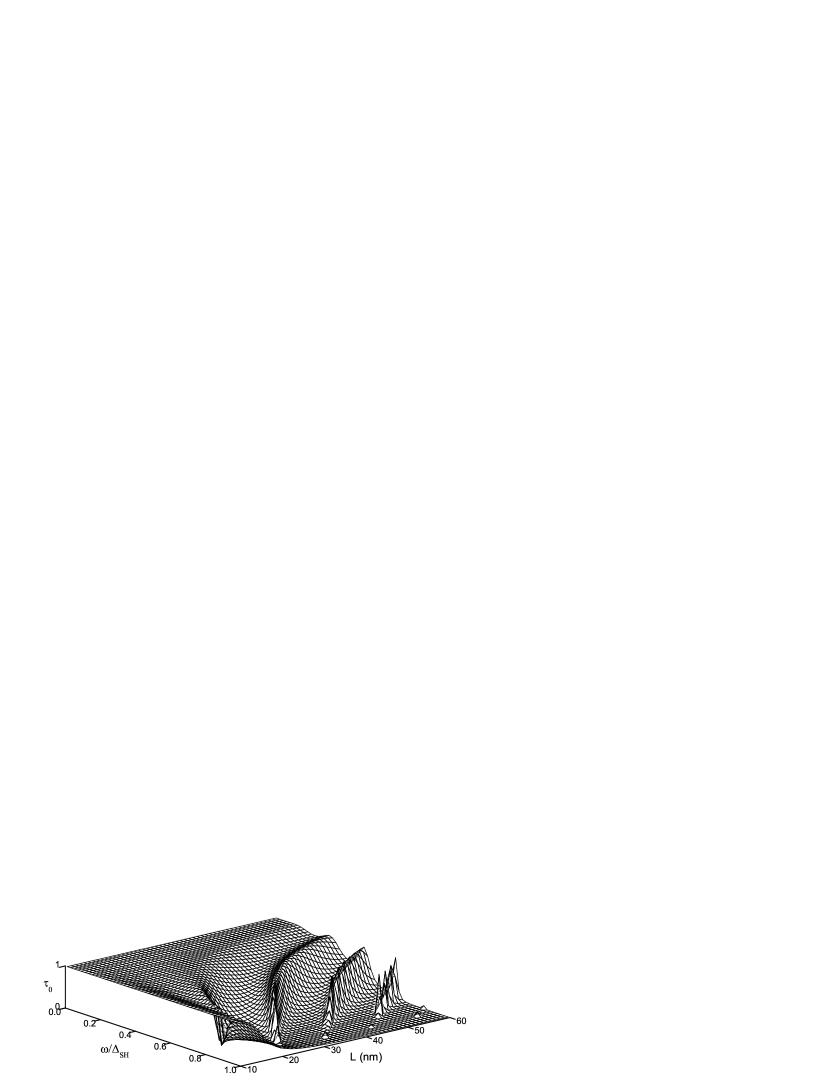
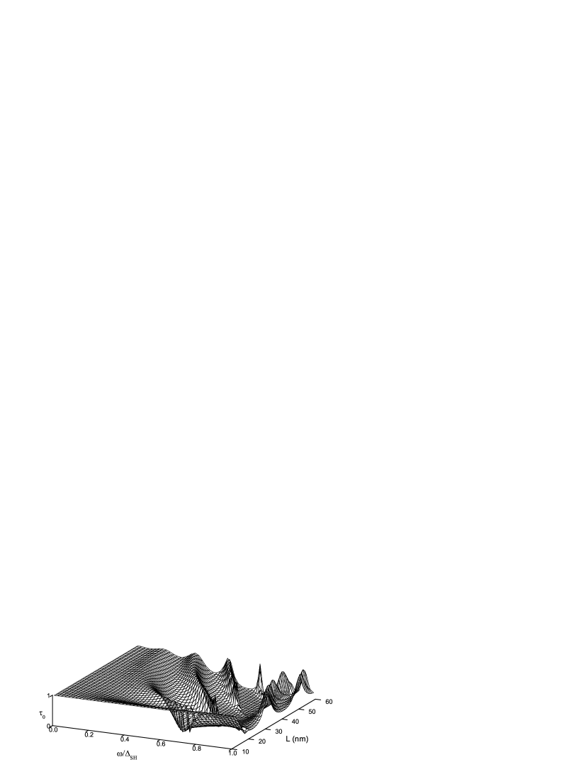
Figure 2: Transmission coefficient versus the lateral length $L$ and the incident phonon frequency $\omega/\Delta_{\mathrm{SH}}$ for the double-bend structure with $W=10$ nm, where $\Delta_{\mathrm{SH}}=\omega_{m+1}-\omega_{m}=\pi v_{\mathrm{SH}}/W$ ($v_{\mathrm{SH}}$ is the acoustic wave velocity in GaAs) represents the splitting of the cutoff frequency between the $(m+1)$th and $m$th mode in the region-I. (a) $D_{1}=10$ nm; (b) $D_{1}=12$ nm.

For acoustic phonon mode, the stress-free boundary condition allows acoustic waves propagate through the structure in the zero-th mode with cutoff frequency $\omega=0$. First, we discuss the lowest SH acoustic mode propagate through the double-bend structure shown in Fig. 1(a) from region-I to region-III. The transmission coefficients of the zero-th mode versus the lateral length $L$ and the incident phonon frequency $\omega/\Delta_{\mathrm{SH}}$ for the double-bend structure with $W=10$ nm are shown in Figs. 2 ($D_{1}=10$ nm) and 2 ($D_{1}=12$ nm). One can find from Fig. 2 that the transmission coefficient approaches unity as $\omega\rightarrow 0$ and is independent of the lateral length $L$. This is because, at $\omega\rightarrow 0$, the wavelength of the phonon is much larger than the dimension of the lateral length $L$ of region-II and the displacement field $u$ then becomes essentially the same throughout. We can also find from Fig. 2 that, for $L=10$ nm, the transmission coefficient is unity for any incident frequency. In this case the double-bend waveguide reverts to be a uniform waveguide; and in the uniform waveguide, the transmission coefficient of the zero-th mode of phonon is unity. Furthermore, from Fig. 2 one can find more resonance like features occur in the transmission coefficient with increasing incident frequency or the lateral length of region-II, $L$; and the influence of the longitudinal width $D_{1}$ also appear.

To clearly see the resonance structure in the transmission coefficient, the transmission coefficient as a function of $\omega/\Delta_{\mathrm{SH}}$ for different lateral lengths of region-II, $L$, and as a function of $L$ for different $\omega/\Delta_{\mathrm{SH}}$ are shown in Fig. 3.

In region-II, the propagation wave and reflected wave with the same wavenumber, $k=\sqrt{\omega^{2}/v^{2}-m^{2}\pi^{2}/{D_{1}}^{2}}$, will couple together. The reflected wave from region-II will interfere with the propagation wave in region-I. When the phase shift between the incident wave in the region-I and the reflected wave from the region-II reaches $2n\pi$, the transmission will be enforced, and, $\tau_{0}=1$. For a fixed lateral length $L$, same as the resonant transmission of electrons [27], the resonance condition is approximately $2k_{n}L=2n\pi$. In Figs. 3 and 3, the arrows mark the resonance positions. In Fig. 3, when $\omega/\Delta_{\mathrm{SH}}^{L}<1$, the resonance peak positions are similar as the positions in Fig. 3. This is easy to understand: in this case only the zero-th mode can exist in region-II, so the wavenumber $k=\omega/v$ is irrelevant with $D_{1}$. But for $\omega/\Delta_{\mathrm{SH}}^{L}\geq 1$, because of more than one transverse mode existing in the region-II the transmission coefficients in Fig. 3 are totally different with those in Fig. 3. Furthermore, from Figs. 3 and 3, one can find that the closer the frequency to the cutoff frequency of the $1$th mode in region-II, the narrower the resonance peak is. This is due to the fact that at the cutoff frequency of the $1$th mode, the $1$th mode is excited and the resonant condition is destroyed totally. The transmission coefficients as a function of the lateral length $L$ show periodic resonance in Figs. 3 and 3. The period is determined by the condition $2k\Delta L=2\pi$ as, $\Delta L=\pi/k=\lambda/2$. These results could be useful for the design of phonon devices.

From the transmission coefficients the thermal conductivity can be obtained from Eq. (1). Let $\omega=\eta\Delta_{\mathrm{SH}}$, $T=\zeta\Delta_{\mathrm{SH}}\hbar/k_{\mathrm{B}}$ and choose $\hbar=1$ in Eq. (1), then

$$\frac{K}{G_{q}}=\sum_{m}\int_{\eta_{m}}^{\infty}\frac{3\eta^{2}\tau_{m}\left(\eta\right)}{\pi^{2}\zeta^{3}}\frac{\mathrm{e}^{\eta/\zeta}}{\left(\mathrm{e}^{\eta/\zeta}-1\right)^{2}}\,\mathrm{d}\eta,$$ (15)

where $G_{q}=\pi^{2}k_{\mathrm{B}}^{2}T/3h$ is the universal value of the thermal conductivity. Let’s consider the integration in above equation: if $m=10$ and $\zeta\leq 1$, then $\eta_{m}=10$, $\mathrm{e}^{\eta/\zeta}\geq\mathrm{e}^{10}\gg 1$, and

Figure 3: Transmission coefficient as a function of: (a) the reduced frequency $\omega/\Delta_{\mathrm{SH}}$ with $W=10$ nm and $D_{1}=10$ nm; (b) the reduced frequency $\omega/\Delta_{\mathrm{SH}}$ and $\omega/\Delta_{\mathrm{SH}}^{L}$ with $W=10$ nm and $D_{1}=12$ nm, where $\omega/\Delta_{\mathrm{SH}}^{L}=\pi v_{\mathrm{SH}}/D_{1}$. Curves are vertically offset by $1.5$ units for clarity. The arrows indicate the resonance peaks. Transmission coefficient as a function of the lateral length $L$ with: (c) $D_{1}=10$ nm; (d) $D_{1}=12$ nm. The dotted, dashed and solid curves in (c) and (d) correspond to $\omega/\Delta_{\mathrm{SH}}=0.2$, $0.5$ and $0.8$, respectively; and in (d), these curves correspond to $\omega/\Delta_{\mathrm{SH}}^{L}=0.24$, $0.6$ and $0.96$, respectively.

$$\int_{\eta_{10}}^{\infty}\frac{3\eta^{2}\tau_{10}\left(\eta\right)}{\pi^{2}\zeta^{3}}\frac{\mathrm{e}^{\eta/\zeta}}{\left(\mathrm{e}^{\eta/\zeta}-1\right)^{2}}\,\mathrm{d}\eta$$

$$\sim\int_{10}^{\infty}\frac{3\eta^{2}\tau_{10}\left(\eta\right)}{\pi^{2}\zeta^{3}}\frac{1}{\mathrm{e}^{\eta/\zeta}}\,\mathrm{d}\eta\leq\int_{10}^{\infty}\frac{3\eta^{2}}{\pi^{2}\zeta^{3}}\frac{1}{\mathrm{e}^{\eta/\zeta}}\,\mathrm{d}\eta\leq\int_{10}^{\infty}\frac{3x^{2}}{\pi^{2}}\frac{1}{\mathrm{e}^{x}}\,\mathrm{d}x$$

$$=\frac{3}{\mathrm{e}^{10}\pi^{2}}\int_{0}^{\infty}\frac{y^{2}+20y+100}{\mathrm{e}^{y}}\,\mathrm{d}y=\frac{366}{\mathrm{e}^{10}\pi^{2}}\approx 0.00168,\qquad(\zeta\leq 1),\qquad$$ (16)

in which we have used the equation,

$$\int_{0}^{\infty}\mathrm{e}^{-sx}x^{n}\mathrm{d}x=\frac{n!}{s^{n+1}},\qquad\qquad n=0,1,2,\cdots,\quad s>0.$$ (17)

Therefore, the sum of $m$ in Eq. (1) can truncated at $m=9$ for $\zeta\leq 1$.

Figure 4: Thermal conductivity reduced by $G_{q}$, as a function of the reduced temperature, $\zeta=k_{\mathrm{B}}T/\hbar\Delta_{\mathrm{SH}}$, for the different lateral lengths of $L$: (a) the total thermal conductivity; (b), (c) and (d) are the thermal conductivity of the modes-0, 1 and 2, respectively.

Figure 5: Transmission coefficient as a function of the reduced frequency $\omega/\Delta_{\mathrm{SH}}$. (a), (b) and (c) are for $\tau_{0}$, $\tau_{1}$ and $\tau_{2}$, respectively.

Fig. 4 shows the reduced thermal conductivity $K/G_{q}$ as a function of the reduced temperature $k_{\mathrm{B}}T/\hbar\Delta_{\mathrm{SH}}$. One can find from Fig. 4(a) that the total reduced thermal conductivity approaches to the unity (i.e. the thermal conductivity, $K/T$, approaches to the ideal universal value, $\pi^{2}k_{\mathrm{B}}^{2}/3h$) when $T\rightarrow 0$; the result is independent of the lateral length of the double-bend waveguide. This is because the wavelength of the incident phonons is much larger than the dimension of the region-II when $T\rightarrow 0$ and, thus, the scattering of phonons in the region-II is negligible. Fig. 4(a) shows a thermal conductivity plateau at $L=0$ and at low temperatures due to no scattering; and the thermal conductivity increases lineally with the temperature because the higher transverse modes are excited at higher temperatures (as shown in Figs. 4(c) and 4(d)). From Fig. 4(a), for $L\neq 0$, one can find the thermal conductivity decreases from the universal value to a minimum at low temperatures, then increases with the the temperature. This can be explained from Figs. 4(b)-4(d): With increasing temperature, the thermal conductivity of the mode-0 decreases for $L\neq 0$, so the total thermal conductivity decreases from the universal value. When the temperature further increases, the higher mode can be excited and the total thermal will increase after reach the minimum. Furthermore, Fig. 4(a) shows that the total thermal conductivity decreases with increasing the lateral length; and when $L>50$ nm, the total thermal conductivity is insensitive to further increasing of $L$.

From Fig. 5(a), one can find that the transmission coefficient of the zero-th mode, $\tau_{0}$, for $L=20$ nm is higher than that for $L=50$ and $90$ nm; and $\tau_{0}$ for $L=50$ nm is similar as for $L=90$ nm. So for the thermal conductivity of mode-0 shown in Fig. 4(b), it is higher for $L=20$ nm than for $L=50$ and $90$ nm. Fig. 5(b) shows the transmission coefficients of the $1$th mode for different lateral lengths of $L$. Here, $\tau_{1}$ for $L=90$ nm is higher than that for $L=50$ nm, so the thermal conductivity for $L=50$ nm is lower than that for $L=90$ nm in Fig. 4(c). The thermal conductivity for $L=50$ nm is higher than that for $L=20$ nm shown in Fig. 4(d), because the transmission coefficient of $2$th mode for $L=50$ nm is higher than that for $L=20$ nm in Fig. 5(c).

4 Numerical results for two double-bend structures

Figure 6: (a), (b) Transmission coefficient as a function of the reduced frequency $\omega/\Delta_{\mathrm{SH}}$ for $W=10$ nm, $L=20$ nm and $D_{1}=10$ nm. (a) A two double-bend structure for different longitudinal lengths of $D_{2}$, where curves are vertically offset by $1.5$ units for clarity. (b) A two double-bend structure and a three double-bend structure for the same value of $D_{2}$.

Fig. 6 shows the transmission coefficient through a quantum waveguide with more than one double-bend structures. Fig. 6 represents the case of a two double-bend waveguide for different longitudinal lengths of $D_{2}$. One can find from the figure that an additional double-bend structure makes the frequency gap appear; and the gap width decreases with $D_{2}$ increases. Furthermore, it is obviously that the width of resonance peak at the frequency just above the gap region decreases with $D_{2}$ increases. Fig. 6 compares the transmission coefficients through a two double-bend structures and a three double-bend structures for the same value of $D_{2}$. Adding an additional double-bend structure to the two double-bend structures doesn’t change the frequency gap width but makes an additional resonance peak appearing at the frequency above the gap region. It may draw conclusions that the first additional double-bend structure to the single double-bend structure suppresses the transmission coefficient and forms a frequency gap; and an additional resonance peak is formed at the frequency just above the gap region for each additional double-bend structures. We can easily expect that an additional double-bend structure increases the scattering of the phonons so that the thermal conductivity decreases.

5 Summary

Using the scattering matrix method, we have investigated the phonon transmission and thermal conductivity in a double-bend waveguide structure. It is observed strong resonant transmission determined by the scattering in region-II. The position and the width of the resonance peaks are determined by the longitudinal length $D_{1}$ of region-II. The thermal conductivity approaches to universe value for $T\rightarrow 0$. This is because the wavelength of the incident phonons is much larger than the dimension of the region-II when $T\rightarrow 0$; the scattering of phonons by the region-II is negligible. Due to the scattering in region-II, the thermal conductivity of mode-0 decreases with increasing temperature; and at high temperatures, more than one mode are exited and the thermal conductivity of these exited modes increases. The total thermal conductivity decreases thus to a minimum, then increases with the temperature. The transmission coefficient of a double-bend structure determines the thermal conductivity for different lateral lengths of $L$.

In this paper, the transmission coefficients and the thermal conductivity in multiple double-bend waveguide structures are also studied. The results show that the first additional double-bend structure to the single double-bend structure suppresses the transmission coefficient and forms a frequency gap; and an additional resonance peak appears at the frequency just above the gap region for each additional double-bend structure. The additional double-bend structure suppresses more the thermal conductivity.

References

- [1] B.J. van Wees, H. van Houten, C.W.J. Beenakker, J.G. Williamson, L.P. Kouwenhoven, D. van der Marel, C.T. Foxon, Phys. Rev. Lett. 60 (1988) 848.
- [2] D.A. Wharam, T.J. Thornton, R. Newbury, M. Pepper, H. Ajmed, J.E.F. Frost, D.G. Hasko, D.C. Peacock, D.A. Ritchie, G.A.C. Jones, J. Phys. C 21 (1988) L209.
- [3] A. Weisshaar, J. Lary, S. M. Goodnick, V.K. Tripathi, Appl. Phys. Lett. 55 (1989) 2114.
- [4] J.C. Wu, M.N. Wybourne, W. Yindeepol, A. Weisshaar, S.M. Goodnick, Appl. Phys. Lett. 59 (1991) 102.
- [5] T. Kawamura, J.P. Leburton, J. Appl. Phys. 73 (1993) 3577.
- [6] T. Kawamura, J.P. Leburton, Phys. Rev. B 48 (1993) 8857.
- [7] Q.W. Shi, J. Zhou, M.W. Wu, Appl. Phys. Lett. 85 (2004) 2547.
- [8] L.G.C. Rego, G. Kirczenow, Phys. Rev. Lett. 81 (1998) 232.
- [9] D.E. Angelescu, M.C. Cross, M.L. Roukes, Supperlatt. Microstruct. 23 (1998) 673.
- [10] M.P. Blencowe Phys. Rev. B 59 (1999) 4992.
- [11] K. Schwab, E.A. Henriksen, J.M. Worlock, M.L. Roukes, Nature 404 (2000) 974.
- [12] D.H. Santamore, M.C. Cross, Phys. Rev. Lett. 87 (2001) 115502.
- [13] D.H. Santamore, M.C. Cross, Phys. Rev. B 63 (2001) 184306.
- [14] G. Palasantzas, Phys. Rev. B 70 (2004) 153404.
- [15] M.C. Cross, R. Lifshitz, Phys. Rev. B 64 (2001) 085324.
- [16] S.X. Qu, M. R. Geller, Phys. Rev. B 70 (2004) 085414.
- [17] W.X. Li, K.Q. Chen, W.H. Duan, J. Wu, B.L. Gu, J. Phys. D: Appl. Phys. 36 (2003) 3027.
- [18] W.X. Li, K.Q. Chen, W.H. Duan, J. Wu, B.L. Gu, J. Phys.: Condens. Matter 16 (2004) 5049.
- [19] W.X. Li, K.Q. Chen, W.H. Duan, J. Wu, B.L. Gu, Appl. Phys. Lett. 85 (2004) 822.
- [20] W.Q. Huang, K.Q. Chen, Z. Shuai, L.L. Wang, W.Y. Hu, Phys. Lett. A 336 (2005) 245.
- [21] D.Y.K. Ko, J.C. Inkson, Phys. Rev. B 38 (1988) 9945.
- [22] H. Tamura, T. Ando, Phys. Rev. B 44 (1991) 1792.
- [23] H.Q. Xu, Phys. Rev. B 50 (1994) 8469.
- [24] D. Csontos, H.Q. Xu, J. Phys.: Condens. Matter 14 (2002) 12513.
- [25] W.D. Sheng, J. Phys.: Condens. Matter 9 (1997) 8369.
- [26] K.Q. Chen, X.H. Wang, B.Y. Gu, Phys. Rev. B 61 (2000) 12075.
- [27] G. Kirczenow, Phys. Rev. B 39 (1989) 10452.