Dynamics of Vacillating Voters

Abstract

We introduce the vacillating voter model in which each voter consults two neighbors to decide its state, and changes opinion if it disagrees with either neighbor. This irresolution leads to a global bias toward zero magnetization. In spatial dimension $d>1$, anti-coarsening arises in which the linear dimension $L$ of minority domains grows as $t^{1/(d+1)}$. One consequence is that the time to reach consensus scales exponentially with the number of voters.

The voter model L99 gives an appealing, albeit idealized, description for the opinion dynamics of a socially interacting population. In this model, each node of a graph is occupied by a voter that has one of two opinions, $\uparrow$ or $\downarrow$. The population evolves by: (i) picking a random voter; (ii) the selected voter adopts the state of a randomly-chosen neighbor; (iii) repeating these steps ad infinitum or until a finite system necessarily reaches consensus. Descriptively, each voter has no self confidence and follows one of its neighbors. With this dynamics, a voter chooses a state with a probability equal to the fraction of neighbors in that state, a feature that renders the voter model soluble in all dimensions L99 ; K02 .

In this work, we investigate a variation that we term the vacillating voter model. By vacillating, we mean that a voter very much lacks confidence in its state. In an update, if a voter happens to select a random neighbor of the same persuasion, the voter is still not convinced that this state is right. Thus the voter selects another random neighbor and adopts this state. This vacillation causes a voter to change state with a larger probability than the fraction of disagreeing neighbors, and leads to a bias toward the zero-magnetization state in which there are equal densities of voters of each type.

Figure 1: Illustration of an update for the vacillating voter on the square lattice (left and middle). For the configuration on the right, the central voter flips with probability 5/6 because out of the 6 ways of selecting two neighbors, only one choice leads to both neighbors agreeable (dashed).

Thus vacillation inhibits consensus, but due to a different mechanism than that in the prototypical Axelrod model A , the bounded compromise model W and its variants VR . For these latter models, consensus is hindered because of the absence of interaction whenever two agents become sufficiently incompatible. For vacillating voters, it is individual uncertainty that forestalls consensus. The vacillating voter model also differs from models that incorporate “contrarians” galam because voters still try to imitate their neighbors.

The update steps in the vacillating voter model are:

1. Pick a random voter.

2. The voter picks a random neighbor. If the neighbor disagrees with the voter, the voter changes state.

3. If the neighbor and the voter agree, the voter picks another random neighbor and adopts its state.

4. Repeat steps 1 and 2 ad infinitum or until consensus is reached.

For example, the probability that a vacillating voter on the square lattice flips is $0,\frac{1}{2},\frac{5}{6}$, and 1, respectively, when the number of anti-aligned neighbors is 0, 1, 2, and $\geq 3$ (Fig. 1). In contrast, for the classic voter model, the flip probability is $\frac{k}{4}$, where $k$ is the number of neighbors of the opposite opinion. We now explore the consequences of this vacillation on voter dynamics.

Consider first the mean-field limit. Here the density $x$ of $\uparrow$ voters obeys the rate equation

$$\dot{x} = -x\left[1-x^{2}\right]+(1-x)\left[1-(1-x)^{2}\right]$$ (1)

$$= x(1-x)(1-2x).$$

The first term on the right accounts for the loss of $\uparrow$ voters in which a $\uparrow$ voter is first picked (factor $x$), and then the neighborhood cannot consist of two $\uparrow$ voters (factor $1-x^{2}$). Similarly, in the second (gain) term, a $\downarrow$ voter is first picked, and then the neighborhood must contain at least one $\uparrow$ voter. The factorized form shows that there are unstable fixed points at $x=0,1$ and a stable fixed point at $x=1/2$. Thus a population is driven to the zero-magnetization state.

However, because consensus is the only absorbing state of the stochastic dynamics, a finite population ultimately reaches consensus. To characterize the evolution to this state, we first study the exit probability $\mathcal{E}_{n}$, defined as the probability that a population of $N$ voters ultimately reaches $\uparrow$ consensus when there are initially $n$ $\uparrow$ voters. Then $\mathcal{E}_{n}$ obeys the backward equation fpp

$$\mathcal{E}_{n}=w_{n\to n+1}\,\mathcal{E}_{n+1}+w_{n\to n-1}\,\mathcal{E}_{n-1}+w_{n\to n}\,\mathcal{E}_{n},$$ (2)

where $w_{n\to m}$ is the probability for the transition from the state with $n$ $\uparrow$ voters to $m$ $\uparrow$ voters in an update. This equation expresses the probability to exit from $n$ as the probability to take one step (the factors $w$) times the probability to exit from the point reached after one step. In the large-$n$ limit, we write $x=n/N$, and the transition probabilities become

$$w_{n\to n+1} = (1-x)\left[1-(1-x)^{2}\right]$$

$$w_{n\to n-1} = x(1-x^{2})$$

$$w_{n\to n} = x^{3}+(1-x)^{3}.$$

Substituting these in (2), writing $\mathcal{E}_{n\pm 1}\to\mathcal{E}(x\pm\delta x)$, and expanding to second order in $\delta x$, gives

$$\frac{3x(1-x)}{2N}\frac{\partial^{2}\mathcal{E}}{\partial x^{2}}+x(1-x)(1-2x)\frac{\partial\mathcal{E}}{\partial x}=0,$$ (3)

with solution

$$\mathcal{E}(x)=\int_{-1/2}^{x-1/2}e^{2Ny^{2}/3}\,dy\Bigg{/}\int_{-1/2}^{1/2}e^{2Ny^{2}/3}\,dy.$$ (4)

Notice that $\mathcal{E}(x)$ approaches the constant value $1/2$ for increasing $N$ (Fig. 2), reflecting the bias towards the zero-magnetization state. Almost all initial states are driven to the potential well at $x=1/2$, so that the exit probability becomes independent of the initial density of $\uparrow$ voters.

Figure 2: Exit probability $\mathcal{E}(x)$ versus the density of $\uparrow$ voters $x$ for the case $N=16$, $N=25$ and $N=100$.

Similarly, we study the time to reach consensus as a function of the initial composition of voters. Let $t_{n}$ denote the time to reach consensus (either all $\uparrow$ or all $\downarrow$) when starting with $n$ $\uparrow$ voters in a population of $N$ voters. Similar to (2), $t_{n}$ obeys the backward equation fpp

$$t_{n}=\delta t+w_{n\to n+1}\,t_{n+1}+w_{n\to n-1}\,t_{n-1}+w_{n\to n}\,t_{n},$$ (5)

where $\delta t=1/N$ is the time elapsed in an update. In the large-$n$ limit, this equation becomes

$$\frac{3x(1-x)}{2N}\frac{\partial^{2}t}{\partial x^{2}}+x(1-x)(1-2x)\frac{\partial t}{\partial x}=-1.$$ (6)

The formal solution is again elementary, but the result can no longer be expressed in closed form. The main result is that the consensus time scales as $e^{aN}$, with $a$ a constant of order 1. In contrast to the classical voter model, the global bias drives the system into a potential well that must be surmounted to reach consensus. Thus the consensus time is anomalously long.

In one dimension, a voter changes its opinion if at least one of its neighbors is in disagreement. For example, a $\uparrow$ voter flips with rate 1 if the neighborhood configurations are $\uparrow\uparrow\downarrow$, $\downarrow\uparrow\uparrow$, and $\downarrow\uparrow\downarrow$. As an amusing side-note, this dynamics is equivalent to rule 178 of the one-dimensional cellular automaton wolfram , except that this rule is implemented asynchronously in the vacillating voter model. In the framework of the Ising-Glauber model IG , the flip rate of a voter at site $i$, whose states are now represented by $\sigma_{i}=\pm 1$, is

$$w(\{\sigma\}\!\!\rightarrow\!\!\{\sigma^{\prime}\}_{i})\!=\!-\frac{\left[\sigma_{i}(\sigma_{i+1}\!+\!\sigma_{i-1})\!+\!\sigma_{i-1}\sigma_{i+1}\!-\!3\right]}{4},$$ (7)

with $\{\sigma\}$ denoting the state of all voters and $\{\sigma^{\prime}\}_{i}$ the state where the $i^{\rm th}$ voter flips. The first two terms correspond to conventional Glauber kinetics, but as mentioned parenthetically in Ref. IG , the presence of the $\sigma_{i-1}\sigma_{i+1}$ term couples the rate equation for the mean spin to 3-body terms and the model is not exactly soluble.

The mean spin, $s_{j}\equiv\langle\sigma_{j}\rangle=\sum_{\{\sigma\}}\sigma_{j}P(\{\sigma\};t)$ evolves according to

$$\frac{\partial s_{j}}{\partial t} = \sum_{\{\sigma\}}\sigma_{j}\Big{[}\sum_{i}w(\{\sigma^{\prime}\}_{i}\rightarrow\{\sigma\})\,P(\{\sigma^{\prime}\}_{i};t)$$ (8)

$$~{}~{}~{}~{}~{}~{}~{}~{}-w(\{\sigma\}\rightarrow\{\sigma^{\prime}\}_{i})\,P(\{\sigma\};t)\Big{]},$$

which reduces to, after straightforward but tedious steps,

$$\frac{\partial s_{j}}{\partial t}=\frac{1}{2}\left(s_{j+1}+s_{j-1}+\langle\sigma_{j-1}\sigma_{j}\sigma_{j+1}\rangle-3s_{j}\right).$$ (9)

In a similar spirit, the rate equation for the nearest-neighbor correlation function, $\langle\sigma_{j}\sigma_{j+1}\rangle$, is

$$\frac{\partial\langle\sigma_{j}\sigma_{j\!+\!1}\rangle}{\partial t} = \frac{1}{2}\left[\langle\sigma_{j\!-\!1}(\sigma_{j}\!+\!\sigma_{j\!+\!1})\rangle+\langle(\sigma_{j}\!+\!\sigma_{j\!+\!1})\sigma_{j\!+\!2}\rangle\right]~{}~{}~{}~{}~{}$$ (10)

$$~{}~{}~{}~{}~{}~{}~{}~{}+1-3\langle\sigma_{j}\sigma_{j+1}\rangle$$

We can simplify Eq. (10) by considering domain walls—nearest-neighbor anti-aligned voters—whose density is given by $\rho=(1-\langle\sigma_{i}\sigma_{i+1}\rangle)/2$. According to the flip rate in Eq. (7), an isolated domain wall diffuses freely, just as in the pure voter model. However, when two domain walls are adjacent, they annihilate with probability 1/3 or one hops away from the other with probability 2/3. This process is isomorphic to single-species annihilation, $A+A\to 0$, but with a reduced reaction rate compared to freely diffusing reactants because of the nearest-neighbor repulsion. The domain wall density still asymptotically decays as $t^{-1/2}$ with an amplitude that depends on the magnitude of the repulsion.

Because domain walls are widely separated at long times, the second-neighbor correlation function is

$$\langle\sigma_{j}\sigma_{j+2}\rangle = +\text{prob(0 or 2 walls between\ }j\ \text{and\ }j\!+\!2)$$

$$-\text{prob(1 wall between\ }j\ \text{and\ }j\!+\!2)$$

$$\approx 1-2\rho.$$

Using the approximation of widely separated domain walls, $\langle\sigma_{j}\sigma_{j+2}\rangle\approx\langle\sigma_{j}\sigma_{j+1}\rangle\equiv m_{2}$, and the rate equation for nearest-neighbor correlation function $m_{2}$ becomes $\frac{\partial m_{2}}{\partial t}=1-m_{2}$, with solution

$$m_{2}(t)=1+\left[m(0)^{2}-1\right]\,e^{-t}.$$ (11)

Here we chose the uncorrelated initial condition, so that $m_{2}(0)=m(0)^{2}$, where $m(0)\equiv\langle s_{j}(0)\rangle$ is the average magnetization at $t=0$.

Figure 3: Exit probability $\mathcal{E}(x)$ as a function of the initial density of $\uparrow$ voters $x$ for a one dimensional system composed of 25, 36 and 1000 voters respectively The voter model result, $\mathcal{E}(x)=x$, that follows from magnetization conservation is shown for comparison.

Let us now return to the rate equation (9) for the mean spin. For a spatially homogeneous system, $\langle s_{j}\rangle$ are all identical and the magnetization is $m\equiv\langle s_{j}\rangle$. Also, we follow Ref.  MR and decouple the 3-spin correlation function as $\langle\sigma_{j-1}\sigma_{j}\sigma_{j+1}\rangle\approx mm_{2}$. Then by averaging over all sites, the rate equation equation (9) becomes

$$\frac{\partial m}{\partial t} = \frac{1}{2}(m\,m_{2}-m)=\frac{m}{2}e^{-t}(m(0)^{2}-1)\,,$$ (12)

whose solution, for the initial condition $m(0)$, is

$$m(t) = m(0)\,e^{\frac{1}{2}(1-e^{-t})(m(0)^{2}-1)}~{}.$$ (13)

Thus we obtain a non-trivial relation between final magnetization $m(\infty)$ and $m(0)$

$$m(\infty)=m(0)\,e^{\frac{1}{2}(m(0)^{2}-1)}~{}.$$ (14)

Since the density of $\uparrow$ voters is $x=(1+m)/2$, while $m(\infty)=2\mathcal{E}(x)-1$, the exit probability $\mathcal{E}(x)$ becomes

$$\mathcal{E}(x)=\frac{1}{2}\left[(2x-1)e^{2x(x-1)}+1\right].$$ (15)

This result is in excellent agreement with our simulation results (Fig. 3). For small systems ($N=25$ and $36$), we directly measure the probability $\mathcal{E}(n)$ that the population ultimately reaches a $\uparrow$ consensus when there are initially $n$ $\uparrow$ voters and averaged over 5000 realizations of the dynamics. We also verified Eq. (15) for large systems ($N=1000$ nodes) by a different approach that avoids the need to measure $\mathcal{E}(n)$ directly by simulating until ultimate consensus. Instead, we run the dynamics up to $1000$ time steps and measure the magnetization at this time. We then average over 200 realizations of the process to obtain $m(\infty)$ and finally obtain $\mathcal{E}(x)$ from $\mathcal{E}(x)=(1+m(\infty))/2$. We again find excellent agreement with our prediction (15).

Figure 4: Double logarithmic plot of the number of $\uparrow$ voters versus time on the square lattice starting from a $4\times 4$ square of $\uparrow$ voters in a background of $\downarrow$ voters.

The vacillating voter model in greater than one dimension has the new qualitative feature that small minority domains tend to grow. This anti-coarsening is a manifestation of the bias toward the zero-magnetization state. To appreciate how this anti-coarsening arises, consider a circular two-dimensional island domain of $\uparrow$ voters of linear dimension $L$ and area $A$ in a sea of $\downarrow$ voters. For large $L$, each voter at the interface has the same local environment, so that there is no environmental bias. However, there are slightly more $\downarrow$ voters just outside the circle that $\uparrow$ voters just inside. In a time of the order of $\delta t\sim L$ each interface voter is updated once, on average, so that the island area increases by an amount $\delta A$ that is of the order of the difference in the number of $\uparrow$ and $\downarrow$ voters at the interface. Thus $\frac{\delta A}{\delta t}\sim\frac{1}{L}$, which gives $L\sim t^{1/3}$. In $d$ dimensions, this same reasoning gives $L\sim t^{1/(d+1)}$. We probed for this anti-coarsening by simulating the evolution of an initial small square domain of $\uparrow$ voters in a $\downarrow$ background in two dimensions (Fig. 4). Although such domains do not remain contiguous, the data suggest that the number, or occupied area, of $\uparrow$ voters grows as $t^{\alpha}$, with $\alpha$ around 0.73, in reasonable agreement with our expectation $\alpha=2/3$.

Figure 5: Exit probability $\mathcal{E}(x)$ as a function of the initial density of $\uparrow$ voters $x$ for a square lattice of 16, 25, 36 and 49 voters, respectively, with periodic boundary conditions.

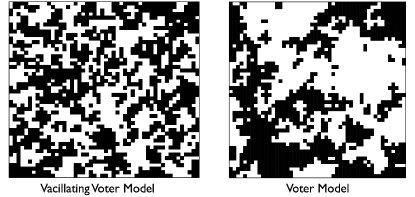
Figure 6: Snapshots of the vacillating (left) and pure (right) voter model on a $50\times 50$ lattice starting with a random zero-magnetization state after $100$ time steps. The correlation function $C_{1}$ equals $0.31$ (left) and $0.59$ (right) respectively.

A system with non-zero initial magnetization is therefore again drawn to the attractor where the density $x$ of $\uparrow$ voters equals $1/2$ before final consensus is eventually reached. It is only for $x$ initially very close to 0 or 1 that the system achieves consensus without first being drawn to this attractor. Thus the exit probability $\mathcal{E}(x)$ should be nearly independent of $x$ for almost all $x$, just as in the mean-field limit. Simulations of the vacillating voter model on the square lattice (Fig. 5) confirm that $\mathcal{E}(x)$ approaches 1/2 for a progressively wider range of $x$ as $L$ increases. Simulations also show that the correlation function $C_{1}\equiv\langle\sigma_{i,j}\sigma_{i,j+1}\rangle$ does not approach 1 in the long-time limit, as in one dimension or in the pure voter model in two dimensions. Rather, $C_{1}$ reaches the stationary value $0.31$, so that domains of opposite opinions coexist (Fig. 6), and only a rare macroscopic fluctuation allows consensus to be reached.

In summary, when vacillation is incorporated into the voter model, consensus is inhibited but not prevented. In the mean-field limit, the vacillation drives a population away from consensus and toward the zero-magnetization state. A finite system ultimately achieves consensus only via a macroscopic fluctuation that allows the system to escape this bias-induced potential well. Because of the bias, the probability to reach $\uparrow$ consensus is essentially independent of the initial composition of the population. In one dimension, the system coarsens, albeit more slowly than in the pure voter model because of the repulsion of neighboring domain walls, and the probability to reach the final state of $\uparrow$ consensus has a non-trivial initial state dependence. In two and higher dimensions, domains slowly anti-coarsen to drive the system to the zero-magnetization state. The overall behavior is qualitatively similar to that of the mean-field vacillating voter model, and very different from the pure voter model.

- (1) T. M. Liggett, Stochastic interacting systems: contact, voter, and exclusion processes, (Springer-Verlag, New York, 1999).
- (2) P. L. Krapivsky, Phys. Rev. A 45, 1067 (1992).
- (3) R. Axelrod, J. Conflict Res. 41, 203 (1977); R. Axtell, R. Axelrod, J. Epstein, and M. D. Cohen, Comput. Math. Organiz. Theory, 1, 123 (1996).
- (4) G. Weisbuch, G. Deffuant, F. Amblard, and J. P. Nadal, Complexity 7, 55 (2002); R. Hegselmann and U. Krause, J. Artificial Societies and Social Simulation 5, no. 3; E. Ben-Naim, P. L. Krapivsky, and S. Redner, Physica D 183, 190 (2003).
- (5) F. Vazquez and S. Redner, J. Phys. A 37, 8479 (2004).
- (6) S. Galam, Physica A 333 453 (2004)
- (7) See e.g., S. Redner, A Guide to First-Passage Processes, (Cambridge University Press, New York, 2001), Chap. 2.
- (8) S. Wolfram, A New Kind of Science, (Wolfram Media, Champaign, IL, 2002).
- (9) R. J. Glauber, J. Math. Phys. 4, 294 (1963).
- (10) M. Mobilia and S. Redner, Phys. Rev. E 68 046106, (2003).