A Quantitative Link Between Globular Clusters and the Stellar Halos in Elliptical Galaxies

Abstract

This paper explores the quantitative connection between globular clusters and the “diffuse” stellar population of the galaxies they are associated with. Both NGC 1399 and NGC 4486 (M87) are well suited for this kind of analysis due to their large globular cluster populations.

The main assumption of our Monte Carlo based models is that each globular cluster is formed along with a given diffuse stellar mass that shares the same spatial distribution, chemical composition and age. The main globular clusters subpopulations, that determine the observed bimodal colour distribution, are decomposed avoiding a priori parametric (e.g. Gaussian) fits and using a new colour (C-T₁)-metallicity relation. The eventual detectability of a “blue” tilt in the colour magnitude diagrams of the blue globulars subpopulation is also addressed.

A successful link between globular clusters and the stellar galaxy halo is established by assuming that the number of globular clusters per associated diffuse stellar mass t is a function of total abundance [Z/H] and behaves as $t=\gamma\exp(-\delta[Z/H])$ (i.e. increases when abundance decreases).

The simulations allow the prediction of a surface brightness profile for each galaxy through this two free parameters approximation. The $\gamma$, $\delta$ parameters that provide the best fit to the observed profiles in the B band, in turn, determine several features, namely, large scale halo colour gradients, globular clusters-halo colour offset, clusters cumulative specific frequencies, and stellar metallicity distributions, that compare well with observations.

The results suggest the coexistence of two distinct stellar populations characterised by widely different metallicities and spatial distributions. One of these populations (connected with the blue globulars) is metal poor, highly homogeneous, exhibits an extended spatial distribution and becomes more evident at large galactocentric radius contributing with some 20% of the total stellar mass. In turn, the stellar population associated with the red globulars is extremely heterogeneous and dominates the inner region of both galaxies.

Remarkably, and although the cluster populations of these galaxies exhibit detectable differences in colour distribution, the $\delta$ parameter that determines the shape of the brightness profiles of both galaxies has the same value, $\delta\approx$ 1.1 to 1.2 $\pm 0.1$.

1 Introduction

The idea that globular clusters (GCs) harbour important clues in relation with the early stages of galaxy formation is a widely accepted concept. One of the most compelling arguments in favour of the existence of a connection between GCs and major star formation episodes in the life of a galaxy is the constant cluster formation efficiency, defined in terms of total baryonic mass (McLaughlin, 1999), in different galaxies.

However, breaking the code that leads to a detailed quantitative link between GCs and the underlying “diffuse” stellar population is still an open question. Such a connection has been discussed on theoretical (e.g. Beasley et al. 2002 or, more recently, Pipino et al. 2007) and observational grounds (e.g. Forbes & Forte 2001). In the particular case of Milky Way GCs, Pritzl, Venn & Irwin (2005) found that the chemical similarities between clusters and field stars with $[Fe/H]\leq-1$ suggests a shared chemical history in a well mixed early Galaxy.

Clarifying this issue may certainly yield some arguments in favour (or against) some predominant ideas that have been widely referenced in the literature (e.g. Eggen et al. 1962; Searle & Zinn 1978) and later explored within the frame of different scenarios (e.g. Ashman & Zepf 1992, or Forbes et al. 1997).

A good perspective of the complex situation in this context is given in the thorough review by Brodie & Strader (2006) and Larson (2006).

An initial confrontation between GCs and halo stellar populations shows more differences than similarities: a) In general, GCs exhibit more shallow spatial distributions than those characterising galaxy light (e.g. Racine et al. 1978; Dirsch et al. 2003); b) There is a colour offset in the sense that mean integrated globular colours appear bluer than those of the galaxy halos at the same galactocentric radius (Strom et al. 1981; Forte, Strom & Strom 1981; Jordan et al. 2004); c) GCs show frequently bimodal colour (and hence, metallicity) distributions (see, for example, Peng et al. 2005). This feature does not seem exactly shared by the resolved stellar populations in nearby resolved galaxies (see Durrell et al. 2001; Harris & Harris 2002; Rejkuba et al. 2005 or Mouhcine 2006).

As discussed later in this work, those differences arise, mainly, from the fact that GCs analysis usually provide number weighted statistics while galaxy halos observations yield luminosity weighted measurements.

A preliminary quantitative approach to the globulars-stellar halo connection was presented in Forte, Faifer & Geisler (2005) (hereafter FFG05). This last paper shows that, given the areal density distribution of the “blue” and “red” globular cluster subpopulations in NGC 1339, the galaxy surface brightness profile, galactocentric colour gradient and cumulative GCs specific frequency, can be matched by linearly weighting the areal density profiles. The “weight” corresponding to each component of the brightness profile is the inverse of the intrinsic GCs frequency characteristic of each cluster population.

The main argument behind that approach is that the shape of the colour (and metallicity) distribution of each globular cluster subpopulation does not change with galactocentric radius. Large angular scale studies (Dirsch et al. 2003; Bassino et al. 2006) in fact show that the colour peaks in the GCs colour statistics of NGC 1399 keep the same position (or show very little variation) over large galactocentric ranges. A similar result is obtained for NGC 4486 by Kundu & Zepf (2007) who find those peaks do not show a detectable variation in colour over 75 kpc in galactocentric radius.

It must be stressed that those subpopulations are “phenomenologically” defined in terms of their integrated colours but each might eventually have a given spread in age and/or metallicity.

The presence of a “valley” in the globular colour statistics is usually adopted as a discriminating boundary between both subpopulations. The need to revise such a procedure was already suggested by figure 5 in FFG05. This last diagram showed that the NGC 1399 GCs bluer than the blue peak have a distinct behaviour of the areal density profile, exhibiting a flat core that disappears when all “blue” clusters (i.e. all GCs bluer than the colour valley) are included in the sample. That result prompted for a further analysis as discussed below.

This paper generalises the FFG05 approach trough Monte-Carlo based models. In this frame, “seed” globulars are generated following a given abundance Z distribution and then associated with a “diffuse” stellar mass that shares its age, chemical composition and statistical spatial distribution. The luminosity associated with this mass is derived from a mass to luminosity ratio adequate for a given age and metallicity. These models aim at reproducing the features mentioned above and seek for a function that could link GCs and diffuse stellar populations keeping a minimum number of free parameters.

Both NGC 1399 and NGC 4486 appear as adequate targets in order to perform such a modelling due to their prominent globular cluster systems (GCS). Although these systems show some structural similarities in terms of their spatial distribution, they also differ markedly both in the shape of their GCs colour statistics and specific frequencies (Forte et al., 2002).

This work also presents new Washington photometry, obtained and handled in a homogeneous way, that allows for a re-discussion of the GCS properties in the inner region of both galaxies and, in particular, of the behaviour of the areal density of GCs with colour. In turn, recent wide field photometric studies of the GCS associated with NGC 1399 (Bassino et al., 2006) and NGC 4486 (Tamura et al. 2006a; Tamura et al. 2006b), are well suited for extending the analysis to larger galactocentric radii.

2 Observations and data handling

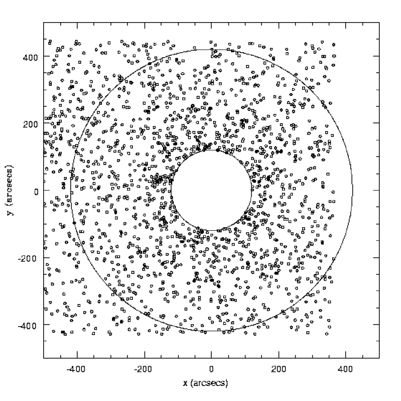
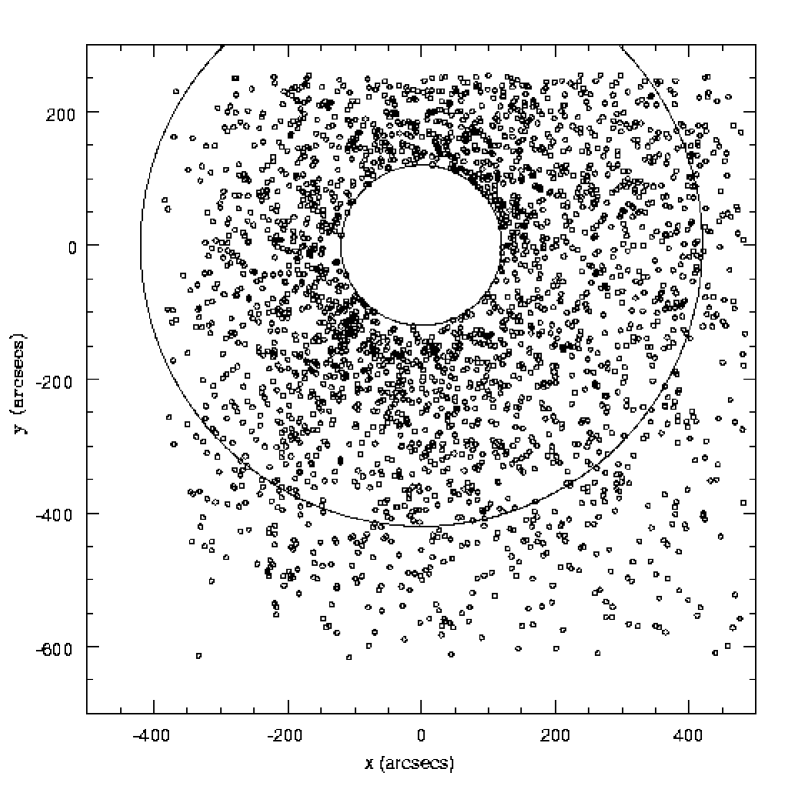
Figure 1: Distribution GCs candidates brighter than T${}_{1}=23.2$. Left panel: NGC 1399 field. North is to the right and East is up. Right panel: NGC 4486 field. North is up and East to the left. In both panels, circles have radii of 120 and 420 arcsec respectively. The GC sample completeness in these areas is close to 95%.

Photometric observations were carried out with the Mayall and Blanco 4-m telescopes at KPNO and CTIO respectively and 2048 pixels on a side CCDs, with a pixel scale of 0.43 arcsecs. The C filter from the Washington System (Harris & Canterna, 1979) and the R_KC filter of the Kron-Cousins system were used at both telescopes. As noted by Geisler (1996) this last filter is comparable to the T₁ filter in the Washington system although much more efficient in terms of transmission. In what follows we keep the T₁ denomination for our red magnitudes.

Two R_KC images (exposure: 600 secs each) and three C images (exposure: 1500 secs each) were secured for both galaxy fields.

Seeing quality for these frames varied between 1.0 and 1.6 arcsec. These images were processed with the CCDRED routines within IRAF including bias and flat fielding.

The galaxy background removal was performed with routins included in the VISTA image prossesing systems.

PSF photometry on all the frames was then carried out using the ALLFRAME version of the DAOPHOT package (Stetson 1987; Stetson 1991).

The instrumental photometry was transformed to the standard system using calibration standard stars from Geisler (1996).

Image classification, in terms of resolved and non-resolved objects, was performed as in Forte et al. (2001). Briefly, that procedure combined the use of the round and sharpness parameters defined in DAOPHOT and also the mirrored envelope of the T₁ PSF ALLFRAME magnitude vs. the difference between this magnitude and that obtained using aperture photometry for every object detected on the images.

Non-resolved objects brighter than T${}_{1}=23.2$ and with (C-T₁) colours between 0.9 and 2.3 were considered as cluster candidates and their distribution on the sky is depicted in Figure 1.

Circles with r=120 and 420 arcsec delineate the area used for the analysis of the surface density distributions in the inner regions of the galaxies.

Figure 2 shows the errors on the (C-T₁) colours as a function of T₁ magnitude as delivered by DAOPHOT. A median error for the (C-T₁) colours of $\pm$ 0.07 mags. is reached at T${}_{1}=23.2$, which is adopted in what follows as the limiting magnitude of the analysis in order to assure good quality colours.

The photometric data for both galaxies, Table 1 and 2, are available in the electronic journal version. Coordinates are referred to the galaxy centers and defined as in Figure 1

Table 1: Photometric data NGC 1399.

ID	X (arcsec)	Y (arcsec)	T1	(C-T1)	roundness
537.	196.8	-427.6	24.15	0.63	0.77
553.	136.5	-427.5	24.33	0.65	0.85

Table 2: Photometric data NGC 4486.

ID	X (arcsec)	Y (arcsec)	T1	(C-T1)	roundness
23314.	-13.1	-126.5	21.67	1.43	0.93
23406.	-32.1	-124.9	23.39	1.26	0.94

ADDSTARS experiments were carried out to estimate the completeness of the non-resolved objects (which is expected to be the case for GCs at the distances of NGC 1399 and NGC 4486 from the sun). Ten images, adding 1000 artificial stars each, on both C and T₁ master images, yielded a completeness of 94 and 96% at T${}_{1}=23.2$, for NGC 1399 and NGC 4486 respectively.

A comparison field of 77.7 arcmin${}^{\sq}$ was taken from Forte et al. (2001) who performed C and T₁ photometry following the same procedure. This field has 146 non-resolved objetcs within the colour-magnitude boundaries adopted for the globular cluster candidates.

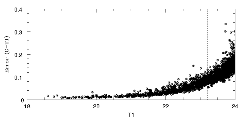
Figure 2: (C-T₁) colour errors as a function of T₁ magnitude for both galaxy fields. The vertical line at T${}_{1}=23.2$ is the limiting magnitude adopted in the analysis. The median colour error for the sample is 0.04 mags.

3 Colour-magnitude diagrams and Colour Distributions

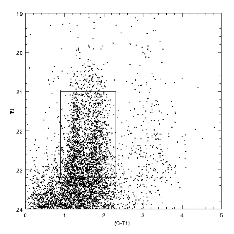
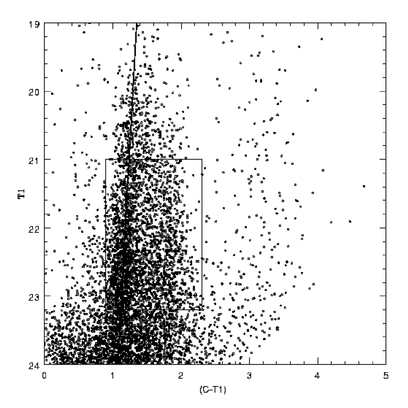
Figure 3: T₁ vs. (C-T₁) colour magnitude diagram for unresolved objects in the field of NGC 1399 (upper panel) and NGC 4486 (lower panel). The domain of the GCs candidates discussed in the text is indicated by the rectangular area. The tilted line, for NGC 4486, is defined by the modal values of the colour statistic inside 0.5 mags. intervals in T₁ for the blue GCs.

The T₁ vs. (C-T₁) colour diagrams for non-resolved objects are displayed in Figure 3. The limiting magnitude T${}_{1}=23.2$ is indicated as a horizontal line while vertical lines at (C-T₁)=0.90 and (C-T₁)=2.30 define the domain of the globular cluster candidates.

A distinctive feature in the lower panel of Figure 3, in contrast with the upper panel of the same figure, is a noticeable tilt of the colours of the blue clusters associated with NGC 4486, which is not detectable in the case of NGC 1399. The tilted line Figure 3 (lower panel) was obtained by fitting the modal values on a smoothed image of the colour magnitude diagram (adopting a round Gaussian kernel of 0.05 mags.) yielding:

$$T_{1}=41.50-16.67(C-T_{1})$$ (1)

This relation implies a 0.06 mags. (C-T₁) colour increase per magnitude that is comparable to that detectable in the (g-z) colours of 0.045 per magnitude (Strader et al., 2006). The possible reason for the presence of a “blue” tilt in the colour magnitude diagram is discussed in Section 8.

The (C-T₁) colour histograms for GCs within a circular galactocentric region defined between 120 and 360 arcsec are depicted in Figure 4. These histograms have been corrected for background contamination by subtracting the comparison field histogram (scaled by area and also shown in these figures) and contain about 1000 and 1800 candidate GCs for both galaxies, respectively.

In order to minimise the presence of bright objects that might be identified as compact dwarfs (see Phillips et al. 2001) we adopted an upper cut off at T₁=21.0. We stress that Ostrov, Forte & Geisler (1998) noted that NGC 1399 cluster candidates brighter than this magnitude exhibit a unimodal colour distribution, a feature later confirmed in Dirsch et al. (2003). As a reference we point out that Omega Cen-like objects would appear at T₁ $\approx$ 21.4 and 21.0 for NGC 1399 and NGC 4486, respectively.

These last figures also indicate the position of the so called “colour valleys” at (C-T₁)=1.55 and 1.52 for NGC 1399 and NGC 4486 respectively. These values were determined using Gaussian smoothed colour histograms with a colour kernel of 0.05 mags. The same procedure leads to (C-T₁)=1.26 and 1.21 for the blue peaks and (C-T₁)= 1.75 and 1.72 for the red peaks in both galaxies.

Figure 4: (C-T₁) background corrected colour histogram for NGC 1399 (left panel) and NGC 4486 (right panel) globular candidates within a circular annulus defined between 120 and 360 arcsec in galactocentric radius. In both cases the areal scaled subtracted background is shown by the dotted line histograms. The combined counting statistical error bars are also shown. The histograms contain $\approx 1000$ and $\approx 1800$ cluster candidates for NGC 1399 and NGC 4486, respectively. Vertical lines idicate the position of the colour valleys.

4 Description of the model

In this section we describe each of the steps involved in the model an the main hypothesis behind it, namely:

1. The decomposition of the colour histograms in terms of the cluster subpopulations leading to their [Z/H], [Fe/H] and (C-T₁) colour distributions.

2. The determination of the projected areal density distribution for each of the cluster subpopulations.

3. Establishing the link between each cluster and its associated diffuse stellar population.

4. Deriving the parameters that determine the shape of the predicted galaxy surface brightness profile.

a) The decomposition of the colour histograms.

The first step is the decomposition of the the observed colour histograms shown in Figure 4 avoiding an a priori functional dependence (e.g., the usual Gaussian assumption). It must be emphasised that, matching the two-peaked colour histograms observed both in NGC 1399 and NGC 4486 through the adopted colour-metallicity relation (see below), necessarily requires two distinct globular cluster populations.“Seed” clusters were then randomly generated in the abundance Z domain according to a given statistical dependence. Trial and error shows that exponential behaviours $f(Z)\approx\exp[-(Z-Zi)/Zs]$ where $Zs$ is the abundance scale length and $Zi$ is the minimum abundance, provides acceptable fits to the observed histograms (i.e., within the Poissonian uncertainties associated with each statistical bin). Some more complex functions cannot be rejected but would imply a larger number of free parameters not justified in terms of those uncertainties.

As for the minimum abundance, we adopted $Zi=0.003Z_{\odot}$, that corresponds to $[Fe/H]=-2.65$ in the metallicity scale presented below. As discussed later, a dependence of $Zi$ with T₁ leads to a blue tilt that reproduces the colour-magnitude diagram of the NGC 4486 GCS.

The decomposition procedure aims at matching the position of the colour peaks and colour valley while keeping a minimum value of the quality index of the fit, $\chi^{2}$ , defined as in Côté et al. (1998).

The cluster abundance $Z$ was linked to metallicity on the Zinn and West (1984) scale. The adoption of the [Fe/H]zw scale imply some caveats (see for example, Thomas et al. 2003 or Strader et al. 2007) about the nature of this index. In this work we use the relation found by Mendel, Proctor & Forbes (2007) for the stellar population models given by Thomas, Maraston & Korn (2004) :

$$[Fe/H]zw=[Z/H]-0.131$$ (2)

An integrated colour was then obtained for each cluster through an empirical (C-T₁)-[Fe/H] colour-metallicity calibration.

Several approach have been made in the past aiming at determining the colour metallicity relation. For example, the original linear relation found by Geisler & Forte (1990) for MW clusters was later improved by Harris & Harris (2002). Being an important step in the modelling process, we attempted a new calibration, described in Section 5, which yields a quadratic relationship between metallicity and integrated cluster colours.

Before comparing the model cluster colours with the observed histograms, we added interstellar reddenings, ($E(B-V)=0.015$ and $0.022$ for NGC 1399 and NGC 4486, respectively) from the Schlegel et al. (1998) maps, adopting $E(C-T_{1})=1.97E(B-V)$, and Gaussian errors matching their behaviour as a function of cluster brightness displayed in Figure 2.

Figure 5: Model fit (continuous line) to the kernel histogram representative of globular clusters associated with the brightest ellipticals (black dots) in the Virgo ACS by Peng et al. (2005). The adopted Gaussian colour kernel is 0.05 mags. The two components correspond to $Zs$ of $0.035Z_{\odot}$ and $1.05Z_{\odot}$ for the blue (dotted line) and red (dashed line) clusters subpopulations respectively with peaks at (g-z)=0.92 and 1.43 (vertical lines).

Figure 6: Upper panel: Colour histogram for 91 MW globular clusters. The bars indicate the statistical count uncertainties. The continuous line is a model fit described in text. Lower panel: Model components for MW globulars. Blue clusters are fit with an abundance scale $Zs(blue)=0.035Z_{\odot}$ and red globulars with $Zs(red)=0.50Z_{\odot}$. Colour peaks at $(C-T_{1})_{o}=1.15$ and 1.51 are indicated by vertical bars.

Examples of the decomposition procedure are shown in figures 5 and 6. The first diagram displays the results obtained from fitting the kernel colour distribution of GCs belonging to the brightest galaxies sample in the Virgo ACS (Peng et al. 2005; figure 5). These galaxies are comparable in brightness to both NGC 1399 and NGC 4486. The parameters of the best fit are $Zs(blue)=0.035Z_{\odot}$ for the blue clusters (23% of the total population) and $Zs(red)=1.05Z_{\odot}$ for the red clusters. In this case, we transformed the (C-T₁) colours to (g-z) by adopting:

$$(g-z)=(C-T_{1})-0.29$$ (3)

This colour transformation is consistent with the colour of the peaks in the ACS bright galaxies sample compared to our estimate of the (C-T₁) peaks in Figure 4 and also with the colours relation derived from the Maraston (2004) models.

Figure 6 shows the best fit obtained for 91 MW globulars with (C-T₁) colours (from Harris & Canterna 1977) or (B-I) colours (transformed according to $(C-T_{1})_{o}=1.03(B-I)_{o}-0.43$) in Reed et al. (1988). In this case, 70% are assigned to the blue clusters subpopulation, with $Zs(blue)=0.035\pm 0.01Z_{\odot}$, and the remaining 30% to the red one, with $Zs(red)=0.50\pm 0.05Z_{\odot}$. These parameters imply [Fe/H] peaks at -1.7 and -0.5, respectively. The small sample of MW clusters has large statistical uncertainties but the fit is consistent with the observed shape of the [Fe/H] distribution (see Bica et al. 2006 and references therein).

b) Projected spatial distributions.

The model assumes that each of the GCs subpopulations has its own and distinctive spatial distribution. As noted before, however, the adoption of a given colour window to define each cluster subpopulation, leads to ambiguous results in the case of NGC 1399. This particular aspect is discussed with more detail in Section 6 on the basis of the photometry presented in this paper. In particular, we stress that the variation of the slope observed for the blue GCs (depending on the colour window adopted as their domain) may arise as a partial superposition of the two cluster subpopulations.

c) The GCs-diffuse stellar population link.

Zepf & Ashman (1993) introduced the T parameter, defined as the total number of GCs per galaxy stellar mass unit. In this work, we generalise that parameter by assuming that the number of globular clusters per associated diffuse stellar mass t is a function of total abundance [Z/H]. After exploring different possible functions, we adopted: $t=\gamma\exp(-\delta[Z/H])$ (i.e. t increases when abundance decreases), and then:

$$dN/d[Z/H]=t([Z/H])M([Z/H])$$ (4)

where dN is the number of CGs associated with a stellar mass M and an abundance [Z/H] that belongs to a given subpopulation. This assumption leads to a “diffuse” stellar mass per cluster with a given [Z/H]:

$$M^{*}=1/t$$ (5)

and then to an integrated luminosity:

$$L=M^{*}/(M/L)$$ (6)

Where (M/L) is the mass-luminosity ratio characteristic for stars with the same age and metallicity of the “seed” globular cluster.

In this work we adopted the (M/L) ratio for the B (Johnson) band given by Worthey (1994) and an age of 12 Gy. This ratio can be approximated as

$$(M/L)_{B}=3.71+([Z/H]+2.0)^{2.5}$$ (7)

This approximation differs from the Worthey’s (M/L) ratios by, at most, $\approx 7\%$.

Note that we adopt [Z/H] instead of [Fe/H] as Worthey’s models assume solar scaled metallicities. A comparison with other models gives an idea about the uncertainty in this ratio. For example, models in Maraston (2004), for the same age and a Salpeter luminosity function, show an overall agreement better than $10\%$ with Worthey’s except at the lowest abundance where they deliver a ratio $\approx 24\%$ larger. The effect of age variations on this ratio is discussed below.

In particular, we choose the B and R bands since large scale surface photometry is available for both NGC 1399 and NGC 4486 (see Sections 7 and 8) and no comparable data has been published in the C and T₁ bands for both galaxies.

Although the $(M/L)_{B}$ ratio depends on age, we stress that most works (e.g. Jordan et al. 2002) have not detected significant age differences for the cluster subpopulations in NGC 4486. In turn, Forbes et al. (2001) (and also see Pierce et al. 2006a; Pierce et al. 2006b or Hempel et al. 2007) find arguments to support the presence of a fraction of “intermediate age” clusters in NGC 1399 and in other galaxies. However, age differences as large as $\pm$ 2 Gy will not have a strong impact on the integrated colours.

d) The shape and colour of the galaxy surface brightness profile.

Each stellar mass element associated with a given “seed” GC (and determined by the adopted $\gamma$ and $\delta$ parameters) was split into a number of “luminous” particles (i.e. 100 per cluster). These particles were statistically located on the plane of the sky by adopting the same spatial distribution that characterises each of the cluster subpopulations in order to construct bi-dimensional blue image (2 arcsec per pixel) of the galaxies. A red image was also obtained by transforming the (C-T₁) colour of each luminous particle to (B-R) by means of:

$$(B-R)_{KC}=0.704(C-T_{1})+0.269$$ (8)

empirically obtained from MW GCs with Johnson (Reed et al., 1988) and Washington (Harris & Canterna, 1977) photometry.

The synthetic B and R_KC images were then analysed with the task ELLIPSE within IRAF in order to derive surface brightness profiles and colour gradients along the semi-major axis of the galaxies and, in the case of NGC 4486, the variation of ellipticity along the same axis.

This treatment generalises the profile expression given in FFG05:

$$\mu_{B}=(V-Mv)_{o}+A(B)+2.5log\big{[}S_{B}(red)\big{]}$$

$$-2.5log\big{[}N(red)+\frac{N(blue)}{C_{B}}\big{]}$$ (9)

where N(blue), N(red) are the areal densities of the blue and red clusters at a given galactocentric distance and $C_{B}=S(blue)/S(red)$. Introducing the definition of the t parameter given before, leads to:

$$Sn^{-1}=\frac{1.0}{\gamma}\int_{[Z/H]_{l}}^{[Z/H]_{u}}{\frac{dn}{d[Z/H]}\frac{1.0}{(M/L)}\exp{\{\delta[Z/H]\}}d[Z/H]}$$ (10)

where the integrals are performed on the abundance domains covered by each cluster family and $dn/d[Z/H]=N^{-1}dN/d[Z/H]$, being N the projected areal density of each GCs subpopulations at a given galactocentric radius, and $dn/d[Z/H]$ comes from the histogram decomposition. Note that the Sn values do not change with galactocentric radius and are solely determined by the Z distribution parameters of each cluster and associated stellar subpopulation (which we also call “blue” and “red” in what follows).

Both $\gamma$ and $\delta$ were iteratively changed in order to derive a surface brightness profile that minimises the rms of the residuals when confronted with the observed profiles at galactocentric distances larger than 120 arcsec. This last value was adopted since both GCS exhibit flat spatial density cores that contrast with the peaked shape of the galaxy surface brightness.

These cores can be understood as the result of gravitational disruption effects that change the original population of GCs in the inner regions of galaxies (see, for example, Capuzzo-Dolcetta & Tesseri 1999, and references therein) and, presumably, become less important for cluster orbits with larger perigalactic values.

5 Colour-metallicity Calibration

We present a new colour metallicity relation based on 198 clusters that combines revised data for MW GCs and also metallicity data obtained for GCs in three other galaxies: NGC 3379, NGC 3923, and NGC 4649 (Pierce et al. 2006a; Pierce et al. 2006b, and Norris et al. 2007, in prep.). [Fe/H] values for GCs in these galaxies were derived from Lick indices given in the Thomas et al. (2004) stellar population models. Theses works were selected as they were homogeneous both in data handling and in the derivation of the Lick indices.

In the case of MW clusters, we first looked for a transformation of colours in the Johnson system to (C-T₁). A large photometric sample, that includes (B-I) colours, is available in Reed et al. (1988). In turn, (C-T₁) colours were obtained from Harris & Canterna (1977). Intrinsic colours for these globulars were then obtained by using colour excesses determined by Recio Blanco (2005), when available, or the Reed et al. (1988) values. As a result we obtain:

$$(C-T_{1})_{o}=1.03(\pm 0.02)(B-I)-0.43(\pm 0.03)$$ (11)

In turn, the extragalactic GCs were observed in the (g-i) Sloan colour and transformed to (C-T₁) through two different ways. On one side using the (g-i) to (B-I) relation derived from model integrated colours given by Maraston (2004) and then to (C-T₁) through our own transformation, leading to:

$$(C-T_{1})_{o}=1.43(\pm 0.03)(g-i)+0.01(\pm 0.02)$$ (12)

Alternatively, Rodgers et al. (2006) have calibrated the Sloan indices in terms of Johnson’s colour indices that can be transformed to (C-T₁)_o (see, for example, Forbes & Forte 2001) yielding:

$$(C-T_{1})_{o}=1.39(\pm 0.03)(g-i)+0.01(\pm 0.03)$$ (13)

As these transformations are very comparable, within errors, we adopted an average of both in order to obtain the extragalactic GCs colours on the (C-T₁) scale.

The intrinsic colours for the extragalactic clusters, were derived by subtracting the interstellar reddening excess indicated by the Schlegel et al. (1998) maps and assuming $E(C-T_{1})=1.97E(B-V)$.

The adopted colour-metallicity relation is displayed in Figure 7, where a quadratic fit gives a good representation of the data:

$$(C-T_{1})_{o}=0.94+0.068([Fe/H]_{zw}+3.5)^{2}$$ (14)

The non-linear nature of this relation has been noted by other authors (e.g. Harris & Harris 2002; Lee, Lee & Gibson 2002) and a linear fit to the data displayed in this last figure leaves significant colour residuals both at the high and low metallicity regimes.

An analysis of colour residuals as a function of age (for globular with ages available in de Angeli et al. 2005) or horizontal branch morphology, through the HB-index given by Mackey & van den Bergh, 2005, reveals no trends with these quantities as displayed in Figure 8. These results are in agreement with a similar analysis presented by Smith & Strader (2007), who discuss those effects for a number of different colour indices.

Figure 7: (C-T₁) colour versus metallicity ([Fe/H] on the Zinn and West scale) relation derived from Milky Way clusters (filled dots) and globulars in NGC 3379, NGC 3923 and NGC 4649 (open dots). The star represents the nucleus of NGC 1399, triangles are models from Maraston (2004) (see text). The continuous line is a quadratic fit adopted as the mean calibration.

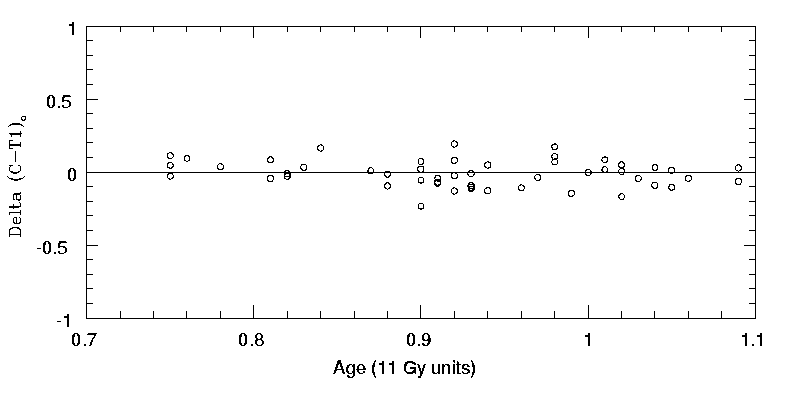
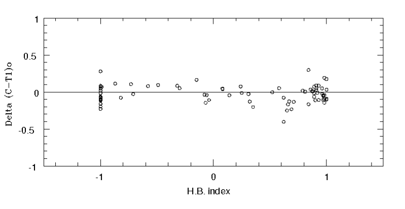
Figure 8: Upper panel: $(C-T_{1})_{o}$ colour residuals from the mean colour-metallicity calibration for MW clusters included in Figure 7 as a function of normalised ages available in de Angeli et al. (2005). Lower panel: (C-T₁)o colour residuals for MW clusters included in Figure 7 and horizontal branch morphologies (HB index) available in Mackey & van den Bergh (2005). No significant trends are detectable

We note that the shape of the empirical calibration is similar, to within $\pm$ 0.015 mags. in (C-T₁), with the colours of the 12 Gy model, with a Salpeter luminosity function and blue horizontal branch, given in Maraston (2004). This agreement is reached after subtracting a zero point difference of 0.065 mags. to their (B-I) model colours and then transforming to (C-T₁) through the relation given above. Note that these models (shown as triangles in Figure 7) are given as a function of total abundance [Z/H].

Figure 7 also includes, as a reference, the NGC 1399 nucleus according to the photometry by Ostrov et al. (1993) and the metallicity ($[Fe/H]=0.4$) obtained by Pickles (1985).

6 The globular clusters projected areal density distributions

As shown in FFG05 (figure 5) the slope of the areal density of the bluest GCs (i.e., bluer than the blue peak at (C-T₁)=1.26) in NGC 1399 is significantly shallower than that corresponding to the “whole” blue population (i.e., all clusters bluer than the colour valley at (C-T₁)=1.55) in the inner region of the galaxy. At larger galactocentric radii, these slopes become identical within the uncertainties. The significance of that result is analysed in this section on the basis of the new data set presented in this work.

First, we focus on the areal density distributions of clusters in the inner regions of both galaxies. The size of this region was defined aiming at: a) including a large number of cluster candidates; b) keeping the overall completeness level of the sample at $\approx$ 95% ; c) minimising the fraction of contaminating non-resolved field interlopers (19% and 11% for NGC 1399 and NGC 4486, respectively).

These requirements are met within a circular annulus with inner and outer radii of 120 and 420 arcsec. Within 120 arcsec the searching routines are affected by the galaxy halo brightness while, further out in galactocentric radius, the background level increases and the effective areal coverage of our images decreases.

We also set a magnitude range (T₁=21.0 to 23.2) for two reasons. On one side, in order to avoid the eventual presence of very bright objects whose nature might be connected with Omega Cen-like objects or compact dwarf galaxies (e.g. see Phillips et al. 2001). On the other, the GCs colour distribution becomes ”unimodal” in NGC 1399 (Ostrov et al. 1998) making difficult a separation between blue and red GCs.

Given the relatively small angular scale of this analysis we adopt $r^{1/4}$ laws in order to obtain least squares fits to the logarithmic surface densities within concentric circular annuli (one arcmin wide):

$$log(den)=ar^{1/4}+b$$ (15)

The resulting slopes and their associated uncertainties are listed in Table 3 and depicted in Figures 9. The upper two fits, in each panel, belong to the red and blue globulars defined in terms of the colour valleys at (C-T₁)=1.55 and 1.52 for NGC 1399 and NGC 4486, respectively. These fits, that correspond to the regions with the highest GCs areal densities, are later overlapped (Figures 11, 12 , 17 and 18) with profiles that extend to larger galactocentric radii.

Table 3: $r^{1/4}$ law fits to logarithmic areal densities for globular clusters (T₁=21.0 to 23.0)

colour range	a (slope)	b (zero point)	rms
NGC 1399
1.55 - 2.30	-0.77 $\pm$ 0.03	3.64 $\pm$ 0.11	0.02
0.90 - 1.55	-0.43 $\pm$ 0.10	2.28 $\pm$ 0.41	0.08
0.90 - 1.26	-0.25 $\pm$ 0.11	1.20 $\pm$ 0.43	0.08
NGC 4486
1.52 - 2.30	-0.91 $\pm$ 0.08	4.26 $\pm$ 0.34	0.06
0.90 - 1.52	-0.46 $\pm$ 0.04	2.87 $\pm$ 0.20	0.04
0.90 - 1.21	-0.22 $\pm$ 0.03	1.64 $\pm$ 0.12	0.02

Figure 9: Upper panel: Projected areal density for clusters in NGC 1399. The upper line belongs to clusters redder than (C-T₁)=1.55 (“red” globulars). The intermediate line corresponds to clusters with colours between 0.9 and 1.55 (“blue” globulars according to the most usually adopted definition). The lowest line belongs to clusters bluer than the blue peak at (C-T₁)=1.26 (or “genuine” blue clusters according to the text). Lower panel: Projected areal density for clusters in NGC 4486. The upper line belongs to clusters redder than (C-T₁)=1.52 (“red” globulars). The intermediate line corresponds to clusters with colours between 0.9 and 1.52 (“blue” globulars according to the most usually adopted definition). The lowest line belongs to clusters bluer than the blue peak at (C-T₁)=1.21 (or “genuine” blue clusters according to the text).

In turn, the lower fits belong to GCs bluer than the respective blue peaks (at C-T₁=1.26 and 1.21). Both galaxies show very similar behaviours in in the sense that the bluest globulars exhibit significantly shallower density slopes as found in FFG05 for the case of NGC 1399 but using Washington photometry from Dirsch et al. (2003).

A further analysis, adopting different colour windows, shows no meaningful differences in the slopes of the clusters redder than the colour valley, and we consider that they “genuinely” belong to a single population.

The intermediate slope value observed for the whole blue GCs sample (compared to the bluest GCs) tentatively suggests that an overlap between the blue and red globular subpopulations may occur in the colour range defined between the blue peak and the colour valley. This overlap would increase the density slope of the so far called blue clusters as result of the presence of the blue tail of the red subpopulation within their formal domain (i.e., objects bluer than the colour valley).

That effect should decrease with increasing galactocentric radius, as the presence of the red clusters becomes less prominent due to the steeper density profile of these clusters. This tentative picture is discussed in the following sections.

7 The case of NGC 1399

1) Colour histogram decomposition.

The background corrected GCs colour histogram is compared in Figure 10 with a synthetic one derived through the modelling described in Section 4. This histogram includes $\approx 1000$ GCs candidates with T₁=21.0 to 23.2 and (C-T₁)=0.90 to 2.30.

The decomposition process yields 620 clusters to the red subpopulation with an abundance scale factor $Zs(red)=1.45\pm 0.1Z_{\odot}$. The remaining 380 globulars are identified as belonging to the blue population with an abundance scale $Zs(blue)=0.045\pm 0.01Z_{\odot}$. Figure 10 (lower panel), with comparison purposes, also displays the Gaussian components that give the best fit to the observed histograms (blue clusters: $\overline{(C-T_{1})}=1.26$, $\sigma_{b}=0.12$; red clusters: $\overline{(C-T_{1})}=1.77$, $\sigma_{r}=0.20$). These fits decrease the number of red clusters and increase the number of blue ones suggesting a smaller degree of colour overlapping between both GCs subpopulations in comparison with the results from the model.

As discussed below, the eventual inclusion of a blue tilt comparable with that adopted for the NGC 4486 blue GCs does not have a detectable effect on the shape of the colour histogram.

Figure 10 suggests that a single abundance scale parameter for the red GCs population falls somewhat short in the extreme red end of the colour histogram. About 5% of that population appears definitely redder than the model prediction. A tentative explanation might suggest some degree of field contamination in that colour range or a possible effect connected with a variation of the $[\alpha/Fe]$ ratio with age (Kravtsov, 2007).

Figure 10 also shows that the model colour distribution of the red GCs exhibit a “blue” tail (i.e., clusters bluer than the colour valley at (C-T₁)=1.55), representing about 31% of the total number of red clusters.

These objects appear as “contaminating” the formal domain of the genuine blue globulars and will have an impact on the density slopes derived for this last population if only the colour valley is adopted as a discriminating criteria between both GCs subpopulations.

Figure 10: Globular populations fit to the background corrected colour histogram for clusters in NGC 1399 is depicted in the upper panel. The vertical line at (C-T₁)=1.55 is the colour “valley” usually adopted as the boundary between both subpopulations. The lower panel shows each of the globular populations derived from exponential distributions in the abundance domain Z. Vertical lines indicate the colours peaks of each clusters populations. Dotted lines in the lower panel show the components of the best Gaussian fit.

Alternatively, the model blue GCs barely reach the colour valley, suggesting that this population will not affect the estimate of the areal density slope of the red clusters if only clusters redder than the colour valley are included in the sampling.

2) The areal density distribution of the blue and red globulars.

Due to the features discussed in the previous item, we only take clusters bluer than (C-T₁)=1.25 (the blue peak) as tracers of the surface density of the genuine blue GCs. Figure 10 shows that there would still be a small degree of contamination by the bluest clusters of the red population (about 5% of the total sample within that colour range).

The density run with galactocentric radius of these clusters is depicted in Figure 11. In this case we only include objects with T₁=21.0 to 23.2 taken from the photometric work by Bassino et al. (2006), that reaches a galactocentric radius of 40 arcmin. The short straight line represents the density fit discussed in Section 6 while the continuous line comes from projecting on the sky a volumetric density profile:

$$\rho(a)=C(1.0+(a/rs))^{-3}$$ (16)

where $a$ is measured along the galaxy major axis, a scale length $rs=375$ arcsec and a spatial cut-off at a galactocentric radius of 450 kpc.

Figure 11: Large scale areal density distribution for globular cluster bluer than the blue peak at (C-T₁)=1.26. This colour domain is practically uncontaminated by the blue tail of the red globulars population and considered as the real distribution of the “genuine” blue globulars. The filled black dots come from data in Bassino et al. (2006). The continuous line is projected areal density described in text. The short straight line is the fit for the bluest globulars in our photometry as depicted in Figure 9

.

The large scale density distribution for the red GCs was then derived using only clusters redder than (C-T₁)=1.55 as tracers of that population and is shown in Figure 12. The short straight line is the fit discussed in Section 6 while the continuous line is a Hubble profile with a core radius r_c=60 arcsec.

Figure 12: The same as figure 8 but for clusters redder than (C-T₁)=1.55. The continuous line is a Hubble profile with a core radius r_c=60 arcsec. The short straight line is the fit for the red globulars in our photometry as depicted in Figure 9.

In order to estimate the density distribution of the total number of clusters for each population, the density of the tracer GCs should be increased by factors that take into a account the total colour range covered by these populations (adding the blue clusters redder than the blue peak and the red clusters bluer than the colour valley, respectively), as indicated by the colour histogram modelling, and also the sampled fraction of globulars within their respective integrated luminosity functions.

Grillmair et al. (1999) have derived the luminosity functions of both blue and red GCs populations in NGC 1399 on the basis of HST WFPC2 observations. Assuming fully Gaussian luminosity functions, and transforming (B-I) colours to (C-T₁), their results lead to turn overs at T₁=23.40 and T₁=23.45 with dispersions of 1.24 and 1.16 mags for the blue and red populations respectively.

The combined colour and luminosity completeness factors are then, 4.28 for the blue globulars and 3.29 for the red GCs.

3) The surface brightness profile.

Surface brightness photometry for NGC 1399 in the B band up to a galactocentric radius of 775 arsecs was presented in FFG05 and compared with other profiles available in the literature (e.g. Schombert 1986; Caon et al. 1999).

The predicted blue profile was obtained through the procedure described in Section 4 and adopting a distance modulus (V-Mv)_o=31.4, corresponding to 19 Mpc (see FFG05 and references therein), and an interstellar colour excess E(B-R)=0.011 (transformed from Schlegel et al. 1998).

Azimuthal counts do not show a detectable flattening of the NGC 1399 GCS and therefore we adopted the average flattening of the galaxy, q=0.86, as representative for both cluster populations.

The model surface brightness profile delivered by ELLIPSE is compared with the FFG05 observations in Figure 13 and corresponds to $\gamma=0.82(\pm 0.05)\times 10^{-8}$ and $\delta$=1.1 $\pm$ 0.1. The overall rms of the fit is $\pm$ 0.035 mags.

Figure 13: Observed B surface brightness profile for NGC 1399 (FFG05; filled dots) confronted with the model fit (open circles). This last profile was obtained from a bi-dimensional model image processed with the ELLIPSE task within IRAF. Squares and triangles represent the luminosity associated with the “blue” and “red” stellar populations. Note that the model fails inside 100 arcsec in galactocentric radius where the globular distributions shows a flat core.

8 The case of NGC 4486

1) Colour histogram decomposition.

Figure 14: A globular population fit to the background corrected colour histogram for clusters in NGC 4486 (see Figure 4) is depicted in the upper panel. The vertical line at (C-T₁)=1.52 is the colour “valley” usually adopted as the boundary between both populations. The lower panel shows each of the globular populations derived from exponential distributions in the abundance domain Z. Vertical lines indicate the colour peaks of each cluster populations. Dotted lines in the lower panel show the components of the best gaussian fit.

The GCs background corrected colour histogram is compared with the model fit in Figure 14. In this case, 800 clusters were assigned to the red population with an abundance scale $Zs(red)=0.90\pm 0.1Z_{\odot}$ and 1000 clusters to the blue population with $Zs(blue)=0.012\pm 0.005$ practically unde Z_⊙ (see below). Figure 14 also shows the Gaussian components (blue clusters: $\overline{(C-T_{1})}=1.21$, $\sigma=1.12$; red clusters: $\overline{(C-T_{1})}=1.72$, $\sigma=0.20$). Here we also adopt an initial abundance $Zi=0.003Z_{\odot}$ for the red clusters. However, as shown in Section 3, the blue GCs display an evident tilt that we associate with a change in abundance that correlates with the cluster brightness and, hence, mass (see also figure 3 in Brodie & Strader 2006). In this case, we find that a change in initial abundance as a function of brightness:

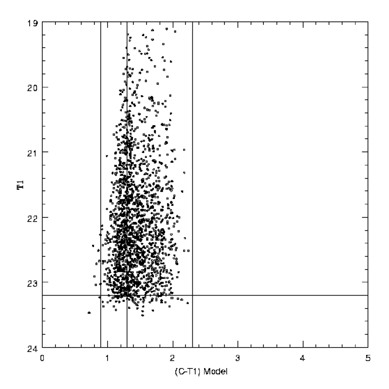
Figure 15: Model colour diagrams with $Zs(blue)=0.012Z_{\odot}$ (left panel) and $Zs(blue)=0.05Z_{\odot}$. Both models include a blue tilt similar to that discussed in the text. However, the larger Zs(blue) adopted in the right panel, makes more difficult the detection of the tilt.

$$\Delta Z=0.01(23.2-T_{1})~{}~{}~{}~{}(Z_{\odot}~{}~{}units)$$ (17)

reproduces the appearance of the blue GCs colour-magnitude diagram. The mean Z for blue GCs with T₁ from 21.0 to 21.25 mags. is $0.0371Z_{\odot}$ while for clusters with T₁ from 22.95 to 23.2 is $0.017Z_{\odot}$. These values are consistent with a mass/metallicity scaling relation (where M is the clusters mass):

$$Z\approx M^{0.44}$$ (18)

somewhat smaller than $Z\approx M^{0.55}$ but comparable to $Z\approx M^{0.48}$ suggested respectively by Harris et al. (2006) and Strader et al. (2006). Figure 3 also suggests that the blue GCs tilt, as noted by the last authors, is in fact detectable over the whole magnitude range brighter than T₁=23.2.

As mentioned in Section 3, a tilt is not detected in the case of the NGC 1399 GCs. In this galaxy, blue GCs exhibit a considerably larger Zs(blue) than in NGC 4486 and we suggest that, this larger abundance spread makes more difficult the detection of an eventual tilt. As an example, Figure 15 displays the colour magnitude diagram for the adopted model in the case of NGC 4486, showing the blue tilt (left panel). An increase of Zs(blue) from 0.012 to 0.05 (comparable to that of the blue GCs in NGC 1399) changes substantially the appearance of that diagram and makes the blue tilt (included in the model) less evident (right panel).

2) The areal density distribution for blue and red clusters.

Figure 16: Azimuthal counts (within 22.5 degrees bins) for the globular clusters brighter than T₁=23.2 and (C-T₁) from 0.9 to 2.3 (large filled dots). The statistical uncertainty of the counts is shown with bars. Open dots come from a composite model that includes red clusters with a flattening q=0.8 and blue clusters with q=0.5 according to text.

The fact that the NGC 4486 GCS exhibits a noticeable flattening has been pointed out by McLaughlin et al. (1994). This feature is clearly seen in Figure 16, which shows azimuthal counts within a galactocentric circular annulus with inner and outer radii of 120 and 360 arcsec, performed using our photometry (T₁=21 to 23.2 and (C-T₁)=0.90 to 2.30). This figure also displays the results from a model that includes red GCs with a flattened spatial distribution with q=0.80, and blue clusters with q=0.50 (where q=b/a, is the ratio of the minor to major semi axis). The details of this model, that provides a consistent fit to the observations, are discussed below.

The adopted flattenings come from the assumption that, if GCs trace a given stellar population, they should share the same flattening. The inner regions of NGC 4486 (where the red stellar component dominates the surface brightness) exhibits a q=0.85 (at a=120 arcsec) and reaches about q=0.50 at the outermost detectable boundaries (see Mihos et al. 2005), where the blue stellar population should become more evident.

The density run on a large angular scale was determined by using Suprime camera observations by Tamura et al. (2006b). These authors determine areal density in circular annuli on a rectangular strip that extends to the east of the galaxy centre.

We stress that, as those authors use the colour valley at (V-I)=1.10 in their photometry as a discriminant between both cluster populations, their so called blue clusters will eventually include the blue tail of the red population inferred from the colour histogram decomposition. We note that Tamura et al. also find that a projected NFW profile gives good representation of the areal density distribution of the so defined blue GCs as FFG05 did in NGC 1399 using the same definition for the blue clusters.

In order to test the compatibility of their observations with our approach, we generated a model that assumes that both cluster populations follow elliptical distributions with the flattenings mentioned before and a major axis coincident with that of the galaxy halo (P.A. $\approx$ 155 degrees).

The density distribution of the genuine blue clusters in the inner regions of the galaxy was fit using a surface density profile similar to that adopted for NGC 1399 but with a scale length rs=350 arcsec. This fit gives an adequate representation to the density depicted in Figure 9 (lower panel).

In turn, model red clusters were generated adopting a lowered Hubble density profile (or analytical King profile) with rc=60 arcsec (from Kundu & Whitmore 1998). In this case, the tidal radius was changed iteratively until the best fit to the Tamura et al. densities was obtained, yielding r_t=3600 arcsec.

Model GCs colours were generated as described above while the T₁ magnitudes were derived by adopting fully Gaussian integrated luminosity functions with turn-overs at T₁=22.9 and 23.2 and dispersions of 1.38 and 1.55 mags. for the blue and red globulars, respectively. These parameters were taken from Tamura et al. (2006a), who give values in the V band, and transformed to the T₁ band (through $(V-R)=(V-T_{1})=0.21(C-T_{1})+0.19$).

The completeness factors, that allow an estimate of the total number of GCs in each subpopulation from the fractional sampling in colour and magnitude, were 3.20 for the blue GCs and 3.31 for the red GCs.

The combined cluster population was then sampled in circular annuli, in order to compare with the Tamura et al. density profile and taking those GCs bluer than the colour valley at (C-T₁)=1.52 (or (V-I) $\approx$ 1.10, following their definition of the blue population).

The result for this blue population (shifted in log (dens.)) is shown in Figure 17 that also includes a straight line that represents the NFW profile (rs=226 arcsec; 20 kpc at their adopted galaxy distance) fit by Tamura et al. (2006a) to this cluster population. The lower line in this diagram corresponds to the genuine blue GCs and comes from sampling, also in circular annuli, the projection on the sky of an oblate ellipsoid (with q=0.5). This ellipsoid follows the blue GCs spatial density dependence mentioned above with a cut off at 450 kpc from the galaxy centre.

Figure 17: Projected areal distribution for NGC 4486 GCs bluer than the colour valley. Filled dots come from counts within circular annuli given by Tamura et al. (2006b). Open dots are from the model described in the text. The straight line is the NFW fit given by those authors. Note that, following this colour definition, the so called “blue” globulars do not exhibit the flat inner core. The adopted distribution of the “genuine” blue globulars is also shown (lower curve). The dashed line has the slope shown in figure 9 for GCs bluer than (C-T₁)=1.21.

Figure 17 in fact shows that the model discussed in this section is able to match the Tamura et al. density profile, which does not show a flat core.

The difference between this last profile and the adopted one for the genuine blue GCs, can thus be explained as the result of including the blue tail of the red cluster population, characterised by a steeper spatial distribution, within the sample of GCs bluer than (V-I)=1.10.

Figure 18, in turn, shows the comparison of the model with the red GCs as defined by Tamura et al. which, not suffering the colour overlapping effect, is directly comparable with our model red clusters.

Figure 18: Projected areal distribution for NGC 4486 GCs redder than the colour valley (“red” globulars). Filled dots come from counts within circular annuli given by Tamura et al. (2006b). Open dots come from the model described in the text. The model counts have been shifted vertically in order to take into account the limiting magnitude in that work. The dashed line has the slope shown in Figure 9 for GCs redder than C-T₁=1.72.

3) The surface brightness profile.

Two blue surface brightness profiles with a relatively large angular coverage are available for NGC 4486 in the literature: Carter & Dixon (1978) and Caon et al. (1999). These profiles, along the major axis of the galaxy, show good agreement up to a $\approx$ 600 arcsec where the Caon et al. profile becomes systematically fainter. A comparison with the diffuse light map in the Virgo cluster by Mihos et al. (2005), in turn, indicates a V surface brightness V $\approx$ 26.5 mags. per arcsec${}^{\sq}$ at a $\approx$ 1800 arcsec that imply B= 27.1 to 27.5 mags. per arcsec${}^{\sq}$ which is consistent with the Carter & Dixon profile which we adopt in what follows.

Figure 19 shows the best fit profile obtained through ELLIPSE from the blue synthetic image. The profile corresponds to a distance modulus (V-Mv)_o=31.0 and an interstellar reddening E(B-V)=0.022 from Schlegel et al. (1998).

Figure 19: Observed B surface brightness profile for NGC 4486 ( Carter & Dixon 1978; filled dots) confronted with the model fit (open circles). This last profile was obtained from a bi-dimensional model image processed with the ELLIPSE task within IRAF. Squares and triangles represent the luminosity associated with the “blue” and “red” stellar populations. Note that the model fails inside 100 arcsec in galactocentric radius where the globular distributions shows a flat core.

The profile fit requires $\gamma=1.18(\pm 0.05)\times 10^{-8}$ and $\delta=1.2\pm 0.1$ with and yields an rms of $\pm$ 0.07 mags. Again, and as already noted for NGC 1399, the flat core of the GCS does not allow a proper representation of the inner region of the galaxy.

The ouput from ELLIPSE shows that, as a result of composing two diffuse populations with different flattenings, the galaxy model flattening varies with galactocentric radius. This trend is compared with the ellipticity values ($\epsilon$=1-q) obtained by Carter & Dixon (1978) in Figure 20. The overall agreement is acceptable although it could be improved if the possibility of a variable q (for one or both cluster subpopulations) is allowed. However, the statistical uncertainties connected with the azimuthal counts prevents a meaningful estimate of this eventual dependence.

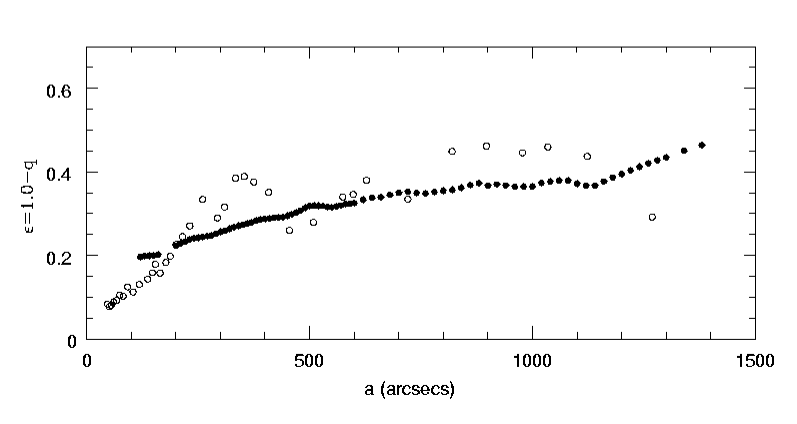
Figure 20: Ellipticity ($\epsilon=1-q$) variation of the NGC 4486 stellar halo as a function of semi-major axis $a$ from Carter & Dixon (1978) (open circles), compared with the expected variation from the model fit (filled circles).

9 Dependence of Results on Uncertainties of the Fitting Parameters

The overall results from this modelling in terms of specific frequencies, characteristic t* parameter (integrated over metallicity for each of the cluster populations), diffuse stellar mass and $(M/L)_{B}$ ratios are listed in Table 4 .

Table 4: Model results for NGC 1399 and NGC 4486.

	NGC 1399	NGC 4486
Adopted (V-Mv)o	31.4	31.0
Zs(blue)	0.045	0.012	a
Zs(red)	1.45	0.90
$\gamma$	0.82$\times 10^{-8}$	1.18$\times 10^{-8}$
$\delta$	1.10	1.20
number of blue globs.	3900	7000	b
number of red globs.	4500	4800	b
$Sn^{*}$(blue globs)	12.1	27.9	c
$Sn^{*}$(red globs)	5.3	8.4	c
t* (blue globs)	3.44$\times 10^{-8}$	8.41$\times 10^{-8}$	d
t* (red globs)	0.85$\times 10^{-8}$	1.43$\times 10^{-8}$	d
t* (total)	1.3$\times 10^{-8}$	2.82$\times 10^{-8}$	d
$(M/L)_{B}$ (blue pop)	4.2	3.9
$(M/L)_{B}$ (red pop)	9.6	8.7
Total stellar mass ($M_{\odot}$)	7.2$\times 10^{11}$	4.8$\times 10^{11}$	e
Frac. mass (blue pop.)	0.18	0.20
Frac. mass (red pop.)	0.82	0.80
a) Plus a blue “tilt”: $\Delta Z=0.01(23.2-T_{1})$
b) Inside a=1500 arcsec, assuming Gaussian LFs
c) Intrinsic values defined in terms of their associated stellar
luminosities in the V band.
d) Integrated values defined in terms of their associated stellar masses.
e) Inside a projected galactocentric radius of 100 kpc

The total stellar masses given in this table include a correction that takes into account the region within 120 arcsec in galactocentric radius, where the model does not provide an adequate fit.

In what follows we describe the uncertainties of these results in terms of the fitting parameters, $\gamma$ and $\delta$, as well as those connected with the colour-metallicity relation, (M/L) ratios, age, and adopted abundance scale.

-$\gamma$ parameter:

Figure 21 depicts the dependence of both $\gamma$ and total projected stellar mass (within a constant galactocentric radius of 100 kpc) with distance modulus. The adopted distance moduli for both galaxies are also shown along with a (formal) associated uncertainty of $\pm 0.25$ mags. Even such small uncertainties, do not rule out that both galaxies might be at similar distances from the Sun, and in this case, the $\gamma$ parameter and total stellar masses of NGC 1399 and NGC 4486 would also be very similar.

-$\delta$ parameter:

$\delta$ is independent of the adopted distance and a variation of the order of the fit uncertainty ($\pm 0.1$), mainly impacts on the total mass of the diffuse stellar population associated with the blue GCs, that changes by $\pm 15\%$.

Larger $\delta$ values imply a decrease in the mass of these stars and also redder integrated colours of the composite stellar population.

Figure 21: Variation of the $\gamma$ parameter (lower curves) and total projected stellar mass within 100 kpc (upper curves) obtained from model fits as a function of the adopted distance modulus (solid line: N1399; dashed: NGC 4486). Horizontal lines indicate a change of $\pm 0.25$ mags. around the adopted distance moduli.

-M/L ratio and age:

The (M/L) ratio depends on the age and metallicity of the seed GCs. We tentatively adopt an age of 12 Gy comparable to that of the Milky Way System (see, for example, de Angeli et al. 2005).

Synthetic population models by Worthey (1994) show that a variation of $\pm 2$ Gy around the adopted model age increases or decreases those ratios by 15% without changing the shape of the functional dependence with metallicity. Accordingly, masses also change in the same proportion. Age variations of that order however, do not have a noticeable impact on either the shape of the brightness profile or its integrated colour.

The characteristic $(M/L)_{B}$ ratios for both diffuse populations (as well as for the composite stellar population) were obtained by integrating over the whole range of abundances determined by their respective abundance scale lengths and adopting an upper cut off of $4Z_{\odot}$. These results are not critically dependent upon this formal upper limit.

In particular, we note that the $(M/L)_{B}$ values of the red stellar populations are comparable to that obtained by Saglia et al. (2000) ($(M/L)_{B}=10$ ) in the case of the central regions of NGC 1399 where the red population dominates the integrated luminosity.

-Abundance scale:

The relation between [Fe/H]zw and [Z/H], adopted as a constant over the whole abundance range, might not be totally appropriate since the Mendel et al. (2007) work does not include GCs at a very low abundance regime. We also attempted models adopting the Mendel et al. [Z/H]-[Fe/H]zw off set value (0.131) for the red GCs and a tentatively larger value (0.3) for the blue clusters. This modification leads to larger $(M/L)_{B}$ ratios for the blue population and to an increase of the total mass of about 20% (although no significant improvement of the fits of the colour histograms is obtained).

10 Implications of the profile fit

The $\gamma$ and $\delta$ parameters that provide the best fit to the shape of the B band surface brightness profile of each galaxy will also lead to a given:

1. Galactocentric colour gradient of the galaxy halo.

2. Colour off-set between GCs and galaxy halo.

3. Behaviour of the cumulative GCs specific frequency with galactocentric radius.

4. Metallicity distribution of the diffuse stellar population.

A comparison of these predicted features with the observed ones, as follows, then may provide independent clues about the success of the model.

a) Galactocentric colour gradient of the galaxy halo.

The main implication of the model is that, at galactocentric distances larger than 120 arcsec, the main driver of the galaxy colour gradient is the (luminosity weighted) composition of the associated blue and red diffuse stellar populations.

FFG05 presented the expected colour (B-R) gradient for the NGC 1399 halo on the basis that the colours of the diffuse stellar populations could be identified with the colours of the peaks of the associated GCs. That assumption is no longer necessary in this work as the colour of each mass element connected with a given globular, as well as its mass to luminosity ratio, are determined by the metallicity of the “seed” cluster.

b) Globulars-galaxy halo colour off set.

The GCs mean integrated colours (including all clusters) in massive elliptical galaxies usually exhibit a galactocentric colour gradient comparable to that of the galaxy halo but blue ward shifted (Strom et al. 1981; Forte et al. 1981).

In the context of the model discussed in this work, the cluster gradients arise as a consequence of (number weighting) averaging the two GCs subpopulations, characterised by different spatial scale lengths. The same reasoning apply to the associated diffuse stellar populations but, in this case, weighted through the (M/L) ratios determined by metallicity, then leading to the observed colour off-set.

Colour gradients derived from the profile fits are shown in Figure 22. In these diagrams, the predicted halo colours are compared with the mean globular integrated model colours and also with those obtained from the photometry presented in section II. These diagrams show that, in fact, the galaxy halos exhibit colour gradients comparable, but redder, than those of the GCs.

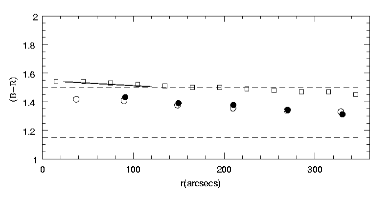
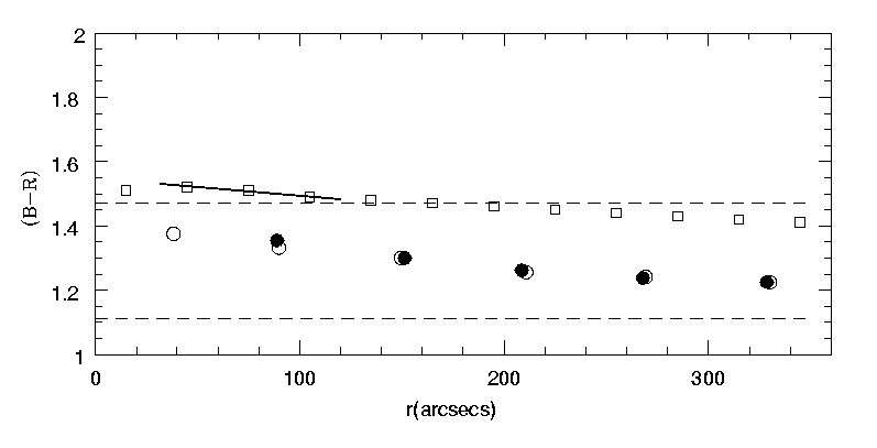
Figure 22: (B-R) colour gradient as a function of galactocentric distance for the halo (open squares) compared with the mean globular cluster colours from the model fit (open circles). The globular mean observed colours, derived from the photometry presented in this paper, are also shown (filled circles). The short straight line indicates (B-R) colours derived from Michard (2000). Upper panel: NGC 1399; Lower panel: NGC 4486. The dashed lines indicate, for each galaxy, the peak colours of the blue and red GCs.

Figure 22 also shows that the (B-R) colour gradients determined by Michard (2000) in the inner regions of the galaxies are in very good agreement with with the predicted colours of the halo.

c) Cumulative globular cluster specific frequency.

Figure 23 shows the galactocentric variation of the cumulative specific frequency derived from the best fit models. The GCs populations inside a galactocentric radius of 120 arcsec were taken from Forbes et al. (1998) and Kundu & Whitmore (1998). Even though each cluster subpopulation has its own intrinsic frequency, a variation of the composite Sn is expected as the number ratio of blue to red GCs changes with galactocentric radius.

The parametric Sn values (McLaughlin et al., 1994), defined at a galactocentric radius of 40 kpc, from this figure are $Sn\approx 3.5$ and $Sn\approx 8.5$ for NGC 1399 and NGC 4486, respectively. These values are considerably lower than previous estimates given in the literature as already noted in Forte et al. (2002).

Figure 23: Cumulative globular cluster specific frequencies for NGC 1399 (lower curve) and NGC 4486 (upper curve) derived from the model fits. The vertical lines indicate galactocentric radius of 40 kpc (dotted line: NGC 1399; dashed line: NGC 4486) and indicate $Sn\approx 3.5$ and $Sn\approx 8.5$, respectively.

d) The metallicity distribution of the diffuse stellar population.

The shape of the [Fe/H] distribution expected for the diffuse stellar population was schematically derived in FFG05 on the basis of estimating a characteristic $(M/L)_{B}$ ratio and intrinsic specific frequency for each cluster population. In contrast, in this work each stellar mass element has a given metallicity, and hence (M/L) ratio. The statistic distribution of these masses, as a function of [Fe/H] is given in Figure 24 for NGC 1399 and NGC 4486. For both galaxies we show the inferred metallicity distribution, for galactocentric ranges from 10 to 15 and 15 to 25 kpc convolved with a Gaussian kernel (dispersion: 0.20 dex) aimed introducing some degree of smoothing comparable to observational errors.

Figure 24: Stellar mass histogram as a function of metallicity for NGC 1399 (upper panel) and NGC 4486 (lower panel). These histograms belong to elliptical galactocentric radii between 10 and 15 kpc (solid line) and 15 to 25 kpc (dotted line) at an adopted distance of 19 Mpc (NGC 1399) and 15.8 Mpc (NGC 4486). The histograms asume an $\alpha$ ratio of 0.3

These mass statistics can be transformed into star-number ones under the assumption that the stellar luminosity functions do not depend strongly on metallicity. A comparison with the cases of NGC 5128 (Harris & Harris 2002 or Rejkuba et al. 2005) and also M31 (Durrell et al., 2001) shows good qualitative agreement, i.e, the presence of a broad high metallicity component and an extended tail towards low metallicity that becomes more evident as galactocentric radius increases. More recently, Mouhcine (2006) presents stellar number statistics for a number of edge on spirals which also shows low metallicity skewed distributions, a feature that seems independent of the galaxy morphology.

11 Caveats about the model

The model described in this work has several caveats, namely:

-colour bimodality is attributed to two different GCs subpopulations. An alternative view, based on the presence of an inflection region in the colour-metallicity relation as the main driver of the shape of the colour histograms, has been suggested by Yoon et al. (2006). So far, however, neither our calibration nor recent spectroscopic results in NGC 4472 (Strader et al., 2007) seem to support that situation. Further results in this last direction can also be found in Kundu & Zepf (2007) for the case of NGC 4486.

- Although an exponential dependence of the number of GCs with abundance was adopted, more complex functional dependences, hidden by the noise of the GCs statistics, could not be ruled out.

- An abundance dependence with brightness, that leads to a blue tilt in the case of the blue GCs, is included in the models. However, we cannot infer whether the tilt is just a local effect or if it is actually shared by the diffuse stellar population associated with the blue clusters. Nevertheless removing the tilt from the models, has little impact on the output integrated colours that then would become slightly bluer ($\approx 0.015$ mags. in (B-R)).

-The two dominant cluster subpopulations are assumed to be coeval. Further refinement of this aspect could be incorporated once meaningful ages become available. On one side some works (e.g Jordan et al. 2002) do not find detectable age differences between the blue and red populations in NGC 4486. On the other, (e.g. Forbes et al. 2001; Pierce et al. 2006a; Pierce et al. 2006b, or Hempel et al. 2007) do find a certain fraction of intermediate age clusters in NGC 1399 and in other galaxies.

-The $[\alpha/Fe]$ is adopted as constant and equal for the cluster subpopulations in both galaxies in order to derive the [Fe/H] stellar distributions . Even though the adopted value is appropriate for the MW (see Carney 1996, or Thomas et al. 2003) and also representative for ellipticals (Puzia et al., 2005), a possible variation with metallicity as noted by these last authors and, earlier, by Shetrone, Côté & Sargent (Shetrone et al.2001), cannot be ruled out.

12 Discusssion and Conclusions

The results presented in previous sections show that the surface brightness profiles of both NGC 1399 and NGC 4486 can be traced using a common link between GCs and the stellar halo populations in these galaxies. This link imply that the number of GCs per diffuse stellar mass, defined as $t=\gamma\exp(-\delta[Z/H])$ ,increases when chemical abundance decreases. We note that Harris & Harris (2002) had already found an increase of Sn with decreasing GCs metallicity in the case of NGC 5128.

This suggests that, on a large scale, the dominant globular cluster subpopulations formed along major star forming episodes and following a similar pattern. However, it is not yet clear whether abundance, through the role that it plays in the t parameter, is the physical reason that governs the fraction of clustered to diffuse stellar mass or, eventually, some other “hidden” variable in turn correlated with abundance.

The quality of the profile fits is comparable to any other parametric approximation in a range that covers a galactocentric radius from 10 to 100 kpc. In the inner regions, GCs fail to map the brightness distribution probably as a consequence of cluster destruction processes due to gravitational effects. However, it seems that survivor clusters, with large perigalacticon orbits, are still able to trace their associated stellar populations. It is worth mentioning that, based on far UV observations of NGC 1399 , Lotz et al. (2000), find arguments that support the coexistence of two widely different stellar populations, in terms of chemical abundance, in the nucleus of the galaxy.

Even though the approach only aims at reproducing the brightness profiles, other connected features as galactocentric colour gradients, GCs-halo colour offset, cumulative cluster specific frequency and inferred stellar metallicity distributions compare very well with observations.

It seems also remarkable that the common quantitative GCs-stellar halo link works in both galaxies although their cluster populations exhibit detectable differences in cluster numbers and chemical abundance. Both GCs subpopulations have larger abundance scale lengths (as defined in Section 4) in NGC 1399 than in NGC 4486 leading to total mean abundance ratios of 1.4 and 2.5 for the red and blue GCs, respectively.

As shown in Figures 10 and 14, the approach presented in this paper delivers GCs colour distributions that are not strongly different from a two Gaussians fit requiring five free parameters, a common procedure in the literature (e.g Ostrov, Forte & Geisler 1998). However, we note that our models indicate a lower ratio of the number of blue to red GCs and only require three free parameters.

Blue GCs in NGC 4486 have a small abundance scale lenght, about four times smaller than that of the blue GCs in NGC 1399, and we speculate that this may be connected with a shorter formation time scale. In turn, that lower abundance spread may be the reason behind the presence of a blue tilt, connected with cluster mass, in the colour magnitude diagram. This feature seems absent, or probably masked, by the larger abundance scale of the blue GCs in NGC 1399, a situation that may also hold in other galaxies (e.g. NGC 4472, Strader et al. 2006).

This last result argues in favour of the idea that blue GCs “know” about the galaxy they are associated with (Strader, Brodie & Forbes 2004). In any case, and in both galaxies, the blue GCs barely reach an abundance close to [Z/H]=-0.5. The reason for this upper metallicity cut off may be connected with some kind of sincrhonising event as the re-ionisation of the Universe (Cen 2001; Santos 2003; Rhode & Zepf 2005). However, the different abundance scale lengths of the blue GCs also suggest that a local phenomenon, distinct for each galaxy, may have also played a role in modulating the the star formation rate (e.g. the onset of galaxy nuclear activity).

The overall picture seems consistent with some scenarios already discussed in the literature (Forbes et al. 1997; Harris et al. 2006) that invoke two different cluster formation mechanisms and, probably, environmental conditions.

In contrast with the relative abundance homogeneity and large spatial (half density) core radii ($\approx$ 25 kpc) of the blue GCs, the red ones exhibit a large abundance heterogeneity and much smaller core radii ($\approx$ 5 kpc) also shared by the red diffuse stellar population. This degree of heteregeneity may be connected , for example, to mergers of different nature (e.g. Schweizer & Seitzer 1993).

The total globular cluster formation efficiencies, in terms of stellar mass, indicated by the models, and adopting an average cluster mass of $2.5\times 10^{5}M_{\odot}$, are $2.4\times 10^{-3}$ for NGC 1399 and $5.6\times 10^{-3}$ for NGC 4486. They are comparable to the efficiency derived by McLaughlin (1999) although, in that case, the definition of efficiency included total baryonic mass.

Blue clusters show a higher formation efficiency (in terms of the stellar mass they are associated with), when compared with the red ones, probably as a consequence of a lower star formation efficiency during the early phases of galaxy formation at a low metallicity regime.

Although there is no strong evidence of an age difference between the blue and red globular subpopulations (e.g. Jordan et al. 2002) within the uncertainties of the measurements, a possible temporal sequence that assumes the formation of the blue population first, cannot be discarded as a result of the relatively small time scales involved at the early phases of galaxy formation (see Beasley et al. 2003). In this frame, the chemical enrichment provided by a presumably progenitor blue population might be important to boost later stellar formation efficiency through an abundance enrichment that may reach $[Z/H]\approx$-0.60 within 100 kpc of the galaxy nucleus.

Some scenarios suggest that blue GCs formation is associated with dark matter (Beasley et al. 2002; Moore et al. 2006; Prieto & Gnedin 2006), and it is tempting to look for such a connection. For example, the results listed in Table 4 show that while both galaxies have a similar total number of red GCs, NGC 4486 outnumbers NGC 1399 in a factor of about 1.8 in terms of blue GCs. Dark mass estimates within a galactocentric radius of 100 kpc are 3.4$\times 10^{12}M_{\odot}$ for NGC 1399 (extrapolating data from Richtler et al. 2004) and 7.4$\times 10^{12}M_{\odot}$ for NGC 4486 (Côté et al., 1998), leading to a ratio $\approx 2.0$ comparable to that in the number of blue GCs.

The similarity of the stellar galaxy masses, and the difference in their total masses, had already been noticed by Jones et al. (1997) on the basis of their X ray analysis.

FFG05 found that, adopting their definition of blue clusters, the density profiles of the NGC 1399 GCs could be fit with a NFW profile (Navarro et al., 1996) with a scale length of 375 arcsec, coincident with that derived for the inferred dark matter halo by Richtler et al. (2004). Tamura et al. (2006a) also perform a NFW profile fit to the blue clusters in NGC 4486. However, both approaches deserve a revision since, on the basis of the results presented in this work, the “genuine” blue GCs exhibit a rather extended inner core in their surface density profiles. As shown here, these cores have been disguised by the inclusion of the blue tail of the red subpopulation within the “blue” GCs sample. This overlapping should be even more severe when using colour indices less sensitive to metallicity than (C-T₁) and should be taken into account when doing, for example, kinematic analysis of the cluster subpopulations.

References

- Ashman & Zepf (1992) Ashman, K. M. Zepf, S.E., 1992, ApJ, 384, 50
- Bassino et al. (2006) Bassino, L.P., Faifer, Forte, J.C., Dirsch, B., Richtler, T., Geisler, D., Schuberth, Y., 2006, A&A, 451, 789
- Beasley et al. (2002) Beasley, M. A., Baugh, C.M., Forbes, D.A., Sharples, R.M., Frenk, C. S., 2002, MNRAS, 333, 383
- Beasley et al. (2003) Beasley, M. A., Kawata, D., Pearce, F., Forbes, D., Gibson, B., 2003, ApJ,596, L187
- Bica et al. (2006) Bica, E., Bonatto, C., Barbuy, B., Ortolani, S., 2006, A&A, 450, 105
- Brodie & Strader (2006) Brodie, J.P., Strader, J. 2006, AR&A 44, 193
- Carney (1996) Carney, B. W., 1996, PASP 108, 900
- Caon et al. (1994) Caon N., Capaccioli, M., Donofrio, M.,A&AS, 1994, 106, 199
- Caon et al. (1999) Caon, N., Capaccioli, M., Rampazzo, R., 1999, A&AS 86, 429.
- Capuzzo-Dolcetta & Tesseri (1999) Capuzzo-Dolcetta, R., Tesseri A., 1999, MNRAS, 308, 961
- Carter & Dixon (1978) Carter D., Dixon K.L., 1978, AJ, 83, 574
- Cen (2001) Cen, R. 2001, ApJ, 560, 592
- Côté et al. (1998) Côté, P., Marzke, R. O., West, M. J., 1998, ApJ, 501, 554
- de Angeli et al. (2005) de Angeli, F., Piotto, G., Cassisi, S., Busso, G., Recio-Blanco, A., Salaris, M., Aparicio, A., Rosenberg, A., 2005, AJ, 130, 116
- Dirsch et al. (2003) Dirsch B., Richtler T., Geisler, D., Forte J.C., Bassino, L.P., Gieren, W., 2003, AJ, 125, 1908
- Durrell et al. (2001) Durrell P., R., Harris W.E., Pritchet C.J., 2001, AJ, 121, 2557
- Eggen et al. (1962) Eggen O., Lynden Bell D., Sandage A.R., 1962, ApJ, 136, 748
- Forbes et al. (1998) Forbes, D.A., Grillmair, C.J., Williger, G.M., Elson, R.A.W., Brodie, J. P., 1998, MNRAS, 293, 325
- Forbes et al. (1997) Forbes D. A., Brodie, J.P., Grillmair, C.J., 1997, AJ, 113, 1652
- Forbes et al. (2001) Forbes D. A., Beasley, M.A., Brodie, J.P., Kissler-Patig, M., 2001, ApJ, 563, 143
- Forbes & Forte (2001) Forbes, D. A., Forte, J.C., 2001, MNRAS, 322, 257
- Forbes (2005) Forbes, D.A., 2005, ApJ, 635, L137
- Forte et al. (1981) Forte, J.C., Strom, S. E., Strom, K., 1981, ApJ, 245, L9
- Forte et al. (2001) Forte, J.C., Geisler, D., Ostrov, P.G., Piatti, A.E., Gieren, W., 2001, AJ, 121, 1992
- Forte et al. (2002) Forte, J.C., Geisler, D., Kim, E., Lee, Myung Gyoon, Ostrov, P., 2001, Proceedings IAU Symp. 207, Ed. D. Geisler, E.K. Grebel, D. Minniti, 2002, 251
- Forte et al. (2005) Forte, J.C., Faifer, F., Geisler, D., 2005, MNRAS, 357, 56
- Geisler & Forte (1990) Geisler, D., Forte, J.C., 1990, ApJ, 350, L5
- Geisler (1996) Geisler, D., 1996, AJ, 111, 480
- Grillmair et al. (1999) Grillmair, C. J., Forbes, D.A., Brodie, J.P., Elson, R.A.W., 1999, AJ, 117, 167
- Harris & Canterna (1977) Harris, H.C., Canterna, R., 1977, AJ, 82, 798
- Harris & Canterna (1979) Harris, H.C., Canterna, R., 1979, AJ, 84, 1750
- Harris & van den Bergh (1981) Harris W.E., van den Bergh, S., 1981, AJ, 86, 1627
- Harris et al. (1998) Harris, W.E., Harris G.L.H., Mclaughlin D.E., 1998, AJ 115, 1801
- Harris & Harris (2002) Harris, W.E., Harris, G.L.H., 2002, AJ 123, 3108
- Harris et al. (2006) Harris, W.E., Whitmore, B.C., Karakla, D., Okon, W., Baum, W.A., Hanes, D.A., Kavelaars, J.J., 2006, ApJ, 636, 90
- Hempel et al. (2007) Hempel, M., Kissler-Patig, M., Puzzia, T.H., Hilker, M., 2007, A&A, 463, 493
- Jones et al. (1997) Jones, C., Stern, C., Forman, W., Breen, J., David, L., Tucker, W., 1997, ApJ, 482, 143
- Jordan et al. (2002) Jordan, A., Côté, P., West, M.J., Marzke, R.O., 2002, ApJ, 576, L113
- Jordan et al. (2004) Jordan, A., Côté, P., West, M.J., Marzke, R.O., Minniti, D., 2004, AJ, 127, 24
- Kravtsov (2007) Kravtsov, V. V., 2007, astro-ph 0705.2246v1
- Kundu & Whitmore (1998) Kundu, A., Whitmore, B.C., 1998, AJ, 116, 2841
- Kundu & Zepf (2007) Kundu, A., Zepf, S.E., 2007, ApJ, 660, L109
- Larson (2006) Larson, S. S., 2006, astro-ph/0606625v1
- Lee et al. (2002) Lee, H-c., Lee, Y. W., Gibson, B. K., 2002, AJ, 124, 2664
- Lotz et al. (2000) Lotz, J.M., Ferguson, H.C., Bohlin, R.C., 2000, ApJ, 532, 830
- Mackey & van den Bergh (2005) Mackey, A.D., van den Bergh, S., 2005, MNRAS, 360, 631
- Maraston (2004) Maraston, C., 2004, MNRAS 363, 131
- McLaughlin et al. (1994) McLaughlin, D.E., Harris, W.E., Hanes, D.A., 1994, ApJ, 422, 486
- McLaughlin (1999) McLaughlin, D.E., 1999, AJ, 117, 2398
- Mendel et al. (2007) Mendel, J. T., Proctor, R. N., Forbes, D. A., 2007, MNRAS, in press.
- Michard (2000) Michard, R., 2000, A&A 360, 85
- Mihos et al. (2005) Mihos, J. C., Harding, P., Feldmeier, J., Morrison, H., 2005, ApJ, 2005, ApJ, 631, 41
- Moore et al. (2006) Moore, B., Diemand, J., Madau, P., Zemp, M., Stadel, J., 2006, MNRAS, 368, 563
- Mouhcine (2006) Mouhcine, M., 2006, ApJ, 652, 277
- Navarro et al. (1996) Navarro, J.F., Frenk, C. S., White, S.D.M., 1996, ApJ, 462, 563
- Ostrov et al. (1998) Ostrov, P., Forte, J.C., Geisler, D., 1998, AJ, 116, 2854
- Ostrov et al. (1993) Ostrov, P., Geisler, D., Forte, J. C., 1993, AJ, 105, 1762
- Peng et al. (2005) Peng, E. W., Jordan, A., Côté, P., Blakeslee, J., Ferrarese, L., Mei, S., West, M., Merrit, D., Milosavljevi,́ M., Tonry, J., 2005, ApJ, 653, 193
- Phillips et al. (2001) Phillips, S., Drinkwater, M. J., Gregg, M. D., Jones, J. B., 2001, ApJ, 560, 201
- Pickles (1985) Pickles, A. J., 1985, ApJ, 296, 340
- Pierce et al. (2006a) Pierce, M., Beasley, M. A., Forbes, D. A., Bridges, T., Gebhardt, K., Faifer, F. R., Forte, J. C., Zepf, S. E., Sharples, R., Hanes, D. A., Proctor, R., 2006, MNRAS 366, 1253
- Pierce et al. (2006b) Pierce, M., Bridges, T., Forbes, D. A., Proctor, R., Beasley, M. A., Gebhardt, K., Faifer, F. R., Forte, J. C., Zepf, S. E., Sharples, R., Hanes, D. A., 2006, MNRAS 368, 325
- Pipino et al. (2007) Pipino, A., Puzia, T. H., Matteucci, F., 2007, astro-ph/0704.0535P
- Prieto & Gnedin (2006) Prieto, J.L., Gnedin, O., 2006, astro-ph 6169G
- Pritzl et al. (2005) Pritzl, B. J., VennK. A., Irwin, J. I., 2005, AJ, 130, 2140
- Puzia et al. (2005) Puzia, T. H., Kissler-Patig, M., Thomas, D., Maraston, C., Saglia, R.P., Bender, R., Goudfrooij, P., Hempel, M., 2005, A&A, 439, 99
- Racine et al. (1978) Racine, R., Oke J.B., Searle, L.,1978, ApJ, 223, 82
- Recio Blanco (2005) Recio Blanco, A., Piotto, G., De Angeli, F., Cassisi, S., Riello, M., Salaris, M., Pietrinferni, A., Zoccali, M., Aparicio, A., 2005, A&A, 432, 851
- Reed et al. (1988) Reed, B. C., Hesser, J. E., Shawl, S.J., 1988, PASP, 100, 545
- Rejkuba et al. (2005) Rejkuba, M., Greggio, L., Harris, W.E., Harris, G.L.H., Peng, E.W., 2005, ApJ, 548, 592
- Rhode & Zepf (2005) Rhode, K. L., Zepf, S.E., 2005, ApJ, 630, L21
- Richtler et al. (2004) Richtler, T., Dirsch, B., Geisler, D., Gebhardt, K., Hilker, M., Alonso, M.V., Forte, J.C., Grebel, E.K., Infante, I., Larsen, S., Minniti, D., Rejkuba, M., 2004, AJ, 127, 2004
- Rodgers et al. (2006) Rodgers, C. T., Canterna, R., Smith, J.A., Pierce, M.J., Tucker, D.L., 2006, AJ, 132, 989
- Saglia et al. (2000) Saglia, R.P., Kronawitter, A., Gerhard, O., Bender, R., 2000, AJ, 119,153
- Santos (2003) Santos, M.R., 2003, in Extragalactic Globular Cluster Systems, ed. M. Kissler-Patig (New York: Springer Verlag)
- Santos (….) Santos, M.R. (More recent)
- (77) Shetrone M.D., Côté, P., Sargent, W.L.W., 2001, ApJ, 548, 592
- Schlegel et al. (1998) Schlegel, D., Finkbeiner, D., Davis, M., 1998, ApJ, 500,525
- Schombert (1986) Schombert, J.M., 1986, ApJS, 60, 603
- Schweizer & Seitzer (1993) Schweizer, F., Seitzer, P., 1993, ApJ, 417, L29
- Searle & Zinn (1978) Searle, L., Zinn, R., 1978, ApJ, 205, 357
- Smith & Strader (2007) Smith, G.H., Strader, J., 2007, AN….., 328, 107
- Stetson (1987) Stetson, P.,1987, PASP 99, 191
- Stetson (1991) Stetson, P., 1991, in ESO/ST-ECF Data Analysis Workshop, ed. P.J. Grosbol and R.H. Warmels (ESO Conf. and Proc., Garching, ESO), 187.
- Strader et al. (2007) Strader, J. Beasley M.A., Brodie, J.P., 2007, AJ, 133, 2015
- Strader et al. (2006) Strader, J., Brodie, J.P., Spitler, L., Beasley, M.A., 2006, AJ, 132, 2333
- Strader et al. (2004) Strader, J., Brodie, J. P., Forbes, D. A., 2004, AJ, 127, 295
- Strom et al. (1981) Strom, S. E., Forte, J.C., Harris, W.E., Strom, K.M., Wells, D.C., Smith, M.G., 1981, ApJ, 245, 416
- Tamura et al. (2006a) Tamura, N., Sharples, R.M., Arimoto, N., Onodera, M., Ohita, K., 2006a, MNRAS, 363, 588.
- Tamura et al. (2006b) Tamura, N., Sharples, R.M., Arimoto, N., Onodera, M., Ohita, K., 2006b, MNRAS, 373, 601
- Thomas et al. (2003) Thomas, D., Maraston, C., Bender, R., 2003, MNRAS, 343, 279
- Thomas et al. (2004) Thomas, D., Maraston, C., Korn, A., 2004, MNRAS, 351L,19
- Worthey (1994) Worthey, G., 1994, ApJS, 95, 107
- Yoon et al. (2006) Yoon, S.-J., Yi, S.K., Lee, Y.-W., 2006, Science, 311, 1129
- Zinn & West (1984) Zinn, R., West, M. J., 1984, ApJS, 55, 45
- Zepf & Ashman (1993) Zepf, S. E., Ashman, K. M., 1993, MNRAS, 264, 611