Monte Carlo Methods and Path-Generation techniques for Pricing Multi-asset Path-dependent Options

Abstract

We consider the problem of pricing path-dependent options on a basket of underlying assets using simulations. As an example we develop our studies using Asian options.

Asian options are derivative contracts in which the underlying variable is the average price of given assets sampled over a period of time. Due to this structure, Asian options display a lower volatility and are therefore cheaper than their standard European counterparts.

This paper is a survey of some recent enhancements to improve efficiency when pricing Asian options by Monte Carlo simulation in the Black-Scholes model. We analyze the dynamics with constant and time-dependent volatilities of the underlying asset returns.

We present a comparison between the precision of the standard Monte Carlo method (MC) and the stratified Latin Hypercube Sampling (LHS). In particular, we discuss the use of low-discrepancy sequences, also known as Quasi-Monte Carlo method (QMC), and a randomized version of these sequences, known as Randomized Quasi Monte Carlo (RQMC). The latter has proven to be a useful variance reduction technique for both problems of up to $20$ dimensions and for very high dimensions.

Moreover, we present and test a new path generation approach based on a Kronecker product approximation (KPA) in the case of time-dependent volatilities. KPA proves to be a fast generation technique and reduces the computational cost of the simulation procedure.

Key Words: Monte Carlo and Quasi-Monte Carlo simulations. Effective dimensions. Path-generation techniques. Path-dependent options.

1 Introduction

The financial industry has developed a variety of derivative contracts in order to fulfil different investor needs. Path-dependent options play a fundamental role in financial engineering and can display different exotic features.

Exotic contracts that are widely used are Asian options, barrier options and look-back options both with American and European style. An un-biased and efficient pricing procedure is fundamental and a vast research is done in order to obtain fast and efficient estimations. Common approaches rely on finite differences methods and Monte Carlo simulations.

Finite differences methods consist in discretizing the partial differential equation whose solution gives the price of the options while Monte Carlo methods face the problem from a probabilistic point of view. It estimates the price as an expected value by its integral formulation.

The former method returns the fair price of the option for different times and values of the underlying variable but is practically unfeasible for complicated multi-asset dependence.

On the other hand, Monte Carlo simulation calculates the fair price in a single time point and can be applied to various situations.

Its fundamental property is that its order of convergence is $O(1/\sqrt{n})$ and does not depend on the number of random sources of the problem. Although it does not display a high order of convergence, it proves to be efficient for pricing complex exotic contracts.

The aim of this report is to describe standard and advanced Monte Carlo techniques applied for multi-asset Asian options of European style. In particular we concentrate our studies to stratification and Quasi-Monte Carlo approaches.

Standard Monte Carlo can be seen as a numerical procedure aimed to estimate integrals in the hypercube $[0,1]^{d}$ by generating different scenarios with uniform random variables. Stratification achieves the same task by drawing uniform random variates in a smaller set in $[0,1]^{d}$ introducing correlation.

Quasi-Monte Carlo methods drop off all probabilistic considerations and focus on the problem of generating a sequence of points that uniformly covers the hypercube $[0,1)^{d}$ (the theory is built-up for right-opened intervals). The sequence is absolutely deterministic and different drawings lead to the same points.

From the mathematical point of view, it introduces the concept of discrepancy and star-discrepancy that quantify how well the sequences cover $[0,1)^{d}$.

Hawkla and Koksma proved the fundamental inequality, named after them, that provides the bound for the estimation error of the target integral depending on the discrepancy.

Low-discrepancy sequences are those whose estimation error is $O(\frac{ln^{d}n}{n})$. The convergence rate depends on the dimension $d$ and is lower than the Monte Carlo error for small $d$. There exist several low discrepancy sequences, among them are the Halton, the Faure, the Sobol and the Niederreiter-Xing sequences. A fundamental reference on this topic is Niederreiter [17].

Quasi-Monte Carlo methods can be unpractical because the computation of the error is potentially more difficult than the estimation of the target integral while the better uniformity can be lost even for low values of $d$.

Standard Monte Carlo, stratification and Quasi-Monte Carlo methods form a hierarchy for the generation of uniform points.

A further step ahead can be taken by randomizing these sequences while preserving the low-discrepancy. This technique is called scrambling, Owen [21] provides an extensive description on the subject.

The application to options pricing is straightforward. Standard models for price dynamics involve multidimensional Itô processes so that pricing exotic contracts might require a high-dimensional integration. It necessitates careful implementation of the simulation especially when Quasi-Monte Carlo methods are used.

Many works have been done to investigate the problem. Acworth, Broadie, and Glasserman [1] provided a first comparisons between variance reduction techniques and Quasi-Monte Carlo methods and Caflisch, Morokoff and Owen [4] analyzed the effective dimension of the integration problem for mortgage-backed securities by ANOVA considerations. Caflisch, Morokoff and Owen [4] and Owen [19] showed that only few random sources really matter and suggested to choose for them a better generation technique.

We focus our investigation on pricing Asian options in a multi-dimensional Black-Scholes model both for constant and time-dependent volatilities. In this framework, standard path-generating techniques are the Cholesky decomposition, the principal component analysis (PCA) and linear transform LT. The last two have been proven to be essential for ANOVA in order to recognize effective dimensions so that an efficient RQMC can be run.

When constant volatilities are considered, the path-generation procedure can be simplified relying on the properties on the Kronecker product while this is not possible for time-depending volatilities.

As for this task, we propose a new approach based on a Kronecker product approximation. The general problem consists in approximating the global correlation matrix of the price returns into the Kronecker product of two smaller matrices. We assume that the former of the two is the auto-covariance matrix of a single brownian motion. Indeed, we suppose that most of the variance of the global process is carried out by each driving brownian motion. The latter matrix would be an approximation of the total covariance matrix among the asset returns during the lifetime of the contract. The original and target path is reobtained by Cholesky decomposition. As for this last step we develop an ad hoc realization of the Cholesky decomposition suited for the global correlation matrix. This procedure is intended to reduce the computational burden required to evaluate the whole set of eigenvalues and eigenvectors of the global covariance matrix.

The last step of the simulation is the computation of the Asian price via simulation using standard Monte Carlo, LHS and RQMC approaches. As for the last one we perform a Faure-Tezuka scrabling version of the Sobol’ sequence, which is the most used low discrepancy sequence in finance.

In the case of constant volatility, we set our investigation as in Dahl and Benth [6], [7] and Imai and Tan [11]. We compare our results and analyze the precision of the simulation for different path-generation methods and Monte Carlo approach.

As for the time-dependent volatility market we test the KPA method and compare its results with those obtained with the PCA decomposition.

Summarizing the report evolves as follows: section 2 introduces the market. Section 3 describes the pay-off of Asian options and presents the problem as an integral formulation. Section 4 defines effective dimensions in truncation and superposition sense. Section 5 defines the Kronecker product and list some of the main properties. Section 6 describes some path-generation procedures and in particular, it introduces the KPA method. Section 7 is a brief introduction to low-discrepancy sequences and scrambling techniques. Section 8 describes the simulation procedure we adopt. Section 9 shows and comments the estimated results for different scenarios both in the constant and time-dependent cases.

2 The Market

We consider a complete, standard financial market $\mathfrak{M}$ in a Black-Scholes framework, with constant risk-free rate $r$ and time-dependent volatilities. There are $M+1$ assets in the market, one risk free asset and $M$ risky assets. The price processes of the assets in this market are driven by a set of stochastic differential equations.

Suppose we have already applied the Girsanov theorem and found the (unique) risk-neutral probability, the model for the risky assets is the so called multi-dimensional geometric brownian motion:

$$S_{0}(t)=e^{rt}$$ (1)

$$dS_{i}\left(t\right)=rS_{i}\left(t\right)dt+\sigma_{i}\left(t\right)S_{i}\left(t\right)\,dW_{i}\left(t\right),\qquad i=1,\dots,M.$$ (2)

Here $S_{i}\left(t\right)$ denotes the $i$-th asset price at time $t$, $\sigma_{i}\left(t\right)$ represents the instantaneous time-dependent volatility of the $i$-th asset return, $r$ is the continuously compounded risk-free interest rate, and $\mathbf{W}\left(t\right)=\left(W_{1}\left(t\right),\dots,W_{M}\left(t\right)\right)$ is an $M$-dimensional Brownian motion. Time $t$ can vary in $\mathbb{R}_{+}^{*}$, that is, we can consider any maturity $T\in\mathbb{R}_{+}^{*}$ for all financial contracts.

The multi-dimensional brownian motion $\mathbf{W}\left(t\right)$ is a martingale, that is, each component is a martingale, and satisfies the following properties:

$$\mathbb{E}\left[W_{i}\left(t\right)\right]=0,\qquad i=1,\dots,M.$$

$$\left[W_{i},W_{k}\right]\left(t\right)=\rho_{ik}t,\qquad i,k=1,\dots,M.$$

where $[\centerdot,\centerdot](t)$ represents the quadratic variation up to time $t$ and $\rho_{ik}$ the constant instantaneous correlation between $W_{i}$ and $W_{k}$.

Consider a generic maturity $T$, we can define a time grid $\mathcal{T}=\{t_{1},\dots,t_{N}\}$ of $N$ points such that $t_{1}<t_{2}<\dots,t_{N}=T$, we recall that the sampled covariance matrix $R_{l,m}=\mathbb{E}\left[W_{i}\left(t_{l}\right)W_{i}\left(t_{m}\right)\right]$, $l,m=1,\dots,N$ of each Brownian motion in equation (2) is:

$$R=\left(\begin{array}[]{cccc}t_{1}&t_{1}&\ldots&t_{1}\\ t_{1}&t_{2}&\ldots&t_{2}\\ \vdots&\vdots&\ddots&\vdots\\ t_{1}&t_{2}&\ldots&t_{N}\end{array}\right)\text{.}$$ (3)

This matrix is symmetric and its elements $R_{l,m}=t_{l}\wedge t_{m}$ have the peculiarity to be constant after reflection about the diagonal. We will refer to this feature as boomerang shape property.

In order to complete the picture of our environment, we need to define the matrix $\Sigma(t)$, whose elements are ${\Sigma}_{i,k}(t)$ =$\rho_{ik}\sigma_{i}(t)\sigma_{k}(t),\,i,k=1,\dots\,M$. This is a time dependent covariance matrix evolving according to the dynamics of the time-dependent volatilities and the constant correlation among the asset returns.

Avoiding all the calculation (see Rebonato [24] and Glassermann [8] for further details), we derive the global covariance matrix $\Sigma_{MN}$ that assumes the expression below:

$$\Sigma_{MN}=\left(\begin{array}[]{cccc}\Sigma(t_{1})&\Sigma(t_{1})&\ldots&\Sigma(t_{1})\\ \Sigma(t_{1})&\Sigma(t_{2})&\ldots&\Sigma(t_{2})\\ \vdots&\vdots&\ddots&\vdots\\ \Sigma(t_{1})&\Sigma(t_{2})&\ldots&\Sigma(t_{N})\end{array}\right)$$ (4)

The global covariance matrix is very simple and enjoys the boomerang shape property with respect to the block-matrix notation. All the information is carried out by $N$ time-varying $M\times M$ matrices.

Each element depends on four indexes:

$$\Big{(}\big{(}\Sigma_{MN}\big{)}_{ik}\Big{)}_{lm}=\int_{0}^{t_{l}\wedge t_{m}}\sigma_{i}(t)\sigma_{k}(t)\rho_{ik}dt$$ (5)

with $i,k=1,\dots,M$ and $l,m=1,\dots,N$.

Applying the risk-neutral pricing formula, the value at time $t$ of any European $T$-maturing derivative contract is:

$$V(t)=exp\left(r(T-t)\right)\mathbb{E}\left[\phi(\mathcal{T})\right|\mathcal{F}_{t}]\text{.}$$ (6)

$\mathbb{E}$ denotes the expectation under the risk neutral probability measure and $\phi(\mathcal{T})$ is a generic $\mathcal{F}_{T}$ measurable function, with $\mathcal{F}_{T}=\sigma\{0<t\leq T;W(t)\}$, that determines the payoff of the contract. Although not explicitly written, the function $\phi(\mathcal{T})$ depends on the entire multi-dimensional brownian path up to time $T$.

3 Problem Settlement

We will restrict our analysis to Asian options that are exotic derivative contracts that can be written both on a single security and on a basket of underlying securities. Hereafter we will consider European-style Asian options whose underlying securities coincide with the $M+1$ assets on the market. This is the most general case we can tackle in the market $\mathfrak{M}$, because it is complete in the sense that we can hedge any financial instrument by finding a portfolio that is a combination of this $M+1$ assets.

3.1 Asian Options Payoff

The theoretical definition of Asian options price is:

$$a_{i}(t)=exp\left(r(T-t)\right)\mathbb{E}\left[\left(\frac{\int_{0}^{T}S_{i}(t)dt}{T}-K\right)^{+}\bigg{|}\mathcal{F}_{t}\right]\quad\text{Option on a Single Asset}$$ (7)

$$a(t)=exp\left(r(T-t)\right)\mathbb{E}\left[\left(\frac{\int_{0}^{T}\sum_{i=1}^{M}w_{i}S_{i}(t)dt}{T}-K\right)^{+}\bigg{|}\mathcal{F}_{t}\right],\quad\text{Option on a Basket}$$ (8)

where we assume that the start date of the contract is $t=0$. $K$ represents the strike price and coefficients $w_{i}$ satisfy $\sum_{i=1}^{M}w_{i}=1$. Contingent claims (7) and (8) are usually referred as weighted Asian options.

In practice no contract is agreed according to equations (7) and (8). The integrals are approximated by sums; often these approximations are written in the contracts by specifying the number and the sampling points of the path.

Approximation for (7) and (8) can be carried out by using the following expressions:

$$a_{i}\left(t\right)=exp\left(r(T-t)\right)\mathbb{E}\left[\left(\frac{\sum_{j=1}^{N}S_{i}\left(t_{j}\right)}{N}-K\right)^{+}\bigg{|}\mathcal{F}_{t}\right]\quad\text{Option on a Single Asset}$$ (9)

$$a\left(t\right)=exp\left(r(T-t)\right)\mathbb{E}\left[\left(\sum_{i=1}^{M}\sum_{j=1}^{N}w_{ij}\,S_{i}\left(t_{j}\right)-K\right)^{+}\bigg{|}\mathcal{F}_{t}\right]\quad\text{Option on a Basket}$$ (10)

where coefficients $w_{ij}$ satisfy $\sum_{i,j}w_{ij}=1$.

European options with payoff functions $\left(\ref{2.1.3}\right)$ and $\left(\ref{2.1.4}\right)$ are called arithmetic weighted average options or simply arithmetic Asian options. When $M>0$ and $N=1$ the payoff only depends on the terminal price of the basket of $M$ underlying assets and the option is known as basket option.

No closed-form solution exists for Asian options arbitrage-free price, neither for single nor for basket options both for theoretical and finitely monitored payoff. In order to obtain a correct valuation of the price we are compelled to turn to numerical procedures such as the Monte Carlo estimation or the finite difference methods.

The latter is based on a convenient and correct discretization of the partial differential equation associated to the risk neutral pricing formula via the Feynmann-Kac representation. The finite difference method returns the price for all the times and initial values of the underlying assets. Veĉer [26] and [27] found a convenient approach for the single asset case and presents the comparison with other techniques. The main drawback is the stability of the method that is practically unfeasible for options on a basket.

Monte Carlo simulation is a numerically intensive methodology that provides unbiased estimates with convergence rate not depending on the dimension of the problem (the number of random sources to draw). The cases of high values for the problem dimension find interesting applications in finance including the pricing of high-dimensional multi-factor path-dependent options. In contrast to the finite difference technique, the Monte Carlo method returns the estimate for a single point in time. It is a flexible approach but requires ad hoc implementation and refinements, such as variance reduction techniques, in order to improve its efficiency.

The main purpose of the standard Monte Carlo method is to numerically estimate the integral below:

$$I=\int_{[0,1]^{d}}f(\mathbf{x})\,\mathbf{dx}\text{.}$$ (11)

The integral $I$ can be regarded as $\mathbb{E}\left[f(U)\right]$, the expected value of a function $f(\centerdot)$ of the random vector $\mathbf{U}$ that is uniformly distributed in hypercube $[0,1]^{d}$.

Monte Carlo methods simply estimate $I$ by drawing a sample of $n$ independent replicates $U_{1}\dots,U_{n}$ of $\mathbf{U}$ and then computing the arithmetic average:

$$\widehat{I}=\widehat{I}_{n}=\frac{1}{n}\sum_{i=1}^{n}f(U_{i}).$$ (12)

The Law of Large Numbers ensures that $\widehat{I}_{n}$ converges to $I$ in probability a.s. and the Central Limit Theorem states that $I-\widehat{I}_{n}$ converges in distribution to a normal with mean $0$ and standard deviation $\sigma/\sqrt{n}$ with $\sigma=\sqrt{\int_{0}^{1}\left(f(\mathbf{x})-I\right)^{2}\mathbf{dx}}$. The convergence rate is than $O(1/\sqrt{n})$ for all dimensions $d$. The parameter $\sigma$ is generally unknown in a setting in which $I$ is unknown, but it can be estimated using the sampled standard deviation or root mean square error (RMSE):

$$RMSE=\sqrt{\frac{1}{n-1}\sum_{i=1}^{n}\left(f(U_{i})-\widehat{I}_{n}\right)^{2}}.$$ (13)

Refinements in Monte Carlo methods consist in finding techniques whose aim is to reduce the RMSE, known as variance reduction techniques, without changing the convergence rate. In contrast, the Quasi Monte Carlo version focuses on the improvement of the convergence rate by generating sequences in $[0,1]^{d}$ with high stratification in order to uniformly cover the hypercube. These sequences are no longer random and estimates and errors are not based on probabilistic considerations.

As far as our case is concerned, we need to formulate the problems (9) and (10) for pricing Asian options as integrals of the form (11) in order to apply the Monte Carlo procedure.

3.2 Problem Formulation as an Integral

The model $\mathfrak{M}$, presented in the first section, consists of the risk-free money market account and $M$ assets driven $M$ geometric brownian motion described by equation (2) whose solution is:

$$S_{i}\left(t\right)=S_{i}\left(0\right)exp\left[\int_{0}^{t}\left(r-\frac{\sigma_{i}^{2}\left(s\right)}{2}\right)ds+\int_{0}^{t}\sigma_{i}\left(s\right)dW_{i}\left(s\right)\right],i=1,...,M.$$ (14)

The quantity $\int_{0}^{T}\frac{\sigma_{i}^{2}\left(s\right)}{T}ds$ is the total volatility for the $i$-th asset. The solution (14) is a multi-dimensional geometric brownian motion, written GBM$\left(r,\int_{0}^{t}\frac{\sigma_{i}^{2}\left(s\right)}{2}ds\right)$, in the sense that it can be obtained applying Itô’s lemma to $S_{i}(t)=f\left(X_{i}(t)\right)=e^{X_{i}(t)}$, with $X_{i}(t)$ the $i$-th component of the multi-dimensional brownian motion with drift $r$ and $i$-th diffusion $\int_{0}^{t}\frac{\sigma_{i}^{2}\left(s\right)}{2}ds$, written BM$\left(r,\int_{0}^{t}\frac{\sigma_{i}^{2}\left(s\right)}{2}ds\right)$.

Under the assumption of constant volatility the solution is still a multi-dimensional geometric brownian motion with the following form:

$$S_{i}\left(t\right)=S_{i}\left(0\right)exp\left[\left(r-\frac{\sigma_{i}^{2}}{2}\right)t+\sigma_{i}W_{i}\left(t\right)\right],i=1,...,M.$$ (15)

In compacted notation the solution (15) is GBM$\left(r,\frac{\sigma_{i}^{2}}{2}\right)$.

Pricing Asian option requires to monitor the solutions (14) and (15) at a finite set of points in time $\{t_{1},\dots,t_{N}\}$. This sampling procedure yields the following expressions for time-dependent and constant volatilities:

$$S_{i}(t_{j})=S_{i}(0)exp\bigg{[}\int_{0}^{t_{j}}\left(r-\frac{\sigma^{2}_{i}(s)}{2}\right)ds+Z_{i}(t_{j})\bigg{]}$$ (16)

$$S_{i}(t_{j})=S_{i}(0)exp\bigg{[}\left(r-\frac{\sigma^{2}_{i}}{2}\right)t_{t_{j}}+Z_{i}(t_{j})\bigg{]}$$ (17)

where the components of the vector $\left(Z_{1}(t_{1}),\dots Z_{1}(t_{N}),Z_{2}(t_{1}),\dots,Z_{M}(t_{N})\right)$ are $M\times N$ normal random variables with zero mean vector and covariance matrix $\Sigma_{MN}$, whose form simplifies in the case of constant volatilities as we will be shown in Section 4.

The payoff at maturity $T$ of the arithmetic average Asian option is then:

$$p_{a}(T)=\left(g(\mathbf{Z})-K\right)^{+}$$ (18)

where

$$g(\mathbf{Z})=\sum_{k=1}^{M\times N}exp\left(\mu_{k}+Z_{k}\right)$$ (19)

and

$$\mu_{k}=\ln(w_{k_{1}k_{2}}S_{k_{1}}(0))+\bigg{(}r-\frac{\sigma_{k_{1}}^{2}}{2}\bigg{)}t_{k_{2}}$$ (20)

for constant volatilities or

$$\mu_{k}=\ln(w_{k_{1}k_{2}}S_{k_{1}}(0))+rt_{k_{2}}-\frac{\int_{0}^{t_{k_{2}}}\sigma_{k_{1}}^{2}(s)ds}{2}$$ (21)

for time-dependent volatilities. The indexes $k_{1}$ and $k_{2}$ are $k_{1}=(k-1)modM,k_{2}=[(k-1)/M]+1$, respectively, where $mod$ denotes the modulus and $[\centerdot]$ the greatest integer less than or equal to $x$.

The calculation of the price $a(t)$ in equation (10) can be formulated as an integral on $\mathbb{R}^{NM}$ in the following way (see Dahl and Benth [6] and [7]):

$$a\left(t\right)=exp\left(r(T-t)\right)\int_{\mathbb{R}^{MN}}\left(g(\mathbf{z})-K\right)^{+}F_{\mathbf{Z}}(\mathbf{dz})$$ (22)

$F_{\mathbf{Z}}$ is the cumulative distribution of the normal random vector $N(0,\Sigma_{NM})$.

In the following section we will show how to obtain the random vector $\mathbf{Z}$ starting from a vector of independent and normally distributed random variables $\mathbf{\epsilon}$. Once this generation is carried out, we can apply the inverse transform method to formulate the pricing problem as an integral of uniform random variables in the hypercube $[0,1]^{MN}$ and use Monte Carlo methods:

$$a\left(t\right)=exp\left(r(T-t)\right)\int_{[0,1]^{NM}}\left(g(\mathbf{u})-K\right)^{+}F^{-1}_{\mathbf{Z}}(\mathbf{u})\mathbf{du}$$ (23)

In the following sections we will present recent enhancement based on ANOVA for high dimensional Monte Carlo and Quasi-Monte Carlo simulations in order to estimate the integral (23) for the pricing Asian option on a basket of underlying assets both for constant and time-dependent volatilities.

4 Effective Dimensions

When the nominal dimension $d$ of the problem of estimating the integral $(\ref{2.1.5})$ is one, there are standard numerical techniques that give a good accuracy when $f$ is smooth. Considerable problems arise when $d$ is high.

Recent studies proved that many financial experiments present problem dimensions lower than the nominal one. Owen (1998) [19] and Caflisch, Morokoff and Owen [4] studied the application of ANOVA for high-dimensional problems and introduced the definition of effective dimension. It is possible to study some mathematical properties of the function $f$ and try to split it in order to reduce the computational effort. The ANOVA decomposition consists of finding a representation of $f$ into orthogonal functions each of them depending only on a subset of the original variables. This is the peculiar and stronger condition that makes ANOVA different and more powerful with respect to the usual Least Squared method.

Let $\mathcal{A}=\{1,\dots,d\}$ denote the set of the independent variables for $f$ on $[0,1]^{d}$. $f$ could be written into the sum of $2^{d}$ orthogonal functions each of them defined in different subsets of $\mathcal{A}$, that is depending only on the variables in each of these subsets:

$$f(\mathbf{x})=\sum_{u\subseteq\mathcal{A}}f_{u}(\mathbf{x})$$ (24)

Now let $|u|$ denote the cardinality of $u$, $\mathbf{x_{u}}$ the $|u|$-tuple consisting of components $x_{j}$ with $j\in u$, and $-u$ being the complement of $u$ in $\mathcal{A}$. Then set the function as:

$$f_{u}(\mathbf{x})=\int_{\mathbf{z}:z_{u}=x_{u}}\bigg{(}f(\mathbf{z})-\sum_{v\subset u}f_{v}(\mathbf{z})\bigg{)}\,\mathbf{dz_{-u}}$$ (25)

Equation (25) defines $f_{u}$ by subtracting what can be attributed to the subsets of $u$, and then averaging over all components not in $u$. In the function setting $f_{u}(\mathbf{x_{u}})$ only depends on $\mathbf{x_{u}}$.
Denoting $\sigma^{2}=\int(f(\mathbf{x})-I)^{2}\,\mathbf{dx}$, $\sigma^{2}_{u}=\int f_{u}(\mathbf{x})^{2}\,\mathbf{dx}$, $\sigma^{2}_{0}=0$, supposing $\sigma<+\infty$ and $|u|>0$ it follows:

$$\sigma^{2}=\sum_{u\subseteq\mathcal{A}}\sigma^{2}_{u}$$ (26)

Equation (26) partitions the total variance into parts corresponding to each subset $u\subseteq\mathcal{A}$. The $f_{u}$ exhibits some nice properties: if $j\in u$ the line integral $\int_{[0,1]}f_{u}(\mathbf{x})\,dx_{j}=0$ for any $x_{k}$ with $k\neq j$, and if $u\neq v$ $\int f_{u}(x)f_{v}(x)\,dx=0$.

Exploiting the ANOVA decomposition the definition of effective dimension can be given in the following ways:

Definition 1.

The effective dimension of $f$, in the superposition sense, is the smallest integer $d_{S}$ such that $\sum_{0<|u|\leq d_{S}}\sigma^{2}_{u}\geq p\sigma^{2}$ .
The value $d_{S}$ depends on the order in which the input variables are indexed.

Definition 2.

The effective dimension of $f$, in the truncation sense, is the smallest integer $d_{T}$ such that $\sum_{u\subseteq\{1,\dots,d_{t}\}}\sigma^{2}_{u}\geq p\sigma^{2}$.

$0<p<1$ is an arbitrary level; the usual choice is $p=99\%$.

The definition of effective dimension in truncation sense reflects that for some integrands only a small number of the inputs might really matter. The definition of effective dimension in superposition sense takes into account that for some integrands the inputs might influence the outcome through their joint action within small groups. Direct computation leads: $d_{S}\leq d_{T}\leq d$.

5 The Kronecker Product

The Black-Scholes model was originally built up under the hypothesis of constant volatilities for all the assets. If this assumption drops off the main ideas underlying the market $\mathfrak{M}$ described above do not change and fundamental results still hold. The constant volatility case reduces the computational complexity of the analysis and simplifies many calculations.

In the following we present some useful properties of the brownian motion, of its sampled autocovariance matrix and of the global covariance matrix. Furthermore, we introduce the Kronecker product that will prove to be a powerful tool for reducing the computation burden and a fast way to generate multi-dimensional brownian paths.

The sampled covariance matrix of each brownian motion, $R$, enjoys many properties due to its particular boomerang form. We list some of them below:

1. The inverse of $R$ is a symmetric tri-diagonal matrix:

   $$\begin{array}[]{c}R^{-1}=\\ \left(\begin{array}[]{cccccc}\frac{t_{2}}{t_{1}(t_{2}-t_{1})}&-\frac{1}{t_{2}-t_{1}}&0&\ldots&\ldots&0\\ -\frac{1}{t_{2}-t_{1}}&\frac{t_{3}-t_{1}}{(t_{2}-t_{1})(t_{3}-t_{2})}&-\frac{1}{t_{3}-t_{2}}&0&\ldots&\vdots\\ 0&-\frac{1}{t_{3}-t_{2}}&\frac{t_{4}-t_{2}}{(t_{3}-t_{2})(t_{4}-t_{3})}&-\frac{1}{t_{4}-t_{3}}&\ldots&\vdots\\ \vdots&0&-\frac{1}{t_{4}-t_{3}}&\ddots&\ddots&\vdots\\ \vdots&\vdots&\ddots&\ddots&\frac{t_{n}-t_{n-2}}{(t_{n-1}-t_{n-2})(t_{n}-t_{n-1})}&-\frac{1}{t_{n}-t_{n-1}}\\ 0&0&0&0&-\frac{1}{t_{n}-t_{n-1}}&\frac{1}{t_{n}-t_{n-1}}\end{array}\right)\end{array}$$ (27)

   $R^{-1}$ is a sparse matrix and low memory is required to store it. $R$ and $R^{-1}$ share the same set of eigenvectors and have inverse eigenvalues (the matrices are both definite positive).

2. The Cholesky decomposition of $R$ gives a boomerang shaped matrix $C$.

   Definition 3 (Cholesky Decomposition).

   Given any hermitian, definite positive matrix $A$, then $A$ can be decomposed as:

   $$A=C_{A}\,C_{A}^{*}$$ (28)

   where $C_{A}$ is a lower triangular matrix with strictly positive diagonal entries, and C* denotes the conjugate transpose of C. The Cholesky decomposition is unique and the Cholesky matrix can be interpreted as a sort of square root of $R$; as far as the Cholesky decomposition of a symmetric matrix $A$ is concerned $C_{A}^{*}$ must be replaced by $C_{A}^{T}$.

   After direct computation $C_{R}$ shows the form below:

   $$C_{R}=\left(\begin{array}[]{cccc}\sqrt{t_{1}}&0&\ldots&0\\ \vdots&\sqrt{t_{2}-t_{1}}&\ddots&0\\ \vdots&\vdots&\ddots&\vdots\\ \sqrt{t_{1}}&\sqrt{t_{2}-t_{1}}&\ldots&\sqrt{t_{N}-t_{N-1}}\end{array}\right)$$ (29)

   In the case of an equally spaced time grid, the Cholesky matrix is just a lower triangular matrix whose elements are all equal to the time step $\Delta t$.

3. The inverse of the Cholesky matrix is a sparse matrix, in particular it is a bi-diagonal matrix whose elements on the same row are equal and in opposite sign:

   $$C_{R}^{-1}=\left(\begin{array}[]{ccccc}\frac{1}{\sqrt{t_{1}}}&0&\ldots&\ldots&0\\ -\frac{1}{\sqrt{t_{2}-t_{1}}}&\frac{1}{\sqrt{t_{2}-t_{1}}}&0&\dots&0\\ 0&-\frac{1}{\sqrt{t_{3}-t_{2}}}&\frac{1}{\sqrt{t_{3}-t_{2}}}&\ddots&\vdots\\ \vdots&\vdots&\ddots&\ddots&\vdots\\ 0&0&0&-\frac{1}{\sqrt{t_{n}-t_{n-1}}}&\frac{1}{\sqrt{t_{n}-t_{n-1}}}\end{array}\right)$$ (30)

All these results prove to be useful for the simulation and reduce the number of operations for the brownian path generation.

As for constant volatilities, both the covariance matrix among the asset returns and the global covariance matrix simplify and are not time-depending anymore.

Let $\Sigma$ be a covariance matrix depending on the correlation among the asset returns whose elements are: $\Sigma_{i,k}$ =$\rho_{ik}\sigma_{i}\sigma_{k},\,i,k=1,\dots\,M$, then the global covariance matrix $\Sigma_{MN}$ displays the following form:

$$\Sigma_{MN}=\left(\begin{array}[]{cccc}t_{1}\Sigma&t_{1}\Sigma&\ldots&t_{1}\Sigma\\ t_{1}\Sigma&t_{2}\Sigma&\ldots&t_{2}\Sigma\\ \vdots&\vdots&\ddots&\vdots\\ t_{1}\Sigma&t_{2}\Sigma&\ldots&t_{N}\Sigma\end{array}\right)$$ (31)

This matrix is obtained by repeating the constant block of covariance $\Sigma$ at all the points of the time grid.

This kind of mathematical operation is known as Kronecker product, denoted as $\otimes$. As such, $\Sigma_{MN}$ can be identified as the Kronecker product between $R$ and $\Sigma$, $R\otimes\Sigma$. The Kronecker product reduces the computational complexity by enabling operations on a $\left(N\times M,N\times M\right)$ matrix using two smaller matrices that are $N\times N,$ and $M\times M$ respectively.

Definition 4 (The Kronecker Product).

The Kronecker product of $A_{m_{A}\times n_{A}}\in\mathbb{R}^{m_{A}\times n_{A}}$ and $B_{m_{B}\times n_{B}}\in\mathbb{R}^{m_{B}\times n_{B}}$, written $A\otimes B$, is the tensor algebraic operation defined as:

$$A\otimes B=\left(\begin{array}[]{cccc}a_{11}B&a_{12}B&\ldots&a_{1n_{A}}B\\ a_{21}B&a_{22}B&\ldots&a_{2n_{A}}B\\ \vdots&\vdots&\ddots&\vdots\\ a_{m_{A}1}B&a_{m_{A}1}B&\ldots&a_{m_{A}n_{A}}B\end{array}\right)$$ (32)

The Kronecker product offers many properties some of these listed below (for further details and proofs see Golub and Van Loan [9], Van Loan [25], A.N. Langville, W.J. Stewart [14]):

1. Associativity.

   $$A\otimes(B\otimes C)=(A\otimes B)\otimes C)$$

2. Distributivity.

   $$(A+B)\otimes(C+D)=A\otimes C+B\otimes C+A\otimes D+B\otimes D$$

3. Compatibility with ordinary matrix multiplication.

   $$AB\otimes CD=(A\otimes C)(B\otimes D)$$

4. Compatibility with ordinary matrix inversion.

   $$(A\otimes B)^{-1}=A^{-1}\otimes B^{-1}$$

5. Compatibility with ordinary matrix transposition.

   $$(A\otimes B)^{T}=A^{T}\otimes B^{T}$$

6. Trace factorization

   $$tr(A\otimes B)=tr(A)tr(B)$$

7. Norm factorization

   $$\|A\otimes B\|=\|(A)\|\|(B)\|$$

8. Compatibility with Cholesky decomposition.
   Let $A$ and $B$ semi-definite positive matrices then:

   $$A\otimes B=(C_{A}C_{A}^{T})\otimes(C_{B}C_{B}^{T})=(C_{A}\otimes C_{B})(C_{A}\otimes C_{B})^{T}$$

9. Special matrices.
   Let $A$ and $B$ be nonsingular, lower (upper) triangular, banded, symmetric, positive definite, …, etc, then $A\otimes B$ preserves the property.

10. Eigenvalue and Eigenvectors.
    Define two square matrices $A$ and $B$, $N\times N$ and $M\times M$, respectively. Suppose that $\lambda_{1},\dots,\lambda_{N}\in\sigma(A)$, $\mathbf{v_{1}},\dots,\mathbf{v_{N}}$ and $\mu_{1},\dots,\mu_{M}\in\sigma(B)$, $\mathbf{w_{1}},\dots,\mathbf{w_{M}}$ are the eigenvalues and the correspondent eigenvectors of the two matrices respectively, where $\sigma(\centerdot)$ denotes the spectre of the matrix. The Kronecker product, $A\otimes B$, has eigenvectors $\mathbf{v_{i}}\otimes\mathbf{w_{j}}$ and eigenvalues $\lambda_{i}\mu_{j}$.

    Summarizing, every eigenvalue of $A\otimes B$ arises as product of eigenvalues of $A$ and $B$, and every eigenvector as a Kronecker product between the corresponding eigenvectors. This last property still holds for singular value decomposition.

6 Generating Sample Path

In discussing the simulation of a geometric brownian motion we should focus on the realization of a simple brownian motion at the sample time points of the grid.

Because brownian motion has independent and normally distributed increments, simulating $W_{i}(t_{l})$ is straightforward.

Let $\epsilon_{1},\dots,\epsilon_{N}$ be independent standard normal random variables and set $W_{i}(t_{0})=0$. Subsequent values can be generated as follow :

$$W_{i}(t_{l})=W_{i}(t_{l-1})+\sqrt{t_{l}-t_{l-1}}\epsilon_{l},l=1,\dots,N$$ (33)

For a brownian motion $X_{i}(t)=$BM$(\mu_{i},\sigma_{i})$ given $X_{i}(t_{0})$ set

$$X_{i}(t_{l})=X_{i}(t_{l-1})+\mu_{i}\left(t_{l}-t_{l-1}\right)+\sqrt{t_{l}-t_{l-1}}\sigma_{i}\epsilon_{l},l=1,\dots,N$$ (34)

For time-dependent parameters the recursion becomes (in the general situation the drift can be time-dependent too):

$$X_{i}(t_{l})=X_{i}(t_{l-1})+\int_{t_{l-1}}^{t_{l}}\mu_{i}\left(s\right)ds+\sqrt{\int_{t_{l-1}}^{t_{l}}\sigma_{i}^{2}\left(s\right)ds}\epsilon_{l},l=1,\dots,N$$ (35)

The methods (33)-(35) are exact in the sense that the joint distribution of the random vector $\left(W_{i}(t_{1}),\dots,W_{i}(t_{N})\right)$ or $\left(X_{i}(t_{1}),\dots,X_{i}(t_{N})\right)$ coincides with that of the original process at the times $\{t_{1},\dots,t_{N}\}$, but are subject to a discretization error.

Nothing can be said about what happens between the time point of the grid. One might choose a linear interpolation to get intermediate values of the simulated process without obtaining a correct joint distribution.

Applying the Euler scheme for the brownian motion with time-dependent drift and diffusion,

$$X_{i}(t_{l})=X_{i}(t_{l-1})+\mu_{i}(t_{l})\left(t_{l}-t_{l-1}\right)+\sqrt{t_{l}-t_{l-1}}\sigma_{i}(t_{l})\epsilon_{l},l=1,\dots,N$$ (36)

we introduce a dicretization error even at time points $\{t_{1},\dots,t_{N}\}$, because the increments will no longer have the correct mean and variance.

The vector $\left(W_{i}(t_{1}),\dots,W_{i}(t_{N})\right)$ is a linear combination of the vector of the increments $\left(W_{i}(t_{1})-W_{i}(t_{0}),\dots,W_{i}(t_{N})-W_{i}(t_{N-1})\right)$ that is normally distributed. All linear combinations of normally distributed random vectors are still normally distributed.

In general, let $\mathbf{Y}=C\mathbf{X}$ be a $N$-dimensional random vector with multi-dimensional distribution $N(\mu_{Y},\Sigma_{Y})$ written as a $N\times M$ linear transformation $C$ of a $M$-dimensional random vector $\mathbf{X}$ with multi-dimensional distribution $N(\mu_{X},\Sigma_{X})$ then:

$$\Sigma_{Y}=C\Sigma_{X}C^{T}.$$ (37)

This result provides an easy way to generate a vector of dependent normal random variables $\mathbf{Y}=C\mathbf{X}\sim N(\mu_{Y},\Sigma_{Y})$ from a set of independent ones $X$. Indeed, the dependence is completely taken into account by the covariance matrix:

$$\Sigma_{Y}=CC^{T}$$ (38)

The general problem consists of finding the linear transformation $C$, (for further details and proofs see Cufaro-Petroni [5]).

6.1 Cholesky Construction

As far as the generation of a brownian motion is concerned, we note that method $(\ref{5.1})$ can be written as:

$$\left(\begin{array}[]{c}W_{i}\left(t_{1}\right)\\ \vdots\\ W_{i}\left(t_{N}\right)\end{array}\right)=C_{R}\left(\begin{array}[]{c}\epsilon_{1}\\ \vdots\\ \epsilon_{N}\end{array}\right)\text{,}$$ (39)

where $C_{R}$ is the Cholesky matrix associated to the autocorrelation matrix of each brownian motion $W_{i}(t)$.

Referring to the general problem the Cholesky decomposition simply faces the question of finding a matrix fulfilling equation (38) among all lower triangular matrices.

This is not a unique possibility, there are several other choices, but all of them must satisfy the general problem (38). We will concentrate on two of them: the Principal Component Analysis (PCA) proposed by Acworth, Broadie, and Glasserman (1998) [1] and a Kronecker Product Approximation that we introduce as a different and new approach in Section 5.4.

We apply the Cholesky decomposition method in order to draw the random vector $\mathbf{\epsilon}$ with distribution $N(0,\Sigma_{MN})$.

In case of constant volatilities we showed that $\Sigma_{MN}=R\otimes\Sigma$. We can exploit the Kronecker product compatibility with Cholesky decomposition to get:

$$C_{\Sigma_{MN}}=C_{R}\otimes C_{\Sigma}$$ (40)

where $C_{R}$ is given by equation (29). By means of the Kronecker product we can reduce the computational effort by splitting the analysis of an $MN\times MN$ matrix into the analysis of two smaller $M\times M$ and $N\times N$ matrices .

When time-dependent volatilities are considered we cannot exploit the properties of the Kronecker product. $\Sigma_{MN}$ can be partitioned into block matrices $\Sigma(t_{1}),\dots,\Sigma(t_{N})$ that are not constant anymore and depend on the point of the time grid.

Provided this time-dependent feature, all the information carried out by $\Sigma_{MN}$ hinges in $N$ smaller $M\times M$ matrices. These latter matrices depend on the particular time-dependent functions that determine the evolution of the volatilities and on the constant correlation among the assets returns (the analysis can be applied to time-dependent instantaneous correlations).

In the following we present a faster than the standard Cholesky decomposition algorithm that focuses on particular form of the covariance matrix $\Sigma_{MN}$.

In the time-dependent volatility case the global covariance matrix $\Sigma_{MN}$ satisfies the boomerang shape property as $R$ as well as their Cholesky matrices. We consider this feature with respect to the partitioned matrix notation.

It is possible to develop all the calculations storing $N$ block matrices, $(\Sigma(t_{1}),\dots,\Sigma(t_{N}))$, in a tri-linear tensor $(\Sigma_{tot})_{ikl}$. For any fixed $\hat{l}$ the block $(\Sigma_{tot})_{ik\hat{l}}$ coincides with $\Sigma(t_{\hat{l}})$. Consequently we perform the ad hoc Cholesky decomposition suited for partitioned boomerang shaped matrices.

Using the partitioned matrix notation, the Cholesky algorithm develops according the following steps:

$$\Sigma_{MN}=\left(\begin{array}[]{c|c}\Sigma_{TL}&\Sigma_{BL}^{T}\\ \hline\cr\Sigma_{BL}&\Sigma_{BR}\end{array}\right)=\left(\begin{array}[]{c|c}C_{TL}&0\\ \hline\cr C_{BL}&C_{BR}\end{array}\right)\left(\begin{array}[]{c|c}C^{T}_{TL}&C^{T}_{BL}\\ \hline\cr 0&C^{T}_{BR}\end{array}\right)$$

The block matrices with index TL (Top-Left) are $M\times M$, those ones with BL (Bottom-Left) are $(N-1)M\times M$, those ones with BR(Bottom-Right) are $(N-1)M\times(N-1)M$.

1. Decompose the Top-left block.
   

   $$\Sigma_{TL}=C_{TL}C_{TL}^{T}=C_{1}C_{1}^{T}$$

2. Decompose the Bottom-left block.

   $$\Sigma_{BL}=C_{BL}C_{TL}^{T}$$

   In particular exploiting the boomerang shape property we should have:
   

   $$\Sigma_{BL}=\left(\begin{array}[]{c}\Sigma_{TL}\\ \vdots\\ \Sigma_{TL}\end{array}\right)=\left(\begin{array}[]{c}C_{TL}C_{TL}^{T}\\ \vdots\\ C_{TL}C_{TL}^{T}\end{array}\right)$$

   Due to the boomerang shape structure of the global covariance matrix, this second step can be avoided, because it consists of repeating the first step.

3. The Cholesky decomposition is iterated to Bottom-Right block.
   

   $$\Sigma_{BR}=C_{BR}C_{BR}^{T}+C_{BL}C_{BL}^{T}$$

   The last term on the right hand side of the previous equation is known, because it has been calculated in step 1.

   We let $\Sigma_{Update}$ define a $(N-1)M\times(N-1)M$ matrix by the following expression:

   $$\Sigma_{Update}=\Sigma_{BR}-C_{BL}C_{BL}^{T}=C_{BR}C_{BR}^{T}$$

   we can conclude that after decomposing $\Sigma_{Update}$ and getting $C_{BR}^{T}$ we have the complete picture of the global Cholesky matrix.

   This last step can be specified in greater detail referring to the boomerang shape feature of $\Sigma_{Update}$:

   $$\Sigma_{Update}=\left(\begin{array}[]{c|c}\Sigma(t_{2})&\tilde{\Sigma}_{TR}\\ \hline\cr\tilde{\Sigma}_{BL}&\tilde{\Sigma}_{BR}\end{array}\right)-\left(\begin{array}[]{c}C_{TL}\dots C_{TL}\end{array}\right)\left(\begin{array}[]{c}C_{TL}^{T}\\ \vdots\\ C_{TL}^{T}\end{array}\right)$$

   where $\tilde{\Sigma}_{BL}$ and $\tilde{\Sigma}_{BR}$, are $(N-1)M\times M$ and $(N-1)M\times(N-1)M$ matrices. After all the calculation we obtain:

   $$\Sigma_{Update}=\left(\begin{array}[]{c|c}\Sigma(t_{2})-C_{TL}C_{TL}^{T}&TR\\ \hline\cr BL&BR\end{array}\right)=C_{BR}C_{BR}^{T}=\left(\begin{array}[]{c|c}C_{2}C_{2}^{T}&TR\\ \hline\cr BL&BR\end{array}\right)$$

   where $TR$, $BL$ and $BR$ are partitioned boomerang shaped matrices. $C_{2}$ represents the $M\times M$ Top-Left block of $C_{BR}$, while $\Sigma(t_{1})=C_{TL}C_{TL}^{T}=C_{1}C_{1}^{T}$

The algorithm can be implemented running a loop of $N$ iterations.

The first iteration consists of realizing the Cholesky decomposition of step 1 described above.

The generic iteration $i$ consists in subtracting the Top-left Block of the $i-1$ updated matrix to all the remaining $N-i$ blocks (their dimension is $M\times M$) of the tri-linear tensor $(\Sigma_{tot})_{ikl}$ and that calculate the calculate the Cholesky decomposition.

This algorithm returns $N$ block matrices, whose dimension is $M\times M$, that are stored in tri-linear tensor, $(C_{tot})_{ikj}$ that represents the global Cholesky matrix.

6.2 Principal Component Analysis

A more efficient approach for the path generation is based on the Principal Component Analysis (PCA).

$\Sigma_{Y}$ is a symmetric matrix and can be diagonalized as

$$\Sigma_{Y}=E\Lambda E^{T}=(E\Lambda^{1/2})(E\Lambda^{1/2})^{T}.$$ (41)

For this method, the linear transformation $C$ solving equation (38) is defined as $E\Lambda^{1/2}$. $\Lambda$ is the diagonal matrix of all the positive eigenvalues of $\Sigma_{Y}$ sorted in decreasing order and $E$ is the orthogonal matrix ($EE^{T}=I$) of all the correspondent eigenvectors.

The matrix $E\Lambda^{1/2}$ has no particular structure and generally does not provide computational advantage with respect to the Cholesky decomposition.

This transformation can be interpreted as a sort of rotation of the random vector whose covariance matrix is $\Sigma_{Y}$; in the new frame of reference it has independent components whose variances are the elements on the diagonal of $\Lambda$.

The higher efficiency of this method is due to the statistical interpretation of the eigenvalues and eigenvectors (see Glasserman [8]).

Suppose we want to generate $\mathbf{Y}\sim N(0,\Sigma_{Y})$ from a vector $\mathbf{\epsilon}\sim N(0,I)$, we know that the random vector can be set as:

$$\mathbf{Y}=\sum_{k=1}^{d}\mathbf{c_{k}}\epsilon_{k}$$

where $\mathbf{c_{k}}$ is the $k$-th column of $C$.

Assume $\Sigma_{Y}$ has full rank $d$, then it is non singular and invertible and the factors $\epsilon_{k}$ are themselves linear combination of $Y_{k}$. In the special case $C=E\Lambda^{1/2}$, $\epsilon_{k}$ is proportional to $\mathbf{e_{k}}\cdot\mathbf{Y}$.

The factors $\epsilon_{k}$ constructed in the previous way are optimal in a precise statistical sense.

Suppose we want to find the best singled-factor approximation of $\mathbf{Y}$, that is to find the best linear approximation that best captures the variability of the components of $\mathbf{Y}$. The optimization problem consists in maximizing the variance of $\mathbf{w}\cdot\mathbf{Y}$ with constraint of the form $\mathbf{w}\cdot\mathbf{w}=1$:

$$\max_{\mathbf{w}\cdot\mathbf{w}=1}\quad\mathbf{w}\cdot\Sigma_{Y}\mathbf{w}$$ (42)

If we sort the eigenvalues of $\Sigma_{Y}$ in decreasing order then the optimization problem is solved by $\mathbf{e_{1}}$. More generally the best $k$-factors approximation of $\mathbf{Y}$ leads to factors proportional to $\mathbf{e_{1}}\cdot\mathbf{Y},\dots,\mathbf{e_{k}}\cdot\mathbf{Y}$ with $\mathbf{e_{l}}\cdot\mathbf{e_{m}}=\delta_{lm}$, with:

$$\epsilon_{k}=\frac{1}{\sqrt{\lambda_{k}}}\mathbf{e_{k}}\cdot\mathbf{Y}.$$ (43)

This representation can be recasted as the minimization of the mean squared error:

$$MSE=\mathbb{E}\left[\|\mathbf{Y}-\sum_{i=1}^{k}\mathbf{c_{i}}\epsilon_{i}\|^{2}\right]$$ (44)

where we are looking for the best $k$-factors mean square approximation of $X$. This formulation gives the same results.

In the statistic literature the linear combination $\mathbf{e_{k}}\cdot\mathbf{Y}$ is called principal component of $\mathbf{Y}$. The amount of variance explained by the first $k$ principal components is the ratio:

$$\frac{\sum_{i=1}^{k}\lambda_{i}}{\sum_{i=1}^{d}\lambda_{i}}$$ (45)

where $d$ is the rank of $\Sigma_{Y}$.

We can apply PCA to generate a one-dimensional brownian motion BM$(0,R)$ calculating the eigenvectors and eigenvalues of the sampled auto-covariance matrix $R$ and then rearranging them in decreasing order. The magnitude of the eigenvalues of this matrix drops off rapidly. For instance it is possible to verify that in the case of a brownian motion with $32$ time steps the amount of variance explained by the first five factors is $81\%$ while it exceeds $99\%$ at $k=16$.

This result is fundamental in identifying the effective dimension of the integration problem. PCA helps Monte Carlo estimation procedures based on the generation of brownian motion where we should identify the effective dimension of the problem. With this choice we can identify the most important factors in a precise statistical framework by fixing a value $p$ in the determining the effective dimension. (for instance $p=99\%$).

This statistical ranking of the normal factors cannot be implemented by Cholesky decomposition that we expect will return unbiased Monte Carlo estimations but higher RMSEs.

As far as the multi-dimensional brownian motion is concerned, we start with the constant volatility case. We have already shown in section 4 that the covariance matrix $\Sigma_{MN}$ of the multi-dimensional brownian motion BM$(0,\Sigma_{MN})$ can be written as $R\otimes\Sigma$.

Property 10 of the Kronecker product permits to improve the speed of the computation of the eigenvalues and eigenvectors of $\Sigma_{MN}$. It reduces this calculation into the computation of the eigenvalues and vectors of the two smaller matrices $R$ and $\Sigma$.

Coupling the use of the Kronecker product analysis with the ANOVA definition of effective dimension we can implement a fast and efficient Monte Carlo estimation in order to price exotic multi-dimensional path-dependent options.

Empirical evidence in finance shows that effective dimension is often lower than the problem dimension $d$, (see Caflisch, Morokoff, and Owen [4] for a general discussion). We focus our analysis on Asian options pricing after formulating the pricing problem an integral. As we presented in section 3 ANOVA is used as to provide a representation of the integrand as a sum of orthogonal functions. If each of these orthogonal functions depends only on a distinct subset of the coordinates, the integrand can be written as a sum of integrals of functions of lower dimension. The complexity of the computation of the integral has been reduced with respect to the integral dimension. In pricing Asian options we are not able to reduce the dimension of the original integrand by this approach, because we cannot exactly find a set of orthogonal functions. What we can propose is an approximation based on the PCA construction. In our finance problems we achieved a representation involving matrices, describing the dependence between the different variables, as arguments of the exponential function $g(\centerdot)$. Our approximation consists in a direct application of ANOVA and effective dimension calculation to the random vector $\mathbf{Z}$. This is equivalent to the Taylor expansion up to the first order of the exponential function $g(\centerdot)$ that leads to the following definition of effective dimension, $d_{T}$, of the problem (in truncation sense):

$$\sum_{d=1}^{d_{T}}\lambda_{d}\leq tr(\Lambda)p$$ (46)

where $\lambda_{d}\in\sigma(\Sigma_{MN})$. The level $p$ is arbitrary; we chose $p=99\%$.

6.3 The Kronecker Product Approximation

The time-dependent volatilities market has a covariance matrix $\Sigma_{MN}$ with time-dependent blocks. Generally, it has not a particular expression because it depends on the volatility functions and the instantaneous correlation. The covariance matrix of the asset returns is not anymore constant so that $\Sigma_{MN}$ cannot be written as a Kronecker product.

We have shown that a fast Cholesky decomposition algorithm can be ran but it does not take any ANOVA and effective dimension consideration, while the PCA approach is still applicable but we cannot reduce the computational burden using the properties offered by the Kronecker product.

In the constant volatility case the special structure of $\Sigma_{MN}$ makes possible to compute all the eigenvalues and eigenvectors with $M^{3}+N^{3}$ operations, written $O(M^{3}+N^{3})$, instead of $O\left((MN)^{3}\right)$ for a general $MN\times MN$ square matrix.

The market under consideration has the multi-dimensional brownian motion as unique source of risk. Its generation procedure is independent of the constant or time-dependent volatilities because its autocovariance matrix $R$ is not influenced by these market features.

Based on these considerations our proposition is to find a constant covariance matrix among the assets, $K$, in order to approximate, in an appropriate sense, the global covariance matrix $\Sigma_{MN}$ as a Kronecker product of $R$ and $K$. Our hypothesis is that the effective dimension of the problem should not dramatically change after this transformation with an advantage from the computational point of view. We develop the PCA decomposition of the approximating matrix assuming that the principal components are not so different from those of the original random vector. This approximation would lead to a different multi-dimensional path because $R\otimes K$ is not the covariance matrix of the original process. The global and true path is reobtained using the Cholesky factorization.

In the following we illustrate the proposed procedure that we label KPA.

The general problem consists of finding two matrices $B\in\mathbb{R}^{m_{1}\times n_{1}}$ and $C\in\mathbb{R}^{m_{2}\times n_{2}}$ that minimize the Frobenius norm. All calculations and proofs can be found in Pitsianis, Van Loan [22] and Van Loan [25]:

$$\Phi_{A}(B,C)=\parallel A-B\otimes C\parallel^{2}$$ (47)

where $A\in\mathbb{R}^{m\times n}$ is an assigned matrix with $m=m_{1}m_{2}$ and $n=n_{1}n_{2}$.
The main idea is to look for a rearrange matrix $\mathcal{R}(A)$ such that equation (47) can be rewritten as $\Phi_{A}(B,C)=\parallel\mathcal{R}(A)-vec(B)\otimes vec(C)^{T}\parallel^{2}$.

Definition 5 (The vec operation).

The vec operation transforms a matrix $X\in\mathbb{R}^{M,N}$ into a column vector $vec(X)\in\mathbb{R}^{MN}$ by ’stacking’ the columns:

$$A=\left(\begin{array}[]{cc}a_{11}&a_{12}\\ a_{21}&a_{22}\end{array}\right)\Longrightarrow vec(X)=\left(\begin{array}[]{c}a_{11}\\ a_{21}\\ a_{12}\\ a_{22}\end{array}\right)$$

As far as our approximation is concerned the general problem is simplified. Indeed, the new problem consists of finding only one matrix $K$ minimizing the Frobenius norm:

$$\Phi(K)=\parallel\Sigma_{MN}-R\otimes K\parallel^{2}$$ (48)

The approach is equivalent to a Least Square problem in the ${K_{ik}}$.

The elements $K_{ik}$ are given by the formula below (for a complete proof see Pitsianis, Van Loan [22] p. 8):

$${K_{ik}}=\frac{tr\Big{(}\mathcal{R}(\Sigma_{MN})_{ik}R\Big{)}}{tr\Big{(}RR^{T}\Big{)}}$$ (49)

where $\mathcal{R}({\mathbf{\Sigma}_{MN}}))_{ik}$ is a $N\times N$ matrix. For any $i$ and $k$ ranging from $1$ to $M$, $\mathcal{R}({\mathbf{\Sigma}_{MN}}))_{ik}$ is obtained by sampling $\Sigma_{MN}$ with $M$ as sampling step.

By its definition, it can be noticed that for any $i$ and $k$ $\mathcal{R}(\Sigma_{MN}))_{ik}$ is a boomerang shaped block matrix.

By direct computations and relying on the particular form of $R$, the denominator of the equation(49) is:

$$tr\Big{(}RR^{T}\Big{)}=tr\Big{(}R^{2}\Big{)}=\sum_{j=1}^{N}\Big{(}2(N-j)+1\Big{)}t_{j}^{2}$$ (50)

Moreover, given two general $N\times N$ boomerang shaped matrices $A$ and $B$ the trace of their product is:

$$tr(A^{T}B)=tr(AB)=\sum_{j=1}^{N}\Big{(}2(N-j)+1\Big{)}a_{jj}b_{jj}$$ (51)

$a_{jj}$ and $b_{jj}$ are the only significant value to store.

The considerations above permit to evaluate $K$ in a fast and efficient way without high computational efforts.

As already mentioned, if we would use the ANOVA-PCA procedure to $R\otimes{K}$ we would not get the required path. Let $E$ and $\Lambda$ be the eigenvectors and eigenvalue matrices associated to $R\otimes{K}$, if we would consider $E\Lambda^{1/2}$ as a generating matrix we would generate a path whose global covariance matrix is $R\otimes{K}$ and not $\Sigma_{MN}$.

In order to tackle to the original problem the Cholesky decomposition is used. In fact given two $N$ dimensional random vectors $\mathbf{Z_{1}}$ and $\mathbf{Z_{2}}$ with covariance matrices $\Sigma_{1}$ and $\Sigma_{2}$ respectively, we can always write:

$$\bigg{\{}\begin{array}[]{c}\mathbf{Z_{1}}=C_{1}\mathbf{\epsilon}\\ \mathbf{Z_{2}}=C_{2}\mathbf{\epsilon}\end{array}$$ (52)

where $C_{1}$ and $C_{2}$ are the Cholesky matrices of $\Sigma_{1}$ and $\Sigma_{2}$, respectively and $\mathbf{\epsilon}$ is a vector of independent random variables. At the same time we can generate $Z_{2}$ by PCA:

$$\mathbf{Z_{2}}=E_{2}\Lambda_{2}^{1/2}\mathbf{\epsilon}$$ (53)

where $E_{2}$ and $\Lambda_{2}$ comes from the complete PCA of $\Sigma_{2}$.

Combining the above equalities we have:

$$\mathbf{Z_{1}}=C_{1}C_{2}^{-1}E_{2}\Lambda_{2}^{1/2}\mathbf{\epsilon}$$ (54)

It is possible to generate a random path $\mathbf{Z_{1}}$ applying the $PCA$ to $\mathbf{Z_{2}}$ and than turning back to the original problem. Our fundamental assumption is that the effective dimension of our problem remains almost unchanged and, in the estimation procedure, we apply almost the same statistical importance to the original principal components giving an advantage from the computational point of view.

Focusing this result to the problem under study, we let $\Sigma_{1}=\Sigma_{MN}$ and $\Sigma_{2}=R\otimes K$ so that equation(54) becomes:

$$\mathbf{Z}=C_{\Sigma_{MN}}C_{R}^{-1}\otimes C_{K}^{-1}E_{2}\Lambda^{1/2}\mathbf{\epsilon}$$ (55)

$C_{\Sigma_{MN}}$, $C_{R}^{-1}$ and $C_{K}^{-1}$ are the Cholesky matrices of $\Sigma_{MN}$, $R$ and $K$, respectively. In the derivation of the previous equation we exploit several properties of the Kronecker product.

We again stress the fact that in the case of time-dependent volatilities we analyze the effective dimensions of the integral problem after the Kronecker product approximation. Generally this second approximation would return a higher effective dimension with respect to the normal case where only a linear approximation is considered. Furthermore our method generates the correct required path as proved.

In order to obtain a fast and efficient algorithm for the path generation we develop all the calculations:

1. $C_{R}^{-1}\otimes C_{K}^{-1}$ is a sparse bi-diagonal partitioned matrix:

   $$C_{R}^{-1}\otimes C_{K}^{-1}=\left(\begin{array}[]{ccccc}\frac{C_{K}^{-1}}{\sqrt{t_{1}}}&0&\ldots&\ldots&0\\ -\frac{C_{K}^{-1}}{\sqrt{t_{2}-t_{1}}}&\frac{C_{K}^{-1}}{\sqrt{t_{2}-t_{1}}}&0&\dots&0\\ 0&-\frac{C_{K}^{-1}}{\sqrt{t_{3}-t_{2}}}&\frac{C_{K}^{-1}}{\sqrt{t_{3}-t_{2}}}&\ddots&\vdots\\ \vdots&\vdots&\ddots&\ddots&\vdots\\ 0&0&0&-\frac{C_{K}^{-1}}{\sqrt{t_{n}-t_{n-1}}}&\frac{C_{K}^{-1}}{\sqrt{t_{n}-t_{n-1}}}\end{array}\right)$$

2. $C_{\Sigma_{MN}}C_{R}^{-1}\otimes C_{K}^{-1}$ is lower triangular partitioned matrix.
   
   $C_{\Sigma_{MN}}C_{R}^{-1}\otimes C_{K}^{-1}=$

   $$\left(\begin{array}[]{ccccc}\frac{C_{\Sigma 1}}{\sqrt{\Delta_{1}}}C_{K}^{-1}&0&\ldots&\ldots&0\\ \Big{(}\frac{C_{\Sigma 1}}{\sqrt{\Delta_{1}}}-\frac{\mathbf{C_{\Sigma 2}}}{\sqrt{\Delta_{2}}}\Big{)}C_{K}^{-1}&\frac{C_{\Sigma 2}}{\sqrt{\Delta_{2}}}C_{K}^{-1}&0&\dots&0\\ \vdots&\Big{(}\frac{C_{\Sigma 2}}{\sqrt{\Delta_{2}}}-\frac{C_{\Sigma 3}}{\sqrt{\Delta_{3}}}\Big{)}C_{K}^{-1}&\qquad\frac{C_{\Sigma 3}}{\sqrt{\Delta_{3}}}C_{K}^{-1}&\ddots&\vdots\\ \vdots&\vdots&\ddots&\ddots&\vdots\\ \Big{(}\frac{C_{\Sigma 1}}{\sqrt{\Delta_{1}}}-\frac{C_{\Sigma 2}}{\sqrt{\Delta_{2}}}\Big{)}C_{K}^{-1}&\Big{(}\frac{C_{\Sigma 2}}{\sqrt{\Delta_{2}}}-\frac{C_{\Sigma 3}}{\sqrt{\Delta_{3}}}\Big{)}C_{K}^{-1}&\dots&\Big{(}\frac{C_{\Sigma N-1}}{\sqrt{\Delta_{N-1}}}-\frac{C_{\Sigma N}}{\sqrt{\Delta_{N}}}\Big{)}C_{K}^{-1}&\frac{C_{\Sigma N}}{\sqrt{\Delta_{N}}}{C_{K}^{-1}}\end{array}\right)$$

$C_{\Sigma i}$ for $i=1,\dots,N$ indicates the $i$-th block matrix of the tri-linear tensor $(C_{tot})_{ikj}$. $\Delta_{i}=t_{i}-t_{i-1}$ where $t_{0}=0$ is understood.

Only $(C_{tot})_{ikj}$ and the sequence $\{\Delta_{i}\}_{i=1,\dots,N}$ need to store all the information embedded in $C_{\Sigma_{MN}}C_{R}^{-1}\otimes C_{K}^{-1}$.
The total generating matrix $C_{\Sigma_{MN}}C_{R}^{-1}\otimes C_{K}^{-1}E_{2}\Lambda^{1/2}$ can be computed quickly by matrix product with partitioned matrices.

7 Solution Methodology

We aim to provide an efficient technique that improves the precision of the general Monte Carlo method to exotic derivative contracts and in particular Asian options. According to equation (23) the actual problem consists of generating a sample of uniform random draws to uniformly cover the whole hypercube $\left[0,1\right]^{d}$. In the following subsections we introduce different ways to generate random numbers that uniformly cover the hypercube $[0,1]^{d}$.

7.1 Stratification and Latin Hypercube Sampling

Stratified sampling is a variance reduction method for Monte Carlo estimates. It amounts to partitioning the hypercube $\mathcal{D}=\left[0,1\right)^{d}$ into $H$ disjoint strata $\mathcal{D}_{h}$, ($h=1,\dots,H$), i.e., $\mathcal{D}=\bigcup_{i=1}^{H}\mathcal{D}_{h}$ where $\mathcal{D}_{k}\bigcap\mathcal{D}_{j}=\varnothing$ for all $j\neq k$, then estimating the integral over each set, and finally summing up these numbers (see Boyle, Broadie and Glasserman [3] for more on this issue). Specifically, mutually independent uniform samples $x_{1}^{h},\dots,x_{n_{h}}^{h}$ are simulated within a stratum $\mathcal{D}_{h}$, and the resulting integrals are combined. The resulting stratified sampling estimator is unbiased. Indeed:

$$\mathbb{E}\left[\widehat{I}_{strat}\right] = \sum_{h=1}^{H}\frac{|\mathcal{D}_{h}|}{n_{h}}\sum_{i=1}^{n_{h}}\mathbb{E}\left[f\left(x_{i}^{h}\right)\right]$$

$$= \sum_{h=1}^{H}|\mathcal{D}_{h}|\mu_{h}$$

$$= \sum_{h=1}^{H}\int_{\mathcal{D}_{h}}f\left(x\right)\,dx=I.$$

where $|\mathcal{D}_{h}|$ denotes the volume of stratum $D_{h}$. Moreover, this estimator displays a lower variance compared to a crude Monte Carlo estimation, i.e.,

$$\text{Var}\left[\widehat{I}_{strat}\right]\leq\frac{\sigma^{2}}{n}.$$

Stratified sampling transforms each uniformly distributed sequence $\mathbf{U}_{j}=\left(U_{1j},\dots,U_{dj}\right)$ in $\mathcal{D}$ into a new sequence $\mathbf{V}_{j}=\left(V_{1j},\dots,V_{dj}\right)$ according to the rule

$$\mathbf{V}_{j}=\frac{\mathbf{U}_{j}+\left(i_{1},\dots,i_{d}\right)}{n},j=1,\dots,n,i_{k}=0,\dots,n-1,k=1,\dots,d.$$

where $\left(i_{1},\dots,i_{d}\right)$ is a deterministic permutation of the integers $1$ through $d$. This procedure ensures that one $\mathbf{V}_{j}$ lies in each of the $n^{d}$ hypercubes defined by the stratification.

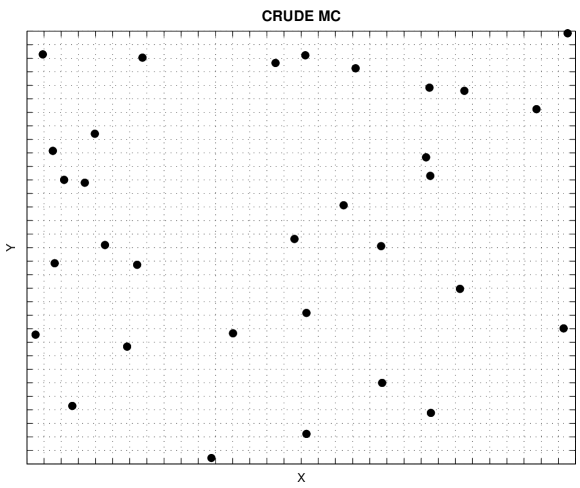
Figure 1: The panel shows 32 points drawn with standard pseudorandom generators

Latin Hypercube Sampling (LHS) can be seen as a way of randomly sampling $n$ points of a stratified sampling while preserving the regularity from stratification (see, for instance, Glasserman [8]). Let $\pi_{1},\dots,\pi_{d}$ be independent random permutations of the first $n$ positive integers, each of them uniformly distributed over the $n!$ possible permutations. Set

$$T_{jk}=\frac{U_{jk}+\pi_{k}\left(j\right)-1}{n},\qquad j=1,\dots,n,k=1,\dots,d,$$ (56)

where $\pi_{k}\left(j\right)$ represents the $j$-th component of the permutation for the $k$-th coordinate. Randomization ensures that each vector $\mathbf{T}_{j}$ is uniformly distributed over the $d$ dimensional hypercube. Moreover, all coordinates are perfectly stratified since there is exactly one sample point in each hypercube of volume $1/n$. For $d=2$, there is only one point in the horizontal or vertical stripes of surface $1/n$ (see Figure 2). The base and the height are $1/n$ and 1, respectively. For $d>2$ it works in the same way. It can be proven that for all $n\geq 2,d\geq 1$ and squared integrable functions $f$, the error for the estimation with the Latin Hypercube Sampling is smaller or equal to the error for the crude Monte Carlo (see Koehler and Owen [15]):

$$Var\left[\widehat{I}_{LHS}\right]\leq\frac{\sigma^{2}}{n-1}.$$ (57)

Figure 2 shows the distribution of 32 points generated with the LHS method. For the LHS method we notice that there is only $1$ point (dotted points in Figure 2) in each vertical or horizontal stripe whose base is $1$ and height is $1/32$: it means that there is only a vertical and horizontal stratification.

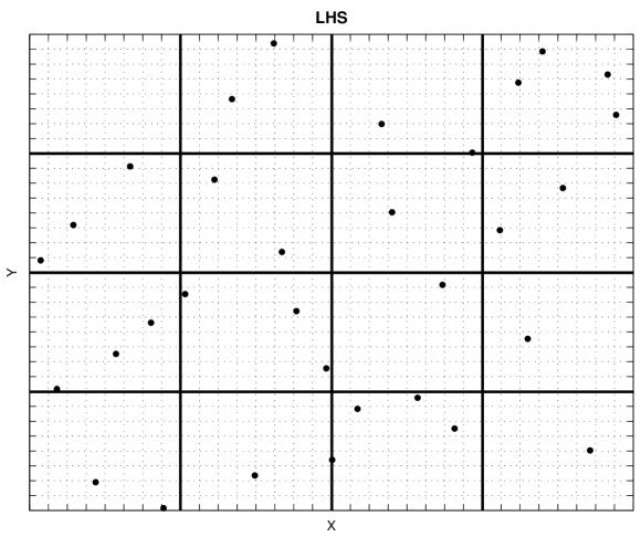
Figure 2: The panel shows 32 points generated with LHS

7.2 Low-Discrepancy Sequences

As previously mentioned, the standard MC method is based on a completely random sampling of the hypercube $\left[0,1\right)^{d}$ and its precision can be improved using stratification or Latin Hypercube sampling. These two methods ensure that there is only one point in each smaller hypercube fixed by the stratification as illustrated in Figure 2. At the same time, these techniques provide nothing more than the generation of uniform random variables in smaller sets.

A completely different way to approach the sampling problem is to build-up a deterministic sequence of points that uniformly covers the hypercube $\left[0,1\right)^{d}$ and to run the estimation using this sequence. Obviously, there is no statistical quantity that may represent the uncertainty since the estimation always gives the same results. The Monte Carlo method implemented with the use of low-discrepancy sequences is called Quasi-Monte Carlo (QMC).

The mathematics involved in generating a low-discrepancy sequence is complex and requires the knowledge of the number theory. In the following, only an overview of the fundamental results and properties is presented (see Niederreiter [17] for more on this issue).

We define the quantity $D_{n}^{\ast}=D_{n}^{\ast}\left(P_{1},\dots,P_{n}\right)$ as the star discrepancy. It is a measure of the uniformity of the sequence $\left\{P_{n}\right\}_{n\in\mathbb{N}^{\ast}}\in\left[0,1\right)^{d}$ and it must be stressed that it is an analytical quantity and not a statistical one. For example, if we consider the uniform distribution in the hypercube $\left[0,1\right)^{d},$ the probability of being in a subset of the hypercube is given by the volume of the subset. The discrepancy measures how the pseudo-random sequence is far from the idealized uniform case, i.e. it is a measure, with respect to the $L_{2}$ norm for instance, of the inhomogeneity of the pseudo-random sequence.

Definition 6 (Low-Discrepancy Sequencies).

A sequence $\left\{P_{n}\right\}_{n\in\mathbb{N}^{\ast}}$ is called low-discrepancy sequence if:

$$D_{n}^{\ast}\left(P_{1},\dots,P_{n}\right)=O\left(\frac{\left(\ln n\right)^{d}}{n}\right).$$ (58)

i.e. if its star discrepancy decreases as $\left(\ln n\right)^{d}/n$.

The following inequality, attributed to Koksma and Hlawka, provides an upper bound to the estimation error of the unknown integral with the QMC method in terms of the star discrepancy:

$$|I-\hat{I}|\leq D_{n}^{\ast}\,\,V_{HK}\left(f\right).$$ (59)

$V_{HK}\left(f\right)$ is the variation in the sense of Hardy and Krause. Consequently, if $f$ has a finite variation and $n$ is large enough, the QMC approach gives an error smaller than the error obtained by the crude MC method for low dimensions $d$. However, the problem is difficult owing to the complexity if estimating the Hardy-Krause variation, which depends on the particular integrand function.

In the following sections we briefly present digital nets and the well-known Sobol’ sequence that is the most frequently used low discrepancy sequence to run Quasi-Monte Carlo simulations in finance.

7.3 Digital Nets

Digital nets or sequences are obtained by the number theory and owe their name to the fact that their properties can be recognized by their digital $b$-ary expansion in base $b$. Many digital nets exist; the ones most often used and considered most efficient are the Sobol’ and the Niederreiter-Xing sequences.

The first and simplest digital sequence with $d=1$ is due to Van der Corput and is called the radical inverse sequence. Given an integer $b\geq 2$, any non-negative number $n$ can be written in base $b\$as:

$$n=\sum_{k=1}^{\infty}n_{k}b^{k-1}.$$ (60)

The base $b$ radical inverse function $\phi_{b}\left(n\right)$ is defined as:

$$\phi_{b}\left(n\right)=\sum_{k=1}^{\infty}n_{k}b^{-k}\quad\in\left[0,1\right),$$ (61)

where $n_{k}\in\left\{0,1,\dots,b-1\right\}$ (Galois set).

By varying $n$ the Van der Corput sequence is constructed.

$N$	$n$ base 2	$\phi_{2}\left(n\right)$ base 2	$\phi_{2}\left(n\right)$
0	000.	0.000	0.000
1	001.	0.100	0.500
2	010.	0.010	0.250
3	011.	0.110	0.750
4	100.	0.001	0.125
5	101.	0.101	0.625
6	110.	0.011	0.375
7	111.	0.111	0.875

Table 1: Van der Corput sequence.

Table 1 illustrates the first seven Van der Corput points for $b=2$. Consecutive integers alternate between odd and even; these points alternate between values in $\left[0,1/2\right)$ and $\left[1/2,1\right)$. The peculiarity of this net is that any consecutive $b^{m}$ points from the radical inverse sequence in base $b$ are stratified with respect to $b^{m}$ congruent intervals of length $b^{-m}$. This means that in each interval of length $b^{-m}$ there is only one point.

Table 1 shows an important property that is exploited in order to generate digital nets, because a computing machine can represent each number with a given precision, referred to as “machine epsilon”. Let $z=0.z_{1}z_{2}\dots(base$ $b)\in\left[0,1\right)$ , define $\mathbf{\Psi}(z)=(z_{1},z_{2},\dots)$ the vector of the its digits, and truncate its digital expansion at the maximum allowed digit $w$: $z=\sum_{k=1}^{\emph{w}}z_{k}b^{-k}$. Let $n=\left[b^{w}z\right]=\sum_{h=1}^{w}n_{h}b^{h-1}\in N^{\ast}$, where $\left[x\right]$ denotes the greatest integer less than or equal to $x$. It can be easily proven that:

$$n_{h}=z_{w-h+1}\left(z\right)\quad\forall h=1,\dots,w.$$

This means that the finite sequences $\left\{n_{h}\right\}_{h\in\left\{1,\dots,w\right\}}$ and $\left\{z_{k}\right\}_{k\in\left\{1,\dots,w\right\}}$ have the same elements in opposite order. For example, in the table 1 we allow only $3$ digits; in order to find the digits of $\phi_{2}\left(1\right)=0,5$ we consider $\phi_{2}\left(1\right)2^{3}=4=0n_{1}+n_{2}0+n_{3}1$. The digits of $\phi_{2}\left(1\right)$ are then $(1,0,0)$ as shown in the table 1.

The peculiarity of the Van der Corput sequence is largely required in high dimensions, where the contiguous intervals are replaced by multi-dimensional sets called b-adic boxes.

Definition 7 (b-iadic Box).

Let $b\geq 2$, $k_{j}$, $l_{j}$ with $0\leq l_{j}\leq b^{k_{j}}$ be all integer numbers. The following set is called b-iadic box:

$$\prod_{j=1}^{d}\left[\frac{l_{j}}{b^{k_{j}}},\frac{l_{j}+1}{b^{k_{j}}}\right),$$ (62)

where the product represents the Cartesian product.

Definition 8 ((t,m,d) Nets).

Let $t\leq m$ be a non-negative integer. A finite set of points from $\left[0,1\right)^{d}$ is called $\left(t,m,d\right)$-net if every b-adic box of volume $b^{-m+t}$ (bigger than $b^{-m}$) contains exactly $b^{t}$ points.

This means that cells that “should have” $b^{t}$ points do have $b^{t}$ points. However, considering the smaller portion of volume $b^{-m}$, it is not guaranteed that there is just one point.

A famous result of the theory of digital nets is that the integration over a $\left(t,m,d\right)$ net can attain an accuracy of the order of $O\left(\ln^{d-1}\left(n\right)/n\right)$ while, restricting to $\left(t,d\right)$ sequences, it raises slightly to $O\left(\ln^{d}\left(n\right)/n\right)$ (see Niederreiter [17]). The above results are true only for functions with bounded variation in the sense of Hardy-Krause.

7.4 The Sobol’ Sequence

The Sobol’ sequence is the first $d$ dimensional digital sequence, ($b=2$), ever realized. Its definition is complex and is covered only briefly in the following.

Definition 9 (The Sobol’ Sequence).

Let $\left\{n_{k}\right\}_{k\in\mathbb{N^{\ast}}}$ be the set of the b-ary expansion in base $b=2$ of any integer $n$; the $n$-th element $S_{n}$ of the Sobol’ sequence is defined as:

$$S_{n}=\sum_{k=1}^{+\infty}\left(n_{k}\,V_{k}\,mod\,2\right)\,2^{-k},$$ (63)

d	P	M	Principal polynomial	q
1	[1]	[1]	$1$	0
2	[1 1]	[1]	$x+1$	1
3	[1 1 1]	[1 1]	$x^{2}+x+1$	2
4	[1 0 1 1]	[1 3 7]	$x^{3}+x+1$	3
5	[1 1 0 1]	[1 1 5]	$x^{3}+x^{2}+1$	3
6	[1 0 0 1 1]	[1 3 1 1]	$x^{4}+x+1$	4
7	[1 1 0 0 1 ]	[1 1 3 7]	$x^{4}+x^{3}+1$	4
8	[1 0 0 1 0 1]	[1 3 3 9 9]	$x^{5}+x^{2}+1$	5
9	[1 1 1 0 1 1]	[1 3 7 13 3]	$x^{5}+x^{4}+x^{3}+x+1$	5
10	[1 0 1 1 1 1]	[1 1 5 11 27]	$x^{5}+x^{3}+x^{2}+x+1$	5

Table 2: Initial values satisfying Sobol property A up to dimension 10. By convention, the recurrence relation for the $0$-degree polynomial is $M_{k}\equiv 1$

where $V_{k}\in\left[0,1\right)^{d}$ are called direction numbers. In practice, the maximum number of digits, $w$, must be given. In Sobol’s original method the $i$-th number of the sequence $S_{ij}$, $i\in{\mathbb{N}},j\in\left\{1,\dots,d\right\}$, is generated by XORing (bitwise exclusive OR) together the set of $V_{kj}$ satisfying the criterion on $k$ : the $k$-th bit of $i$ is nonzero. Antonov and Saleev derived a faster algorithm by using the Grey code. Dropping the index $j$ for simplicity, the new method allows us to compute the $\left(i+1\right)$-th Sobol’ number from the $i$-th by XORing it with a single $V_{k}$, namely with $k$, the position of the rightmost zero bit in $i$ (see, for instance, Press, Teukolsky, Vetterling and Flannery [23]). Each different Sobol’ sequence is based on a different primitive polynomial over the integers modulo 2, or in other words, a polynomial whose coefficients are either 0 or 1. Suppose $P$ is such a polynomial of degree $q$:

$$P=x^{q}+a_{1}x^{q-1}+a_{2}x^{q-2}+\dots+a_{q-1}x+1.$$ (64)

Define a sequence of integers $M_{k}$, by the $q$th term recurrence relation:

$$M_{k}=2a_{1}M_{k-1}\oplus 2^{2}a_{2}M_{k-2}\oplus\dots\oplus 2^{q-1}M_{k-q+1}a_{q-1}\oplus\left(2^{q}M_{k-q}\oplus M_{k-q}\right).$$ (65)

Here $\oplus$ denotes the XOR operation. The starting values for the recurrence are $M_{1},\dots,M_{q}$ that are odd integers chosen arbitrarily and less than $2,\dots,2^{q}$, respectively. The directional numbers $V_{k}$ are given by:

$$V_{k}=\frac{M_{k}}{2^{k}}\qquad k=1,\dots,w.$$ (66)

Table 2 shows the first ten primitive polynomials and the starting values used to generate the direction numbers for the $10$ dimensional Sobol’ sequence.

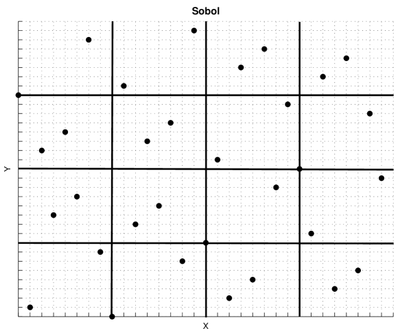
Figure 3: The panel shows the first 32 points of the 2-dimensional Sobol’ sequence

7.5 Scrambling Techniques

Digital nets are deterministic sequences. Their properties ensure good distribution in the hypercube $\left[0,1\right)^{d}$, enabling precise sampling of all random variables, even if they are very skewed. The main problem is the computation of the error in the estimation, since it is difficult to compute and depends on the chosen integrand function. To review, the crude MC provides an estimation with low convergence independent of $d$ and the possibility to statistically evaluate the RMSE. On the other hand, the QMC method gives a higher convergence, but there is no way to statistically calculate the error.

In order to estimate a statical measure of the error of the Quasi-Monte Carlo method we need to randomize a $\left(t,m,d\right)$-net and try to obtain a new version of points such that it still is a $\left(t,m,d\right)$-net and has uniform distribution in $\left[0,1\right)^{d}$.

This randomizing procedure is called scrambling. The scrambling technique permutes the digits of the digital sequence and returns a new sequence that has both the properties described above.

The scrambling technique we use is called Faure-Tezuka Scrambling (for a precise description see Owen [21], Hong and Hickernell [10]).

For any $z\in\left[0,1\right)$ we define $\mathbf{\Psi}(z)$ as the $\infty\times 1$ vector of the digits of $z$.

Now let $L_{1},\dots L_{d}$ be nonsingular lower triangular $\infty\times\infty$ matrices and let $\mathbf{e_{1}},\dots,\mathbf{e_{d}}$ be $\infty\times 1$ vectors. Only the diagonal elements of $L_{1},\dots L_{d}$ are chosen randomly and uniformly in $Z_{b}^{\ast}=\left\{1,\dots,b\right\}$ , while the other elements are chosen in $Z_{b}=\left\{0,1,\dots,b\right\}$. $\mathbf{Y}$, the Faure-Tezuka scrambling version of $\mathbf{X}$, is defined as:

$$\mathbf{\Psi}\left(y_{ij}\right)=\left(L_{j}\,\mathbf{\Psi}\left(x_{ij}\right)+\mathbf{e}_{j}\right)modb$$ (67)

All operations take place in the finite field $Z_{b}$. Owen proved that, with his scrambling, it is possible to obtain (see Owen [18]):

$$Var\left[\hat{I}\right]\leq\frac{b^{t}}{n}\left[\frac{b+1}{b-1}\right)^{d}\sigma^{2},$$ (68)

for any twice integrable function in $\left[0,1\right)^{d}$. These results state that for low dimension $d$ , the randomized QMC (RQMC) provides a better estimation with respect to Monte Carlo, at least for large $n$.

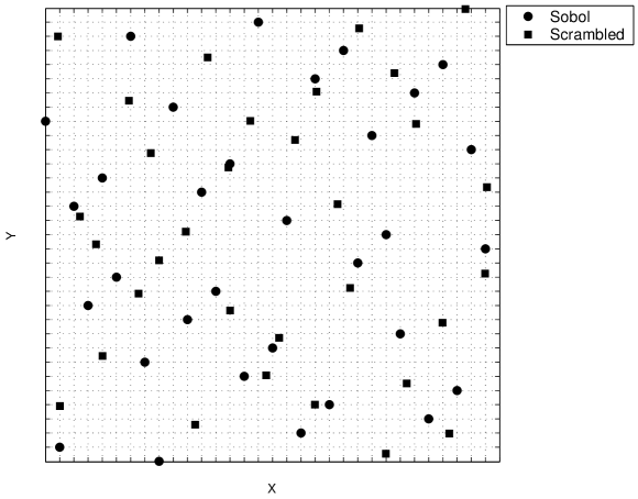
Figure 4: The panel shows the first 32 point of the Sobol sequence compared to their Faure-Tezuka scrambled version

8 Implementation and Algorithm

We illustrate the simulation procedure to compute the arithmetic Asian option price. The purpose of our analysis is to characterize the efficiency of Monte Carlo methods based on the path generation techniques and the uniform points used for the evaluation of the integral (23). We consider separately the constant volatility and time-dependent volatility markets.

It must be stressed that Quasi-Monte Carlo estimations are dramatically influenced by the problem dimension, because the rate of convergence depends on the problem dimension $d$, as it can be seen in equations (58) and (68). Many studies and experiments suggest that Quasi-Monte Carlo methods can only be used for problem dimensions up to $20$ (see Boyle, Broadie and Glasserman [2] for more on this issue). This condition translates into a relationship between the number $M$ of underlying assets and the number $N$ of monitoring times: $M\times N\leq 20$. When this condition is not satisfied anymore we use the Latin Supercube method that we describe hereafter.

8.1 Latin Supercube Sampling

The scrambling procedure allows the statistical estimation of the RMSE as the crude MC does with the order of convergence that depends on the the dimension $d$. For high $d$ the fast convergence of the RQMC is lost, there is no benefit to use it compared to the simple MC. Generally in finance the dimension is high even using dimension reduction techniques like ANOVA-PCA decomposition.
Owen [20] has proposed a method to extend the convenience of applicability of RQMC for high dimensions. This method is called Latin Supercube Sampling, (LSS), owing to its similarity to the LHS. The random permutation is now applied to a set of subsequence of the original one with some statistical sense.
Let $\mathbf{Y}=\{\mathbf{y_{1}},\dots,\mathbf{y_{b^{m}}\}}$ be the digital sequence of the simulation variables, and ${b^{m}}=N$. Dividing it into $k$ nonempty and disjoint subsets $\mathbf{Y}=\bigcup_{r=1}^{k}\mathbf{Y_{r}}$ and letting $s_{r}=dim\mathbf{Y_{r}}$ we have $\sum_{r=1}^{k}s_{r}=d$. In practice, each point of the sequence can be represented as $\mathbf{y_{i}}=(\chi_{i}^{1},\dots,\chi_{i}^{k})$, where $\chi_{i}^{r}\in[0,1[^{s_{r}}$; these points $\chi_{i}^{r}$ are ordinarily points of an $s_{r}$-dimensional RQMC method.
For $r=1,\dots,k$ let $\pi_{r}(i)$ be an independent uniform and random permutation of $\{1,\dots,N\}$ than a Latin Supercube sample is obtained by taking:

$$\mathbf{\hat{y}_{i}}=(\chi_{\pi_{1}(i)}^{1},\dots,\chi_{\pi_{k}(i)}^{k})$$ (69)

It means that the first $s_{1}$ colums in the LSS are obtained by randomly permuting the run order of the RQMC points $\chi_{i}^{1},\dots,\chi_{i}^{1}$, the next $s_{2}$ columns come from an independent permutation of the run order of $\chi_{i}^{2}$ and so on.

The convenient way to divide the original set might be arranging them in statistically orthogonal sets using the ANOVA-PCA decomposition.

In practice in financial simulation with $d$ Brownian motions, it may make sense to select $5$ principal components of each path, to apply an RQMC method to each of them with LSS and then pad them out the other variables with LHS. In fact, about $95\%$ of the total variance of the Brownian motion is explained by these components. Alternatively, it may be better to group the first $k$ principal component, then the second, and so on.

However, all these results are weak and only the practical test can give an answer to which sequence and scrambling should be used.

8.2 Key Steps of the Simulation Procedure

As a first scenario we run simulations using the Cholesky and the PCA decomposition procedures for the constant volatility case. As a second scenario we test the efficiency of the proposed Kronecker product approximation by comparing the its results with those obtained with the PCA decomposition.

As a random number generator we use three configurations: standard, LHS and Faure-Tezuka scrambled version of the Sobol’ sequence.

The test for constant volatility consists of three main steps:

1. Random number generation by standard MC, LHS or RQMC.

2. Path generation with Cholesky and PCA decompositions.

3. Monte Carlo estimation.

For the time-dependent volatility case the three steps are:

1. Random number generation by RQMC.

2. Path generation with PCA decomposition and KPA.

3. Monte Carlo estimation.

The first step of both cases is realized by using the correspondent random generator of uniform random variables. In order to extract normal random variables we rely on the inverse transform method that require the numerical inversion of the cumulative function of the standard normal. This numerical procedure may destroy the better stratification and the uniformity introduced by LHS and especially by low-discrepancy sequences. We use the Moro’s algorithm that is more precise than the standard one due to Beasley and Springer. It provides a better accuracy on the tails of the inverse normal where we require that the LHS and Sobol sequences must reveal their higher precision, see Moro [16] and Glasserman [8] for more on the topic.

For constant volatilities the second step can be implemented by the following algorithm:

1. Define the parameters of the simulation.

2. Define the drift as in equation (20).

3. Create the $N\times N$ correlation matrix $\left(R\right)_{l,k}=\left(t_{l}\wedge t_{k}\right);l,k=1,\dots,N$.

4. Define the correlation matrix $\Sigma$ among the $M$ asset returns.

5. Perform either a PCA or the Cholesky decomposition on the global correlation matrix $\Sigma_{MN}$. This matrix is built up by repeating the constant block of correlation $\Sigma$ at all the times of observation.

For time-depending volatilities we define the drift as equation (21), while the last operation consists of performing the PCA decomposition and the KPA.

Stratification introduces a correlation among random drawings so that the hypothesis of the Central Limit theorem is not satisfied and we cannot compute the RMSE straightforward. We rely on the batch method that consists of repeating $N_{B}$ simulations for $B$ times (batches). We assume that each of the $B$ batches eliminates the correlation and the results form a sequence of $B$ independent random variables. We compute the average Asian price for each batch; the RMSE becomes:

$$RMSE=\sqrt{\frac{\sum_{b=1}^{B}\left(\bar{a}\left(0\right)_{b}-\bar{a}\left(0\right)\right)^{2}}{B\left(B-1\right)}},$$ (70)

where $\left(\bar{a}\left(0\right)_{1},\dots,\bar{a}\left(0\right)_{B}\right)$ is a sample of the average present values of the Asian option generated in each batch.

9 Numerical Experiments

We perform a test of all the valuation procedures described in the previous section. We specify our investigation into constant and time-dependent volatilities cases while our experiments involve standard Monte Carlo, the Latin Hypercube Sampling and Randomized Quasi Monte Carlo with the Faure-Tezuka scrambled version of the Sobol’ sequences.

9.1 Constant Volatility: Results

As for a first pricing experiment we consider an at-the-money arithmetic Asian option with strike price $K=100$, written on a basket of $M=2$ underlying assets, expiring at $T=1$ year and sampled $N=5$ times during its lifetime.

All results are obtained by using $S=8192$ drawings and $10$ replications. Table 3 reports the input parameters for our test.

$\begin{array}[]{lll}S_{i}\left(0\right)&=&100\\ K&=&100\\ r&=&2\%\\ T&=&1\\ \sigma_{1}&=&30\%\\ \sigma_{2}&=&40\%\\ \rho_{ij}&=&0\text{ and }40\%\quad\text{for }i,j=1,2.\end{array}$

Table 3: Input Parameters Used in the First Simulation

The nominal dimension of the problem is $M\times N=10$ that is equal to the number of rows and columns of the global correlation matrix $\Sigma_{MN}$. Paths are simulated by using both PCA and the Cholesky decomposition as in Dahl and Benth [6] and [7].

Table 4 and Table 5 show the results for the positive correlation and uncorrelated cases, respectively. Simulated prices of the Asian basket options are in statistical accordance, while the estimated RMSEs depend on the sampling strategy adopted. The rate of convergence of the RQMC estimation is higher than the other two methods. In particular it is ten times higher than the standard Monte Carlo method that would return the same accuracy with $100\times S$ drawings.

We observe that the PCA generation provides a better estimation both for LHS and RQMC, because these ones are more sensitive to the effective dimension, while PCA causes no distinction for the standard MC. The effect is more pronounced for the correlation case where the more complex structure of the global correlation matrix $\Sigma_{MN}$ influences the estimation procedure.

As from a financial perspective, it is normal to find a higher price in the positive correlation case than in the uncorrelated one.

	Standard MC	LHS	RQMC
PCA	7.195 (0.016)	7.157 (0.013)	7.1696 (0.0017)
Cholesky	7.242 (0.047)	7.179 (0.022)	7.1689 (0.0071)

Table 4: Uncorrelation Case. Estimated Prices and Standard Errors.

	Standard MC	LHS	RQMC
PCA	8.291 (0.053)	8.2868 (0.0073)	8.2831 (0.0016)
Cholesky	8.374 (0.055)	8.293 (0.026)	8.2807 (0.0064)

Table 5: Correlation Case. Estimated Prices and Standard Errors.

Moreover, we develop our analysis by investigating a very high-dimensional pricing problem. A basket of $M=10$ underlying assets is considered with $N=250$ sampling time points, the nominal dimension is $d=2500$.

We run our simulation with the same parameters used by Imai and Tan [11] and use the LSS for the high-dimensional QMC estimation as presented in the cited reference. The authors concatenated 100 or 50 sets of 25 or 50 dimensional Sobol’ sequence, respectively. They exploit the LSS method in order to obtain a complete 2500 dimensional sample of digital net. Owen [19] is more restrictive; the author suggests to use scrambled digital sequences for the first five or ten components and LHS for the others or to concatenate the principal components. We compare the results and investigate the effective dimensions and the contribution of the eigenvalues of the global correlation matrix. Table 6 reports input parameters for our test.

$\begin{array}[]{lll}S_{i}\left(0\right)&=&100\\ K&=&100\\ r&=&4\%\\ T&=&1\\ \sigma_{i}&=&10\%+\frac{i-1}{9}40\%\quad\text{for }i=1,\dots,10\\ \rho_{ij}&=&0\quad\textrm{and}\quad 40\%\quad\text{for }i,j=1,\dots,10\end{array}$

Table 6: Input Parameters Used in the Second Simulation

We compute the eigenvalues and eigenvectors of $\Sigma_{MN}$. Property (10) of the Kronecker product is fundamental in this computation and considerably reduces the computational burden and time. It results that the effective dimension is $143$ or $170$ for the correlation and uncorrelation cases, respectively, are much smaller than the nominal one. Considering the first $143$($170$) columns, that is the first $143$($170$) principal components, the generating matrix $C$ takes into account $99\%$ of the total variance.

Table 7 shows all the results we obtained. We concatenate $50$ sets of $50$-dimensional randomized low-discrepancy sequences.

Uncorrelation	Standard MC	LHS	RQMC
PCA	3.414(0.015)	3.4546(0.0054)	3.4438(0.0015)
Cholesky	3.426(0.015)	3.4323(0.0070)	3.4518(0.0058)
Correlation	Standard MC	LHS	RQMC
PCA	5.648(0.029)	5.6655(0.0032)	5.65750(0.00040)
Cholesky	5.604(0.029)	5.670(0.013)	5.63710(0.019)

Table 7: Prices and RMSEs both for the correlated and uncorrelated case when $100\%$ of the variance is considered.

We consider both the matrix of $2500$ rows and $143$($170$) columns, excluding the effects of the remaining principal components, and the complete ANOVA in order to investigate the effectiveness of our assumptions and hypotheses.

Table 8 presents the different Monte Carlo estimations with respect to the number of eigenvalues when LHS is used.

	Positive Correlation			Zero Correlation
Price	RMSE	E	Price	RMSE	E
5.262	0.090	5	2.596	0.041	5
5.294	0.088	10	3.190	0.047	10
5.433	0.088	15	3.212	0.047	15
5.528	0.091	20	3.239	0.047	20
5.484	0.092	25	3.289	0.047	25
5.445	0.090	30	3.375	0.048	30
5.653	0.015	147	3.452	0.010	170

Table 8: Prices and RMSE for different principal components when LHS is used.

Uncorrelation	RQMC	Correlation	RQMC
PCA	3.4475(0.0023)	PCA	5.65860(0.00072)
Cholesky	3.426(0.0087)	Cholesky	5.603(0.022)
LT	3.4461(0.0012)	LT	5.6780(0.00047)

Table 9: Estimated Results by Imai and Tan [13]

Table 9 illustrates the values found by Imai and Tan [11]. Their results were obtained assigning the importance of each component (not anymore PCA) with their LT method. All the estimations found are unbiased and in agreement with those presented in the cited references.

The Quasi-Monte Carlo method with LSS extension proves to be a powerful variance reduction technique, particularly when coupled with the ANOVA-PCA decomposition. Moreover, the Kronecker product turns out to be a fast tool to generate multi-dimensional Brownian paths. Indeed, the elapsed time to realize the same path without using the properties of the Kronecker product is a lot higher.

The estimation with Cholesky decomposition gives higher uncertainty than the PCA approach, meaning that a small amount of variance is lost. This is due to the fact that a relevant part of the variance is carried out by a few eigenvalues of the covariance matrix $R$. If these eigenvalues are observed, it can be noticed that only few of them are relevant in the PCA analysis and they are much bigger than the ones of the matrix $\Sigma$.

9.2 Constant Volatility: Comments

Based on these results, we can make the following conclusions:

1. The RQMC method and the use of the Faure-Tezuka scrambling technique provide the best estimation among all the implemented procedures for both the “Correlation” and “Zero Correlation” cases. The correspondent RMSEs are the smallest ones with a higher order of convergence with the same number of simulations.

2. The Kronecker product is a fast and efficient tool for generating multi-dimensional Brownian paths with a low computational effort.

3. As compared to to the standard Monte Carlo and LHS approaches, the use of scrambled low-discrepancy sequences provides more accurate results, at least for $M\times N\leq 20$, particularly with the PCA and LT-based methods.

4. The accuracy of the estimates is strongly dependent on the choice of the Cholesky or the PCA approach. In particular, independent of the simulation procedure (MC, LHS or RQMC), when using PCA decomposition the estimates are affected by a smaller sampling error (smaller standard error).

9.3 Time-dependent Volatility: Results

The constant volatility hypothesis is the starting point for the pricing problem. A further improvement can be achieved by considering a time-dependent volatility function.

It is market practice to choose step-wise time-dependent volatilities. We want to investigate a more complex dependence to test our new approach based on the Kronecker product approximation. For this aim, we adopt an exponentially decaying function having the following expression:

$$\sigma_{i}=\hat{\sigma}_{i}(0)\,exp\big{(}-\frac{t}{\tau_{i}}\big{)}+\sigma_{i}(+\infty)$$ (71)

where $\hat{\sigma}_{i}(0)+\sigma_{i}(+\infty)=\sigma_{i}(0)$ is the initial volatility for the $i$-th asset, $\sigma_{i}(+\infty)$ is its asymptotic volatility and $\tau_{i}$ its decay constant.

The particular time-dependent function leads to the following solution:

$$\int_{0}^{t_{j}\wedge t_{l}}\sigma_{i}(t)\sigma_{k}(t)\rho_{ik}dt = \hat{\sigma}_{i}(0)\hat{\sigma}_{k}(0)\tau_{ik}\Big{(}1-exp\big{(}-\frac{t}{\tau_{ik}}\big{)}\Big{)}+$$

$$+\hat{\sigma}_{i}(0)\sigma_{k}(+\infty)\tau_{i}\Big{(}1-exp\big{(}-\frac{t}{\tau_{i}}\big{)}\Big{)}+$$

$$+\hat{\sigma}_{k}(0)\sigma_{i}(+\infty)\tau_{ik}\Big{(}1-exp\big{(}-\frac{t}{\tau_{ik}}\big{)}\Big{)}+$$

$$+\sigma_{i}(+\infty)\sigma_{k}(+\infty)t$$

where $\tau_{ik}=\tau_{i}\tau_{k}/(\tau_{i}+\tau_{k})$.

The simulation implemented to obtain the price of an Asian option supposing time-dependent volatility evolves as the constant volatility case. The main difference is the procedure to reduce the dimension of the problem.

The parameters chosen for the simulation are listed in table 10.

$\begin{array}[]{lll}S_{i}(0)&=&100\\ r&=&4\%\\ T&=&1\textrm{year}\\ \sigma_{i}(0)&=&10\%+\frac{i-1}{9}40\%\\ \sigma_{i}(+\infty)&=&9\%\qquad\textrm{for all i}\\ \tau_{i}&=&1.5\textrm{year}\\ K&=&100\\ \rho_{ij}&=&0\quad\textrm{and}\quad 40\%\quad\textrm{for}\quad i,j=1,\dots,10\end{array}$

Table 10: Input Parameters for the Time-depending Case

The initial volatilities are equal to those used in the constant volatility case. The asymptotic volatility and the decay constant are the same among all the assets. These parameters are chosen in order to allow a comparison with respect to the constant volatility case. Indeed, the price of the options is sensitive to the change of volatility and in particular its decreasing trend should provide a lower price.

The basket consists of $10$ underlying assets, the time grid has $250$ equally spaced points and the number of runs is $S=8192$ and $10$ replications. Table 11 shows the results coming from the simulation using the RQMC method both with the KPA and the PCA for dimension reduction.

Positive Correlation (KPA)		Zero Correlation(KPA)
Price	5.19658	Price	3.20784
RMSE	0.00063	RMSE	0.00040
E	145	E	173
Positive Correlation (PCA)		Zero Correlation(PCA)
Price	5.19856	Price	3.20147
RMSE	0.00062	RMSE	0.00040
E	123	E	150

Table 11: Estimated Results for the Time-depending Case, ANOVA = 0.99

The KPA path-generation is efficient and fast. To have an idea of its speed, the elapsed times to obtain the generating matrix without exploiting the properties of the Kronecker product and no approximations are more than ten times higher. As expected, the simulation gives smaller prices with respect to the constant volatility situation, because a decreasing volatility function has been assigned.

The nominal dimensions of the problem $E$ using PCA come out to be $126$ and $150$ for the correlation and uncorrelation cases. When adopting the KPA the approximated nominal dimensions are higher, $145$ and $173$, respectively. If we would consider ANOVA $=0.9885$ for the correlation case and ANOVA = $0.98805$ for the uncorrelation case we would get the PCA-found nominal dimension for ANOVA=$0.99$. We can judge this small difference as negligible and consequently our approximating technique to be efficient and leading to consistent results. As with $N$ and $M$ small, the Cholesky decomposition alone would require a small number of operations without giving any order of the importance for the random sources.

	KPA	PCA	Cholesky
Price	3.20545	3.20390	3.1838
RMSE	0.00040	0.00041	0.0091

Table 12: Uncorrelation Case. Estimated Prices and Standard Errors. ANOVA$=1$.

	KPA	PCA	Cholesky
Price	5.20060	5.20210	5.1946
RMSE	0.00050	0.00058	0.0093

Table 13: Correlation Case. Estimated Prices and Standard Errors. ANOVA$=1$.

Tables 12 and 13 present the estimated prices when taking into account the full components. All the results are in accordance with those ones found with ANOVA$=0.99$.

Table 14 illustrates the sensitivity with respect to the number of principal components $E$:

	Positive Correlation			Zero Correlation
Price	RMSE	E	Price	RMSE	E
5.7805	0.0079	5	2.6368	0.0038	5
4.9904	0.0081	10	2.9681	0.0042	10
5.0226	0.0081	15	3.1172	0.0043	15
5.1103	0.0081	20	3.0979	0.0043	20
5.1826	0.0083	25	3.1051	0.0043	25
5.1937	0.0082	30	3.1514	0.0043	30

Table 14: Prices and RMSEs for different principal components. Case: RQMC

As in the constant volatility case it can be seen that the estimation is convergent.

Moreover, we launch a new simulation with the LHS technique with the same set of parameters. We list the estimated results in table 15.

	Positive Correlation			Zero Correlation
Price	RMSE	E	Price	RMSE	E
4.874	0.016	5	3.121	0.089	5
5.093	0.016	10	3.118	0.085	10
5.097	0.016	15	3.122	0.086	15
5.131	0.016	20	3.072	0.086	20
5.145	0.016	25	3.163	0.088	25
5.201	0.016	30	3.110	0.089	30

Table 15: Prices and RMSEs for different principal components. Case: LHS

The estimated prices have higher RMSEs, confirming the fact that the RQMC approach provides a good variance reduction.

9.4 Time-Dependent Volatility: Comments

According to the results we have found in the time-dependent case, it is possible to draw the following conclusions:

1. RQMC with LSS is a general approach that does not depend on the chosen price dynamic.

2. The KPA we propose, provides unbiased estimations with a reduction of the computational cost. In the framework we investigate, KPA returns a higher nominal dimension, as expected, but only relatively to a negligible amount of variance.

3. KPA is a lot faster than the straightforward PCA because it exploits the properties of the Kronecker product and the boomerang shaped matrices. The ad hoc Cholesky decomposition algorithm we develop is fundamental for the KPA. We do not report computational times because we expect that further improvements can be done.

4. KPA and PCA can be considered both valid as path-generation methods to support the ANOVA and the identifications of effective dimensions.

References

- [1] P. Acworth, M. Broadie, and P. Glasserman. 1998. A comparison of some Monte Carlo and quasi-Monte Carlo methods for option pricing. In Monte Carlo and Quasi-Monte Carlo Methods 1996: Proceedings of a conference at the University of Salzburg, Austria, July 9-12, 1996, ed. H. Niederreiter, P. Hellekalek, G. Larcher and P. Zinterhof. Lecture Notes in Statistics 127. Springer-Verlag, New York.
- [2] P. Boyle, M. Broadie and P. Glasserman. 1995. Recent Advances in Simulation for Security Pricing. Proceedings of the 1995 Winter Simulation Conference. C. Alexopoulos, K. Kang, W.R. Lilegdon and D. Goldsman,ed.s.
- [3] P. Boyle, M. Broadie and P. Glasserman. 1997. Monte Carlo Methods for Security Pricing. Journal of Economics Dynamics and Control. 21: 1267-1321
- [4] R. Caflisch, W. Morokoff, and A. Owen. 1997. Valuation of mortgage-backed securities using Brownian bridges to reduce effective dimension. Journal of Computational Finance 1 (1):27 46.
- [5] N. Cufaro-Petroni. 1996. Lezioni di Calcolo delle Probabilità. Edizioni dal Sud. Modugno. 1996.
- [6] L.O. Dahl, F.E. Benth. 2001. Valuation of the Asian Basket Option with Quasi-Monte Carlo Techniques and Singular Value Decomposition. Pure Mathematics. 5.
- [7] L.O. Dahl, F.E. Benth. 2002. Fast Evaluation of the Asian Option by Singular Value Decomposition. Proceedings of the Conference: Monte Carlo and Quasi-Monte Carlo Methods 2000. K.-T. Fang, F.J.Hickernell, H. Niederreiter,ed.s. 201-214, Springer-Verlag Berlin Heidelberg 2002.
- [8] P. Glasserman. 2004. Monte Carlo Methods in Financial Engineering. Springer-Verlag New York. 2004.
- [9] G.H. Golub, C.F. Van Loan. 1996. Matrix Computations 3rd Ed. The Johns Hopkins University Press 1996.
- [10] H.S. Hong, F.J. Hickernell. 2000. Implementing Scrambled Digital Nets. Unpublished Technical Report, Hong Kong Baptist University.
- [11] J. Imai, K.S. Tan. 2002. Enhanced Quasi-Monte Carlo Method with Dimension Reduction. Proceedings of the 2002 Winter Simulation Conference. D.J. Medeiros, E. Y cesan,C.-H. Chen, J.L. Snowdon and J.M. Charnes,ed.s.
- [12] J. Imai, K.S. Tan. 2005. Minimizing Effective Dimension using Linear Transformation. Monte Carlo and Quasi-Monte Carlo Methods 2004. H. Niederreiter editor, Springer-Verlag 2005.
- [13] J. Imai, K.S. Tan. 2007. A General Dimension Reduction Technique for Derivative Pricing. Journal of Computational Finance. Volume 10/Number 2. Winter 2006/2007. Pages 129-155.
- [14] A.N. Langville, W.J. Stewart. 2004. The Kronecker Products and Stochastic Automata Networks. Journal of Computational and Applied Mathematics Volume 167, Issue 2, 1 June 2004, Pages 429-447
- [15] J.R. Koehler, A. Owen. 1996. Computer Experiment. Handbook of Statistics. Design and Analysis of Experiments. S. Ghosh and C.R. Rao,ed.s.
- [16] B. Moro. 1995. The Full Monte. Risk(8)(Feb):57-58.
- [17] H. Niederreiter. 1992. Random Number Generation and Quasi-Monte Carlo Methods. S.I.A.M., Philadelphia 1992.
- [18] A. Owen. 2003. Quasi-Monte Carlo Sampling. Chapter for a SIGGRAPH 2003 course. San Diego.
- [19] A. Owen. 1998. Monte Carlo Estension of Quasi-Monte Carlo. Proceedings of the 1998 Winter Simulation Conference. D.J. Medeiros, E.F. Watson, J.S. Carson and M.S. Manivannan,ed.s.
- [20] A. Owen. 1998. Latin Supercube Sampling for Very High-dimensional Simulations. ACM Transaction on Modelling and Computer Simulation. 8: 71-102.
- [21] A. Owen. 2002. Variance and Discrepancy with Alternative Scramblings. ACM Transactions on Computational Logic, Vol V.
- [22] N. Pitsianis, C.F. Van Loan. 1993. Approximation with Kronecker Products. Linear Algebra for Large Scale and Real Time application. M.S. Moonen and G.H. Golub, ed.s. Kluwer Academic Publishers, 293-314.
- [23] W.H. Press, S.A. Teukolsky, W.T. Vetterling, B.P. Flannery. 1992. Numerical Recipes in C: the Art of Technical Computing. Cambridge University Press.
- [24] R. Rebonato. 2004. Volatility and Correlation or the Perfect Hedger and the Fox. John Wiley & Sons 2004.
- [25] C.F. Van Loan. 2000. The Ubiquitous Kronecker Product. Journal of Computational and Applied Mathematics. 123: 85-100.
- [26] J. Veĉer. 2001. A new PDE approach for pricing arithmetic average Asian options. Journal of Computational Finance, Vol. 4, No. 4, 105-113.
- [27] J. Veĉer. 2002. Unified Asian Pricing. Risk, Vol. 15, No. 6, 113-116.