Computing the Conditioning of the Components of a Linear Least Squares Solution

Abstract

In this paper, we address the accuracy of the results for the overdetermined full rank linear least squares problem. We recall theoretical results obtained in [2] on conditioning of the least squares solution and the components of the solution when the matrix perturbations are measured in Frobenius or spectral norms. Then we define computable estimates for these condition numbers and we interpret them in terms of statistical quantities. In particular, we show that, in the classical linear statistical model, the ratio of the variance of one component of the solution by the variance of the right-hand side is exactly the condition number of this solution component when perturbations on the right-hand side are considered. We also provide fragment codes using LAPACK [1] routines to compute the variance-covariance matrix and the least squares conditioning and we give the corresponding computational cost. Finally we present a small historical numerical example that was used by Laplace [19] for computing the mass of Jupiter and experiments from the space industry with real physical data.

Keywords: Linear least squares, statistical linear least squares, parameter estimation, condition number, variance-covariance matrix, LAPACK, ScaLAPACK.

1 Introduction

We consider the linear least squares problem (LLSP) $\min_{x\in\mathbb{R}^{n}}\|Ax-b\|_{2}$, where $b\in\mathbb{R}^{m}$ and $A\in\mathbb{R}^{m\times n}$ is a matrix of full column rank $n$.
Our concern comes from the following observation: in many parameter estimation problems, there may be random errors in the observation vector $b$ due to instrumental measurements as well as roundoff errors in the algorithms. The matrix $A$ may be subject to errors in its computation (approximation and/or roundoff errors). In such cases, while the condition number of the matrix $A$ provides some information about the sensitivity of the LLSP to perturbations, a single global conditioning quantity is often not relevant enough since we may have significant disparity between the errors in the solution components. We refer to the last section of the manuscript for illustrative examples.
There are several results for analyzing the accuracy of the LLSP by components. For linear systems $Ax=b$ and for LLSP,  [7] defines so called componentwise condition numbers that correspond to amplification factors of the relative errors in solution components due to perturbations in data $A$ or $b$ and explains how to estimate them. For LLSP, [17] proposes to estimate componentwise condition numbers by a statistical method. More recently, [2] developed theoretical results on conditioning of linear functionals of LLSP solutions.
The main objective of our paper is to provide computable quantities of these theoretical values in order to assess the accuracy of an LLSP solution or some of its components. To achieve this goal, traditional tools for the numerical linear algebra practitioner are condition numbers or backward errors whereas the statistician usually refers to variance or covariance. Our purpose here is to show that these mathematical quantities coming either from numerical analysis or statistics are closely related. In particular, we will show in Equation (10) that, in the classical linear statistical model, the ratio of the variance of one component of the solution by the variance of the right-hand side is exactly the condition number of this component when perturbations on the right-hand side are considered. In that sense, we attempt to clarify, similarly to [15], the analogy between quantities handled by the linear algebra and the statistical approaches in linear least squares. Then we define computable estimates for these quantities and explain how they can be computed using the standard libraries LAPACK or ScaLAPACK.

This paper is organized as follows. In Section 2, we recall and exploit some results of practical interest coming from [2]. We also define the condition numbers of an LLSP solution or one component of it. In Section 3, we recall some definitions and results related to the linear statistical model for LLSP, and we interpret the condition numbers in terms of statistical quantities. In Section 4 we provide practical formulas and FORTRAN code fragments for computing the variance-covariance matrix and LLSP condition numbers using LAPACK. In Section 5, we propose two numerical examples that show the relevance of the proposed quantities and their practical computation. The first test case is a historical example from Laplace and the second example is related to gravity field computations. Finally some concluding remarks are given in Section 6.

Throughout this paper we will use the following notations. We use the Frobenius norm $\left\|{.}\right\|_{F}$ and the spectral norm $\left\|{.}\right\|_{2}$ on matrices and the usual Euclidean norm $\left\|{.}\right\|_{2}$ on vectors. $A^{\dagger}$ denotes the Moore-Penrose pseudo inverse of $A$, the matrix $I$ is the identity matrix and $e_{i}$ is the $i$-th canonical vector.

2 Theoretical background for linear least squares conditioning

Following the notations in [2], we consider the function

$$\begin{array}[]{c c c c}g\ :&\mathbb{R}^{m\times n}\times\mathbb{R}^{m}&\longrightarrow&\mathbb{R}^{k}\\ &A,b&\longmapsto&g(A,b)=L^{T}x(A,b)=L^{T}(A^{T}A)^{-1}A^{T}b,\\ \end{array}$$ (1)

where $L$ is an $n\times k$ matrix, with $k\leq n$. Since $A$ has full rank $n$, $g$ is continuously F-differentiable in a neighbourhood of $(A,b)$ and we denote by $g^{\prime}$ its F-derivative.
Let $\alpha$ and $\beta$ be two positive real numbers. In the present paper we consider the Euclidean norm for the solution space $\mathbb{R}^{k}$. For the data space $\mathbb{R}^{m\times n}\times\mathbb{R}^{m}$, we use the product norms defined by

$$\|{(A,b)}\|_{\rm{F~{}or~{}2}}=\sqrt{\alpha^{2}\|{A}\|_{\rm{F~{}or~{}2}}^{2}+\beta^{2}\left\|{b}\right\|_{2}^{2}},~{}\alpha,\beta>0.$$

Following [10], the absolute condition number of $g$ at the point $(A,b)$ using the product norm defined above is given by:

$$\kappa_{g,{\rm{F~{}or~{}2}}}(A,b)=\max_{(\Delta A,\Delta b)}\frac{\left\|{g^{\prime}(A,b).(\Delta A,\Delta b)}\right\|_{2}}{\|{(\Delta A,\Delta b)}\|_{\rm{F~{}or~{}2}}}.$$

The corresponding relative condition number of $g$ at $(A,b)$ is expressed by

$$\kappa_{g,{\rm{F~{}or~{}2}}}^{(rel)}(A,b)=\frac{\kappa_{g,F}(A,b)~{}\|{(A,b)}\|_{\rm{F~{}or~{}2}}}{\left\|{g(A,b)}\right\|_{2}}.$$

To address the special cases where only $A$ (resp. $b$) is perturbed, we also define the quantities $\kappa_{g,{\rm{F~{}or~{}2}}}(A)=\max_{\Delta A}\frac{\left\|{\frac{\partial g}{\partial A}(A,b).\Delta A}\right\|_{2}}{\|{\Delta A}\|_{\rm{F~{}or~{}2}}}$ (resp. $\kappa_{g,2}(b)=\max_{\Delta b}\frac{\left\|{\frac{\partial g}{\partial b}(A,b).\Delta b}\right\|_{2}}{\|{\Delta b}\|_{2}}$).

Remark 1.

The product norm for the data space is very flexible; the coefficients $\alpha$ and $\beta$ allow us to monitor the perturbations on $A$ and $b$. For instance, large values of $\alpha$ (resp. $\beta$ ) enable us to obtain condition number problems where mainly $b$ (resp. $A$) are perturbed. In particular, we will address the special cases where only $b$ (resp. $A$) is perturbed by choosing the $\alpha$ and $\beta$ parameters as $\alpha=+\infty~{}{\rm and}~{}\beta=1$ (resp. $\alpha=1~{}{\rm and}~{}\beta=+\infty$) since we have

$$\lim_{\alpha\rightarrow+\infty}\kappa_{g,\rm{F~{}or~{}2}}(A,b)=\frac{1}{\beta}\kappa_{g,2}(b)~{}{\rm and}~{}\lim_{\beta\rightarrow+\infty}\kappa_{g,\rm{F~{}or~{}2}}(A,b)=\frac{1}{\alpha}\kappa_{g,\rm{F~{}or~{}2}}(A).$$

This can be justified as follows:

$$\kappa_{g,\rm{F~{}or~{}2}}(A,b) = \max_{(\Delta A,\Delta b)}\frac{\left\|{\frac{\partial g}{\partial A}(A,b).\Delta A+\frac{\partial g}{\partial b}(A,b).\Delta b}\right\|_{2}}{\sqrt{\alpha^{2}\|{\Delta A}\|_{\rm{F~{}or~{}2}}^{2}+\beta^{2}\left\|{\Delta b}\right\|_{2}^{2}}}$$

$$= \max_{(\Delta A,\Delta b)}\frac{\left\|{\frac{\partial g}{\partial A}(A,b).\frac{\Delta A}{\alpha}+\frac{\partial g}{\partial b}(A,b).\frac{\Delta b}{\beta}}\right\|_{2}}{\sqrt{\|{\Delta A}\|_{\rm{F~{}or~{}2}}^{2}+\left\|{\Delta b}\right\|_{2}^{2}}}.$$

The above expression represents the operator norm of a linear functional depending continuously on $\alpha$, and then we get

$$\lim_{\alpha\rightarrow+\infty}\kappa_{g,\rm{F~{}or~{}2}}(A,b)=\max_{(\Delta A,\Delta b)}\frac{\left\|{\frac{\partial g}{\partial b}(A,b).\frac{\Delta b}{\beta}}\right\|_{2}}{\sqrt{\|{\Delta A}\|_{\rm{F~{}or~{}2}}^{2}+\left\|{\Delta b}\right\|_{2}^{2}}}=\max_{\Delta b}\frac{\left\|{\frac{\partial g}{\partial b}(A,b).\frac{\Delta b}{\beta}}\right\|_{2}}{\left\|{\Delta b}\right\|_{2}}=\frac{1}{\beta}\kappa_{g,2}(b).$$

The proof is the same for the case where $\beta=+\infty$.

The condition numbers related to $L^{T}x(A,b)$ are referred to as partial condition numbers (PCN) of the LLSP with respect to the linear operator $L$ in [2].
We are interested in computing the PCN for two special cases. The first case is when $L$ is the identity matrix (conditioning of the solution) and the second case is when $L$ is a canonical vector $e_{i}$ (conditioning of a solution component). We can extract from [2] two theorems that can lead to computable quantities in these two special cases.

Theorem 1.

In the general case where $(L\in\mathbb{R}^{n\times k})$, the absolute condition numbers of $g(A,b)=L^{T}x(A,b)$ in the Frobenius and spectral norms can be respectively bounded as follows

$$\frac{1}{\sqrt{3}}f(A,b)\leq\kappa_{g,F}(A,b)\leq f(A,b)$$

$$\frac{1}{\sqrt{3}}f(A,b)\leq\kappa_{g,2}(A,b)\leq\sqrt{2}f(A,b)$$

where

$$f(A,b)=\left(\left\|{L^{T}(A^{T}A)^{-1}}\right\|_{2}^{2}\frac{\left\|{r}\right\|_{2}^{2}}{\alpha^{2}}+\left\|{L^{T}A^{\dagger}}\right\|_{2}^{2}(\frac{\left\|{x}\right\|_{2}^{2}}{\alpha^{2}}+\frac{1}{\beta^{2}})\right)^{\frac{1}{2}}.$$ (2)

Theorem 2.

In the two particular cases:

1. $L$ is a vector ($L\in\mathbb{R}^{n}$), or

2. $L$ is the $n$-by-$n$ identity matrix ($L=I$)

the absolute condition number of $g(A,b)=L^{T}x(A,b)$ in the Frobenius norm is given by the formula:

$$\kappa_{g,F}(A,b)=\left(\left\|{L^{T}(A^{T}A)^{-1}}\right\|_{2}^{2}\frac{\left\|{r}\right\|_{2}^{2}}{\alpha^{2}}+\left\|{L^{T}A^{\dagger}}\right\|_{2}^{2}(\frac{\left\|{x}\right\|_{2}^{2}}{\alpha^{2}}+\frac{1}{\beta^{2}})\right)^{\frac{1}{2}}.$$

Theorem 2 provides the exact value for the condition number in the Frobenius norm for our two cases of interest ($L=e_{i}$ and $L=I$). From Theorem 1, we observe that

$$\frac{1}{\sqrt{3}}\kappa_{g,F}(A,b)\leq\kappa_{g,2}(A,b)\leq\sqrt{6}\kappa_{g,F}(A,b).$$ (3)

which states that the partial condition number in spectral norm is of the same order of magnitude as the one in Frobenius norm. In the remainder of the paper, the focus is given to the partial condition number in Frobenius norm only.
For the case $L=I$, the result of Theorem 2 is similar to [11] and [10, p. 92]. The upper bound for $\kappa_{2,F}(A,b)$ that can be derived from Equation (3) is also the one obtained by [10] when we consider pertubations in $A$.
Let us denote by $\kappa_{i}(A,b)$ the condition number related to the component $x_{i}$ in Frobenius norm (i.e $\kappa_{i}(A,b)=\kappa_{g,F}(A,b)$ where $g(A,b)=e_{i}^{T}x(A,b)=x_{i}(A,b)$). Then replacing $L$ by $e_{i}$ in Theorem 2 provides us with an exact expression for computing $\kappa_{i}(A,b)$, this gives

$$\kappa_{i}(A,b)=\left(\left\|{e_{i}^{T}(A^{T}A)^{-1}}\right\|_{2}^{2}\frac{\left\|{r}\right\|_{2}^{2}}{\alpha^{2}}+\left\|{e_{i}^{T}A^{\dagger}}\right\|_{2}^{2}(\frac{\left\|{x}\right\|_{2}^{2}}{\alpha^{2}}+\frac{1}{\beta^{2}})\right)^{\frac{1}{2}}.$$ (4)

$\kappa_{i}(A,b)$ will be referred to as the condition number of the solution component $x_{i}$.
Let us denote by $\kappa_{LS}(A,b)$ the condition number related to the solution $x$ in Frobenius norm (i.e $\kappa_{LS}(A,b)=\kappa_{g,F}(A,b)$ where $g(A,b)=x(A,b)$). Then Theorem 2 provides us with an exact expression for computing $\kappa_{LS}(A,b)$, that is

$$\kappa_{LS}(A,b)=\left\|{(A^{T}A)^{-1}}\right\|_{2}^{1/2}\left(\frac{\left\|{(A^{T}A)^{-1}}\right\|_{2}\left\|{r}\right\|_{2}^{2}+\left\|{x}\right\|_{2}^{2}}{\alpha^{2}}+\frac{1}{\beta^{2}}\right)^{\frac{1}{2}}.$$ (5)

where we have used the fact that $\left\|{(A^{T}A)^{-1}}\right\|_{2}=\left\|{A^{\dagger}}\right\|_{2}^{2}$.
$\kappa_{LS}(A,b)$ will be referred to as the condition number of the least squares solution.
Note that [8] defines condition numbers for both $x$ and $r$ in order to derive error bounds for $x$ and $r$ but uses infinity-norm to measure perturbations.
In this paper, we will also be interested in the special case where only $b$ is perturbed ($\alpha=+\infty$ and $\beta=1$). In this case, we will call $\kappa_{i}(b)$ the condition number of the solution component $x_{i}$, and $\kappa_{LS}(b)$ the condition number of the least squares solution. When we restrict the perturbations to be on $b$, Equation (4) simplifies to

$$\kappa_{i}(b)=\left\|{e_{i}^{T}A^{\dagger}}\right\|_{2},$$ (6)

and Equation (5) simplifies to

$$\kappa_{LS}(b)=\left\|{A^{\dagger}}\right\|_{2}.$$ (7)

This latter formula is standard and is in accordance with  [5, p. 29].

3 Condition numbers and statistical quantities

3.1 Background for the linear statistical model

We consider here the classical linear statistical model

$$b=Ax+\epsilon,~{}A\in\mathbb{R}^{m\times n},~{}b\in\mathbb{R}^{m},{\rm rank}(A)=n,$$

where $\epsilon$ is a vector of random errors having expected value $E(\epsilon)=0$ and variance-covariance $V(\epsilon)=\sigma_{b}^{2}I$. In statistical language, the matrix $A$ is referred to as the regression matrix and the unknown vector $x$ is called the vector of regression coefficients.
Following the Gauss-Markov theorem [20], the least squares estimates $\hat{x}$ is the linear unbiased estimator of $x$ satisfying

$$\|A\hat{x}-b\|_{2}=\min_{x\in\mathbb{R}^{n}}\|Ax-b\|_{2},$$

with minimum variance-covariance equal to

$$C=\sigma_{b}^{2}(A^{T}A)^{-1}.$$ (8)

Moreover $\frac{1}{m-n}\left\|{b-A\hat{x}}\right\|_{2}^{2}$ is an unbiased estimate of $\sigma_{b}^{2}$. This quantity is sometimes called the mean squared error (MSE).
The diagonal elements $c_{ii}$ of $C$ give the variance of each component $\hat{x}_{i}$ of the solution. The off-diagonal elements $c_{ij},~{}i\neq j$ give the covariance between $\hat{x}_{i}$ and $\hat{x}_{j}$.
We define $\sigma_{\hat{x}_{i}}$ as the standard deviation of the solution component $\hat{x}_{i}$ and we have

$$\sigma_{\hat{x}_{i}}=\sqrt{c_{ii}}.$$ (9)

In the next section, we will prove that the condition numbers $\kappa_{i}(A,b)$ and $\kappa_{LS}(A,b)$ can be related to the statistical quantities $\sigma_{\hat{x}_{i}}$ and $\sigma_{b}$.

3.2 Perturbation on $b$ only

Using Equation (8), the variance $c_{ii}$ of the solution component $\hat{x}_{i}$ can be expressed as

$$c_{ii}=e_{i}^{T}Ce_{i}=\sigma_{b}^{2}e_{i}^{T}(A^{T}A)^{-1}e_{i}.$$

We note that $(A^{T}A)^{-1}=A^{\dagger}A^{\dagger T}$ so that

$$c_{ii}=\sigma_{b}^{2}e_{i}^{T}(A^{\dagger}A^{\dagger T})e_{i}=\sigma_{b}^{2}\left\|{e_{i}^{T}A^{\dagger}}\right\|_{2}^{2}.$$

Using Equation (9), we get

$$\sigma_{\hat{x}_{i}}=\sqrt{c_{ii}}=\sigma_{b}\left\|{e_{i}^{T}A^{\dagger}}\right\|_{2}.$$

Finally from Equation (6), we get

$$\sigma_{\hat{x}_{i}}=\sigma_{b}\kappa_{i}(b).$$ (10)

Equation (10) shows that the condition number $\kappa_{i}(b)$ relates linearly the standard deviation of $\sigma_{b}$ with the standard deviation of $\sigma_{\hat{x}_{i}}$.
Now if we consider the constant vector $\ell$ of size $n$, we have (see [20])

$${\rm variance}(\ell^{T}\hat{x})=\ell^{T}C\ell.$$

Since $C$ is symmetric, we can write

$$\max_{\|\ell\|_{2}=1}{\rm variance}(\ell^{T}\hat{x})=\left\|{C}\right\|_{2}.$$

Using the fact that $\|C\|_{2}=\sigma_{b}^{2}\left\|{(A^{T}A)^{-1}}\right\|_{2}=\sigma_{b}^{2}\left\|{A^{\dagger}}\right\|_{2}^{2}$, and Equation (7), we get

$$\max_{\|\ell\|_{2}=1}{\rm variance}(\ell^{T}\hat{x})=\sigma_{b}^{2}\kappa_{LS}(b)^{2}$$

or, if we call $\sigma(\ell^{T}\hat{x})$ the standard deviation of $\ell^{T}\hat{x}$,

$$\max_{\|\ell\|_{2}=1}\sigma(\ell^{T}\hat{x})=\sigma_{b}\kappa_{LS}(b).$$

Note that $\sigma_{b}=\max_{\|\ell\|_{2}=1}\sigma(\ell^{T}\epsilon)$ since $V(\epsilon)=\sigma_{b}^{2}I$.

Remark 2.

Matlab proposes a routine LSCOV that computes the quantities $\sqrt{c_{ii}}$ in a vector STDX and the mean squared error MSE using the syntax [X,STDX,MSE] = LSCOV(A,B).
Then the condition numbers $\kappa_{i}(b)$ can be computed by the matlab expression STDX/sqrt(MSE).

3.3 Perturbation on $A$ and $b$

We now provide the expression of the condition number provided in Equation (4) and in Equation (5) in term of statistical quantities.
Observing the following relations

$$C_{i}=\sigma_{b}^{2}e_{i}^{T}(A^{T}A)^{-1}\quad{\rm and}\quad c_{ii}=\sigma_{b}^{2}\left\|{e_{i}^{T}A^{\dagger}}\right\|_{2}^{2},$$

where $C_{i}$ is the $i$-th column of the variance-covariance matrix, the condition number of $x_{i}$ given in Formula (4) can expressed as

$$\kappa_{i}(A,b)=\frac{1}{\sigma_{b}}\left(\frac{\left\|{C_{i}}\right\|_{2}^{2}}{\sigma_{b}^{2}}\frac{\left\|{r}\right\|_{2}^{2}}{\alpha^{2}}+c_{ii}(\frac{\left\|{x}\right\|_{2}^{2}}{\alpha^{2}}+\frac{1}{\beta^{2}})\right)^{\frac{1}{2}}.$$

The quantity $\sigma_{b}^{2}$ will often be estimated by $\frac{1}{m-n}\left\|{r}\right\|_{2}^{2}$ in which case the expression can be simplified

$$\kappa_{i}(A,b)=\frac{1}{\sigma_{b}}\left(\frac{1}{\alpha^{2}}\frac{\left\|{C_{i}}\right\|_{2}^{2}}{(m-n)}+\frac{c_{ii}\left\|{x}\right\|_{2}^{2}}{\alpha^{2}}+\frac{c_{ii}}{\beta^{2}})\right)^{\frac{1}{2}}.$$ (11)

From Equation (5), we obtain

$$\kappa_{LS}(A,b)=\frac{\left\|{C}\right\|_{2}^{1/2}}{\sigma_{b}}\left(\frac{\left\|{C}\right\|_{2}\left\|{r}\right\|_{2}^{2}}{\alpha^{2}\sigma_{b}^{2}}+\frac{\left\|{x}\right\|_{2}^{2}}{\alpha^{2}}+\frac{1}{\beta^{2}}\right)^{\frac{1}{2}}.$$

The quantity $\sigma_{b}^{2}$ will often be estimated by $\frac{1}{m-n}\left\|{r}\right\|_{2}^{2}$ in which case the expression can be simplified

$$\kappa_{LS}(A,b)=\frac{\left\|{C}\right\|_{2}^{1/2}}{\sigma_{b}}\left(\frac{1}{\alpha^{2}}\frac{\left\|{C}\right\|_{2}}{(m-n)}+\frac{\left\|{x}\right\|_{2}^{2}}{\alpha^{2}}+\frac{1}{\beta^{2}}\right)^{\frac{1}{2}}.$$

4 Computation with LAPACK

Section 2 provides us with formulas to compute the condition numbers $\kappa_{i}$ and $\kappa_{LS}$. As explained in Section 3, those quantities are intimately interrelated with the entries of the variance-covariance matrix. The goal of this section is to present practical methods and codes to compute those quantities efficiently with LAPACK. The assumption made is that the LLSP has already been solved with either the normal equations method or a QR factorization approach. Therefore the solution vector $\hat{x}$, the norm of the residual $\|\hat{r}\|_{2}$, and the R-factor $R$ of the QR factorization of $A$ are readily available (we recall that the Cholesky factor of the normal equations is the R-factor of the QR factorization up to some signs). In the example codes, we have used the LAPACK routine DGELS that solves the LLSP using QR factorization of A. Note that it is possible to have a more accurate solution using extra-precise iterative refinement [8].

4.1 Variance-covariance computation

We will use the fact that $\frac{1}{m-n}\left\|{b-A\hat{x}}\right\|_{2}^{2}$ is an unbiased estimate of $\sigma_{b}^{2}$. We wish to compute the following quantities related to the variance-covariance matrix $C$

• the $i$-th column $C_{i}=\sigma_{b}^{2}e_{i}^{T}(A^{T}A)^{-1}$

• the $i$-th diagonal element $c_{ii}=\sigma_{b}^{2}\|e_{i}^{T}A^{\dagger}\|_{2}^{2}$

• the whole matrix $C$

We note that the quantities $C_{i}$, $c_{ii}$, and $C$ are of interest for statisticians. The NAG routine F04YAF [12] is indeed an example of tool to compute these three quantities.
For the two first quantities of interest, we note that

$$\left\|{e_{i}^{T}A^{\dagger}}\right\|_{2}^{2}=\left\|{R^{-T}e_{i}}\right\|_{2}^{2}~{}{\rm and}~{}\left\|{e_{i}^{T}(A^{T}A)^{-1}}\right\|_{2}=\left\|{R^{-1}(R^{-T}e_{i})}\right\|_{2}.$$

4.1.1 Computation of the $i$-th column $C_{i}$

$C_{i}$ can be computed with two $n$–by–$n$ triangular solves

$$R^{T}y=e_{i}~{}{\rm and}~{}Rz=y.$$ (12)

The $i$-th column of $C$ can be computed by the following code fragment.

Code 1:
CALL DGELS( ’N’, M, N, 1, A, LDA, B, LDB, WORK, LWORK, INFO )
RESNORM = DNRM2( (M-N), B(N+1), 1)
SIGMA2 = RESNORM**2/DBLE(M-N)
E(1:N) = 0.D0
E(I) = 1.D0
CALL DTRSV( ’U’, ’T’, ’N’, N-I+1, A(I,I), LDA, E(I), 1)
CALL DTRSV( ’U’, ’N’, ’N’, N, A, LDA, E, 1)
CALL DSCAL( N, SIGMA2, E, 1)

This requires about $2n^{2}$ flops (in addition to the cost of solving the linear least squares problem using DGELS).
$c_{ii}$ can be computed by one $n$–by–$n$ triangular solve and taking the square of the norm of the solution which involves about $(n-i+1)^{2}$ flops. It is important to note that the larger $i$, the less expensive to obtain $c_{ii}$. In particular if $i=n$ then only one operation is needed: $c_{nn}=R_{nn}^{-2}$. This suggests that a correct ordering of the variables can save some computation.

4.1.2 Computation of the $i$-th diagonal element $c_{ii}$

From $c_{ii}=\sigma_{b}^{2}\left\|{e_{i}^{T}R^{-1}}\right\|_{2}^{2}$, it comes that each $c_{ii}$ corresponds to the $i$-th row of $R^{-1}$. Then the diagonal elements of $C$ can be computed by the following code fragment.

Code 2:
CALL DGELS( ’N’, M, N, 1, A, LDA, B, LDB, WORK, LWORK, INFO )
RESNORM = DNRM2((M-N), B(N+1), 1)
SIGMA2 = RESNORM**2/DBLE(M-N)
CALL DTRTRI( ’U’, ’N’, N, A, LDA, INFO)
DO I=1,N
      CDIAG(I) = DNRM2( N-I+1, A(I,I), LDA)
      CDIAG(I) = SIGMA2 * CDIAG(I)**2
END DO

This requires about $n^{3}/3$ flops (plus the cost of DGELS).

4.1.3 Computation of the whole matrix $C$

In order to compute explicity all the coefficients of the matrix $C$, one can use the routine DPOTRI which computes the inverse of a matrix from its Cholesky factorization. First the routine computes the inverse of $R$ using DTRTRI and then performs the triangular matrix-matrix multiply $R^{-1}R^{-T}$ by DLAUUM. This requires about $2n^{3}/3$ flops. We can also compute the variance-covariance matrix without inverting $R$ using for instance the algorithm given in [5, p. 119] but the computational cost remains $2n^{3}/3$ (plus the cost of DGELS).

We can obtain the upper triangular part of $C$ by the following code fragment.

Code 3:
CALL DGELS( ’N’, M, N, 1, A, LDA, B, LDB, WORK, LWORK, INFO )
RESNORM = DNRM2((M-N), B(N+1), 1)
SIGMA2 = RESNORM**2/DBLE(M-N)
CALL DPOTRI( ’U’, N, A, LDA, INFO)
CALL DLASCL( ’U’, 0, 0, N, N, 1.D0, SIGMA2, N, N, A, LDA, INFO)

4.2 Condition numbers computation

For computing $\kappa_{i}(A,b)$, we need to compute both the $i$-th diagonal element and the norm of the $i$-th column of the variance-covariance matrix and we cannot use direcly Code 1 but the following code fragment

Code 4:
ALPHA2 = ALPHA**2
BETA2 = BETA**2
CALL DGELS( ’N’, M, N, 1, A, LDA, B, LDB, WORK, LWORK, INFO )
XNORM = DNRM2(N, B(1), 1)
RESNORM = DNRM2((M-N), B(N+1), 1)
CALL DTRSV( ’U’, ’T’, ’N’, N-I+1, A(I,I), LDA, E(I), 1 )
ENORM = DNRM2(N, E, 1)
K = (ENORM**2)*(XNORM**2/ALPHA2+1.d0/BETA2)
CALL DTRSV( ’U’, ’N’, ’N’, N, A, LDA, E, 1 )
ENORM = DNRM2(N, E, 1)
K = SQRT((ENORM*RESNORM)**2/ALPHA2 + K)

For computing all the $\kappa_{i}(A,b)$, we need to compute the columns $C_{i}$ and the diagonal elements $c_{ii}$ using Formula (11) and then we have to compute the whole variance-covariance matrix. This can be performed by a slight modification of Code 3.
When only $b$ is perturbed, then we have to invert $R$ and we can use a modification of Code 2 (see numerical example in Section 5.2).

For estimating $\kappa_{LS}(A,b)$, we need to have an estimate of $\left\|{R^{-1}}\right\|_{2}$. The computation of $\left\|{R^{-1}}\right\|_{2}$ requires to compute the minimum singular value of the matrix $A$ (or $R$). One way is to compute the full SVD of $A$ (or $R$) which requires $\mathcal{O}(n^{3})$ flops. As an alternative, $\left\|{R^{-1}}\right\|_{2}$ can be estimated for instance by considering other matrix norms through the following inequalities

$$\frac{1}{\sqrt{n}}\left\|{R^{-1}}\right\|_{F} \leq\left\|{R^{-1}}\right\|_{2}\leq \left\|{R^{-1}}\right\|_{F},$$

$$\frac{1}{\sqrt{n}}\|R^{-1}\|_{\infty} \leq\left\|{R^{-1}}\right\|_{2}\leq \sqrt{n}\|R^{-1}\|_{\infty},$$

$$\frac{1}{\sqrt{n}}\|R^{-1}\|_{1} \leq\left\|{R^{-1}}\right\|_{2}\leq \sqrt{n}\|R^{-1}\|_{1}.$$

$\|R^{-1}\|_{1}$ or $\|R^{-1}\|_{\infty}$ can be estimated using Higham modification [14, p. 293] of Hager’s [13] method as it is implemented in LAPACK [1] DTRCON routine (see Code 5). The cost is $\mathcal{O}(n^{2})$.

Code 5:
CALL DTRCON( ’I’, ’U’, ’N’, N, A, LDA, RCOND, WORK, IWORK, INFO)
RNORM = DLANTR( ’I’, ’U’, ’N’, N, N, A, LDA, WORK)
RINVNORM = (1.D0/RNORM)/RCOND

We can also evaluate $\left\|{R^{-1}}\right\|_{2}$ by considering $\left\|{R^{-1}}\right\|_{F}$ since we have

$$\left\|{R^{-1}}\right\|_{F}^{2} = \left\|{R^{-T}}\right\|_{F}^{2}$$

$$= {\rm tr}(R^{-1}R^{-T})$$

$$= \frac{1}{\sigma_{b}^{2}}{\rm tr}(C),$$

where tr($C$) denotes the trace of the matrix $C$, i.e $\sum_{i=1}^{n}c_{ii}$. Hence the condition number of the least-squares solution can be approximated by

$$\kappa_{LS}(A,b)\simeq\left(\frac{{\rm tr}(C)}{\sigma_{b}^{2}}\left(\frac{{\rm tr}(C)\left\|{r}\right\|_{2}^{2}+\sigma_{b}^{2}\left\|{x}\right\|_{2}^{2}}{\sigma_{b}^{2}\alpha^{2}}+\frac{1}{\beta^{2}}\right)\right)^{\frac{1}{2}}.$$ (13)

Then we can estimate $\kappa_{LS}(A,b)$ by computing and summing the diagonal elements of $C$ using Code 2.

When only $b$ is perturbed ($\alpha=+\infty~{}{\rm and}~{}\beta=1$), then we get

$$\kappa_{LS}(b)\simeq\frac{\sqrt{{\rm tr}(C)}}{\sigma_{b}}.$$

This result relates to [9, p. 167] where ${\rm tr}(C)$ measures the squared effect on the LLSP solution $x$ to small changes in $b$.

We give in Table 1 the LAPACK routines used for computing the condition numbers of an LLSP solution or its components and the corresponding number of floating-point operations per second. Since the LAPACK routines involved in the covariance and/or LLSP condition numbers have their equivalent in the parallel library ScaLAPACK [6], then this table is also available when using ScaLAPACK. This enables us to easily compute these quantities for larger LLSP.

Table 1: Computation of least squares conditioning with (Sca)LAPACK

condition number	linear algebra operation	LAPACK routines	flops count
$\kappa_{i}(A,b)$	$R^{T}y=e_{i}~{}{\rm and}~{}Rz=y$	2 calls to (P)DTRSV	$2n^{2}$
all $\kappa_{i}(A,b),~{}i=1,n$	$RY=I~{}{\rm and~{}compute}~{}YY^{T}$	(P)DPOTRI	$2n^{3}/3$
all $\kappa_{i}(b),~{}i=1,n$	invert $R$	(P)DTRTRI	$n^{3}/3$
$\kappa_{LS}(A,b)$	estimate $\|R^{-1}\|_{1~{}{\rm or}~{}\infty}$	(P)DTRCON	${\cal O}(n^{2})$
	compute $\left\|{R^{-1}}\right\|_{F}$	(P)DTRTRI	$n^{3}/3$

Remark 3.

The cost for computing all the $\kappa_{i}(A,b)$ or estimating $\kappa_{LS}(A,b)$ is always ${\cal O}(n^{3})$. This seems affordable when we compare it to the cost of the least squares solution using Householder QR factorization ($2mn^{2}-2n^{3}/3$) or the normal equations ($mn^{2}+n^{3}/3$) because we have in general $m\gg n$.

5 Numerical experiments

5.1 Laplace’s computation of the mass of Jupiter and assessment of the validity of its results

In [19], Laplace computes the mass of Jupiter, Saturn and Uranus and provides the variances associated with those variables in order to assess the quality of the results. The data comes from the French astronomer Bouvart in the form of the normal equations given in Equation (14).

$$\begin{array}[]{rcl}795938z_{0}-12729398z_{1}+6788.2z_{2}-1959.0z_{3}+696.13z_{4}+2602z_{5}&=&7212.600\\ -12729398z_{0}+424865729z_{1}-153106.5z_{2}-39749.1z_{3}-5459z_{4}+5722z_{5}&=&-738297.800\\ 6788.2z_{0}-153106.5z_{1}+71.8720z_{2}-3.2252z_{3}+1.2484z_{4}+1.3371z_{5}&=&237.782\\ -1959.0z_{0}-39749.1z_{1}-3.2252z_{2}+57.1911z_{3}+3.6213z_{4}+1.1128z_{5}&=&-40.335\\ 696.13z_{0}-5459z_{1}+1.2484z_{2}+3.6213z_{3}+21.543z_{4}+46.310z_{5}&=&-343.455\\ 2602z_{0}+5722z_{1}+1.3371z_{2}+1.1128z_{3}+46.310z_{4}+129z_{5}&=&-1002.900\\ \end{array}$$ (14)

For computing the mass of Jupiter, we know that Bouvart performed $m=129$ observations and there are $n=6$ variables in the system. The residual of the solution $\|b-A\hat{x}\|_{2}^{2}$ is also given by Bouvart and is $31096$. On the $6$ unknowns, Laplace only seeks one, the second variable $z_{1}$. The mass of Jupiter in term of the mass of the Sun is given by $z_{1}$ and the formula:

$$\textmd{mass of Jupiter}=\frac{1+z_{1}}{1067.09}.$$

It turns out that the first variable $z_{0}$ represents the mass of Uranus through the formula

$$\textmd{mass of Uranus}=\frac{1+z_{0}}{19504}.$$

If we solve the system (14), we obtain the solution vector

Solution vector

0.08954 -0.00304 -11.53658 -0.51492 5.19460 -11.18638

From $z_{1}$, we can compute the mass of Jupiter as a fraction of the mass of the Sun and we obtain $1070$. This value is indeed accurate since the correct value according to NASA is $1048$. From $z_{0}$, we can compute the mass of Uranus as a fraction of the mass of the Sun and we obtain $17918$. This value is inaccurate since the correct value according to NASA is $22992$.
Laplace has computed the variance of $z_{0}$ and $z_{1}$ to assess the fact that $z_{1}$ was probably correct and $z_{0}$ probably inaccurate. To compute those variances, Laplace first performed a Cholesky factorization from right to left of the system (14), then, since the variables were correctly ordered the number of operations involved in the computation of the variances of $z_{0}$ and $z_{1}$ were minimized. The variance-covariance matrix for Laplace’s system is:

$$\left(\begin{array}[]{cccccc}0.005245&-0.000004&-0.499200&0.137212&0.235241&-0.186069\\ \cdot&0.000004&0.009873&0.003302&0.002779&-0.001235\\ \cdot&\cdot&71.466023&-5.441882&-16.672689&14.922752\\ \cdot&\cdot&\cdot&10.860492&5.418506&-4.896579\\ \cdot&\cdot&\cdot&\cdot&66.088476&-28.467391\\ \cdot&\cdot&\cdot&\cdot&\cdot&15.874809\\ \end{array}\right)$$

Our computation gives us that the variance for the mass of Jupiter is $4.383233\cdot 10^{-6}$. For reference, Laplace in 1820 computed $4.383209\cdot 10^{-6}$. (We deduce the variance from Laplace’s value 5.0778624. To get what we now call the variance, one needs to compute the quantity: $1/(2*10**5.0778624)*m/(m-n)$.)

From the variance-covariance matrix, one can assess that the computation of the mass of Jupiter (second variable) is extremely reliable while the computation of the mass of Uranus (first variable) is not. For more details, we recommend to read [18].

5.2 Gravity field computation

A classical example of parameter estimation problem is the computation of the Earth’s gravity field coefficients. More specifically, we estimate the parameters of the gravitational potential that can be expressed in spherical coordinates $(r,\theta,\lambda)$ by [4]

$$V(r,\theta,\lambda)=\frac{GM}{R}\sum_{\ell=0}^{\ell_{max}}\left(\frac{R}{r}\right)^{\ell+1}\sum_{m=0}^{\ell}\overline{P}_{\ell m}(\cos{\theta})\left[\overline{C}_{\ell m}\cos{m\lambda}+\overline{S}_{\ell m}\sin{m\lambda}\right]$$ (15)

where $G$ is the gravitational constant, $M$ is the Earth’s mass, $R$ is the Earth’s reference radius, the $\overline{P}_{\ell m}$ represent the fully normalized Legendre functions of degree $\ell$ and order $m$ and $\overline{C}_{\ell m}$,$\overline{S}_{\ell m}$ are the corresponding normalized harmonic coefficients. The objective here is to compute the harmonic coefficients $\overline{C}_{\ell m}$ and $\overline{S}_{\ell m}$ the most accurately as possible. The number of unknown parameters is expressed by $n=(\ell_{max}+1)^{2}.$ These coefficients are computed by solving a linear least squares problem that may involve millions of observations and tens of thousands of variables. More details about the physical problem and the resolution methods can be found in [3]. The data used in the following experiments were provided by CNES and they correspond to 10 days of observations using GRACE measurements (about $166,000$ observations). We compute the spherical harmonic coefficients $\overline{C}_{\ell m}$ and $\overline{S}_{\ell m}$ up to a degree $\ell_{max}=50$; except the coefficients $\overline{C}_{11},\overline{S}_{11},\overline{C}_{00},\overline{C}_{10}$ that are a priori known. Then we have $n=2,597$ unknowns in the corresponding least squares problems (note that the GRACE satellite enables us to compute a gravity field model up to degree 150). The problem is solved using the normal equations method and we have the Cholesky decomposition $A^{T}A=U^{T}U$.
We compute the relative condition numbers of each coefficient $x_{i}$ using the formula

$$\kappa^{(rel)}_{i}(b)=\left\|{e_{i}^{T}U^{-1}}\right\|_{2}\left\|{b}\right\|_{2}/|x_{i}|,$$

and the following code fragment, derived from Code 2, in which the array $D$ contains the normal equations $A^{T}A$ and the vector $X$ contains the right-hand side $A^{T}b$.

CALL DPOSV( ’U’, N, 1, D, LDD, X, LDX, INFO)
CALL DTRTRI( ’U’, ’N’, N, D, LDD, INFO)
DO I=1,N
      KAPPA(I) = DNRM2( N-I+1, D(I,I), LDD) * BNORM/ABS(X(I))
END DO

Figure 1 represents the relative condition numbers of all the $n$ coefficients. We observe the disparity between the condition numbers (between $10^{2}$ and $10^{8}$). To be able to give a physical interpretation, we need first to sort the coefficients by degrees and orders as given in the development of $V(r,\theta,\lambda)$ in Expression (15).
In Figure 2, we plot the coefficients $\overline{C}_{\ell m}$ as a function of the degrees and orders (the curve with the $\overline{S}_{\ell m}$ is similar). We notice that for a given order, the condition number increases with the degree and that, for a given degree, the variation of the sensitivity with the order is less significant.
We can also study the effect of regularization on the conditioning. The physicists use in general a Kaula [16] regularization technique that consists of adding to $A^{T}A$ a diagonal matrix $D=diag(0,\cdots,0,\delta,\cdots,\delta)$ where $\delta$ is a constant that is proportional to $\frac{10^{-5}}{\ell_{max}^{2}}$ and the nonzero terms in $D$ correspond to the variables that need to be regularized. An example of the effect of Kaula regularization is shown in Figure 3 where we consider the coefficients of order $0$ also called zonal coefficients. We compute here the absolute condition numbers of these coefficients using the formula $\kappa_{i}(b)=\left\|{e_{i}^{T}U^{-1}}\right\|_{2}$. Note that the $\kappa_{i}(b)$ are much lower that 1. This is not surprising because typically in our application $\left\|{b}\right\|_{2}\sim 10^{5}$/ and $|x_{i}|\sim 10^{-12}$ which would make the associated relative condition numbers greater than 1. We observe that the regularization is effective on coefficients of highest degree that are in general more sensitive to perturbations.

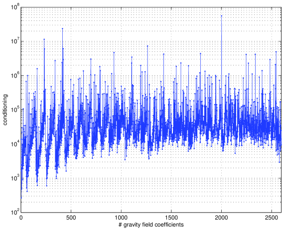
Fig. 1: Amplitude of the relative condition numbers for the gravity field coefficients.

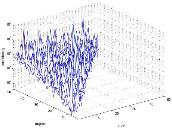
Fig. 2: Conditioning of spherical harmonic coefficients $\overline{C}_{\ell m}~{}(2\leq\ell\leq 50~{},~{}1\leq m\leq 50)$.

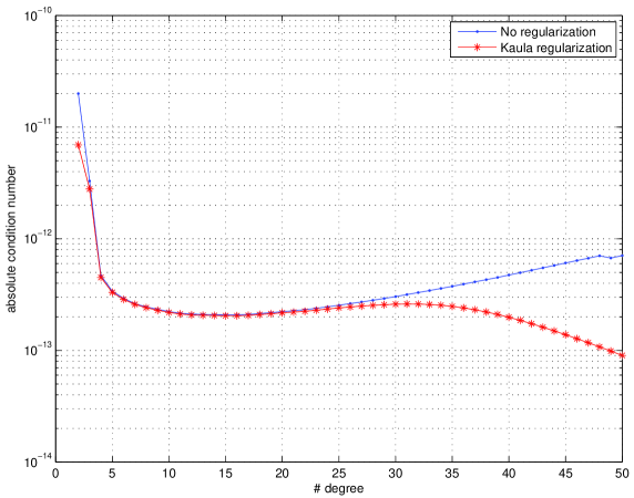
Fig. 3: Effect of regularization on zonal coefficients $\overline{C}_{{\ell}0}~{}(2\leq{\ell}\leq 50)$

6 Conclusion

To assess the accuracy of a linear least squares solution, the practitioner of numerical linear algebra uses generally quantities like condition numbers or backward errors when the statistician is more interested in covariance analysis. In this paper we proposed quantities that talk to both communities and that can assess the quality of the solution of a least squares problem or one of its component. We provided pratical ways to compute these quantities using (Sca)LAPACK and we experimented these computations on pratical examples including a real physical application in the area of space geodesy.

References

- [1] E. Anderson, Z. Bai, C. Bischof, S. Blackford, J. Demmel, J. Dongarra, J. D. Croz, A. Greenbaum, S. Hammarling, A. McKenney, and D. Sorensen, LAPACK Users’ Guide, Society for Industrial and Applied Mathematics, 3 ed., 1999.
- [2] M. Arioli, M. Baboulin, and S. Gratton, A partial condition number for linear least-squares problems, SIAM J. Matrix Anal. and Appl., 29 (2007), pp. 413–433.
- [3] M. Baboulin, Solving large dense linear least squares problems on parallel distributed computers. Application to the Earth’s gravity field computation, PhD thesis, 2006. Institut National Polytechnique de Toulouse.
- [4] G. Balmino, A. Cazenave, A. Comolet-Tirman, J. C. Husson, and M. Lefebvre, Cours de géodésie dynamique et spatiale, ENSTA, 1982.
- [5] Å. Björck, Numerical Methods for Least Squares Problems, Society Society for Industrial and Applied Mathematics, 1996.
- [6] L. S. Blackford, J. Choi, A. Cleary, E. D’Azevedo, J. Demmel, I. Dhillon, J. Dongarra, S. Hammarling, G. Henry, A. Petitet, K. Stanley, D. Walker, and R. C. Whaley, ScaLAPACK Users’ Guide, Society for Industrial and Applied Mathematics, 1997.
- [7] S. Chandrasekaran and I. C. F. Ipsen, On the sensitivity of solution components in linear systems of equations, SIAM J. Matrix Anal. and Appl., 16 (1995), pp. 93–112.
- [8] J. Demmel, Y. Hida, X. S. Li, and E. J. Riedy, Extra-precise iterative refinement for overdetermined least squares problems, Tech. Rep. EECS-2007-77, UC Berkeley, 2007. Also LAPACK Working Note 188.
- [9] R. W. Farebrother, Linear least squares computations, Marcel Dekker Inc. editions, 1988.
- [10] A. J. Geurts, A contribution to the theory of condition, Numerische Mathematik, 39 (1982), pp. 85–96.
- [11] S. Gratton, On the condition number of linear least squares problems in a weighted Frobenius norm, BIT Numerical Mathematics, 36 (1996), pp. 523–530.
- [12] T. N. A. Group, NAG Library Manual, Mark 21, NAG, 2006.
- [13] W. W. Hager, Condition estimates, SIAM J. Sci. Statist. Comput., 5 (1984), pp. 311–316.
- [14] N. J. Higham, Accuracy and Stability of Numerical Algorithms, Society Society for Industrial and Applied Mathematics, 2 ed., 2002.
- [15] N. J. Higham and G. W. Stewart, Numerical linear algebra in statistical computing, in The State of the Art in Numerical Analysis, A. Iserles and M. J. D. Powell, eds., Oxford University Press, 1987, pp. 41–57.
- [16] W. M. Kaula, Theory of satellite geodesy, Blaisdell Press, Waltham, Mass., 1966.
- [17] C. S. Kenney, A. J. Laub, and M. S. Reese, Statistical condition estimation for linear least squares, SIAM J. Matrix Anal. and Appl., 19 (1998), pp. 906–923.
- [18] J. Langou, Review of ”théorie analytique des probabilités. premier supplément. sur l’application du calcul des probabilités à la philosophie naturelle” from P. S. Laplace, tech. rep., CU Denver, 2007.
- [19] P. S. Laplace, Premier supplément. Sur l’application du calcul des probabilités à la philosophie naturelle, in Théorie Analytique des Probabilités, Mme Ve Courcier, 1820, pp. 497–530.
- [20] M. Zelen, Linear estimation and related topics, in Survey of numerical analysis, J.Todd, ed., McGraw-Hill book company, 1962, pp. 558–584.