Grain boundary diffusion in a Peierls-Nabarro potential

Abstract

We investigate the diffusion of a grain boundary in a crystalline material. We consider in particular the case of a regularly spaced low-angle grain boundary schematized as an array of dislocations that interact with each other through long-range stress fields and with the crystalline Peierls-Nabarro potential. The methodology employed to analyze the dynamics of the center of mass of the grain boundary and its spatio-temporal fluctuations is based on over-damped Langevin equations. The generality and the efficiency of this technique is proved by the agreement with molecular dynamics simulations.

1 Introduction

Understanding interface kinetics in materials is an important theoretical and practical problem, since this process influences the microstructure, such as the grain size, the texture, and the interface type. From the theoretical point of view, the study of processes that involve surface and interface properties gained significant interest in non-equilibrium statistical mechanics [1, 2]. In particular, dislocations [3, 4] and grain boundaries [5, 6] provide a concrete example of driven elastic manifolds in random media [7]. Other example of this general problem are domain walls in ferromagnets [8, 9], flux line in type II superconductors [10, 11], contact lines [12, 13] and crack fronts [14, 15]. From the point of view of applications, understanding grain boundary kinetics has a great importance for polycrystalline materials, since the resulting grain microstructure determines material properties such as strength, hardness, resistance to corrosion, conductivity etc. [16]. Hence the ambitious goal of these studies is to be able to control the microstructural properties of polycrystals.

Several approaches have been employed in the literature to study grain boundary kinetics. Ref. [17] employs molecular dynamics (MD) simulations with appropriate interatomic interactions to study the diffusion of grain boundaries at the atomic scale [17]. The method allows to quantify the mobility of grain boundaries and to compare the results with experiments [17]. While MD simulations provide a very accurate description of the dynamics, the method suffers from numerical limitations and it is difficult to reach the asymptotic regime. An alternative method is provided by the Langevin approach in which the grain boundary is assumed to evolve stochastically in an external potential [18]. The dynamics of the underlying crystalline medium enters in the problem only through the noise term (due to lattice vibrations) and the periodic potential (Peierls-Nabarro). Hence, the equations of motion of the atoms or molecules are not directly relevant. Indeed there is experimental evidence in supporting of separation of time scales in plastic flow [19] and it is thus possible to integrate out the fast degrees of freedom (atomic vibrations) and consider only the slow ones (dislocations position).

Here we study the evolution of a grain boundary (GB) in a crystalline material by the Langevin approach. The GB is treated as an array of interacting dislocations performing a thermally activated motion in a periodic (Peierls-Nabarro) potential. Similar models have been employed in the past to study the conductivity of superionic conductors [20, 21], the relaxational dynamics of rotators [22] and Josephson tunneling junctions [18]. Notice that the crucial role played by long-range stresses is often disregarded in analyzing GB deformation. On the other hand, it has been shown in Ref. [5] that a surface tension approximation for the GB stiffness is inappropriate and one has to consider explicitly non-local interactions. The present model incorporates this effect in the equations of motion.

We simulate the set of Langevin equations numerically to describe the GB kinetics and its fluctuations. The results are in good agreement with MD simulations [17] and allow to clarify the origin of the short time deviations from the diffusive behavior observed in Ref. [17]. In addition, a linearized version of the model can be treated analytically and the asymptotic results are found in good agreement with the simulations. The manuscript is organized as follows: in Sec. II we introduce the model, which is first studied in the flat GB limit in Sec. III. Sec. IV presents numerical simulations of the full flexible GB problems and Sec. V discusses the continuum theory. Sec. VI is devoted to conclusions.

2 The model

To study the GB dynamics we consider a phenomenological mesoscopic approach. We consider in particular the case of a regularly spaced low-angle grain boundary schematized as an array of straight dislocations that interact with each other through long-range stress fields and with the crystalline Peierls-Nabarro (PN) potential. The GB is composed by $N$ dislocations where configurations are repeated ad infinitum because of periodic boundary conditions along the $y$ direction. Each dislocation has Burger vector of modulus $b$ parallel to the $x$ axis and the distance between two adjacent dislocations along the $y$ direction is fixed to be $a$. Each straight dislocation interacts with the lattice and with others dislocations through long-range stress fields. The effect of the lattice over each n-th dislocation can be decomposed as the sum of three contributions:

• $F_{PN}(x_{n})=-\mathcal{A}\frac{\mbox{\normalsize{$\mu b$}}}{\mbox{\normalsize{$2\pi r_{0}$}}}\sin(\frac{\mbox{\normalsize{$2\pi x_{n}$}}}{\mbox{\normalsize{$b$}}})$, the PN force where $\mathcal{A}$ is the area of the GB, $\mu$ is the shear modulus and $r_{0}$ the inter-atomic distance;

• -$\gamma\dot{x}_{n}(t)$, the average effect of the lattice fluctuations where $\gamma$ is the viscosity coefficient;

• $\gamma\eta_{n}(t)$, the impulsive effect of the lattice fluctuations assumed to be Gaussian for the central limit theorem and uncorrelated in space and time: $\langle\eta_{n}(t)\rangle=0$, $\langle\eta_{n}(t)\eta_{m}(t^{\prime})\rangle=D\delta_{nm}\delta(t-t^{\prime})$ where $D$ is the diffusion coefficient [18].

The long-range stress field exercised by all the other dislocations over the n-th, the Peach-Koehler force $F_{PK}^{n,N}({\bf x},{\bf y})$, is computed considering the image dislocations method to comply with periodic boundary conditions along the $y$ direction. Making use of calculations in [23, 24] one can find the following expression

$$\begin{array}[]{l}F_{PK}^{n,N}({\bf x},{\bf y})=-\frac{\mbox{\normalsize{$\mu b^{2}\pi$}}}{\mbox{\normalsize{$N^{2}a^{2}(1-\nu)$}}}\sum_{m=1}^{N}(x_{n}-x_{m})\cdot\\ \\ \cdot\frac{\mbox{\normalsize{$\{\cosh[2\pi(x_{n}-x_{m})/Na]\cos[2\pi(y_{n}-y_{m})/Na]-1\}$}}}{\mbox{\normalsize{$\{\cosh[2\pi(x_{n}-x_{m})/Na]-\cos[2\pi(y_{n}-y_{m})/Na]\}^{2}$}}},\end{array}$$ (1)

where $\nu$ is the Poisson’s ratio, $y_{n}=n\cdot a$ and $y_{m}=m\cdot a$. Finally the over-damped Langevin equation [18] for the GB reads

$$\gamma\dot{x}_{n}(t)=F_{PN}(x_{n})+F_{PK}^{n,N}({\bf x},{\bf y})+\gamma\eta_{n}(t),$$ (2)

for $n=1,...,N$, or rather

$$\begin{array}[]{l}\dot{x}_{n}(t)=-\mathcal{A}\frac{\mbox{\normalsize{$\mu b$}}}{\mbox{\normalsize{$2\pi r_{0}\gamma$}}}\sin(\frac{\mbox{\normalsize{$2\pi x_{n}$}}}{\mbox{\normalsize{$b$}}})-\frac{\mbox{\normalsize{$\mu b^{2}\pi$}}}{\mbox{\normalsize{$N^{2}a^{2}(1-\nu)\gamma$}}}\sum_{m=1}^{N}(x_{n}-x_{m})\cdot\\ \\ \cdot\frac{\mbox{\normalsize{$\{\cosh[2\pi(x_{n}-x_{m})/Na]\cos[2\pi(y_{n}-y_{m})/Na]-1\}$}}}{\mbox{\normalsize{$\{\cosh[2\pi(x_{n}-x_{m})/Na]-\cos[2\pi(y_{n}-y_{m})/Na]\}^{2}$}}}+\eta_{n}(t).\end{array}$$ (3)

To indicate the amplitude of the $F_{PN}$ and $F_{PK}$ forces we introduce respectively the parameters $A_{PN}=\mathcal{A}\mu b/2\pi r_{0}\gamma$ and $A_{PK}=\mu b^{2}\pi/a^{2}(1-\nu)\gamma$.

The key quantities that we consider in order to characterize the dynamics of the GB are:

• the mean-square displacement of the center of mass, $\Delta x_{cm}(t)=\langle x_{cm}^{2}(t)\rangle-\langle x_{cm}(t)\rangle^{2}=\langle\overline{x_{n}(t)}^{2}\rangle-\langle\overline{x_{n}(t)}\rangle^{2}$ where $x_{cm}(t)=\overline{x_{n}}=1/N\sum_{n=1}^{N}x_{n}(t)$;

• the mean-square width $W^{2}(t)=\overline{\langle x_{n}^{2}\rangle}-\langle(\overline{x_{n}})^{2}\rangle$.

In the following, we first analyze the case of a flat GB for which a comparison with MD simulations approach [17] is made. Next we consider the full flexible description of the GB. Finally, we discuss a linearized version of the model that can be treated analytically.

3 Flat grain boundary

For many applications a good approximation is to consider a flat GB with a single degree of freedom, for which $F_{PK}^{n,L}({\bf x},{\bf y})=0$ and $x_{n}(t)=x_{cm}(t)$ for $n=1,...,N$. In other words, the flat GB is described by the following equation

$$\dot{x}_{cm}(t)=-\mathcal{A}\frac{\mu b}{2\pi r_{0}\gamma}\sin(\frac{2\pi x_{cm}}{b})+\eta(t),$$ (4)

where the correlation properties of the thermal fluctuations are: $\langle\eta(t)\rangle=0$ and $\langle\eta(t)\eta(t^{\prime})\rangle=D\delta(t-t^{\prime})$. This type of equation, also known as the Kramers equation with periodic potential, has been extensively studied in the literature [18]. In particular, the mean-square displacement is known to display a combination of oscillatory and diffusive behavior [18, 25]. Different dynamical regimes are found as the potential strength or the friction varies [25]. In fact, we show next that this simple model allows to understand the short-time deviations from diffusive behavior observed in MD simulations [17].

Integrating Eq. 4 with the initial condition $x_{cm}(0)=0$ by means of computer simulations (fitting $D$ and $\gamma$ with the condition $D\gamma=D_{R}/\mathcal{M}$ [18] where $\mathcal{M}$ is the mobility and $D_{R}$ is the renormalized diffusion coefficient considered in [17]), we have compared the mean-square displacement $\Delta x_{cm}(t)$ to the one obtained from MD simulation in Ref. [17]. In Fig. 1 this comparison is displayed together with the mean-square displacement of the renormalized free Brownian motion (described by the equation: $\dot{x}=\eta(t)$ with $\langle\eta(t)\rangle=0$ and $\langle\eta(t)\eta(t^{\prime})\rangle=D_{R}\delta(t-t^{\prime})$). The agreement between the two simulations is extremely good. For higher times ($t>80ps$), the mean-square displacement tends to the renormalized Brownian motion. Hence taking explicitly into account the sinusoidal Peierls-Nabarro force in the Langevin equation allows to describe the mean-square displacement for early times of the dynamics.

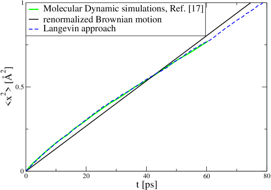
Figure 1: Mean-square displacement $\Delta x_{cm}(t)$ of the flat grain boundary comparison between molecular dynamic simulation [17] (green line) and Langevin approach simulation (dashed blue line). Both type of simulations predicts a linear dependence in time of $\Delta x_{cm}(t)$ for long times represented in the figure by the renormalized free Brownian motion (straight black line).

One can deduce in a simplified intuitive way the temporal evolution of the mean-square displacement starting by the transition probability density $P$ for small times (small $\tau$) [18]

$$P(x,t+\tau|x^{\prime},t)=\frac{1}{2\sqrt{\pi D\tau}}\ \ \mbox{\Large{$e$}}^{\mbox{\large{$-\frac{[x-x^{\prime}-F_{PN}(x)\tau]^{2}}{4D\tau}$}}}.$$ (5)

Next we consider the transition probability $P_{01}(x_{0}+\Delta x_{1},t_{0}+\tau|x_{0},t_{0})$ to run from the point $x_{0}$ at time $t_{0}$ to the point $x_{1}=x_{0}+\Delta x_{1}$ at time $t_{1}=t_{0}+\tau$ and $P_{12}(x_{0}+\Delta x_{1}+\Delta x_{2},t_{0}+2\tau|x_{0}+\Delta x_{1},t_{0}+\tau)$ to run from $x_{1}$ at $t_{1}$ to $x_{2}=x_{1}+\Delta x_{2}$ at $t_{2}=t_{1}+\tau$

$$\left\{\begin{array}[]{rll}P_{01}&=&\mbox{\Large{$\frac{1}{2\sqrt{\pi D\tau}}$}}\ \ \mbox{\Large{$e$}}^{\mbox{\large{$-\frac{[\Delta x_{1}-F_{PN}(x_{0})\tau]^{2}}{4D\tau}$}}}\\ &&\\ P_{12}&=&\mbox{\Large{$\frac{1}{2\sqrt{\pi D\tau}}$}}\ \ \mbox{\Large{$e$}}^{\mbox{\large{$-\frac{[\Delta x_{2}-F_{PN}(x_{0}+\Delta x_{1})\tau]^{2}}{4D\tau}$}}}.\\ \end{array}\right.$$ (6)

For a free Brownian motion ($F_{PN}(x)=0$) the condition $P_{01}=P_{12}$ implies $\Delta x_{1}=\Delta x_{2}$ and stochastic displacements are space independent. If we impose this condition in presence of a periodic force $F_{PN}(x)=-dU_{PN}(x)/dx$, we obtain

$$\begin{array}[]{l}P_{01}=P_{12}\ \ \Rightarrow\ \ \Delta x_{1}-F_{PN}(x_{0})\tau=\Delta x_{2}-F_{PN}(x_{0}+\Delta x_{1})\tau\ \ \Rightarrow\\ \\ \Rightarrow\ \ \Delta x_{2}=\Delta x_{1}\left[1+\left.\mbox{\large{$\frac{dF_{PN}(x)}{dx}$}}\right|_{x_{0}}\tau\right],\end{array}$$ (7)

and then

$$\Delta x_{2}\gtrless\Delta x_{1}\ \ \ \ \mbox{if}\ \ \ \ \left.\frac{dF_{PN}}{dx}\right|_{x_{0}}\gtrless 0\ \ \ \ \mbox{or rather}\ \ \ \ \left.\frac{d^{2}U_{PN}}{dx^{2}}\right|_{x_{0}}\lessgtr 0.$$ (8)

This result implies that, with the initial condition $x_{cm}(0)=0$, if the potential $U_{PN}(x)$ is convex (concave) the mean-square displacement curve is concave (convex). In the case of the PN potential, we find indeed that the mean-square displacement curve should display upper and lower deviations from the straight line, corresponding to a renormalized free Brownian motion, depending in $d^{2}U_{PN}(x)/dx^{2}$. These deviations decrease with time so that for large times the curve should approach a straight line [18].

4 Flexible grain boundary

A more general description of the GB considers its internal deformation and the dynamics is described by Eq. 3. The dynamical behavior of the GB depends on the amplitude of the three terms in the right-hand side of Eq. 3.

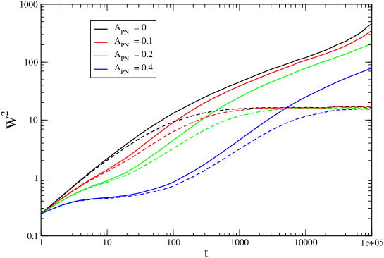
Figure 2: Mean-square width of the grain boundary, $W^{2}(t)$, in the case of $N=32$ for the two typical situation in which (continuum line) the GB exfoliate ($W^{2}(t)$ increase with time) because the noise is high enough respect to $A_{PK}$ and to $A_{PN}$, (dashed line) the GB reach a stationary state ($W^{2}(t)$ saturates after a certain time) because the noise is small enough respect to $A_{PK}$ or to $A_{PN}$.

The parameters that characterize the behavior of the GB are $a$, $b$, $A_{PK}$, $A_{PN}$ and $D$. Varying the values of these parameters, in the long-time limit the GB can either exfoliate (when the noise, $D$, is high enough with respect to $A_{PK}$ and to $A_{PN}$) or reach a stationary state (when the noise, $D$, is small when compared to $A_{PK}$ or to $A_{PN}$). The asymptotic behavior can be read off from the width $W^{2}(t)$ that keeps on increasing when the GB exfoliates and saturates when the GB remains stable. In Fig. 2 the comparison between these two typical situations is displayed in the case of $N=32$, $a=b=3\pi$, $A_{PN}=0,0.1,0.2,0.4$, $D=0.25$ and $A_{PK}=0.14$ for the case in which the GB remains stable, while $A_{PK}=0.0896$ for the case in which the GB exfoliates.

In what follows, we analyze the dynamical behavior of the stable GB for $a=b=3\pi$, $A_{PN}=0,0.4$, $A_{PK}=0.14$ and $D=0.25$. In Fig. 3 the average position of the GB center of mass $\Delta x_{cm}(t)$ is displayed with and without the PN force in Log-Log scale for $N=32,64,128,256,512$.

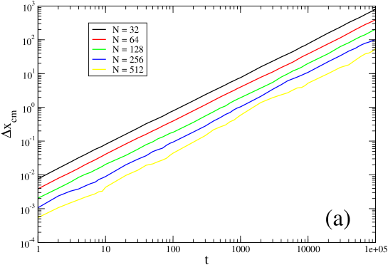
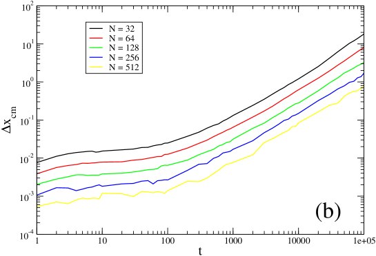
Figure 3: Mean-square displacement of the center of mass of the grain boundary, $\Delta x_{cm}(t)$ , for Langevin approach simulation without the PN force (a) and with the PN force (b). $\Delta x_{cm}(t)$ for $N=32,64,128,256,512$ is displayed in Log-Log scale.

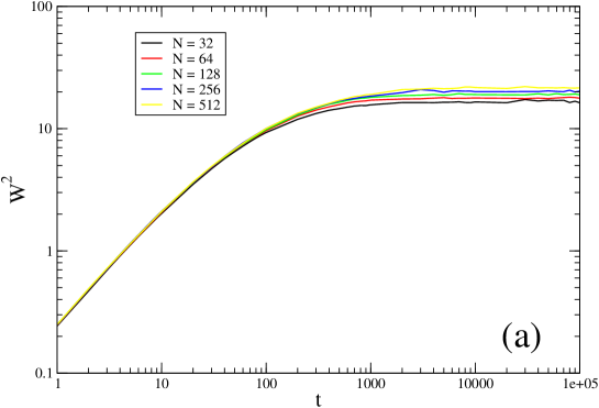
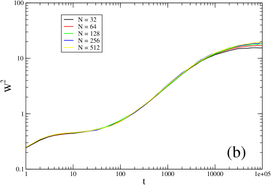
Figure 4: Mean-square width of the grain boundary, $W^{2}(t)$, for Langevin approach simulation without the PN force (a) and with the PN force (b). $W^{2}(t)$ for $N=32,64,128,256,512$ is displayed in Log-Log scale.

For long times in both cases we have a linear behavior $\Delta x_{cm}(t)\sim t$, but for short times, in the presence of the PN force, there is a clear deviation from linearity. This result confirms the conclusion made in the previous section, that the PN force is the cause for the deviation from linearity of $\Delta x_{cm}(t)$ for short times observed in Ref. [17]. Next we characterize the morphology of the GB through the width $W^{2}(t)$. In Fig. 4 $W^{2}(t)$ for $N=32,64,128,256,512$ is displayed with and without the PN force in Log-Log scale. In the absence of the PN force (Fig. 4a) the time dependence of $W^{2}(t)$ is qualitatively similar to the same case but with linearized PK force discussed in the next section, while in the presence of the PN force, for $A_{PN}=0.4$ (Fig. 4b), $W^{2}(t)$ exhibit a plateau for intermediate times.

5 Continuum Theory

It is possible to develop an analytic expression in the continuum limit ($a\rightarrow 0$, $N\rightarrow\infty$ and $L=Na=const.$) for short or long times for $W^{2}(t)$ in absence of the PN force linearizing the PK force. The equation of motion for $F_{PN}=0$ and $F_{PK}$ linearized is

$$\dot{x}_{n}(t)=-\frac{\mu b^{2}}{2\pi(1-\nu)\gamma}\sum_{m=1}^{N}\frac{x_{n}-x_{m}}{(y_{n}-y_{m})^{2}}+\eta_{n}(t).$$ (9)

To obtain the short time behavior is sufficient to rewrite Eq. 9 as a generalized Ornstein-Uhlenbeck process [18]

$$\dot{x}_{n}(t)=\sum_{m=1}^{N}g_{nm}x_{m}+\eta_{n}(t).$$ (10)

The general solution of Eq. 10 is

$$x_{n}(t)=\int_{0}^{\infty}\sum_{m=1}^{N}G_{nm}(t^{\prime})\eta_{m}(t-t^{\prime})dt^{\prime},$$ (11)

with $\{G_{nm}(t)\}=\hat{G}(t)=e^{\hat{g}t}=\mathbbm{1}+\hat{g}t+\hat{g}^{2}t^{2}/2+...$ (where $\mathbbm{1}=\{\delta_{ij}\}$). From the definition of $W^{2}(t)$, results

$$W^{2}(t)=\frac{D}{N}\sum_{n,m=1}^{N}\int_{0}^{t}G_{nm}^{2}(t^{\prime})dt^{\prime}-\frac{D}{N^{2}}\sum_{n,m,l=1}^{N}\int_{0}^{t}G_{nm}(t^{\prime})G_{lm}(t^{\prime})dt^{\prime}.$$ (12)

Replacing the Taylor expansion of the $\hat{G}$ matrix in Eq. 12 one obtains for short times ($t\ll 1/\|\hat{g}\|$) that $W^{2}(t)=(1-1/N)Dt+o(t)$ and in the continuum limit $W^{2}(t)=Dt+o(t)$. To obtain the long times behavior of $W^{2}(t)$, we rewrite Eq. 9 in Fourier space [5, 26]. Employing the decomposition $x_{m}=1/L\sum_{k}exp(-ikam)x_{k}$, we obtain

$$\dot{x}_{k}=-\frac{\mu b^{2}}{2\pi(1-\nu)\gamma a^{2}L}\sum_{m=-\infty}^{\infty}e^{ikam}\sum_{n=-\infty}^{\infty}\frac{\sum_{k^{\prime}}(e^{-ik^{\prime}am}-e^{-ik^{\prime}an})x_{k^{\prime}}}{(m-n)^{2}}+\eta_{k}.$$ (13)

The first term in the right-hand side of Eq. 13 can be rewritten as

$$-\frac{\mu b^{2}}{2\pi(1-\nu)\gamma a^{2}L}\sum_{k^{\prime}}x_{k^{\prime}}\sum_{m=-\infty}^{\infty}e^{i(k-k^{\prime})am}(\sum_{d=-\infty}^{\infty}\frac{1-e^{ik^{\prime}ad}}{d^{2}}),$$ (14)

where $d=m-n$. Using the following results

$$\sum_{d=1}^{\infty}\frac{1}{d^{2}}=\frac{\pi^{2}}{6},\ \ \ \ \sum_{d=1}^{\infty}\frac{cos(cd)}{d^{2}}=\frac{\pi^{2}}{6}-\frac{\pi|c|}{2}+\frac{c^{2}}{4},$$ (15)

we obtain

$$\sum_{d=-\infty}^{\infty}\frac{1-e^{ik^{\prime}ad}}{d^{2}}=2\sum_{d=1}^{\infty}\frac{1-\cos(k^{\prime}ad)}{d^{2}}=\pi|k^{\prime}|a-\frac{k^{\prime 2}a^{2}}{2},$$ (16)

so that Eq. 13 becomes

$$\dot{x}_{k}=-\frac{\mu b^{2}}{2\pi(1-\nu)\gamma a^{2}}(\pi|k|-\frac{k^{2}a}{2})x_{k}+\eta_{k}.$$ (17)

In the long time limit (large $x$, small $k$) the $k^{2}$ term can be neglected. Finally in the continuum limit we replace $y_{n}$, $y_{m}$ by the continuum variables $y$, $y^{\prime}$ and $\langle\eta(y,t)\eta(y^{\prime},t^{\prime})\rangle=aD\delta(y-y^{\prime})\delta(t-t^{\prime})$.

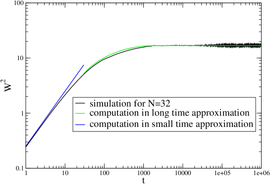
Figure 5: Comparison between the mean-square width $W^{2}(t)$ for linearized $F_{PK}$ and $F_{PN}=0$ in the case of $N=32$ computed by numerical simulation and the continuum theoretical prediction in the short and long times limit. The black line represents the simulated data, the green line the long times theoretical prediction with fitted parameters and the blue line the short times theoretical prediction.

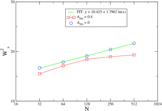
Figure 6: Size dependence for the saturation value of the mean-square width $W^{2}_{s}$ in Log scale for the abscissa (x-axis). As can be seen in figure, in the case in which the PN force is absent ($A_{PN}=0$) the relation is logarithmic ($W^{2}_{s}\sim\log N$), while in presence of the PN force ($A_{PN}\neq 0$) a slight deviation from the logarithmic dependence is observed.

Thus Eq. 13 becomes

$$\dot{x}_{k}=-\alpha|k|x_{k}+\eta_{k},$$ (18)

where $\alpha=\mu b^{2}/[2(1-\nu)\gamma a^{2}]$. Eq. 18 can be solved exactly and $W^{2}(t)$ is given by [2, 27]

$$W^{2}(t)=\frac{aD}{2\pi\alpha}[\ln(\frac{L}{a})+\ln(1-e^{-4\pi\alpha t/L})].$$ (19)

To reproduce the continuum limit by simulations of Eq. 9 we would need a very large GB, with $N\gg 512$. Thus a comparison between Eq. 19 and the simulations for small $N$ is possible only by introducing some effective parameters in Eq. 19. In Fig. 5 $W^{2}(t)$ computed by the simulations with $N=32$ (for which the better statistic is available) is compared with the fitted theoretical prediction for short and long times. Eq. 19 also predicts that the saturated value of width ($W^{2}_{s}$) exhibits a logarithmic dependence on the GB length $L=N/a$: $W^{2}_{s}\sim\log N$. In the case in which $F_{PK}$ is not linearized this result is also confirmed by numerical simulations, showing that $W_{s}^{2}$ increases logarithmically with $N$ when $F_{PN}=0$ (see Fig. 6). In presence of a periodic potential ($F_{PN}>0$), however, we observe a deviation from the logarithmic growth at large $N$. This suggests that the Peierls-Nabarro potential may set a limit to the GB roughness.

6 Summary and Discussion

We have investigated the diffusion of a regularly spaced low-angle grain boundary in a crystalline material. A typical computational method to describe the dynamics of the grain boundary is to perform deterministic molecular dynamics simulations with appropriate interatomic interactions [17]. Here we have employed the over-damped Langevin approach to obtain a long time description of the dynamics, but in particular to perform a comparison with molecular dynamics simulations for a specific material [17]. The first results is the interpretation of the early times behavior of the mean-square displacement $\Delta x_{cm}(t)$. The deviation for early times of $\Delta x_{cm}(t)$ by the case of the renormalized Brownian motion, that holds for long times, can be interpreted as the effect on the dislocations of the periodicity of the lattice giving rise to the Peierls-Nabarro potential. Secondly the description of the dynamic ($\Delta x_{cm}(t)$) and the morphology ($W^{2}(t)$) of the grain boundary by means of over-damped Langevin equations is in qualitatively good agreement with its behavior in real materials, so this approach can be considered an useful tool for these studies.

References

References

- [1] Barabàsi A L and Stanley H E 1995 Fractal Concepts in Surface Growth (Cambridge University Press)
- [2] Krug J 1997 Adv. Phys. 46 139
- [3] Zaiser M 2006 Adv. Phys. 54 185
- [4] Zapperi S and Zaiser M 2001 Mat. Sci. and Eng. A 348 309
- [5] Moretti P, Miguel MC, Zaiser M, and Zapperi S 2004 Phys. Rev. B 69 214103.
- [6] Moretti P, Miguel MC and Zapperi S 2005 Phys. Rev. B 72 014505.
- [7] Kardar M 1998 Phys. Rep. 301 85
- [8] Lemerle S, Ferré J, Chappert C, Mathet V, Giamarchi T and Le Doussal P 1998 Phys. Rev. Lett. 80 849
- [9] Zapperi S, Cizeau P, Durin G and Stanley H E 1998 Phys. Rev. B 58 6353
- [10] Bhattacharya S and Higgins M J 1993 Phys. Rev. Lett. 70 2617
- [11] Surdeanu R, Wijngarden R J, Visser E, Huijbregtse J M, Rector J H, Dam B and Griessen R 1999 Phys. Rev. Lett. 83 2054
- [12] Schäffer E and Wong P z 2000 Phys. Rev. E 61 5257
- [13] Rolley E, Guthmann C, Gombrowicz R and Repain V 1998 Phys. Rev. Lett. 80 2865
- [14] Bouchaud E 1997 J. Phys. C 9 4319
- [15] Schmittbuhl J and Måløy K 1997 Phys. Rev. Lett. 78 3888
- [16] Sutton A P and Balluffi R W 1995 Interfaces in Crystalline Materials (Monographs on the Physics and Chemistry of Materials, Clarendon Press)
- [17] Trautt Z T, Upmanyu M and Karma A 2006 Science 314 632
- [18] Risken H 1984 The Fokker-Plank Equation (Springer Verlag)
- [19] Ananthakrishna G 2007 Phys. Rep. 440 113-259
- [20] Fulde P, Pietronero L, Schneider W R and Strässler S 1975 Phys. Rev. Lett. 35 1776
- [21] Dieterich W, Fulde P and Peschel I 1980 Adv. Phys. 29 527
- [22] Marchesoni F and Vij J K 1985 Z. Phys. B 58 187
- [23] Hirth J P and Lothe J 1982 Theory of Dislocations (Wiley & Sons)
- [24] Friedel J 1964 Dislocations (Pergamon Press)
- [25] Ferrando R, Spadacini R, Tommei G E and Caratti G 1992 Physica A 195 506-532
- [26] Chui ST 1983 Phys. Rev. B 28 178
- [27] Krug J and Meakin P 1991 Phys. Rev. Lett. 66 703