The Student ensemble of correlation matrices: eigenvalue spectrum and Kullback-Leibler entropy

Abstract

We study a new ensemble of random correlation matrices related to multivariate Student (or more generally elliptic) random variables. We establish the exact density of states of empirical correlation matrices that generalizes the Marčenko-Pastur result. The comparison between the theoretical density of states in the Student case and empirical financial data is surprisingly good, even if we are still able to detect systematic deviations. Finally, we compute explicitely the Kullback-Leibler entropies of empirical Student matrices, which are found to be independent of the true correlation matrix, as in the Gaussian case. We provide numerically exact values for these Kullback-Leibler entropies.

I Introduction

Estimating and analyzing the correlation matrix of $N$ different variables from a data set is very recurrent problem in statistical analysis. Typically, one observes the value of the $N$ different variables over a time period of size $T$. The total number of data point is $NT$ whereas the number of elements of the correlation matrix is $N(N-1)/2$. In many applications, both $T$ and $N$ are large but $Q=T/N$ is of order unity. For example, in financial applications the values of $T$ and $N$ go from few hundreds to a few thousands. In these cases, the correlation (or covariance) matrix is in fact rather poorly determined. This means, in particular, substantial noise in the determination of the eigenvalues and eigenvectors. For instance, focus on the case where all random variables are in fact independent, such that the true correlation matrix $C_{ij}$ is the identity matrix. The empirical determination of ${\bf C}$, which we call ${\bf E}$, is obtained from the zero mean, unit variance Gaussian variables $r_{i}^{t}$ using the Pearson estimator:

$$E_{ij}=\frac{1}{T}\sum_{t}^{T}r^{t}_{i}r^{t}_{j}$$ (1)

The eigenvalue spectrum $\rho(\lambda)$ of ${\bf E}$ only approaches a $\delta$-function at $\lambda=1$ when $Q\to\infty$. When $Q$ is finite, however, $\rho(\lambda)$ is non-trivial. Under mild hypothesis about the distribution of the $r_{t}^{i}$s (essentially that the variance is finite), the spectrum approaches, in the large $N,T$ limit, the Marčenko-Pastur distribution marcenkopastur :

$$\rho(\lambda)=\frac{\sqrt{4\lambda q-(\lambda-1+q)^{2}}}{2\pi\lambda q}\qquad\lambda\in[(1-\sqrt{q})^{2},(1+\sqrt{q})^{2}]\quad(q=1/Q<1).$$ (2)

For finite $N$, the edges of the spectrum are smoothed. The statistics of exceptionally large eigenvalues is described by the Tracy-Widom distribution GBA , or by a Fréchet distribution when the $r_{t}$ have power-law tails decaying sufficiently slowly BBP . The probability of large fluctuations of the maximum eigenvalue (for Gaussian $r_{t}$) has been derived in VMB .

In this work we focus on a more general ensemble that often provides a faithful representation of empirical data. We will consider that the random variables $r_{i}^{t}$ can be written as a product of two terms: $r_{i}^{t}=\sigma^{t}\eta_{i}^{t}$ where $\eta_{i}^{t}$ and $\sigma^{t}$ are independent random variables. The $\eta_{i}^{t}$ are characterized by a true correlation matrix $C_{ij}=\langle\eta_{i}\eta_{j}\rangle$ and $\sigma_{i}^{t}$ are such that $\langle\sigma^{2}\rangle=1$. Furthermore, $\eta_{i}^{t}$ are drawn independently from the same distribution at each time $t$. A particular case on which we shall focus extensively corresponds to Gaussian distributed $\eta_{i}$ and

$$P(\sigma)=\frac{2}{\Gamma(\frac{\mu}{2})}\exp\left[-\frac{\sigma_{0}^{2}}{\sigma^{2}}\right]\frac{\sigma_{0}^{\mu}}{\sigma^{1+\mu}},$$ (3)

where $\sigma_{0}^{2}=2\mu/(\mu-2)$ in such a way that $\langle\sigma^{2}\rangle=1$ ($\Gamma(x)$ is the Gamma function). This case corresponds to a multivariate Student distribution for the original variables $r_{i}^{t}$. This defines the Student Ensemble we will consider more specifically below, although many of our results extend to arbitrary choice of $P(\sigma)$ and $P(\{\eta_{i}^{t}\})$, defining a large class of elliptic distributions. We will also focus on applications of our results to finance where the correct determination of the true correlation matrix between stocks play a very important role.

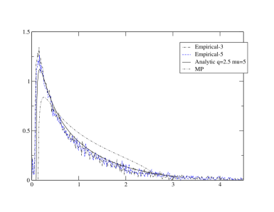
Figure 4: Comparison between the analytical results, Student (for $\mu=5$) and Gaussian Wishart, and the empirical data.

The application of Random Matrix Theory to financial correlation matrices was first suggested in prl ; Plerou ; dublin ; Cracow . In this context $r_{i}^{t}$ are daily (or higher frequency) returns of $N$ different stocks over a time period of size $T$. As discussed above, even in the absence of any correlation between stocks, we expect the eigenvalues of an empirical correlation matrix, determined over a finite time interval, to be non trivial. As a consequence, distinguishing between noise and genuine information in the empirical density of states is a subtle matter. For example, the diagonalisation of the correlation matrix of, say, 450 stocks computed over a bit more than 4 years (1125 trading days) reveals one very large eigenvalue corresponding to a roughly uniform eigenvector, corresponding to the “market mode”, and a handful of other large eigenvalues that can be seen to correspond to large sectors of economic activity. Smaller eigenvalues, however, form a blob around $\lambda=1$. Is this blob well described by the Marčenko-Pastur distribution? In order to answer this question one has to rescale the small (supposedly “pure noise”) empirical eigenvalues in order to have ${\overline{\lambda}}=1$ and compare to a Marčenko-Pastur distribution (for which one has by definition ${\overline{\lambda}}=1$). Different results are obtained depending on the number of largest eigenvalues that are considered meaningful. They are shown in Figs. 3 and 4 below. The agreement between empirical data and the Marčenko-Pastur distribution is seen to be acceptable, although some systematic deviations are observed prl ; Cracow . Should these deviations then be interpreted as the presence of true economic information hidden in the noise band, or are we missing an important effect? The phenomenology of financial markets suggests that a more faithful model consists in assuming that all individual stock returns are impacted by the same, time dependent scale factor $\sigma_{t}$ that represents the “market volatility”: $r^{t}_{i}=\sigma_{t}\eta^{t}_{i}$, where $\eta_{t}^{i}$ are zero mean, unit variance Gaussian variables, and $\sigma_{t}$ is a random variable. From empirical studies, we know that the $\sigma_{t}$’s have long range temporal correlations but for the purpose of the present study we only have to specify the marginal distribution $P(\sigma)$. One possible choice that matches quite well the data is to choose Eq. (3) with $\mu\simeq 3-5$. This corresponds to a multivariate Student distribution for the returns, discussed for example in book ; Sornette . This is the model we will consider more specifically below. Another possible choice, inspired by the multifractal random walk model MRW , is a log-normal distribution for $P(\sigma)$.

II Wishart-Student matrices

II.1 Density of states of Pearson and Maximum Likelihood Estimators

The first question we address is the generalisation of the Marčenko-Pastur spectrum for multivariate Student variables, when the Pearson estimate Eq. (1) is used to determine the empirical correlation matrix. The computation of the density of states (DOS) can be straightforwardly performed using free random matrices techniques Verdu . The trick is to use the so called Blue function which is the inverse of the resolvent $G$: $B(G(z))=z$. The quantity $B(x)-1/x$ is called the R-transform of $G$ and under certain hypotheses, obeyed by any elliptic Wishart ensemble such that $C_{ij}=\langle\eta_{i}\eta_{j}\rangle=\delta_{ij}$, is known to be additive Verdu .

Since any elementary matrix $\sigma_{t}^{2}\eta_{i}^{t}\eta_{j}^{t}$ is a projector, its resolvent is simply:

$$G_{t}(z)=\frac{1}{N}\left(\frac{1}{z-\frac{\overline{\mu}}{Qs_{t}}}+\frac{N-1}{z}\right)$$ (4)

where $Q=T/N$ and $\sigma_{t}^{2}\equiv\overline{\mu}/s_{t}$ (henceforth, $\overline{\mu}=\mu/2-1$), such that $P(s)=s^{\mu/2-1}e^{-s}/\Gamma(\mu/2)$ in the Student case. We have used that in the large $N$ limit $\sum_{i}(\eta_{i}^{t})^{2}/N=1$. Inverting the resolvent at leading order we find:

$$B_{t}(x)=\frac{1}{x}+\frac{\frac{\overline{\mu}}{Qs_{t}}}{N(1-\frac{x\overline{\mu}}{Qs_{t}})}$$ (5)

Using the additive properties of the R-transform we finally find the Blue function for $\mathbf{E}$:

$$B(x)=\frac{1}{x}+\frac{1}{T}\sum_{t}\frac{\frac{\overline{\mu}}{s_{t}}}{(1-\frac{x\overline{\mu}}{Qs_{t}})}=\frac{1}{x}+\int dsP(s)\frac{\frac{\overline{\mu}}{s}}{(1-\frac{x\overline{\mu}}{Qs})}$$ (6)

where the second identity is due to the large $T,N$ limit at fixed $Q$.

The relation between the resolvent and the density of states is $G(\lambda-i\epsilon)=G_{R}(\lambda)+i\pi\rho(\lambda)$, where $G_{R}$ is the real part of the resolvent. Inverting this relation we find two coupled equations on $G_{R},\rho$:

$$\lambda = \frac{G_{R}}{G_{R}^{2}+\pi^{2}\rho^{2}}+\int dsP(s)\frac{\overline{\mu}(s-\overline{\mu}G_{R}/Q)}{(s-\overline{\mu}G_{R}/Q)^{2}+\overline{\mu}^{2}\pi^{2}\rho^{2}/Q^{2}}$$ (7)

$$0 = \rho\left(-\frac{1}{G_{R}^{2}+\pi^{2}\rho^{2}}+\int dsP(s)\frac{\overline{\mu}^{2}/Q}{(s-\overline{\mu}G_{R}/Q)^{2}+\overline{\mu}^{2}\pi^{2}\rho^{2}/Q^{2}}\right)$$ (8)

Note that these equations are actually valid for any $P(\sigma)$ (when tails are not too heavy). The last equation of course always admits the $\rho=0$ solution. At very small $\lambda$, the solution of these equations is indeed $\rho=0$. The corresponding $G_{R}$ solves the equation

$$\lambda=\frac{1}{G_{R}}+\int dsP(s)\frac{\overline{\mu}}{s-\overline{\mu}G_{R}/Q}$$ (9)

The RHS is well defined only for negative $G_{R}$, it goes to zero for very large and negative $G_{R}$, it goes to minus infinity at $G_{R}=0^{-}$ and it has a maximum somewhere in between. The maximum of the RHS corresponds to the largest value of $\lambda$ for which there is a real solution, i.e. to the left edge of the DOS. It can be determined obtaining the value of $G_{R}$ where the RHS of the previous equation has a maximum:

$$1=\int dsP(s)\frac{\overline{\mu}^{2}G_{R}^{2}/Q}{(s-\overline{\mu}G_{R}/Q)^{2}},$$ (10)

and plugging this value into (9). When $P(s)$ extends to $s=0$, as is the case for Student variables, there is no real solution for larger values of $\lambda$. This implies that the DOS has no right edge in that case. In order to determine the DOS right tails we focus on the large $\lambda$ limit of eqs (7,8). It is easy to check that Eq. (7) is solved in the large $\lambda$ limit by $G_{R}\approx 1/\lambda$ if $\rho/G_{R}$ goes to zero. We will check that this is indeed the case after having determined $\rho(\lambda)$. In order to do so, we analyze Eq. (8) assuming $\rho/G_{R}\rightarrow 0$. In this case the integral can be computed exactly and one gets (for large $\lambda$):

$$\rho(\lambda)\simeq\frac{{\overline{\mu}}^{\mu/2}}{\Gamma(\mu/2)Q^{\mu/2-1}}\frac{1}{\lambda^{1+\mu/2}}.$$ (11)

This result abides our initial assumption $\rho/G_{R}=\rho\lambda\rightarrow 0$ when $\lambda\to\infty$. It can be interpreted in terms of rare events. Indeed the distribution of $\sigma$ has exactly the same power law tail. A very large $\sigma^{*}$ on a given day, $t$, leads to an quasi-eigenvalue $\lambda\simeq\sigma^{*2}/Q$ plus subleading contribution. As a consequence, writing (for $s<<1,\lambda>>1$) $TP(s)ds=N\rho(\lambda)d\lambda$ allows one recover precisely the left tail of the DOS. As expected, provided $\mu>2$, the power-tail disappears in the limit $Q\to\infty$.

The Wishart-Student distribution for $Q=2$ and $\mu=6$, solution of the previous equations, is plotted in Fig. 1 and compared to a numerical result obtained for $N=50$ and 8000 samples. The agreement is excellent.

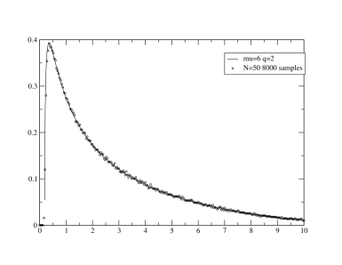
Figure 1: Comparison between the Wishart Student distribution for $Q=2$ and $\mu=6$, solution of the previous equations, and the numerical result obtained for $N=50$ and 8000 samples.

We should however point out that the Pearson estimator is not, in the case of Student variables, the maximum likelihood estimator of $\bf C$. The formula for this estimator was worked out in book and is given instead by the solution of:

$$E^{*}_{ij}=\frac{N+\mu}{T}\sum_{t}\frac{r_{i}^{t}r_{j}^{t}}{\mu+\sum_{mn}r_{m}^{t}(E^{*-1})_{mn}r_{n}^{t}}$$ (12)

This reproduces the usual Pearson estimate when $\mu\to\infty$ at fixed $N$. We are interested in the other limit $N,T\to\infty$ at fixed $\mu$. In this case $\mu$ can be dropped everywhere. As a consequence, the previous equation simplifies into:

$$E^{*}_{ij}=\frac{1}{T}\sum_{t}\frac{\eta_{i}^{t}\eta_{j}^{t}}{N^{-1}\sum_{mn}\eta_{m}^{t}(E^{*-1})_{mn}\eta_{n}^{t}}$$ (13)

Furthermore, in the large $N,T$ limit at fixed $Q$ the denominator in the RHS is expected to become self-averaging and independent of $t$ at leading order. Since the above equation only fixes $E^{*}$ up to an arbitrary multiplicative constant, we fix the value of the denominator to unity, which we can then verify self consistently. Since the $\eta_{i}^{t}$ are Gaussian random variables with unit variance, the maximum likelihood estimator of $\bf C$ is a Wishart matrix, and the eigenvalue spectrum is again given by the Marčenko-Pastur distribution. In order to check that the denominator is indeed equal to unity, we break $E^{*}$ into two contributions: $E^{*}_{1}+1/(T)\eta_{i}^{t}\eta_{j}^{t}$, where $E^{*}_{1}$ is the part of the Wishart Matrix independent of the $\eta_{i}^{t}$. Expanding the expression for the denominator in powers of $1/(T)\eta_{i}^{t}\eta_{j}^{t}$, one finds at leading order in N:

$$(\mbox{Tr}(E^{*})^{-1})/N\frac{1}{1+\mbox{Tr}(E^{*})^{-1}/(Q)}$$ (14)

where we have used that in the large $N,T$ limit $\mbox{Tr}E^{*}/N\approx\mbox{Tr}E^{*}_{1}/N$ and $\sum_{i}(\eta_{i}^{t})^{2}/N=1$. Recalling that the trace of the inverse of a Gaussian Wishart correlation matrix equals $Q/(Q-1)$ one can straightforwardly verify that the denominator is indeed equal to one. We have tested our result by numerical simulation by solving numerically the self-consistent equation (12) for $N=50,80,150$ and $Q=2.5$. The density of states, averaged over $500$ samples, is compared to the Marčenko-Pastur distribution in Fig. 2. The agreement is excellent, thus confirming our analytical result.

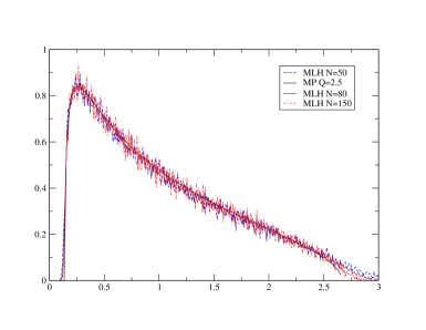
Figure 2: Comparison between the numerical solution of the self-consistent equation (12) for $N=50,80,150$ and $Q=2.5$ (500 samples) and the Marčenko-Pastur distribution. The agreement is excellent. Notice that the blurring of the MP right edge is a finite size effect, as shown by the evolution from $N=50$ to $N=150$.

This result is quite remarkable, especially from the point of view of cleaning noisy correlation matrices. Using the Maximum Likelihood Estimate of $\bf C$ one improves a lot the estimator; it allows to remove completely the effect of the noise due to $\sigma$ fluctuations, in particular to cut the noisy power-law tails of the Wishart-Student distribution.

At this stage, it is interesting to discuss the generality of the above results. First, remark that the DOS could also be computed for an arbitrary correlation true matrix $C_{ij}=\langle\eta_{i}\eta_{j}\rangle$ using free random matrix theory and the so-called S-transform: since in this case ${\bf E}=\sqrt{\bf C}{\bf E}_{WS}\sqrt{\bf C}$, where ${\bf E}_{WS}$ is a Wishart-Student empirical matrix considered above, the eigenvalues of ${\bf E}$ will be the same as those of the product ${\bf C}{\bf E}_{WS}$. The spectrum of $\bf E$ can be computed from the S-tranform of both $\bf C$ and ${\bf E}_{WS}$, extending the classical result for Wishart matrices. Furthermore, our derivation of Eqs. (7,8) does not require Gaussian $\eta_{i}$s but only that $\sum_{i}(\eta_{i}^{t})^{2}/N=1$ for large $N$. Finally, although we focused on a particular shape $P(\sigma)$, Eqs. (7,8) generalizes straightforwardly to any $P(\sigma)$ with not too heavy tails, for example a log-normal distribution.

II.2 Applications to financial data

In the following we compare the Wishart-Student distribution to empirical data. We have considered the daily returns of 450 stocks of SP-500 from 2003 to 2007 and computed the empirical (Pearson) correlation matrices ${\bf E}$ for $Q=2.5$. The resulting average density of states is compared to the Marčenko-Pastur DOS and the Wishart-Student DOS for $\mu=4$ and $\mu=5$. Note that we renormalized the empirical DOS by $1-\sum_{k}^{K_{m}}\lambda_{k}/N$ where $k$ runs over the indexes of the largest $K_{m}$ eigenvalues. As discussed in the introduction, this is done in order to subtract a clearly non random contribution. Although the first few eigenvalues are certainly non-random the precise choice of $K_{m}$ is a subtle matter. Different analysis suggest that $K_{m}\approx 10$ prl . In the following we have chosen to determine $K_{m}$ directly from the Wishart-Student DOS: we determine the values of $\lambda_{0.5},\lambda_{0.9}$ such that the probability that all sampled eigenvalues are less than these values is either 0.5 or 0.9 (of course assuming that the underlying distribution is Student). All eigenvalues that are larger than these cut-offs are assumed to be meaningful. $\lambda_{0.5},\lambda_{0.9}$ depend on $\mu$; furthermore the determination of $K_{m}$ can be altered by other effects not taken into account in our simple model. Therefore we have verified that our results are stable when $K_{m}$ is between $2$ and $10$. In Fig. 3 and 4 we show the comparison between the analytical results, Student and Gaussian Wishart, and the empirical data. We have used 20 samples corresponding to a sliding average with step of $15$ days. The two figures correspond respectively to the $\mu=3.85$ and $\mu=5$ case. In the first case we renormalized the empirical data considering the first or the first two eigenvalue as meaningful. In the second case we considered the first three or the first five as meaningful.

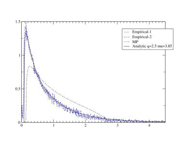
Figure 3: Comparison between the analytical results, Student (for $\mu=3.85$) and Gaussian Wishart, and the empirical data.

The agreement with the Wishart-Student DOS is surprisingly good. The optimal value of $\mu$ appears to be close to $\mu=3.85$ in agreement with the value of $\mu$ obtained from the marginal distribution of daily returns ($\mu\approx 3.85$, see book ). As stressed above these results are not affected much as as long as $K_{m}$ is between $2$ and $10$.

In order to test directly the hypothesis that the returns are multivariate Student variables, we have repeated the same analysis with daily returns scaled by a proxy of the instantaneous volatility, namely:

$$\eta_{i}^{t}=\frac{r_{i}^{t}/\sigma_{i}^{t}}{\sqrt{N^{-1}\sum_{j=1}^{N}(r_{j}^{t}/\sigma_{j}^{t})^{2}}}$$ (15)

and studied the eigenvalue spectrum of ${\widehat{E}}_{ij}=1/T\sum_{t}\eta_{i}^{t}\eta_{j}^{t}$, again subtracting the top eigenvalues. Note that we have normalized each return by $\sigma_{i}^{t}=\sum_{t^{\prime}\neq t}(r_{i}^{t})^{2}/T$ as discussed in book .

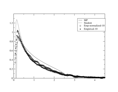
Figure 5: Comparison between the standard DOS of Wishart correlation matrices obtained from empirical data (Empirical-10) and the one obtained renormalizing the returns by a proxy of the daily volatility (Emp-normalized-10). Both are rescaled using $K_{m}=10$ ($Q=2.5$). MP and Student are the analytical Marčenko-Pastur and Student ($\mu=4$) results.

In theory, the resulting spectrum should now be well fitted by the Marčenko-Pastur distribution. As shown in Fig. 5, the spectrum of $\bf{\widehat{E}}$ indeed moves closer to the Marčenko-Pastur result but is still distinctly different. However, the rescaled returns $\eta_{i}^{t}$ are still found have fat-tails; a possible explanation is that the volatility of a given stock fluctuates not only through a common (market) factor $\sigma_{t}$ but also through common sectorial volatilities, which could explain the deviation from Marčenko-Pastur. Another possibility is of course that there are still non-trivial eigenvectors within the “noise blob”. We leave the detailed study of this question for further studies.

III Kullback-Leibler entropy

The Kullback-Leibler (KL) entropy allows one to measure the distance between two probability distributions and is defined in the following way KL :

$$S(2|1)=\int dxP_{1}(x)\log\left(\frac{P_{1}(x)}{P_{2}(x)}\right)$$ (16)

It is easy to show that this entropy is semi-positive definite using that $S_{21}=-\langle\log P_{2}/P_{1}\rangle_{P_{1}}\geq-\log\langle P_{2}/P_{1}\rangle_{P_{1}}=-\log\langle 1\rangle_{P_{2}}=0$. Furthermore its minimum is reached for $P_{1}=P_{2}$. As a consequence it is a possible measure how much the distribution $P_{2}$ differs from $P_{1}$. Note however that it is an asymmetric measure: $S(1|2)\neq S(2|1)$.

Tumminello et al. TLM computed the KL entropy for two multivariate Gaussian distributions with correlation matrices ${\bf C}_{1,2}$ and found:

$$S({\bf C}_{2};{\bf C}_{1})=-\frac{1}{2}\left[\mbox{Tr}\log{\bf C}_{2}^{-1}{\bf C}_{1}+\mbox{Tr}({\bf C}_{2}^{-1}{\bf C}_{1})-\mbox{Tr}{\mathbf{1}}\right]$$ (17)

From this expression, they established that for $N$-multivariate Gaussian variables (stock returns) with true correlation matrix ${\bf C}$, the following holds:

• The average of $S({\bf E};{\bf C})$ is independent of ${\bf C}$ for all $N$ where ${\bf E}$ is the Pearson estimator of ${\bf C}$ on a $T$ long time series: $\langle S({\bf E};{\bf C})\rangle=Z(N,T)$

• The average of $S({\bf E}_{1};{\bf E}_{2})$ is also independent of the true correlation ${\bf C}$, where ${\bf E}_{1},{\bf E}_{2}$ are the empirical correlations corresponding to two independent realisations of the multivariate process described by $\bf C$: $\langle S({\bf E_{1}};{\bf E_{2}})\rangle=Z^{\prime}(N,T)$

This is a very interesting remark because in cases where the a priori distribution is indeed Gaussian one can judge the relative performance of different cleaning procedures of $\bf E$ without knowing the true correlation matrix $\bf C$, by computing $S({\bf E};{\bf E}_{cl})$ where ${\bf E}_{cl}$ is the cleaned empirical correlation matrix. The above two values $Z,Z^{\prime}$ provide interesting benchmark values for $S$. The best one can do is to recover the true correlation matrix: ${\bf E}_{cl}={\bf C}$, so $S({\bf E};{\bf E}_{cl})<Z$ means that some noise remains in the cleaned matrix, while $S({\bf E};{\bf E}_{cl})>Z$ means that the cleaning is too violent and introduces some distortion. On the other hand, the most trivial cleaning procedure is doing nothing: ${\bf E}_{cl}={\bf E}$. Therefore, considering two independent realizations, a good cleaning procedure should be such that $S({\bf E}_{1};{\bf E}_{2,cl})\leq Z^{\prime}$. Furthermore, $Z^{\prime}$ is also interesting to estimate the reproducibility of the filtering procedure by comparing it to $S({\bf E}_{1,cl};{\bf E}_{2,cl})$, see the discussion in TLM . We also remark also that the value of the KL entropies cited above (divided by $N$) is self-averaging in the limit of a very large number of stocks $N$.

As discussed above, the distribution of stock returns is not Gaussian but rather multivariate Student with an exponent $\mu\approx 4-5$. [Note that the marginal distribution of single stock returns is then also found to be a Student-t distribution]. In order to apply the above ideas to real data, we need to extend the results of Tumminello et al. TLM to multivariate elliptic distributions, parameterized by an arbitrary distribution $P(s)$ of the inverse variance. As explained above, the Gaussian case corresponds to $P(s)=\delta(s-\overline{\mu})$ and the Student case corresponds to $P(s)=s^{\mu/2-1}e^{-s}/\Gamma(\mu/2)$.

III.1 Kullback-Leibler entropy for elliptic laws

In order to compute $S(2|1)$ for generic elliptic laws one has to compute:

$$S_{12}=\int d{\bf x}P_{1}({\bf x})\log\left(P_{2}({\bf x})\right),$$ (18)

where ${\bf x}$ is an $N$-dimensional vector. The Kullback Leibler entropy will then be obtained as $S_{11}-S_{12}$. Therefore all constant terms, i.e. independent of the correlation matrix ${\bf C}$, cancel between the two contributions.

A general expression for $S_{12}$ can be worked out using replicas:

$$S_{12}=\lim_{n\rightarrow 0}\partial_{n}\int dx_{1}...dx_{N}\,P_{1}(P_{2})^{n}.$$ (19)

For any positive integer $n$ one can plug into the above equation the general expression of multivariate elliptic laws and find the following expression for $S_{12}$:

$$\lim_{n\rightarrow 0}\partial_{n}\int dx_{1}...dx_{N}\,dsds_{1}...ds_{n}P(s)s^{N/2}\prod_{a=1}^{n}P(s_{a})s_{a}^{N/2}\frac{\exp\left(-\frac{1}{2}\sum_{i,j}x_{i}x_{j}[s{\bf C}_{1}^{-1}+\sum_{a}s_{a}{\bf C}_{2}^{-1}]_{ij}\right)}{\sqrt{2\pi}^{N(n+1)}\sqrt{\det{\bf C}_{1}\det({\bf C}_{2})^{n}}}$$ (20)

One can now integrate out the $x$ variables and get:

$$S_{12}=\lim_{n\rightarrow 0}\partial_{n}\int dsds_{1}...ds_{n}P(s)\prod_{a=1}^{n}P(s_{a})s_{a}^{M/2}\left(\frac{1}{\sqrt{2\pi}^{N}\sqrt{\det({\bf C}_{2})}}\right)^{n}\frac{1}{\sqrt{\det[{\mathbf{1}}+{\bf C}_{2}^{-1}{\bf C}_{1}\sum_{a}s_{a}/s]}}$$ (21)

Introducing the following identity in the previous expression:

$$\int dy\delta\left(y-\sum_{a}s_{a}\right)=\int dyd\hat{y}\exp(-iy\hat{y}+i\hat{y}\sum_{a}s_{a}),$$ (22)

one can finally make the analytic continuation to real $n$:

$$S_{12}=\lim_{n\rightarrow 0}\partial_{n}\int dsdyd\hat{y}P(s)\left(\frac{\int dsP(s)s^{N/2}e^{is\hat{y}}}{\sqrt{2\pi}^{N}\sqrt{\det({\bf C}_{2})}}\right)^{n}\frac{e^{-iy\hat{y}}}{\sqrt{\det[{\mathbf{1}}+{\bf C}_{2}^{-1}{\bf C}_{1}y/s]}}$$ (23)

It is now possible to differentiate with respect to $n$, take the limit $n\to 0$ and get the general expression:

$$S_{12}=-\frac{1}{2}\mbox{Tr}\log{\bf C}_{2}+\int dsdyd\hat{y}P(s)\log\left(\frac{\int dsP(s)s^{N/2}e^{is\hat{y}}}{\sqrt{2\pi}^{N}\sqrt{\det({\bf C}_{2})}}\right)\frac{e^{-iy\hat{y}}}{\sqrt{\det[{\mathbf{1}}+{\bf C}_{2}^{-1}{\bf C}_{1}y/s]}}+K$$ (24)

where $K$ is a constant independent of the ${\bf C}$s. The final expression for the Kullback-Leibler entropy is therefore:

$$S(2|1) = -\frac{1}{2}\mbox{Tr}\log[{\bf C}_{2}^{-1}{\bf C}_{1}]-\int dsdyd\hat{y}P(s)\log\left(\int dsP(s)s^{N/2}e^{is\hat{y}}\right)\frac{e^{-iy\hat{y}}}{\sqrt{\det[{\mathbf{1}}+{\bf C}_{2}^{-1}{\bf C}_{1}y/s]}}+$$ (25)

$$\int dsdyd\hat{y}P(s)\log\left(\int dsP(s)s^{N/2}e^{is\hat{y}}\right)\frac{e^{-iy\hat{y}}}{(1+y/s)^{N/2}}$$

An important remark that will be very useful below is that this expression can be written in general as $S(2|1)=\mbox{Tr}f({\bf C}_{2}^{-1}{\bf C}_{1})$, where $f$ is a function that depends on $P(s)$. In the following we will apply the general expression above to the Gaussian case, to check its validity, and to the Student case.

III.1.1 Gaussian distribution

Let us focus on the multivariate case when $P(s)=\delta(s-\overline{\mu})$. In this case the second term in the general expression above simplifies considerably. Up to a constant term that cancels out between the second and the third term and after rescaling $y,\hat{y}\rightarrow\hat{y}\overline{\mu},y/\overline{\mu}$ we find:

$$-i\int d\hat{y}dy\frac{\hat{y}e^{-iy\hat{y}}}{\sqrt{\det[{\mathbf{1}}+{\bf C}_{2}^{-1}{\bf C}_{1}y]}}$$ (26)

Integrating over $\hat{y}$ one gets:

$$\int dy\delta^{\prime}(y)\frac{1}{\sqrt{\det[{\mathbf{1}}+{\bf C}_{2}^{-1}{\bf C}_{1}y]}}=\frac{1}{2}\partial_{y}\left.\mbox{Tr}\frac{{\bf C}_{2}^{-1}{\bf C}_{1}}{{\mathbf{1}}+{\bf C}_{2}^{-1}{\bf C}_{1}y}\right|_{y=0}=\frac{1}{2}\mbox{Tr}[{\bf C}_{2}^{-1}{\bf C}_{1}]$$ (27)

Repeating the same procedure for the third term, we finally recover the expression derived in TLM :

$$S(2|1)=\frac{1}{2}\left[-\mbox{Tr}\log{\bf C}_{2}^{-1}{\bf C}_{1}+\mbox{Tr}({\bf C}_{2}^{-1}{\bf C}_{1})-\mbox{Tr}{\mathbf{1}}\right],$$ (28)

which can indeed be obtained in a much simpler way.

III.1.2 Student distribution

In order to proceed we have first to compute:

$$\int dsP(s)s^{N}e^{i\hat{y}s}$$ (29)

which in the case of a Student distribution $P(s)=s^{\mu/2-1}e^{-s}/\Gamma(\mu/2)$ reads:

$$\frac{\Gamma(N+\mu/2)}{\Gamma(\mu/2)}(1-i\hat{y})^{-N-\mu/2}$$ (30)

We will use this identity to simplify the second term of (25) finding:

$$\frac{N+\mu}{2}\int dsdyd\hat{y}P(s)\log\left(1-i\hat{y}\right)\frac{e^{-iy\hat{y}}}{\sqrt{\det[{\mathbf{1}}+{\bf C}_{2}^{-1}{\bf C}_{1}y/s]}}+K^{\prime}$$ (31)

In order to be able to integrate over $\hat{y}$ we apply the identity $\log z=\int_{0}^{\infty}(e^{-t}-e^{-zt})/t$ to $z=1-i\hat{y}$. Hence, we obtain:

$$\frac{N+\mu}{2}\int dsdtP(s)\left(\frac{\exp(-t)}{t}-\frac{\exp(-t)}{t\sqrt{\det[{\mathbf{1}}+{\bf C}_{2}^{-1}{\bf C}_{1}t/s]}}\right)$$ (32)

The double integral is dominated by small values of $t/s$ such that the leading contribution can be obtained expanding to the first order in $t/s$. This can be readily checked when ${\bf C}_{2}^{-1}{\bf C}_{1}=\mathbf{1}$. Thus, in the large $N$ limit, one finds:

$$\frac{N+\mu}{2}\int dsdtP(s)\left(\frac{\exp(-t)-\exp(-t-t\mbox{Tr}{\bf C}_{2}^{-1}{\bf C}_{1}/(2s))}{t}\right)$$ (33)

Using again the integral expression of the logarithm we find that the second term of (25) reads:

$$\frac{N+\mu}{2}\int dsP(s)\log\left(1+\mbox{Tr}{\bf C}_{2}^{-1}{\bf C}_{1}/2s\right)$$ (34)

Putting all pieces together we find finally the expression for the Kullback-Leibler entropy for multivariate student distributions:

$$S(2|1)=-\frac{1}{2}\mbox{Tr}\log[{\bf C}_{2}^{-1}{\bf C}_{1}]+\frac{N+\mu}{2}\int dsP(s)\log\left(\frac{1+\mbox{Tr}{\bf C}_{2}^{-1}{\bf C}_{1}/2s}{1+N/2s}\right)$$ (35)

This expression allows one to recover the Gaussian case above in the limit $\mu/N\rightarrow\infty$, where $s\sim\mu/2\gg N$. As a consequence one can expand the logarithm and find the previous expression for Gaussian distribution. The case of interest here is instead $\mu/N\ll 1$. In this case the previous expression simplifies into:

$$S(2|1)=-\frac{1}{2}\mbox{Tr}\log[{\bf C}_{2}^{-1}{\bf C}_{1}]+\frac{N}{2}\log\left(\mbox{Tr}{\bf C}_{2}^{-1}{\bf C}_{1}/N\right)$$ (36)

One can change continuously from the Gaussian case to the Student case by tuning the parameter $x=N/\mu$ in the large $N,\mu$ limit. Gaussian and Student correspond respectively to $x=0,\infty$. Note that the final expression is independent of $\mu$ in the $x=\infty$ case, at least its leading contribution in $N$ which is what we are interested in.

III.2 Applications

Following TLM we shall now compute $Z/N$ and $Z^{\prime}/N$, i.e. $S_{KL}({\bf C}_{1},{\bf C}_{2})$ when ${\bf C}_{1}={\bf E}_{1}$ is the empirical correlation matrix generated from the a priori correlation matrix ${\bf C}$ and ${\bf C}_{2}$ is either equal to ${\bf C}$ or is another independent empirical correlation matrix ${\bf E}_{2}$. The crucial results of TLM is that these expectation values are independent of the true correlation matrix ${\bf C}$. This is in fact true in the case of a general multivariate elliptic distribution since the final expression can be written as $\mbox{Tr}f({\bf C}_{2}^{-1}{\bf C}_{1})$. A generic empirical correlation matrix ${\bf E}$ can indeed be written as: ${\bf E}=\sqrt{{\bf C}}{\bf E}_{0}\sqrt{{\bf C}}$ where ${\bf E}_{0}$ is a Wishart correlation matrix of independent random variables. As a consequence the contribution of ${\bf C}$ cancels out from traces of powers of ${\bf E}_{2}^{-1}{\bf C}_{1}$ and one gets, for example:

$$S(2|1)=\mbox{Tr}f({\bf E}_{1}^{-1}{\bf C})=\mbox{Tr}f({\bf E}_{0}^{-1})$$ (37)

i.e. as found in TLM , the Kullback-Leibler entropy does not depend on the a priori correlation matrix ${\bf C}$. However, its value depends on $P(s)$. In order to compare to real data we will compute explicitely these entropies for Gaussian and Student distributions. Both are expected to be self-averaging quantities in the large $N$ limit.

III.2.1 Gaussian

Calling $\rho_{MP}(\lambda)$ the Marčenko-Pastur density of states of the empirical correlation matrices (with ${\bf C}={\bf 1}$) we find, from the general expression above:

$$\frac{S({\bf E};{\bf C})}{N}=\frac{1}{2}\int d\lambda\rho(\lambda)[-\log\lambda+1-\lambda]$$ (38)

In order to compute $S({\bf E}_{1};{\bf E}_{2})$ one has to calculate $\mbox{Tr}{\bf E}_{1}^{-1}{\bf E}_{2}/N$. This can be performed noticing that the distribution law for these matrices is invariant under arbitrary independent rotations. Therefore we find

$$\langle\mbox{Tr}{\bf E}_{1}^{-1}{\bf E}_{2}/N\rangle=\frac{1}{N}\langle\sum_{a,b}\frac{1}{\lambda_{a}}|\langle a|b\rangle|^{2}\lambda_{b}\rangle=\frac{1}{N^{2}}\langle\sum_{a,b}\frac{1}{\lambda_{a}}\lambda_{b}\rangle=\int d\lambda\rho_{MP}(\lambda)\lambda\int d\lambda\rho_{MP}(\lambda)\lambda^{-1}$$ (39)

Hence, the final result is:

$$\frac{S({\bf E}_{1};{\bf E}_{2})}{N}=-\frac{1}{2}+\frac{1}{2}\int d\lambda\rho_{MP}(\lambda)\lambda\,\int d\lambda\rho_{MP}(\lambda)\frac{1}{\lambda}$$ (40)

It can be shown that these expressions coincide with the ones of TLM in the large $N$ limit.

III.2.2 Student

Calling now $\rho_{S}(\lambda)$ the density of states of the Wishart-Student matrices computed in section II above, we find:

$$\frac{S({\bf E};{\bf C})}{N}=-\frac{1}{2}\int d\lambda\rho_{S}(\lambda)\log\lambda+\frac{1}{2}\log\left(\int d\lambda\rho_{S}(\lambda)\lambda\right)$$ (41)

Applying the same argument used in the Gaussian case, one also finds:

$$\frac{S({\bf E}_{1};{\bf E}_{2})}{N}=\frac{1}{2}\log\left(\int d\lambda\rho_{S}(\lambda)\lambda\right)+\frac{1}{2}\log\left(\int d\lambda\rho_{S}(\lambda)/\lambda\right)$$ (42)

The numerical values of these entropies, computed for different $Q=T/N$ and $\mu$’s, are given in the Tables below.

$\mu=3$	$Q=1.5$	$Q=2$	$Q=3$	$Q=5$
$Z/N$	0.645126	0.527893	0.409243	0.303255
$Z^{\prime}/N$	0.990942	0.730459	0.519955	0.361961

$\mu=4$	$Q=1.5$	$Q=2$	$Q=3$	$Q=5$
$Z/N$	0.445103	0.336914	0.233323	0.149822
$Z^{\prime}/N$	0.814573	0.568792	0.376484	0.23867

$\mu=5$	$Q=1.5$	$Q=2$	$Q=3$	$Q=5$
$Z/N$	0.361844	0.263336	0.172947	0.10532
$Z^{\prime}/N$	0.739387	0.502362	0.320584	0.193947

A comparison of these values to financial data, along the same line as TLM , is left for a future work. Note that since the Maximum Likelihood Estimate of the a priori correlation matrix is a Wishart-Gaussian matrix in the large $N$ limit (see section II), the values of $Z,Z^{\prime}$ found by TLM in the case of Wishart-Gaussian matrices turn out to be correct for the Maximum Likelihood Estimate of Student correlation matrices, as very recently found numerically by Tumminello et al. TLM2 .

IV Conclusion

In this work, we have studied in some details a new ensemble of random correlation matrices related to multivariate Student (or more generally elliptic) random variables. We have found the exact density of states for the Pearson estimate of the correlation matrix for uncorrelated variables, that generalizes the Marčenko-Pastur result. It would be interesting to know whether the joint distribution of eigenvalues can also be computed exactly in this case. We have shown that for the Maximum Likelihood estimator, the density of states is still exactly given by the Marčenko-Pastur distribution.

The comparison between the theoretical density of states in the Student case and empirical financial data is surprisingly good, in any case much better than the Marčenko-Pastur result. However, we are still able to detect significant systematic deviations, which suggest the need of a richer, non-elliptic model for the joint distribution of returns, or the presence of information carrying, low eigenvalues of the correlation matrix (or both).

Finally, we have computed explicitely the Kullback-Leibler entropies of empirical Student matrices, which are found to be independent of the true correlation matrix, as in the Gaussian case. Using our result on the density of states, we give the exact numerical value of the Kullback-Leibler entropies in various cases of interest.

We thank Fabrizio Lillo for very useful discussions and for sending ref. TLM2 prior to publications, and the organizers of the second Cracow meeting on Random Matrices for providing us with the opportunity to put this work together.

References

- (1) V. A. Marčenko and L. A. Pastur, Math. USSR-Sb, 1, 457-483 (1967)
- (2) J. Baik, G. Ben Arous, S. Péché, Ann. Probab. 33 1643 (2005)
- (3) G. Biroli, J.-P. Bouchaud, M. Potters, Europhys. Lett. 78 10001 (2007).
- (4) P. Vivo, S. N. Majumdar, O. Bohigas, J. Phys. A: Math. Theor. 40 4317 (2007).
- (5) L. Laloux, P. Cizeau, J.-P. Bouchaud and M. Potters, Phys. Rev. Lett. 83, 1467 (1999); L. Laloux, P. Cizeau, J.-P. Bouchaud and M. Potters, Risk 12, No. 3, 69 (1999).
- (6) V. Plerou, P. Gopikrishnan, B. Rosenow, L. N. Amaral, H. E. Stanley, Phys. Rev. Lett. 83, 1471 (1999).
- (7) L. Laloux, P. Cizeau, J.-P. Bouchaud and M. Potters, Int. J. Theor. Appl. Finance 3, 391 (2000).
- (8) M. Potters, J.-P. Bouchaud and L. Laloux, Acta Physica Polonica B, 36 2767 (2005)
- (9) J.-P. Bouchaud and M. Potters, Theory of Financial Risk and Derivative Pricing (Cambridge University Press, 2003).
- (10) Y. Malevergne, D. Sornette; Extreme Financial Risks: From Dependence to Risk Management Springer Verlag (2006).
- (11) J.-F. Muzy, J. Delour, E. Bacry, Eur. Phys. J. B 17, 537-548 (2000).
- (12) for a review, see, e.g.: A. Tulino, S. Verdù, Random Matrix Theory and Wireless Communications, Foundations and Trends in Communication and Information Theory, 1, 1-182 (2004).
- (13) Z. Burda, A. Goerlich, B. Waclaw, Phys. Rev. E 74, 041129 (2006)
- (14) A. C. Bertuola, O. Bohigas, M. P. Pato, Phys. Rev. E, 70, 065102 (2004)
- (15) S. Kullback and R.A. Leibler, Ann. Math. Statist., 22, 79-86 (1951).
- (16) M. Tumminello, F. Lillo and R. N. Mantegna, Phys. Rev. E 76, 031123 (2007)
- (17) M. Tumminello, F. Lillo and R. N. Mantegna, Shrinkage and spectral filtering of correlation matrices: a comparison via the Kullback-Leibler distance, this volume and arXiv:0710.0576.